Dynamics and Control of Fluidized Catalytic Crackers. 3.Designing the Control System: Choice of Manipulated andMeasured Variables for Partial Control
Arnon Arbel, Irven H. Rinard, and Reuel Shinnar*
Department of Chemical Engineering, City College of New York, 138 St. at Convent Ave.,New York, New York 10031
In this paper is presented an evaluation of different control structures for a fluidized catalyticcracker. A systematic methodology for evaluating such structures was developed which issuitable for complex nonlinear processes in which the number of manipulated variables is smallerthan the number of variables that are part of the specifications. It is shown that the choice ofthe control structure and the variables entering it is far more important than that of themultivariable algorithms to be used. Criteria for the choice of the measured and manipulatedvariables entering the dynamic structure are presented. The role of additional so-called slowvariables in steady state control is discussed and demonstrated by examples. It is shown thatlinear algorithms are sufficient for dynamic control but nonlinear considerations dominate thechoice of the control structure. This paper is one of the first that thoroughly discusses thecompromises and choices a designer faces in designing a control system for a complex nonlinearsystem. Areas in need of further research are outlined.
1. Introduction
This is the third part of a series in which theprinciples of controlling complex chemical reactors andplants are discussed. Such processes have two mainaspects in common:1. In general they are nonlinear, and their models
are seldom known accurately.2. The number of variables that need to be controlled
is much larger than the number of manipulated vari-ables available for the control.In most of the cases the second problem is dealt with
by choosing a primary square control structure that hasseveral functions. It stabilizes the system at a desiredsteady state, it serves to filter out the impact ofdisturbances, and it allows one to change the steadystate by changing the set points of the controllers toavoid both specification and process constraints. Thiswas discussed by Shinnar (1981, 1986) and is the mainfocus of this paper. It will be shown that the choice ofthe proper primary control structure is far more impor-tant than the algorithms used in designing the actualcontrol loops for a given structure. There is a large bodyof literature that deals with the design of the controllersonce the structure is chosen, but there are fewercontributions that deal with the choice of the properelements of the structure itself. It will be shown thatwhile linear design methods are often adequate for thetuning of the controller, nonlinear features of the systemto be controlled are dominant in the choice of the controlstructure and the loops inside it. In fact, the conven-tional approach based on linearized models can bemisleading.The example used to demonstrate our approach is the
control of a fluidized catalytic cracker (FCC). By thiswe hope to achieve yet another goal, that of betterunderstanding the control of the FCC. In the first partof this series Arbel et al. (1995a) described in detail a
new model for the FCC. All the analysis of this seriesis based on this model.Before attempting to design a control strategy for a
nonlinear system like an FCC, the nonlinear featuresof the system must be thoroughly understood. Thisincludes multiple steady states, complex bifurcations,and potential stability problems. How to approach thisproblem in general was demonstrated in the second partof the series (Arbel et al., 1995b) using a typical FCCas an example.The outline of this paper is as follows: In section 2
the general principles of partial control are discussedand the criteria for choosing the control structurepresented. In section 3 the FCC control structureschosen for evaluation are described, and some historicbackground is discussed. In section 4 the differentcontrol structures for the partial combustion mode areevaluated. Section 5 deals with control in completecombustion operating mode. Section 6 is a summaryof the results.
2. Partial Control General Principles
The formulation of partial control was outlined for achemical reactor by Shinnar (1981, 1986). A shortsummary of the pertinent aspects follows.2.1. Definition and Concept. Any nonlinear sys-
tem, such as a chemical reactor, can be described by anonlinear model in the general form:
where X* is a vector of the state variables, U a vectorof manipulated inputs,W a vector of inputs that can bemeasured but not manipulated, and N a vector ofunknown and unmeasured inputs.In general, the state vector may be very large. Some
of the states may not be known, or more often may notbe measurable. Moreover, as the system becomes morecomplex less is known about M*. A simplified modelM can be identified by a combination of identificationand mathematical modeling (Aris, 1978; Denn, 1986;Shinnar, 1978). This model will be in the subspace:
* Author to whom all correspondence should be addressed.E-Mail: [email protected]. Tel: (212) 650-6679. Fax: (212) 650-6686.
where Y is a vector of outputs that are measured andmay contain some of the state variables that can bemeasured. X is a reduced vector of the state variablesthat can be recognized. However, not all of Y and Uare used equally in the control system. Some areintegrated into the dynamic control, some are used toadjust set points, and some are used mainly for datalogging and diagnostic purposes. Y and U are dividedtherefore into two subsets. Yd (Ud) contains the processvariables monitored (manipulated) either continuouslyor with small sampling intervals compared to the overalltime scale of the process. Ys (Us) contains the infre-quently measured (manipulated) process variables.From a formal point of view this division of Y into Ydand Ys could be carried out by technique of singularperturbations used in modeling and control of multi-time-scale systems (Kokotovic et al., 1976; Martinez andDrozdowicz, 1989). However, in many cases (includingthe FCC), the decomposition is obvious.There is, however, another way to divide Y into
subspaces that is important for deriving the controlstrategy. Yp is defined as the set of process variablesdefining the product and process specifications andprocess constraints. The elements of Yp may lie in bothYd and Ys, and its dimension is generally smaller thanY. For chemical reactors Yp is seldom completelycontained in Yd and part of it lies in Ys. Next, Ycd, asubset of Yd, is defined as the set of process variableson which the dynamic control strategy is based. Al-though Yd may be quite large, a subset of much smallerdimensions is normally chosen as the basis for thedynamic control. If integral control is to be used, thecontrol matrix must be square, and its dimensions arelimited by the number of manipulated variables avail-able. The elements of Ycd are not necessarily part ofYp, but usually are.The distinction between partial control and exact
control comes in the definition of the control objectives.The objective for exact control is to keep the controlledvariables at their set points. Partial control in generalis a strategy to develop a sufficiently large subset of Uand use it to maintain Yp within prescribed limits:
To achieve the goal of eq 3, a primary dynamic controlsystem, Gcd, is defined first which uses a small set ofmanipulated variables, Ucd, to keep a small set ofmeasured variables, Ycd, at their set points:
The set points Ysscd for this primary matrix are deter-
mined by a steady state control system, Gs, which alsodetermines the steady state values for the rest of thecontrolled inputs U:
where the superscript ss denotes steady state values.Note that it is very important to use all the informationavailable to determine the steady state values for allthose manipulated inputs that do not enterUcd and theset points for the dynamic control Gcd.This is a good place to point out that the approach
outlined above is of course not the only way to deal withpartial control. Another well-known way is model
predictive control (MPC). In theory, if a good overallnonlinear model is available, it is possible to use it todirectly control all manipulated variables, both slow andfast, to monitor the system in the desired operatingspace (see for example Balchen et al., 1992). In somecases this has been applied quite satisfactorily. AnotherMPC approach is known as dynamic matrix control(DMC) (Cutler and Ramaker, 1980) that uses a linear-ized model obtained by step perturbations. However,all the MPC methods assume that the control structureis given while here the purpose is to show how to choosethis structure. Therefore the approach taken in thispaper is essential to properly understand and operatea MPC controller.The problem of enforcing constraints in excess of the
number of manipulatable variables is mentioned brieflyin the context of quadratic dynamic matrix control(QDMC) by Prett and Garcia (1988). A third approachbearing some similarities to partial control is modularmultivariable control (Meadowcroft et al., 1992). Whileall of these approaches deal with the enforcement ofconstraints, none addresses the problem that must besolved in addition, namely, the stabilization of highlynonlinear systems.2.2. Criteria for the Choice of the Primary
Control Structure. Any design, including that ofcontrol structures, is based on compromises. Beforeembarking on the evaluation of different control struc-tures, some design criteria must be defined. A list ofthe proposed criteria is given in Table 1 where the orderis not any indication of importance. The criteria arevery much tied together, and it is almost impossible todiscuss them separately. However, an attempt is madeto define each one by itself.1. Modelability. While accurate models are seldom
available, in most cases laboratory data are. It isessential to know how the measured variables relate tothe specifications and constraints. While accuratepredictions are not needed as feedback is used, the leastone needs is an idea of what are reasonable set pointsand what are the signs of the gains. Further, the modelsensitivity to the estimate of individual variables variesconsiderably. For example, in an FCC reactor temper-ature is strongly constrained by heat and mass balancesand is much less sensitive to kinetic or hydrodynamicparameters as compared to the afterburn temperaturerise in the reactor’s cyclones or flue gas. Also, laboratoryexperiments are seldom adiabatic; most of the dataavailable on reactions are at isothermal conditions. Asthe measured variables in themselves are not the goal,but serve for set point control, their modelability has astrong impact on their suitability for the primary controlmatrix. It is necessary to be able to obtain informationabout how the desired output variables Yp (specificationand constraints) are related to the set points Ycd.2. Dominance. In a reactor with a complex reaction
network, temperature has a strong impact on therelative and absolute rates of all reactions as differentreactions have different activation energies. Thus,temperature is a dominant variable. It is this featurethat allows one to keep a large set of variables within a
Y ) M(X,U,W,N) (2)
Ypj min < Ypj < Ypj max (3)
Ucd ) Gcd(Ycd,W) (4)
(Ycdss, Uss|Ucd∉U) ) Gs(Y|Ycd∉Y,U|Ucd∉U,W) (5)
Table 1. Criteria for Evaluating Possible PrimaryControl Structures
modelabilitydominancenonlinearities and stabilitytime scales of responses to set point change and disturbancessufficiency
2216 Ind. Eng. Chem. Res., Vol. 35, No. 7, 1996
+ +
limited space by manipulating only a smaller numberof set points. Variables other than reactor temperaturemay have similar properties. In partial control it istherefore necessary to choose dominant variables for theset point variables. This is important both for distur-bance rejection and change of operating conditions (orin other words intentional change of the output vector).3. Nonlinearities and Stability Considerations.
The first nonlinear consideration is multiple steadystates. That is, one input setting may result in two ormore sets of outputs. For a given set of inputs theremight be only a range of set points where there aresteady states or where the steady states are desirable.For a system with multiple steady states, all desirablesteady states are unstable in the following sense. Evenif a choice of set points is stable, a strong perturbationin an uncontrolled input might cause the system to driftto another steady state. Further, if operating conditionschange, that stable steady state might change to beunstable. For both cases it is desirable for the controlstructure to keep the process stable. A second nonlinearconsideration is that multiplicities in the inputs leadto multiplicities in the outputs. That is, one set ofoutputs can be reached by two or more sets of inputs.It is important that the control structure is unique inthe sense that it will not lead to a different operatingpoint by choosing the wrong input settings although theoutput set points is correct. Although some of theoutput multiplicities might not be practical, each casehas to be checked. A third nonlinear feature is thechange of the gain around the operating point. For anycontrol loop to be effective, there must be a finite gainbetween the input and the output. In nonlinear systemsthis gain changes from operating point to operatingpoint and may even change sign. Thus, the operatingpoint must be chosen such that the gain stays reason-able. Since the gains at different operating points maychange their magnitude as well as their sign, theirrelation to modelability is an important considerationin choosing a control structure.4. Time Scale of Responses. While fast response
is an important criterion in the design of the controlloops, it is not the overriding criterion in the choice ofthe structure. Rather, it is one of several, often conflict-ing criteria which the designer must take into account.Very often in the literature there is an emphasis onchoosing a variable that has a fast and smooth response.However, fast response is only useful if the variablechosen is a critical specification of the process or it is adominant variable. For example, an FCC has a largethermal holdup. As a result the regenerator tempera-ture responds very slowly. This is beneficial as thesystem is damped and the thermal inertia protects itby giving the operator more time to take action. Slowresponse is often intentionally introduced by the de-signer and is essential for the controllability of uncertainsystems. On the other hand, a hydrocracker is sensitiveto very small perturbations in inlet temperature, andtherefore fast control of the inlet temperature is es-sential (Silverstein and Shinnar, 1982).5. Sufficiency. A very important criterion in the
design of any control system is to match the capabilityof the control to the desired specifications (of bothprocess and products) and constraints. This criterionis not an independent one but based on the criteria 1-4,nor is it easily definable. Specification are a result ofboth market demand and process capabilities. Processcapabilities are strongly determined by the plant design
as well as by the number and nature of manipulatedvariables. These are determined during the design ofthe plant. Many times plants encounter severe controlproblem due to changed specifications that are incon-sistent with the capabilities of the plant. The minimumrequirement for any complex reactor is that the controlshould be able to keep it stable in the face of reasonableperturbations, but in most cases much more than thisis required. This is a highly neglected area both inresearch and practice. Estimating these capabilitiesand their relation to initial design or needed modifica-tions is a critical area for the design of the controlstructure as well as of the process.Note that all five criteria have both linear and
nonlinear aspects. All but criterion 3 can be definedby using linear examples. In practice the importanceof nonlinear considerations changes from process toprocess. However, when nonlinear considerations areimportant they are more critical in the choice of thecontrol structure and much less so in the tuning andchoice of the control algorithms for control of a specificsteady state.
3. FCC Control Problem
In this section the partial control approach is appliedto the control of the FCC. The first step of theevaluation is to define the reduced model M of eq 2 forthe process. This was done for the FCC in part 1 ofthis series (Arbel et al., 1995a). All the discussion andresults presented are based on that model. Table 2gives a list of input and output variables for the FCC.It is immediately clear that the number of manipulatedvariables available is much smaller than that of outputsto control.The list in Table 2 is in no way exhaustive. Specifica-
tions and design have evolved with time, increasing thenumber of both control and manipulated variables.Feed stocks have continuously changed, as have cata-lyst, due to the need to treat heavier crudes and due tohydrotreating. As the constraints on gasoline specshave changed, so have the demands on the productslate. Environmental constraints on CO, NOx, and SO2emissions were unknown until the late 1960s. Thesepushed forward the use of catalyst additives to controlemissions as well as the move to operate at full COcombustion in the regenerator.
Table 2. List of Variables for FCC
Manipulated Variables
fast slow
air flow rate catalyst propoerties and additivescatalyst flow rate (combustion promoter, etc.)feed temperature feed ratecatalyst cooler feed quality
Specifications
product constraints
octane CO, NOx, SO2 in flue gas,conversion wet gas ratealkylation feed air rate,gasoline yield cat. circulation ratelight cycle oil yield and properties flue gas temperatureC2 riser temperatureisobutene, propylene to propane ratio regenerator temperature
Model State Variablesriser temperature coke on regenerated catalystregenerator temperature coke on spent catalystregenerator wall temperature
Ind. Eng. Chem. Res., Vol. 35, No. 7, 1996 2217
+ +
Using the notation of section 2, it is possible to definethe different vectors for the FCC on the basis of Table2:
The design of the unit has the largest impact oncontrol via the number of manipulated variables avail-able for control. Many old FCC units still have limitedability to vary catalyst circulation rate rapidly and overa wide range (Avidan and Shinnar, 1991; Huq et al.,1994). Feed preheaters were also less common 25 yearsago, but most units are equipped with them now.Catalyst coolers are slowly being introduced.When the optimization of a unit is considered, it is
very important not to limit the control to the primarycontrol structure but to include feed composition andcatalyst management. But, before any optimization isapplied, the primary control structure is crucial forfiltering disturbances and maintaining stability. Thefocus of this paper is on the choice of this structure. Infact, it is limited to an even more specific example. Thatis the case common to many plants where the manipu-lated variables for the primary control structure are airrate and catalyst circulation rate. This eliminates fromthe evaluation a very critical part of designing a primarycontrol structure, namely, the choosing of the manipu-lated variables. This is best if done during the designof the unit itself, because adding manipulated variableslater is usually very expensive. A future paper willdiscuss the more general problem of the impact of thetype and number of manipulated variables available.In industry and in the literature, different combina-
tions of measured variables have been proposed for thisstructure when operating in partial CO combustion andare given in Table 3. For steady state control, it is notimportant how the variables are connected. It is,however, in dynamic control. The conventional pairingsare given in Figure 1. Table 3 and Figure 1 also containone combination [Tris, O2,sg, Fcat, Fair] which is used onlyin complete combustion and is the only one the authorsare aware of being used in that regime that is based onusing Fcat and Fair as the manipulated variables.Historically for this type of reactor, the set [∆T, Tris,
Fair, Fcat] was used first with various definitions of ∆T((Tsg - Trgn(bed)), (Tsg - Tcyclone entrance), etc.). In partialcombustion, ∆T across the cyclones is related to theamount of uncombusted oxygen entering the cyclones.
The ∆T used here (Tsg - Trgn) is slightly more complexbecause it contains some afterburn in the dilute phase(see part 1) but behaves very similarly, and the resultspresented apply to both cases. However, cyclone tem-peratures are very often not uniform, and these resultsdo not apply when the hot (maximum) cyclone temper-ature is used instead of an average cyclone temperature.The impetus for the use of ∆T and Tsg was two-fold.
First was the need to protect the cyclones from excesstemperatures. When there are problems with airdistribution, some cyclones can get hotter than othersand in old designs this could lead to holes in thecyclones. This was solved by using better materials orby injecting steam into the hot cyclones. The secondreason for the use of ∆T and Tsg was the belief that ahigh ∆T is beneficial as it indicates excess oxygen andtherefore a cleaner regenerated catalyst. As can be seenfrom Figure 2, for operation in partial combustion,increasing air rate (shown as air/oil) while Fcat (shownas cat/oil) is fixed decreases ∆T and reduces Crgc. Inclosed loop, when Tris is kept constant by manipulatingFcat, this trend reverses, and now increasing air rateleads to an increase in both ∆T and Crgc, the latter dueto a decrease in Trgn. The use of Tsg instead of ∆T wassuggested for similar reasons, but its behavior is morecomplex because, as was shown in part 2, it hasmultiplicities in the region of interest and therefore can,
Table 3. Possible Combinations of Manipulated andControlled Variables for Primary Control Structures
regimecontrolledvariables
manipulatedvariables
partial CO combustion Tris, TrgnTris, ∆TTris, Tsg Fair, FcatTrgn, ∆T
complete CO Tris, O2,sgcombustion
Ud ) {Fair, Fcat, Tfeed, catalyst cooler duty}
Us ) {catalyst properties (A, z, additives),Ffeed, feed quality and composition}
Yd ) {Tris, Trgn, Tsg, ∆T, O2,sg}
Ys ) {octane, conv., Yg, Ywg, Crgc, etc.}
Yp ) {all product specs, all operating constraints}
Figure 1. Five possible pairings for primary control structures.
Figure 2. ∆T and Crgc vs air/oil: open loop (constant cat/oil ) 6)and closed loop (Tris ) 1000 °F).
2218 Ind. Eng. Chem. Res., Vol. 35, No. 7, 1996
+ +
in closed loop, change the sign of the gain dependingon the operating point.The scheme [Trgn, ∆T, Fair, Fcat] was suggested by
Kurihara (1967) to stabilize the system and was claimedto have advantages for dynamic control. That it foundno widespread use as control of reactor temperature isvery important (Shinnar, 1976). Stability used to be asignificant concern, as units frequently crashed in thesense that they lost the upper steady state and startedto wind down. This normally occurred when a heavierfeed was introduced. It was shown in part 2 thatheavier feeds increase the range of temperatures atwhich the system is open loop stable. Therefore, openloop instability could not have been the cause of thesecrashes. It will be later shown that these were nonlin-ear effects of the choice of the primary control structure.
4. Evaluation of the Control Structures forPartial Control
The next step in the evaluation is to examine thecontrol structure combinations of Table 3 in the lightof the criteria set in section 2. This will be done inreference to the four sets of operating conditions sum-marized in Table 4. As stated in the last section theconcern is with design compromises, as some structuresmay have advantages for some criteria and be inferiorfor others. Because there are strong interactions be-tween the criteria, it is difficult to discuss them com-pletely separately. They will be dealt with as they arisein the discussion.4.1. Input Multiplicities and the Constraint of
Finite Gain. First, let us review some results of part2 from this series (Arbel et al. 1995b) that dealt withmultiple steady states and instabilities. Two points arecrucial for understanding the control needs:(a) Output Multiplicities: For a large range of inputs
FCC has three steady states, one of which is cold.Sufficiently strong perturbations can crash the unit tothat state.(b) Input Multiplicities: No combination of two output
variables defines a unique steady state. One of theinputs (Fcat or Fair) has also to be specified for unique-ness.
The input multiplicities for the case [Trgn, Tris] aregiven in Figure 3. Note that every operating point inpartial combustion has a counterpoint with the sameset points of [Tris, Trgn] but at a much higher air rate,while cat/oil remains almost constant. Such high airrates are not feasible in a real unit subject to operatingconstraints. Thus, the operating regime in partialcombustion has no reachable multiplicities.But even if a structure has input multiplicities in the
practical range of partial combustion, that does notmean that control would be difficult or that there wouldbe stability problems. Morari (1985) has shown thatfor a single loop, input multiplicities are normally nota problem. In most cases the sign of the gain is differentfor the two steady states. In a single loop an integralcontroller cannot stay stable if the sign of the gainchanges. However, in a nonlinear system, it is perfectlypossible, though much more rare, to have input multi-plicities with both states having gains of the same sign.For a 2× 2 matrix this is even more complex; the steadystate can stay stable in special cases when both signsare reversed.One cannot analyze a stability problem solely by
relying on steady state maps such as that in Figure 3.There are, however, several other important constraintsthat one can deduce from such maps. Note in Figure 3that there are both a maximum and a minimum whereTrgn is not controllable with Fair keeping Tris constant.The lower minimum is outside the present operatingregion. This could change if the operation of an FCCwith a temperature sensitive catalyst becomes of inter-est. For present operation the upper maximum isimportant since it is in the operating region for full COcombustion. Also note that there are set point combina-tions which do not correspond to a feasible steady state,a problem discussed in part 2.In part 2, from which Figure 3 is taken, the complete
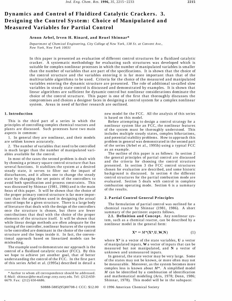
range of permissible air rates was given as the topologyof the steady states was discussed. Figure 4 shows onlythe practical range of air rates for four structures. Alsoshown is the effect of increasing the coking rate, aschanges in the coking tendency of the feed are the mostcommon perturbation in the FCC. Figure 4 clearlyindicates that in full CO combustion, the structure [Trgn,Tris] is not useful, even in the area where the gain isfinite but small. An increase in coking rate wouldincrease Trgn far above the control capability of thestructure. This also refers to the structures [Tris, Tsg]and [Tris, ∆T]. The only solution in full combustion isto use the structure [Tris, O2,sg] whose main purpose is
Table 4. Four Operating Points and Conditions Used inthe Examples
Figure 3. Input multiplicities for [Tris, Trgn]: cross cut at constantTris ) 1000 °F. Tris is kept constant by adjusting cat/oil (some cat/oil values are shown).
Ind. Eng. Chem. Res., Vol. 35, No. 7, 1996 2219
+ +
to keep the unit in the full combustion regime. Thiswill be discussed further.The structure [Tris, ∆T] has properties similar to [Trgn,
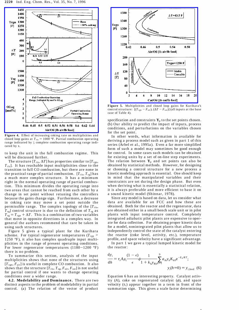
Tris]. It has reachable input multiplicities close to thetransition to full CO combustion, but there are none inthe practical range of partial combustion. [Tris, Tsg] hasa much more complex structure. It has a minimumright in the normal operating range of partial combus-tion. This minimum divides the operating range intotwo areas that cannot be reached from each other by achange in set point without retuning the controllersbecause the gains change sign. Furthermore, a decreasein coking rate may move a set point outside thepermissible range. The complex topology of the [Tris,Tsg] control structure is due to the definition of Tsg asTsg ) Trgn + ∆T. This is a combination of two variablesthat move in opposite directions in a complex way. Ingeneral the authors recommend that care be taken inusing such structures.Figure 5 gives a typical plant for the Kurihara
scheme. For typical regenerator temperatures (Trgn >1250 °F), it also has complex quadruple input multi-plicities in the range of present operating conditions.For lower regenerator temperatures (1180-1200 °F)there is no problem.To summarize this section, analysis of the input
multiplicities shows that none of the structures using[Trgn, Fair] is useful in complete CO combustion. It alsoshows that the structure [Tris, Tsg, Fair, Fcat] is not usefulfor partial control if one wants to change operatingconditions over a wider range.4.2. Modelability and Dominance. There are two
distinct aspects to the problem of modelability in partialcontrol. (a) The relation of the vector of product
specification and constraints Yp to the set points chosen.(b) Our ability to predict the impact of inputs, processconditions, and perturbations on the variables chosenfor the set point.In other words, what information is available for
deriving a process model such as given in part 1 of thisseries (Arbel et al., 1995a). Even a far more simplifiedform of such a model may sometimes be good enoughfor control. In some cases such models can be obtainedfor existing units by a set of on-line step experiments.The relation between Yp and set points can also beobtained by statistical methods. However, for designingor choosing a control structure for a new process akinetic modeling approach is essential. One should keepin mind that the manipulated variables and theirconstraints are set during the design phase. But evenwhen deriving what is essentially a statistical relation,it is always preferable and more efficient to base it ona sound kinetic model (Shinnar, 1978).Since any model is based on data, let us consider what
data are available for an FCC and how these areobtained. Both for the reactor and the regenerator, dataare obtained either in a small bench scale unit or in pilotplants with input temperature control. Completelyintegrated adiabatic pilot plants are expensive to oper-ate for data collection. For obtaining proper kinetic datafor a model, nonintegrated pilot plants that allow us toindependently control the state of the catalyst enteringthe reactor (coke level, activity, etc.), temperatureprofile, and space velocity have a significant advantage.In part 1 we gave a typical lumped kinetic model for
the reactor:
Equation 6 has an interesting property. Catalyst activ-ity (A), coke on regenerated catalyst (φ), and spacevelocity (τr) appear together in a term in front of thesummation sign. This gives a scale factor determining
Figure 4. Effect of increasing coking rate on multiplicities andclosed loop gains at Tris ) 1000 °F. Partial combustion operatingrange indicated by |; complete combustion operating range indi-cated by x.
Figure 5. Multiplicities and closed loop gains for Kurihara’scontrol structure: [(Trgn - Fair), (∆T - Fcat)] (all inputs at the basecase of Table 4).
the advancement along a specific composition trajectory.The direction of trajectory in composition space, whichdetermines final product composition, depends on theterms inside the summation sign. Note that the relativemagnitudes of the reaction rates at any point are solelya function of inlet composition and temperature. As theactivation energies are different for the different rateexpressions in eq 6, the final composition is a strongfunction of the temperature history along the riser. Thedifference between the mixed bottom and the toptemperature in a modern riser can be quite large (30-100 °F). This has a very significant impact on productdistribution. Therefore representing a riser by a stirredtank reactor is insufficient if one wants to properlypredict and correlate product composition.This is an interesting aspect of modelability. It is
often not recognized that for control there is a minimummodel complexity that strongly depends on Yp. Themodel given in part 1 was sufficient 20 years ago but isinsufficiently detailed today since Yp has changed.Today the interest is not only in conversion and gasmake but also in gasoline composition and octane aswell as on the composition of the wet gas. These arestrong functions of the temperature profile. For ourpurposes this is not important. All one would have todo to modify the model appropriately is to derive a moredetailed reaction rate matrix with appropriate numberof lumps having the same form of eq 6. This was notdone here as no nonproprietary data are available, andit is not needed for presenting ideas.Looking further at eq 6 note that at constant feed
conditions and catalyst activity the reactor output isdetermined by four factors:1. The term τrFc(1 - ε)/ε which at constant density
and feed rate is solely a function of Fcat, which, whenused to control Tris, is mainly a function of Trgn and Tris.2. Tris, which is a set point adjustable by control.3. Tmix, which is a function of Tfeed, Fcat, and Trgn.4. Crgc.We note that at constant feed composition, feed rate,
Tfeed, and catalyst activity the reactor outlet compositionis determined by Crgc, Trgn, and Tris, where Trgn and Trishave a stronger impact compared to Crgc. While theriser outputs can never be exactly predicted, changingTris and Trgn independently allows one to significantlymove the individual elements of Yp. This feature iscalled dominance.Thus higher values of either Tris or Tmix will give, at
constant conversion, a higher ratio between wet gas andgasoline, increase the octane of the gasoline, andproduce more C4 olefines. While not all of these are inour model it is an important consideration for modernFCC operation. What is in our model, is the impact ofTris and Tmix on the relative coke make at constantconversion. Therefore, the only way to use laboratoryexperiments to construct a model that predicts theimpact of process conditions on Yp is based on knowingand controlling Trgn and Tris, which is another aspect ofdominance.Let us now look at the regenerator. In the regime of
partial combustion the heat balance is dominated by theCO2/CO ratio, which is determined by the relativemagnitude of the reaction rates of carbon and COcombustion (see part 1). The ratio is, therefore, afunction of Crgc and the ratio of the rate constants. Theactivation energies for carbon and CO combustion aredifferent. The CO2/CO ratio at the catalyst surface (theArthur ratio) is also a function of Trgn. Therefore the
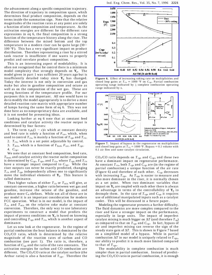
CO2/CO ratio depends on Trgn and Crgc, and these twohave a dominant impact on regenerator performance.At constant Tris, both Trgn and Crgc are (in the regime ofpartial combustion) a unique function of the air rate(Figure 6) and therefore of each other. Crgc decreaseswith increasing Trgn. As Trgn is easier to measure andalso more dominant in the riser, it is normally chosenas a set point. When two dominant variables thatimpact on Yp are coupled with each other there is alwaysan advantage in terms of the controllability of Yp todecouple them. In the case of Trgn and Crgc it requiresuse of additional manipulated inputs such as a catalystcooler. This will be discussed in a future paper.Modeling the regenerator presents a further difficulty.
The fluid dynamics are more complex compared to theriser and have a stronger impact on the performance,especially in large units. The impact of imperfectcatalyst mixing is much bigger on ∆T (and therefore Tsg)as compared to that on Trgn and Crgc. In fact, bypass ofair and imperfect mixing can reverse the sign of thesteady state gain of ∆T. This is shown in Figure 7 basedon a simplified model of a bypass. While in partialcombustion ∆T in our model is uniquely related to Trgn,our ability to predict it is much more limited comparedto that of Trgn.The modelability in complete combustion is much
simpler than in partial combustion. Instead of predict-ing the CO2/CO ratio in partial combustion, it is enough
Figure 6. Effect of increasing coking rate on multiplicities andclosed loop gains at Tris ) 1000 °F on Crgc. Partial combustionoperating range indicated by |; complete combustion operatingrange indicated by x.
Figure 7. Impact of bypass in the regenerator on multiplicitiesand closed loop gains at Tris ) 1000 °F. Bypass ) 0.1 volume with0.1 air flow and same catalyst circulation.
to know that the holdup of air and solids is enough forcomplete combustion. The measurement of excessoxygen in a well-designed regenerator will guaranteecomplete CO combustion and almost complete cokecombustion (Figure 6). As the coke on regeneratedcatalyst is now almost constant and the heat balancedirectly predictable from the coke make the two vari-ables (Crgc and the CO2/CO ratio) that caused thecomplex interactions with the riser are eliminated. Thismakes it much easier to predict unit performance fromlaboratory experiments. However, the ability to controlTrgn by air rate is also lost as was noted in the previoussection (Figure 4). As Trgn is still a dominant variablefor the reactor, this limits the capabilities to control thereactor performance. This will be discussed later.Another aspect of modelability is the permissibility
of a given set of set points. This has several aspectsthat were discussed in part 2 (Arbel et al., 1995b): (a)There may not exist a stable steady state for the setpoints chosen by the operator in which case the unitwill either crash to the cold steady state or move to anew steady state with different Trgn and Tris than thosechosen, with the manipulated variables staying at theirconstraint values. (b) The steady state is permissiblebut the manipulated variables exceed their constraints,a situation that can be corrected by reduction of the feedrate. (c) The unit may become unstable, either due tochange in feed or catalyst properties or by choosing setpoints that have this property. (d) Another constraintis violated which requires change of set points or otheraction.The range of permissible set points was discussed in
Figure 18 of part 2 that gives an example for the limitsfor permissible set points for [Trgn, Tris] for a specificcase. While these limits are not very accurate due tomodel uncertainties and a lack of knowledge of exactcatalyst and feed properties, such plots give guidelinesfor the operator. Similar plots for [∆T, Tris] or [Tsg, Tris]were not given as the model uncertainties are far toolarge to construct such plots from available data.There is yet one more aspect of modelability that
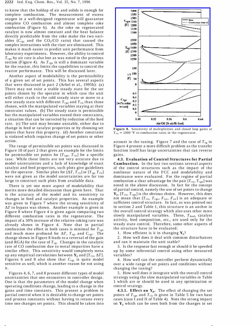
merits more detailed discussion than given here. Thatis the accuracy of the model and its sensitivity tochanges in feed and catalyst properties. An examplewas given in Figure 7 where the strong sensitivity of∆T to bypass was shown. Another example is given inFigure 8 where Figure 4 is given again comparing twodifferent combustion rates in the regenerator. Theimpact of a 30% increase of the relative coking rate wasalready shown in Figure 4. Note that in partialcombustion the effect in both cases is minimal for Trgnand much more profound for ∆T, Tsg, and Crgc. Thechange shown in Figure 8 leads to a reversal of the gain(and RGA) for the case of Tsg. Changes in the catalyticrate of CO combustion due to metal impurities have asimilar effect. This sensitivity would completely messup any empirical correlations between Yp and [Tris, ∆T].Figures 6 and 8 also show that Crgc is quite modelsensitive as well, which is another reason for not usingit.Figures 4, 6, 7, and 8 present different types of model
uncertainties that one encounters in controller design.One is that the parameters of the model change whenoperating conditions change, leading to a change in thegains and time constants. This present a problem inpartial control when it is desirable to change set pointsand process constants without having to retune everytime one changes set points. This should be taken into
account in the tuning. Figure 7 and the case of Tsg inFigure 4 present a more difficult problem as the transferfunction itself has large uncertainties that can reversegains.4.3. Evaluation of Control Structures for Partial
Combustion. In the last two sections several aspectsof the control structures such as the impact of thenonlinear nature of the FCC and modelability anddominance were evaluated. For the regime of partialcombustion a clear advantage for the pair [Tris, Trgn] wasnoted in the above discussion. In fact for the conceptof partial control, namely the use of set points to changeYp, [Tris, Trgn] is the obvious choice. However, this doesnot mean that [Tris, Trgn, Fcat, Fair] is an adequate orsufficient control structure. In fact, as was pointed outin section 2 and Table 1, this structure is an anchor inthe overall control strategy which also uses other moreslowly manipulated variables. These, Tfeed, catalystactivity, feed composition, etc., are used only for thesteady state control. Therefore, some other aspects ofthe structure have to be evaluated:1. How efficient is it in changing Yp?2. How well does it deal with common disturbances
and can it maintain the unit stable?3. Is the response fast enough or should it be speeded
up by some inferential control using other measuredvariables?4. How well can the controller perform dynamically
over a wide range of set points and conditions withoutchanging the tuning?5. How well does it integrate with the overall control
strategy using the slow manipulated variables in Table1 which are or should be used in any optimization orcontrol strategy.4.3.1. Effect on Yp. The effect of changing the set
points of Trgn and Tris is given in Table 5 for two basecases (case I and II of Table 4). Note the strong impacton Yp which can be seen both from the changes in set
Figure 8. Sensitivity of multiplicities and closed loop gains atTris ) 1000 °F to combustion rates in the regenerator.
points and from comparing the two base cases. Asexplained before, the impact is even bigger as Trgn andTris also effect octane and wet gas production. Howeverit has to be admitted here that any of the other controlschemes have a range of set points for which the abilityto control Yp by changing the set points is no less. Thisis due to the fact that in the range of partial combustionfor which a given pair of set points leads to a uniquesteady state, fixing [Tris, ∆T] is equal to fixing [Tris, Trgn].There are two limitations to this statement. The rangeof operating conditions for which this applies is morelimited due to the input multiplicities for [Tris, Tsg] and[Trgn, ∆T] compared to [Trgn, Tris] (Figure 4). But evenmore important, a lot is lost in terms of modelability asall the model predictions for Yp require knowledge ofTrgn and Tris. This would be less of a problem if ∆T orTsg would give a good inferential estimate of Trgn. Thatthis is not so is a special problem of the FCC. As wasshown in section 4.2, ∆T and therefore Tsg are verymodel sensitive and much more sensitive than Trgn tochanges in operating condition. This limits the use of∆T as an inferential estimate for Trgn. As these changesin ∆T and Tsg have little impact on Yp, there is nobenefit in developing a better method to estimate them.One can just as well measure Trgn directly. While ∆Tcan be controlled at fixed operating conditions, it is noteasily integrated into an overall control strategy to takecare of changing operating conditions, feed stocks, andprocess goals.4.3.2. Disturbance Rejection. Table 6 gives the
response of the control at one set point to an increaseof 30% in the coking rate for all four structures. Thisillustrates another point. In the past one aspect of main
concern in FCC control in partial combustion was thefear of a crash. One of the authors (R.S.) has consider-able experience with this issue and has collected evi-dence from other experts. While the detailed data areproprietary, there is one common trend in these occur-rences. They always occurred when a feed with highercoking tendency was introduced either intentionally oraccidentally. This seems strange at first as our analysisshows that more coke would always stabilize the systemboth in open loop and with fixed [Trgn, Tris].Table 6 gives a potential answer to this problem of
crashing. At fixed Trgn and Tris the change in Fair (air/oil) and Fcat (cat/oil) are minimal. One is unlikely torun into a constraint in Fair or Fcat. Conversion and wetgas production are reduced. One could compensate forthe reduction by changing the set points. In the caseof constant ∆T or Tsg, Trgn decreases drastically. Trgnis usually watched by the operator, who would intervenemanually for a strong decrease in Trgn. If the operatorwould increase the air rate, Trgn would further decreaseand crash the unit. It was also observed that Crgcincreased, an effect called “snowballing” (Edwards andKim, 1988). Table 6 shows that this happens in ∆Tcontrol when coking rate increases. This is obvious fromFigure 8 as an increase in Fair at constant Tris alwaysincreases Crgc. The case [Trgn, ∆T], which was intro-duced to stabilize the system, causes a real upset. Thechanges in Fair and Fcat are large and could lead tosaturation of Fair. Further, Tris drops drastically, be-coming uncomfortably close to the lower limit of oper-ability for the riser. This case of [Trgn, ∆T] control is adramatic example of why one cannot use purely linearconsiderations in the choice of a control structure. Also
Table 5. Control Action Needed for Change in Set Points and Resulting Change in Output for the Structure [Tris, Trgn,Fair, Fcat] (Changes Are in Units from Steady State)
case I of Table 4 case II of Table 4
set point change base Tris (+10 °F) Trgn (+10 °F) base Tris (+10 °F) Trgn (+10 °F)
given in Table 6 are the results for the structure [Tris,Crgc]. Note that Trgn increases significantly whichreduces conversion. As Trgn is more dominant and moremodelable than Crgc, Trgn is preferable for disturbancerejection.Table 7 gives similar results for a second case limited
to [Tris, Trgn]. The control is very satisfactory. Somedisturbances can lead to problems while controlling theunit via this structure. If there is a strong decrease incatalyst activity or coking rate, the system can becomeunstable or the settings of Trgn and Tris can becomenonpermissible. An experienced operator will recognizethis, but proper diagnostic methods would here bedesirable but are outside the scope of this paper. Thereis no two-dimensional control structure that can elimi-nate this problem. Increasing Trgn in most casesstabilizes the system.Today this is less of a problem as feed stocks are
heavier and catalysts more active. However, in somecases feed stocks have been hydrotreated and havetherefore lower coking rates. One best take care of suchstability problems by using one of the slow manipulatedvariables, e.g., increasing catalyst activity or adding apromoter to increase the heat supplied by the coke.Also given in Table 7 are some examples to illustrate
the impact of some slow variables. The impact of feedcomposition was already discussed. Also shown is theimpact of increasing catalyst activity as well as reducingfeed temperature after an increase in coking rate. Thefact that Trgn and Tris can be controlled independentlyover a significant range allows, together with controlof feed temperature and catalyst activity, one not onlyto change Yp over a wide range but also to take care ofa wide range of feed stocks albeit with some compro-mises as to conversion and yield.Comparing cases I and II and their perturbations also
shows another interesting aspect of the control. In caseI (higher Trgn and Tris) the conversion increased whilegasoline yield decreased resulting in higher wet gasproduction. This can be beneficial if there is enoughcapacity in the wet gas compressor, gas plant, andalkylation plant. In other cases the opposite may betrue. Increasing catalyst activity further accentuatesthis effect. If a large fraction of the gasoline is cracked,octane increases since the aromatics in the gasolinecrack faster than paraffins. Tables 5, 6, and 7 give agood illustration of what is meant by partial control anddominance.4.3.3. Stability and Time Response. The evalu-
ation of the different control structures in the previous
sections gives a clear advantage to the structure [Tris,Trgn, Fair, Fcat] over the other three structures. It has aclear advantage in modelability and dominance, and itis the only structure for which one can clearly relatethe settings to desired process outputs. It also hasadvantages with regard to multiplicities.For these reasons let us focus on the structure [Tris,
Trgn, Fair, Fcat]. If the system cannot be adequatelystabilized or perturbations that are normally encoun-tered cannot be taken care of, this structure should berejected despite its other advantages. As said before,linear methods can be used as long as the differentsteady states over the expected operating regime inpartial combustion are considered. The problems en-countered in evaluating stabilization and time responseare really not specific to partial control and would occurin any 2 × 2 control problem. However, the results ofthe evaluation are important for evaluating the suf-ficiency of the structure. Including here all four struc-tures would make the paper unnecessarily long espe-cially as it will be shown that the preferred structureis fully adequate.Let us start with the linerized transfer function given
in Table 8 and the controller gain limits given in Table9. Also given in Table 9 are the RGA for differentconfigurations. Note that the RGA’s in Table 9 have anegative diagonal for all the control structures consid-ered for partial combustion.The conventional approach to design (Bristol, 1966;
Shinseky, 1967; Shinseky, 1984; McAvoy, 1983, Hovdand Skogestad, 1994) would give preference to thepairing [(Fair - Tris), (Fcat - Trgn)] along the positivediagonal. However, conventional practice in FCC op-eration has always been [(Fair - Trgn), (Fcat - Tris)] alongthe negative RGA diagonal. This introduces a stabilityproblem. If the loop [Trgn, Fair] fails or is put on manualafter it was tuned with positive gain, the systembecomes unstable. This has been demonstrated in acommercial FCC by Edwards and Kim (1988) and wasdiscussed in part 2. One can however live with that assuch failures are rare, and, fortunately, the system isquite slow to respond, giving the operator ample timeto intervene. In general, in adiabatic reactors a com-petent designer will introduce a slow mode providingsufficient thermal inertia to give the operator time torespond.We are not aware of anybody in industry using the
positive diagonal pairing. While there are many historicreasons for the present scheme the positive diagonalpairing still merits evaluation. It has two disadvan-tages:(1) The first is modelability. It is counter-intuitive.
The central concern of our control is the reactor. Thelaboratory data that underlie our model and controlstrategies are based on decoupled, stand alone labora-tory units in which the reactor is fed a catalyst of fixedtemperature and coke level. Intuitively it would bepreferred to control the regenerator temperature byusing the air flow as a manipulated variable. Thispartially decouples the reactor from the regenerator.The only coupling left is through the coke level onregenerated catalyst. In modern operating conditions(Trgn > 1230 °F) this level is kept low, minimizing theinteractions. On the other hand, controlling the reactorwith air flow involves complex interactions betweenregenerator and reactor that are hard to model ac-curately. Obviously for steady state control this makes
Table 7. Control Action Needed and Changes in Outputsafter a 30% Increase in Coking RatesImpact of UsingSlow Manipulated Variables
no difference, but again it is difficult to think one wayand tune loops another way.(2) The scheme along the positive diagonal does not
allow fast control of Tris. As the holdup of the reactoris low compared to that of the regenerator’s, the decou-pling using the conventional control scheme allowsconceptually fast and easy control of the reactor. Theregenerator provides the slow time scale needed to helpan adiabatic system with multiple steady states andallows the operator to make adjustments without crash-ing. Modern reactors are designed with short residencetime and respond very fast. This was not always so assome other designs had a similar time scale for bothreactor and regenerator.As the emphasis in control is on the reactor in terms
of product properties and conversion, a tight control(1-2 °F) on it is desired. The regenerator dominatesstability considerations. As it responds slowly fastcontrol is not needed nor desired. There is no problemif Trgn changes over a 20 °F range. The fact that it ishard to achieve this goal with the positive diagonalscheme is directly apparent from the dynamic RGAshown in Figure 9. Note that the RGA for the positivediagonal changes to zero at higher frequencies wherethe negative diagonal goes to unity. The RGA does notgive information about the time response of eachseparate loop, but the information in Figure 9 coupledwith the knowledge about the response of the decoupledreactor to Fcat is sufficient to indicate that the chanceof fast control of Tris is better along the negativediagonal.In terms of stability the positive diagonal pair has
no problem. The transfer functions have an overallbehavior that is approximately first order, and theconstraints on control action are dominated by avoid-ance of saturation and oscillatory response. Knowledgeof the RGA is, however, insufficient to show if thecontroller can stabilize an unstable steady state. SuchT
able
8.Transfer
FunctionsfortheCon
trol
Structure
[Tris,Trgn,F
air,Fcat]at
TwoPoints
inPartial
Com
bustion
case
IofTable4:
stablepoint,
Trgn
)1255
°F,T
ris
)1000
°F,T
feed
)670°F
case
IIIofTable4:
unstablepoint,
Trgn
)1230
°F,T
ris
)980°F,T
feed
)400°F
Trgn(s)
Fair(s)(
°Flbair/lbfeed)
1.5(0.0003
+s)(0.005
+s)(0.0084+
s)(0.010
+s)
(0.00029
+s)(0.00085
+s)(0.0047+
s)(0.0093+
s)(0.01+
s)1.3(0.0003
+s)(0.069
+s)(0.012
+s)(0.014
+s)
(-0.00025+
s)(0.00032
+s)(0.0074+
s)(0.0137+
s)(0.015
+s)
Trgn(s)
Fcat(s)(
°Flbcat/lbfeed)
-0.13(0.0003+
s)(0.0095+
s)(0.0047
(i0.0013+
s)(0.00029
+s)(0.00085
+s)(0.00047
+s)(0.0093+
s)(0.01+
s)-0.12(0.0003+
s)(0.0036+
s)(0.0081+
s)(0.0139+
s)(-0.00025+
s)(0.00032
+s)(0.00074
+s)(0.0137+
s)(0.015
+s)
Tris(s)
Fair(s)(
°Flbair/lbfeed)
0.86(0.0003+
s)(0.0055+
s)(0.0084+
s)(0.0099+
s)(0.00029
+s)(0.00085
+s)(0.0047+
s)(0.0093+
s)(0.01+
s)0.86(0.0003+
s)(0.0079+
s)(0.0012+
s)(0.014
+s)
(-0.00025+
s)(0.00032
+s)(0.0074+
s)(0.0137+
s)(0.015
+s)
Tris(s)
Fcat(s)(
°Flbcat/lbfeed)
22(-0.00086+
s)(0.00031
+s)(0.0053+
s)(0.0084+
s)(0.0096+
s)(0.00029
+s)(0.00085
+s)(0.0047+
s)(0.0093+
s)(0.01+
s)18(-0.0019
+s)(0.00031
+s)(0.0075+
s)(0.012
+s)(0.0014+
s)(-0.00025+
s)(0.00032
+s)(0.0074+
s)(0.0137+
s)(0.015
+s)
Table 9. Some Linear Properties of Different ControlStructures
Steady State Gains and RGA for Case I of Table 4
steady state gains RGA
case I
air/oil[°F/(lb
air/lb feed)]
cat/oil[°F/(lb
cat/lb feed)] air/oil cat/oil
Trgn 1716 -74 -1 2Tris 1071 -22 2 -1
Tsg 271 -25 -0.3 1.3Tris 1071 -22 1.3 -0.3
∆T -1445 48 -1.6 2.6Tris 1071 -22 2.6 -1.6
Trgn 1716 -74 -3.6 4.6∆T -1445 48 4.6 -3.6
Proportional Controller Limits, K ) KcGp(0)(Conventional Negative Feedback Control)
case I of Table 4:stable
case III of Table 4:unstable
Trgn/Fcat K > -1.0 K > 1.0Trgn/Fair K > -1.0 K > 1.0Tris/Fcat 0.98 > K > -1.0 5.9 > K > 1.0Tcis/Fair K > -1.0 K > 1.0
With 2% Control Action in Air/Oil and 10% in Cat/Oilthe Maximum Temperature Gain Is
air/oil [°F] cat/oil [°F]
Trgn 34 7.4Tris 21 2.2
Ind. Eng. Chem. Res., Vol. 35, No. 7, 1996 2225
+ +
cases do not arise intentionally but due to changes incoking rate or catalyst activity the gains change. Givenin Figure 10 are stability limits for two steady stateswith different gains, one stable and one linearly un-stable. The stable steady state was chosen for normal-ization. It is asked that the control structure canstabilize well an unexpected change to an unstablestate. The controller along the positive diagonal is aperfectly reasonably controller. The fact that the nega-tive diagonal pairing has in this case decisive advan-tages due to the reasons listed above is very specific tothe FCC. The only conclusion that can be generalizedis that care should be taken in setting up rules. Designis often based on compromises between conflictingcriteria.In Figure 10 the controller constants K were normal-
ized by the steady state gains to reflect conventionalnegative feedback controllers. To judge what K’s arepermissible, one has to look at saturation constraints.Most present FCC’s (but not all) operate very close tothe air constraints and allow no more than 2% fordynamic control. In the past catalyst flow rate wasoften the constraint. At present a 10% leeway incatalyst circulation rate for dynamic control is reason-able. The maximum available steady state compensa-tion in temperature is given in Table 9. The ratiobetween the maximum compensation and the derived
range of temperature to be controlled dynamically givesan estimate as to what K’s are permissible. This is truefor both conventional paring and paring along thepositive diagonal.For integral control based on the positive diagonal
pairing, changing either one or both of the signs of thecontroller’s gains will make the system unstable. Forthe control along the negative diagonal, the sign of thecontroller gains for negative feedback control will bedetermined on which loop is closed first. Shown inFigure 11 are the stability limits for the conventionalparing based on the negative RGA. The system remainsstable with integral control if both signs are reversed.Negative feedback control has here no clear meaning.However, there are two different sign combinations withtotally different properties. Unfortunately, use of theRGA offers no help as it is identical for both choices.For the structure [(Fair - Trgn), (Fcat - Tris)] closing theair loop first is an obvious intuitive choice, based on thesame reasoning used for choosing the negative diagonal.The emphasis is on the reactor so it is better to decoupleit. At constant Trgn it becomes much easier to control,and intuitively it is assumed that increasing catalystflow will increase reactor temperature. It is counter-intuitive that with an uncontrolled regenerator thesteady state gain for the loop [Tris, Fcat] has a negativesign. It is the result of a complex interaction. There-fore, it makes sense to close the air loop first. Thereare other reasons. There is a lot of experience availablewith FCC’s where the only dynamic control is on theregenerator air control. This was common in older unitssuch as Model IV. Units with fast-acting slide valvescame later. It made sense to use the experience fromother units. Since then it was learned that it is hardto control an FCC with fixed air, manipulating only Fcateven if it is desirable to do so to maximize productionrate.There is another intuitive reason why choosing posi-
tive gain for both circuits is preferable. The dynamicRGA indicates that control along the negative diagonalallows complete decoupling at high frequencies. Toutilize these for fast reactor control, it is obvious thatthe sign of the fast initial response of Tris with Fcat(which is positive) must be used. It turns out thatreversing the sign (closing the reactor first) also hasother problems as can be seen from Figure 11. There
Figure 9. Dynamic RGA for the control structure [Tris, Trgn, Fair,Fcat] (all conditions are of case I of Table 4). (s) Main diagonal:[(Trgn, Fair), (Tris, Fcat)]; (- - -) Off diagonal: [(Trgn, Fcat), (Tris, Fair)].
Figure 10. Stability limits change due to transition from stabilityto instability for the control structure [(Trgn, Fcat), (Tris, Fair)] witha P controller starting at case I of Table 4 (stable steady state inpartial combustion).
Figure 11. Stability limits change due to transition from stabilityto instability for the control structure [(Trgn, Fair), (Tris, Fcat)]starting at case I of Table 4 (stable steady state in partialcombustion) with a PI controller: Ki(1 + 0.001/s).
is an obvious problem with the signs normalization insuch figures. However, for this specific example thereis no problem with the symmetries of the gains becauseat this steady state the RGA is -1.0. That means thatclosing one loop first reverses the sign but retains thesame magnitude for the gains. Therefore, the normal-ization of the sign for the negative diagonal pairing isbased on the loop normally closed first. Note fromFigure 11 that the stability limits for negative K (reactorclosed first) are much narrower. There is a simpleexplanation for this. The open loop transfer functionfor Tris/Fcat has a right-hand-side zero, a 180° phase lagat zero frequency. This strongly limits control action.Figure 12 gives the frequency responses of Tris/Fcat withboth loops open and with the Trgn/Fair closed withreasonable integral action. Note that the phase lagdisappears. This is also apparent from Figure 11. IfKrgn is sufficiently large then there are no limits on Kris.Also shown is the open loop response of Trgn/Fair. It isessentially a first-order lag that comes from the thermalinertia of the regenerator.This shows another limitation of the loop with nega-
tive gains (reactor loop closed first). Changes in setpoint or in catalyst or feed properties will change theopen loop gain. Kmax for this loop is the inverse of thenormalized gain, and therefore a controller based onclosing [Tris, Fcat] first could become unstable due tochanges in the gain. While such a controller could inprinciple stabilize an unstable steady state, such astabilization is totally nonrobust due to sensitivity tothe process gain. On the other hand the conventionalcontroller tuning where [Trgn, Fair] is closed first is veryrobust as long as the set points remain permissible. The
stability limits are wide, and the main constraints oncontrol action are oscillatory response and saturation.Properly tuned, these controllers can also stabilize anunstable steady state, but it is preferable to avoid thissituation.Low model sensitivity means that less model infor-
mation is required for control of this loop. Minimummodel information required is a very important consid-eration in the design of control loops for partial controlof complex systems. Regrettably there is no literaturefor designing control algorithms along the negativediagonal. These are highly dependent on model proper-ties and specific goals which cannot easily be general-ized.4.3.4. Time Response. It is important that the loop
finally chosen should have a reasonable time response.It is hard to define a general criterion. The responsehas to be fast enough to stabilize the system againstanticipated perturbations. Perturbations in catalystactivity are slow and do not require fast response.Changes in feed properties can be fast, but in properoperation one tries to protect the unit from suchdisturbances by using a large feed tank as a filter. Nocontrol can adequately operate in an adiabatic reactorif disturbances are not filtered. In some sense the slowtime response of the unit due to thermal inertiaprovided by the catalyst holdup in the regenerator offershere a protection. The cost of this protection is that theregenerator responds slowly.The reactor has very small holdup and in our scheme
it allows very fast response. When the sign is reversedthe reactor control loop has a right-hand zero and istherefore limited due to the inverse response at lowfrequencies. In the positive diagonal, control responseof the reactor loop is slow as it is not decoupled fromthe regenerator holdup.So let us concentrate on the preferred design [Tris,
Trgn, Fcat, Fair] with positive gains. Note from Figures11 and 12 that the main limits on controller gain aredue to saturation of the manipulated variable andoscillating response. The limits on the gains are givenin Table 9. Figure 12 shows that the [Trgn, Fair] loop isapproximately a first-order filter with a time scale ofabout 30 min which limits fast control whereas thereactor loop is approximately a simple gain allowing fastand accurate control. The fact that the regenerator isslow is desirable as it allows the operator to recover frommistakes and deal with changes in operating conditions.Thus the control structure when properly tuned shouldhave adequate time response. A typical set of set pointchanges in Tris and Trgn is given in Figures 13 and 14with two different sets of controller constants. Note thatthe response of the reactor is fast if properly tuned. Itis also shown that reducing the gains of the reactorcontrol gives a smoother and a faster control of Trgn. Thisis a very interesting phenomena that, while theoreticallyknown, has received little attention. If large changesin set points are required, it is preferable to loosen upthe loop that normally is tightly controlled, to make iteasier to move the unit. An interesting parallel problemexists, for example, in economics. Is it possible tostimulate the economy while maintaining tight controlon inflation?Figures 13 and 14 also give the output of the ma-
nipulated variable as a percentage of its value at steadystate. Note that neither variable becomes saturated fora set point change of 5 °F. The time response of theregenerator while slow is adequate. Faster control
Figure 12. Open loop frequency response of: (a) (s) Tris to Fcatopen loop; (b) (- - -) Tris to Fcat when Trgn is controlled by Fair witha PI; (c) (-‚-‚-) Trgn to Fair open loop.
would lead to saturation in most cases, and as saidbefore even then it can only be done if the reactor controlis reduced otherwise the response of Trgn is oscillatory.More complex algorithms based on decoupling couldimprove the operation but are outside the scope of thispaper. For choosing the structure it is sufficient to showthat it can provide adequate control and time response.4.4. Evaluation of the Control Structures for
Complete Combustion. For the operation in completeCO combustion it is a common industrial practice to usecombustion promoters. Even though operation is pos-sible without them, promoters reduce CO emissions and∆T, and thus make the operation smoother. Figure 15shows the effect of the promoter on Trgn and O2,sg atconstant Tris. Also shown in Figure15 are the effects ofhigher activity and higher coking rate. The addition ofpromoter affects the values of Trgn only in partial
combustion. In complete combustion Trgn is not effectby the promoter and still has a flat maximum with Fair.As discussed before, it is therefore not controllable withFair in this region. Using Fcat instead runs a large riskof losing the full combustion because it will increase thedemand for oxygen. The only possibility left using Fairand Fcat is the structure [O2,sg, Tris, Fair, Fcat], and wewill concentrate on its evaluation. For cases where thiscombination proves insufficient, addition of one or moreloops will be considered.The conventional pairing for this structure is [(O2,sg
- Fair), (Tris - Fcat)]. This is also the pairing suggestedby the RGA (see Table 10). The effect of the conven-tional paring is to keep the unit in complete combustionby guaranteeing a minimum of excess oxygen. This isusually maintained below 2% for economic efficiency.It is possible to operate at 0.5% excess oxygen. This
Figure 13. Time response to a step in the set point of Tris. Effectof control of Tris: (1) tight tuning; (2) relaxed tuning (all conditionsare of case I of Table 4).
Figure 14. Time response to a step in the set point of Trgn. Effectof control of Tris: (1) tight tuning; (2) relaxed tuning (all conditionsare of case I of Table 4).
requires more attention as the operation is closer to thestability limit, as can be seen from Figure 15. Whathelps is that in complete combustion Tris increasesalmost linearly with increasing Fcat without any inputmultiplicities because Trgn is almost constant at thisregion.Excess O2 has to be controlled. Otherwise an increase
in coking rate might move the system out of fullcombustion. Aside from keeping the system stable infull combustion, it has no impact on the other variables.
This is illustrated in Table 11 where the effect ofchanging the set points of O2,sg and Tris for case IV ofTable 4 is shown. It does, however, impact on NOx andCO emissions (traces) which are not predicted by ourmodel. Changing the set point of Tris has a strongimpact on conversion and wet gas and also stronglyaffects product properties such as octane and gascomposition.Table 11 also shows the effect of increasing the coking
rate both in open loop and when controlling Tris andO2,sg. When not under control the unit loses completecombustion as discussed above. The main problemwhen under control is the increase in Trgn. Encounteredhere is a problem discussed already in section 4.1. Incomplete combustion the regenerator is much easier tomodel. If the holdup is sufficient and the system ispromoted, the regenerator model is simply a dynamicheat balance. But while modelability is gained, thecapability for partial control is reduced as it is no longerpossible to control Trgn by manipulating Fair. While Trgnis no longer dominant for the regenerator, it is still avery dominant variable with regard to the riser perfor-mance. At a given Tris it controls Fcat and though it Tmix.There are several ways to reduce Trgn. One is to
reduce Tris which is often undesirable because of itsimpact on the product outputs. However, if Trgn in-creases too much, it may be necessary to reduce Tristemporarily as this is the only fast variable that canreduce Trgn. Another way to reduce Trgn is to use anadditional manipulated variable. These can be feedtemperature or a slow manipulated variable such ascatalyst activity or feed composition as discussed insections 2 and 3. These slow variables should be partof any control strategy in complete as well as in partialcombustion. Table 11 shows the impact of using cata-lyst activity and feed temperature to restore conversionor reduce Trgn similar to Table 7. Reducing feedtemperature increases Fcat and therefore conversion andwet gas make. It also significantly increases the airrate. It does not decrease Trgn as also noted in Figure15. Decreasing catalyst activity reduces Trgn with asmaller impact on conversion, which is lower than that
Figure 15. Multiplicities and steady state gains for Trgn and O2,sgvs air/oil at constant Tris ) 1000 °F. Impact of CO combustionpromoter, relative activity, relative coking rate, and feed preheat(all other inputs at base conditions of Table 4; level of promoteras in case IV of Table 4).
Table 10. Transfer Functions, Open Loop Gains, and RGA for the Control Structure [Tris, O2,sg, Fair, Fcat] in CompleteCombustion
Transfer Functions
stable point in complete combustion, case IV of Table 4:Trgn ) 1388 °F, Tris ) 1000 °F, Tfeed ) 670 °F, Xpt ) 5
in the base case. The main variables for control of Trgnare therefore the slow ones such as feed composition andcatalyst activity.While operating in complete combustion has some
advantages such as cheaper investment (no CO boiler),it reduces the overall control capabilities and the abilityto process heavier feed stocks. One option to overcomethis is a catalyst cooler. A catalyst cooler allows one tocontrol Trgn independently which removes all the controldisadvantages of operating in complete combustion.Not only is modelability easier for complete combus-
tion but so are dynamic stabilization and control. Thestability problem in complete combustion is differentthan in partial combustion. Due to the presence ofcombustion promoters, all practical complete combus-tion controller settings with 0.5-2% excess oxygenrepresent stable steady states. Low activity or lowcoking rate could drop Trgn below 1320 °F wherecomplete combustion is hard to achieve without promo-tion. With sufficient promoter it is possible to go evenlower, say to 1270 °F, while staying in complete com-bustion. So the stability problem is one of preventingthe loss of complete combustion because of insufficientair or too low Trgn. Figure 15 shows that lower cokingrate and lower Tfeed require more air, and since mostunits operate close to maximum air capacity, caution ishere advised. A constraint on air rate can always beremoved by reducing the feed rate.The need to keep the unit in full CO combustion has
a interesting implication with respect to stability. Inpartial combustion failure of the loop [Trgn, Fair] meansthat the unit becomes unstable due to the negative RGA.Here the RGA is positive, but this is of no help. If theexcess air is low and the air loop fails, the unit can, aftera perturbation in coking rate, either crash or go topartial combustion. Thus operating close to the airconstraint is not advisable.The transfer functions for the structure [O2,sg, Tris,
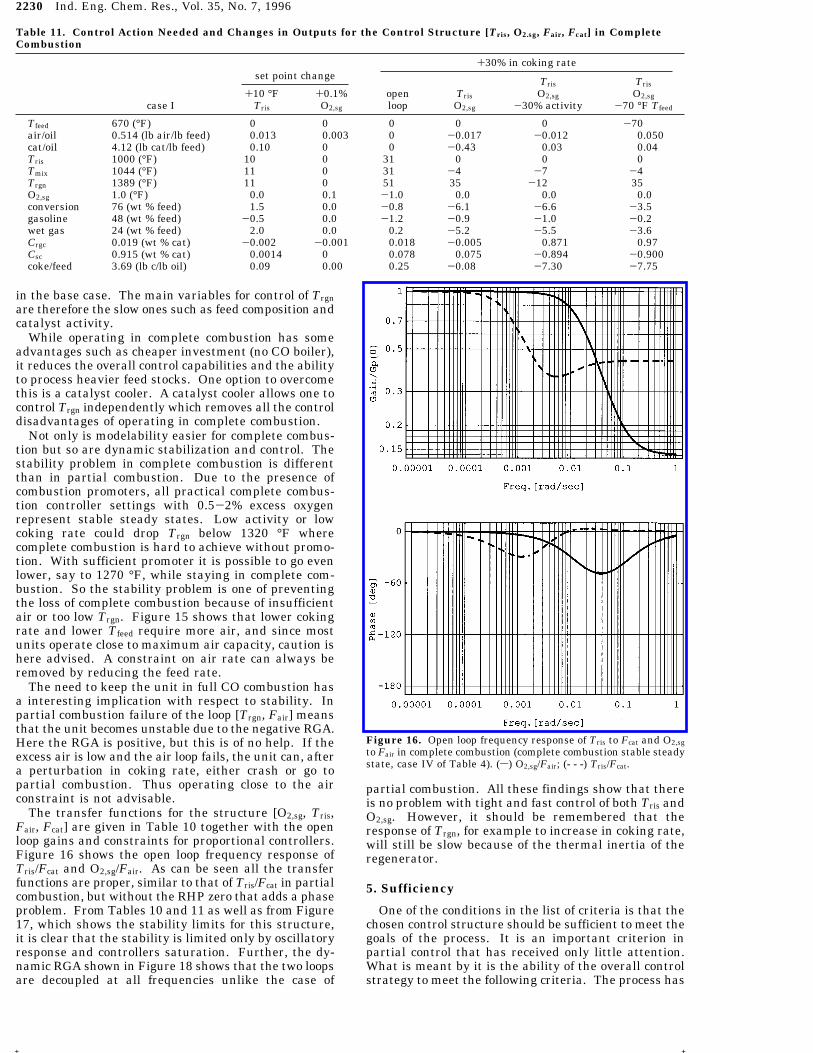
Fair, Fcat] are given in Table 10 together with the openloop gains and constraints for proportional controllers.Figure 16 shows the open loop frequency response ofTris/Fcat and O2,sg/Fair. As can be seen all the transferfunctions are proper, similar to that of Tris/Fcat in partialcombustion, but without the RHP zero that adds a phaseproblem. From Tables 10 and 11 as well as from Figure17, which shows the stability limits for this structure,it is clear that the stability is limited only by oscillatoryresponse and controllers saturation. Further, the dy-namic RGA shown in Figure 18 shows that the two loopsare decoupled at all frequencies unlike the case of
partial combustion. All these findings show that thereis no problem with tight and fast control of both Tris andO2,sg. However, it should be remembered that theresponse of Trgn, for example to increase in coking rate,will still be slow because of the thermal inertia of theregenerator.
5. Sufficiency
One of the conditions in the list of criteria is that thechosen control structure should be sufficient to meet thegoals of the process. It is an important criterion inpartial control that has received only little attention.What is meant by it is the ability of the overall controlstrategy to meet the following criteria. The process has
Table 11. Control Action Needed and Changes in Outputs for the Control Structure [Tris, O2.sg, Fair, Fcat] in CompleteCombustion
Figure 16. Open loop frequency response of Tris to Fcat and O2,sgto Fair in complete combustion (complete combustion stable steadystate, case IV of Table 4). (s) O2,sg/Fair; (- - -) Tris/Fcat.
to be able to keep Yp within the specified goals and todeal with the perturbations expected to occur in aneconomical acceptable way. Yp is imposed from theoutside. But in determining it one has to take intoaccount the capabilities of the process. The ability ofany control structure to achieve these goals is deter-mined in the plant design as it depends not only on thedesign of the process but also on the number andmagnitude of the manipulated variables provided in theoriginal design. It is therefore important to understandwhat sufficiency means and how the ability to providea sufficient control structure depends on the design.During the early years (1938) of FCC operation anyproduct coming out of it was acceptable, and there arestill plants for which this is so. Today the specificationson gasoline have become much tighter due to environ-mental considerations. This and the need to crackheavier feed stocks give an economical advantage tounits with a greater capability for control.Those units that are limited in their ability to
manipulate catalyst circulation rate have an economicpenalty as one cannot control Tris and Trgn indepen-dently. Much of the development in FCC technologysuch as feed preheat, catalyst cooler, and the slide valvefor controlling Fcat has been motivated by the need toprovide better controllability. The section on control ofcomplete combustion is a good illustration. While in
complete combustion a 2 × 2 control matrix is usedsimilar to partial combustion, the ability to control Ypand to deal with heavier feeds is much more limited, adisadvantage that has to be weighted against the costadvantages of the unit. While for some needs thiscontrol structure is sufficient for achieving the demandgoals, changing needs may justify the conversion of theunit to partial combustion, just as some other units,such as the Model IV, are being converted to allowcontrol of Fcat with a slide valve. There are otherindustries in which specifications imposed from theoutside are much tighter than in refining. There theneed to ensure sufficiency of the control structure tomeet Yp is a much more urgent concern, but the examplegiven here still illustrates the concept.
6. Summary
The goal of this paper was to set forward in moredetail the concepts of partial control or, in other words,the control of complex systems with a limited choice ofmanipulated inputs. The approach was illustrated bydescribing in detail the choice of a control structure foran FCC. It was shown that despite its complexity anFCC can be quite well controlled and stabilized by a 2× 2 control structure. This primary structure filtersdisturbances and keeps the system stable.The role of the dynamic control structure is much
more than just to stabilize the system and filterdisturbances. It plays a key role in steady state control,which relies not only on changing the set points of the2 × 2 control structure but also on a number of othermanipulated inputs which are called slow control loops.The dynamic control structure chosen has therefore
to take into account the role in the overall controlstrategy. Criteria to do so were defined in Table 1. Asan example four dynamic control structures that werediscussed in the literature before (Hovd and Skogestad,1992, 1993; Balchen et al., 1992 and others) wereevaluated in detail to demonstrate the approach, andthe role of the slow manipulated variables in the overallcontrol strategy was shown by examples.The method outlined in the paper should be generally
useful for a wide variety of complex nonlinear processes.However, as the constraints and properties of suchsystems vary considerably, design will always be aquestion of judgment, compromise, and choice. It ishard to develop a general algorithmic approach. Rosen-brook (1974) has pointed out that this applies not onlyto partial control but also to proper controller design.The example of the FCC given here shows however quiteclearly how one analyzes the different criteria in Table1 and how they impact on the design.There are several general results that apply to the
FCC and that should be of wide interest as they appearin many other cases:1. One cannot judge the suitability of any control
structure by analyzing only the performance of themeasured variables used for the set points, but one hasto look at the behavior of all variables entering thespecifications. Therefore, one cannot design a controlstructure solely based on a model as the specificationsstrongly impact on the design. This implies that it ishard to provide a generalized algorithm for controldesign.2. A control structure useful in one domain of
operation (here partial combustion) may be totallyunsuitable for a different operating domain (here com-plete combustion).
Figure 17. Stability limits for the control structure [(O2,sg, Fair),(Tris, Fcat)] at case IV of Table 4 (stable steady state in completecombustion) with P and PI controller: Ki (1 + 0.001/s).
Figure 18. Dynamic RGA for the control structure [Tris, O2,sg,Fair, Fcat] (all conditions are of case IV of Table 4). (s) Maindiagonal: [(O2,sg, Fair), (Tris, Fcat)]; (- - -) Off diagonal: [(O2,sg, Fcat),(Tris, Fair)].
3. In the FCC linear algorithms are satisfactory fortuning control loops. The main impact of nonlinearityis on the choice of the primary structure itself, on steadystate control of set points, and on delineating theoperating domain in which a control system can func-tion. Nonlinear dynamic control can here contributevery little. This is of special importance as presentacademic research in process control focusses on non-linear dynamic control which very seldom has a signifi-cant impact and is in most cases of far smaller impor-tance than the nonlinear problems outlined here.4. The sufficiency of a control structure to allow the
process to achieve the goals imposed on it by the spe-cifications and changing market requirements stronglydepends on the design of the process. This is oftenneglected in the design of new processes. In a futurepaper we will discuss these problems as they effect theFCC.The problems of partial control have been discussed
in an heuristic way. Considerable further research isneeded to fully understand the problems involved insteady state control of chemical plants and othercomplex processes. It is our hope that this paper willstimulate such work.
Acknowledgment
This work was supported by the Division of BasicEnergy Sciences of the Department of Energy underGrant No. DE-FG02-91-ER14221. The authors want toacknowledge their gratitude for this support. Theauthors also wish to thank Prof. Manfred Morari of ETHin Zurich as well as Dr. Amos Avidan and Dr. Ajit Sapreof Mobil for many helpful discussions and comments.
Nomenclature
∆T ) temperature rise from the regenerator dense bed tothe stack gas [°F]
ε ) riser bed void fractionFc ) catalyst density [lb/ft3]τr ) residence time in the riser [s]φ ) deactivation function (see eq A-4 in Arbel et al., 1995a)A ) Relative catalyst activityaik ) stoichiometric coefficient between lump i and kair/oil ) air flow rate to feed flow rate ratio (FairMWair/Ffeed) [lb air/lb feed]
cat/oil ) catalyst flow rate to feed flow rate ratio (Fcat/Ffeed)[lb cat/lb feed]
conv ) conversion [wt %]Crgc ) coke on regenerated catalyst [wt %]Csc ) coke on spent catalyst [wt %]Ek ) cracking rate of lump k activation energy [Btu/lb mol]Fair ) air flow rate to the regenerator [mol/s]Fcat ) catalyst circulation rate [lb/s]Ffeed ) oil feed flow rate [lb/s]Gcd ) primary dynamic control strategyGs ) steady state control strategyh ) dimensionless riser heightkh ) adsorption of heavy aromatics rate constantKk0 ) cracking rate of lump k pre-exponential coefficientM ) reduced order nonlinear model of a processM* ) full order unknown nonlinear model of a processN ) unknown and unmeasured inputs (disturbances)O2,sg ) oxygen in stack gas [mol %]R ) gas law constantTfeed ) oil feed temperature [°F]Tmix ) temperature at the riser bottom after feed andcatalyst mix [°F]
Trgn ) regenerator dense bed temperature [°F]Tris ) riser top temperature [°F]
Tsg ) stack gas temperature [°F]U ) vector of manipulated inputsUcd ) subvector of manipulated inputs entering the pri-mary control
Ud ) subvector of manipulated inputs that can be variedfast
Us ) subvector of manipulated inputs that can be variedslow
Uss ) vector of settings for the inputs at steady stateW ) vector of measured but not manipulated inputsX ) reduced order vector of state variablesX* ) full order vector of state variablesY ) vector of outputsYcd ) subvector of outputs entering the primary controlYd ) subvector of outputs measured frequentlyYg ) gasoline yield [wt %]yi ) (in eq 6 only) weight fraction of lump i in the oil feedor product
Yp ) subvector of outputs defining specifications andconstraints
Ys ) subvector of outputs measured less frequentlyYss
Arbel, A.; Huang, Z.; Rinard, I. H.; Shinnar, R.; Sapre, A. V.Dynamic and Control of Fluidized Catalytic Crackers. 1. Model-ing of the Current Generation of FCC’s. Ind. Eng. Chem. Res.1995a, 34, 1228-1243.
Arbel, A.; Rinard, I. H.; Shinnar, R.; Sapre, A. V. Dynamic andControl of Fluidized Catalytic Crackers. 2. Multiple SteadyStates and Instabilities. Ind. Eng. Chem. Res. 1995b, 34, 3014-3026.
Aris, R. Mathematical Modelling; Pitman: Boston, MA, 1978.Avidan, A. A.; Shinnar, R. Development of Catalytic CrackingTechnology. A Lesson in Chemical Reactor Design. Ind. Eng.Chem. Res. 1990, 29, 931-942.
Balchen, J. G.; Ljungquist, D.; Strand, S. State Space PredictiveControl. Chem. Eng. Sci. 1992, 47, 787-807.
Bristol, E. H. On a NewMeasure of Interactions for MultivariableProcess Control. IEEE Trans. Automat. Control 1966, AC-11,133.
Cutler, C. R.; Ramaker, B. L. Dynamic Matrix Control - AComputer Control Algorithm. Proceedings of the AutomaticControl Conference; San Francisco, CA, 1980; Paper WP5-B.
Denn, M. Process Modelling; W. H. Freeman: New York, 1986.Edwards, W. M.; Kim, H. N. Multiple Steady States in FCCUOperations. Chem. Eng. Sci. 1988, 43, 8, 1825-1830.
Hovd, M.; Skogestad, S. Controllability Analysis for the FluidCatalytic Cracking Process. Ind. Eng. Chem. Res. 1992, 31,1589.
Hovd, M.; Skogestad, S. Procedure for Regulatory Control Struc-ture Selection with Application to the FCC Process. AIChE J.1993, 39 (12), 1938-1953.
Hovd, M.; Skogestad, S. Pairing Criteria for Decentralized Controlof Unstable Plants. Ind. Eng. Chem. Res. 1994, 33, 2134-2139.
Huq, I.; Morari, M.; Sorensen, R. C. Design of operationalModification to Model IV FCCUs to Improve Dynamic Perfor-mance. AIChE J. 1995, 4, 1481-1499.
Kokotovic, P. V.; O’Malley, R. E., Jr.; Sannuti, P. SingularPertubations and Order Reduction in Control TheorysAnOverview. Automatica 1976, 12, 123-132.
Kurihara, H. Optimal Control of Fluid Catalytic Cracking Process.Ph.D. Dissertation, MIT, MI, 1967.
Martinez, E. C.; Drozdowicz, B. Multiple-Scale Approach to Real-Time Simulation of Stiff Dynamic Systems.Comput. Chem. Eng.1989, 13, 7, 767-778.
McAvoy, T. J. Interaction Analysis. Instrument Society of America:Research Triangle Park, NC, 1983.
Meadowcroft, T. A.; Stephanopoulos, G.; Brosilow, C. The ModularMultivariable Controller: I: Steady-State properties. AIChE J.1992, 38, 8, 1254-1278.
2232 Ind. Eng. Chem. Res., Vol. 35, No. 7, 1996
+ +
Morari, M. Robust Stability of System with Integral Control. IEEE22nd CDC 1985, 865-869.
Morari, M.; Zafiriou, E. Robust Process Control; Prentice-Hall:Englewood Cliffs, NJ, 1989.
Morari, M.; Arkun, Y; Stephanopolous, G. Studies in the Synthesisof Control Structure for Chemical Processes, Part I, II and III.AIChE J. 1982, 28, 60.
Prett, D. M.; Garcia, C. E. Fundamental Process Control; Butter-worth: Stoneham, MA, 1988.
Rosenbrook, H. H. Computer-Aided Control System Design; Aca-demic Press: London, 1974.
Shinnar, R. The Interface Between Industry and the AcademicWorld. AIChE Symp. Ser. 1976, 159, 72, 155-166.
Shinnar, R. Chemical Reactor Modeling. The Desirable and theAchievable. Chem. React. Eng. Rev. 1978, 29, 1-36.
Shinnar, R. Chemical Reactor Modelling for the Purposes ofController Design. Chem. Eng. Commun. 1981, 9, 73-99.
Shinnar, R. Impact of Model Uncertainties and Nonlinearities onModern Controller Design. Present Status and Future Goals.In Chemical Process Control-CPCIII, Proceedings of the 3rd
International Conference on Chemical Process Control; Morari,M., McAvoy, T. J., Eds.; Elsvier: New York, 1986; pp 53-93.
Shinseky, F. G. Process Control Systems; McGraw Hill: New York,1967.
Shinseky, F. G. Distillation Column Control, 2nd ed.; McGrawHill: New York, 1984.
Silverstein, J.; Shinnar, R. The Effect of Design on the Stabilityand Control of Fixed Bed Catalytic Reactors with Heat Feed-back 1. Concepts. In Ind. Eng. Chem. Process Des. Dev. 1982,21, 241-256.
Received for review November 28, 1995Accepted April 24, 1996X
IE9507080
X Abstract published in Advance ACS Abstracts, June 15,1996.