60
Dynamics and control of incineration processes Davide Manca Lesson 2 of “Dynamics and Control of Chemical Processes” – Master Degree in Chemical Engineering

© Davide Manca – Dynamics and Control of Chemical Processes – Master Degree in ChemEng – Politecnico di Milano 1L2—
Dynamics and control of incineration processes
Davide Manca
Lesson 2 of “Dynamics and Control of Chemical Processes” – Master Degree in Chemical Engineering
© Davide Manca – Dynamics and Control of Chemical Processes – Master Degree in ChemEng – Politecnico di Milano 2L2—
Table of contents
Implementation and validation of a detailed first-principles
dynamic model of the combustion section of an incineration plant
Analysis of a multivariable MPC control system
Model reduction
Synthesis of a non-linear MPC control system
Identification of an ARX linear model
Synthesis of a linear MPC control system and comparison with
the non-linear counterpart

© Davide Manca – Dynamics and Control of Chemical Processes – Master Degree in ChemEng – Politecnico di Milano 3L2—
Hot section of an incineration plant
Primary kiln
Economizer
Superheater
Boiler
Postcombustion chamber

© Davide Manca – Dynamics and Control of Chemical Processes – Master Degree in ChemEng – Politecnico di Milano 4L2—
Grate kiln
© Davide Manca – Dynamics and Control of Chemical Processes – Master Degree in ChemEng – Politecnico di Milano 5L2—
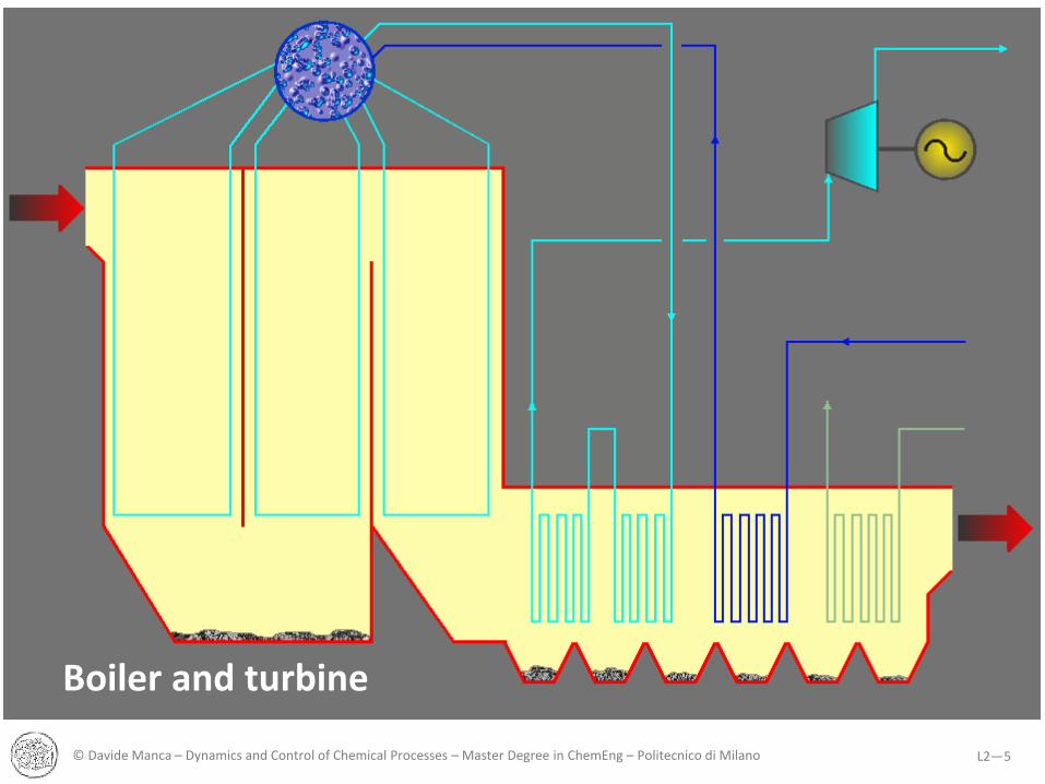
Boiler and turbine

© Davide Manca – Dynamics and Control of Chemical Processes – Master Degree in ChemEng – Politecnico di Milano 6L2—
Fabric filter and exhaust gas washing

© Davide Manca – Dynamics and Control of Chemical Processes – Master Degree in ChemEng – Politecnico di Milano 7L2—
DeNOx and Catox

© Davide Manca – Dynamics and Control of Chemical Processes – Master Degree in ChemEng – Politecnico di Milano 8L2—
Layout of an incineration plant

© Davide Manca – Dynamics and Control of Chemical Processes – Master Degree in ChemEng – Politecnico di Milano 9L2—
Primary combustion chamber

© Davide Manca – Dynamics and Control of Chemical Processes – Master Degree in ChemEng – Politecnico di Milano 10L2—

© Davide Manca – Dynamics and Control of Chemical Processes – Master Degree in ChemEng – Politecnico di Milano 11L2—
Primary kiln – Modeling scheme
1
2
2.1
2.2
2.3
2.4
2.5
3.1 3.2 3.3 3.4
4
Homogenous combustion zone
Heterogeneous combustion zone
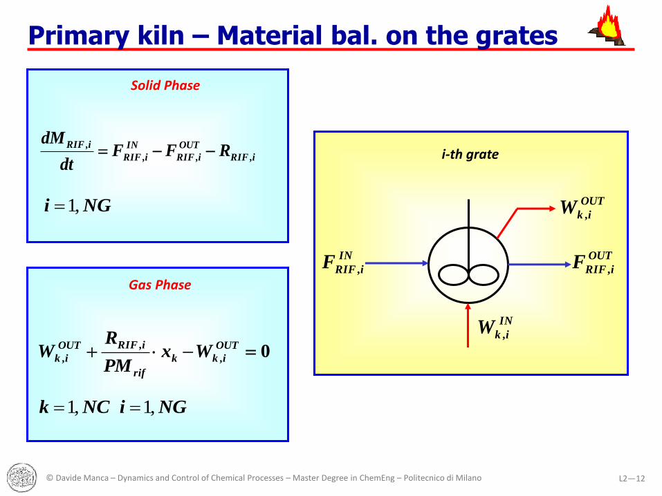
© Davide Manca – Dynamics and Control of Chemical Processes – Master Degree in ChemEng – Politecnico di Milano 12L2—
i,RIF
OUT
i,RIF
IN
i,RIF
i,RIFRFF
dt
dM
Solid Phase
Gas Phase
0 OUT
i,kk
rif
i,RIFOUT
i,k WxPM
RW
NGiNCk ,1,1
OUT
i,RIFFIN
i,RIFF
OUT
i,kW
IN
i,kW
i-th grate
NGi ,1
Primary kiln – Material bal. on the grates

© Davide Manca – Dynamics and Control of Chemical Processes – Master Degree in ChemEng – Politecnico di Milano 13L2—
OHkm
Nxy
NOxpSOkHClnCONClOSHCi
iykqpmn
iO
22222
,2
yx i,NOi
1
3150
25001
2
2
100
out
i,OG
%
i,NOG
i,NO
i,NO
W)T/exp(T
W
Combustion reaction in the solid phase
(Bowman, 1975)
2 2
1CO O CO
2
2 2
1 1N O NO
2 2
Combution reactions in the gas phase
Kinetics

© Davide Manca – Dynamics and Control of Chemical Processes – Master Degree in ChemEng – Politecnico di Milano 14L2—
, , , ,( , , , )sc i p i i waste i inerts iA f d M M
)exp(11
,
iCG
i
Nisciisc AA ,
*
,
2
2
, , *
, ,
,
x i O i
waste i sc i waste
O i
k xR A PM
Corrective factor with adaptive parameters
),,,,( ,,,, TxWdfk ikiariaiipix Solid granular bed
Kinetic determining step: O2 diffusion
,
2 ,O i see L2–18 eq. (8)
Primary kiln – Combustion kinetics

© Davide Manca – Dynamics and Control of Chemical Processes – Master Degree in ChemEng – Politecnico di Milano 15L2—
x
h
b
wastem x b h
Grate schematization
© Davide Manca – Dynamics and Control of Chemical Processes – Master Degree in ChemEng – Politecnico di Milano 16L2—
Fw
aste (t
) [k
g/s]
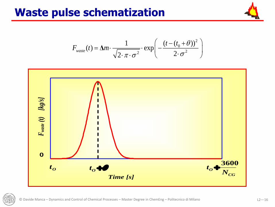
0
Ot
Ot
CG
ON
t3600
Time [s]
2
0
22
1 ( ( ))( ) exp
22waste
t tF t m
Δ
Waste pulse schematization
© Davide Manca – Dynamics and Control of Chemical Processes – Master Degree in ChemEng – Politecnico di Milano 17L2—
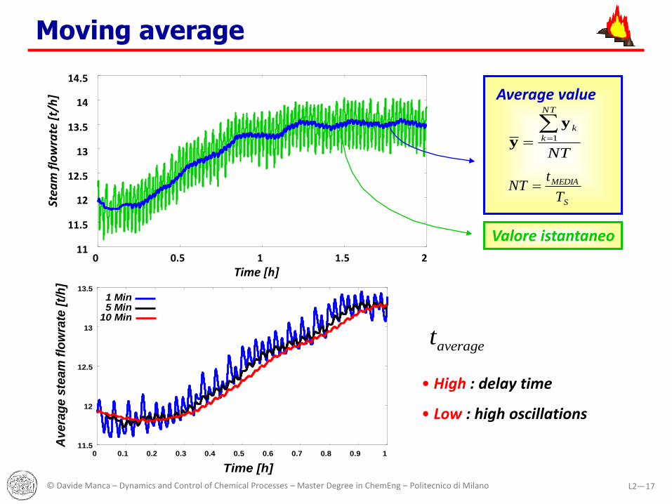
11
11.5
12
12.5
13
13.5
14
14.5
0 0.5 1 1.5 2
Stea
m f
low
rate
[t/
h]
Time [h]
Average value
NT
NT
k
k 1
y
y
S
MEDIA
T
tNT
Valore istantaneo
11.5
12
12.5
13
13.5
0 0.1 0.2 0.3 0.4 0.5 0.6 0.7 0.8 0.9 1
Avera
ge s
team
flo
wra
te [
t/h
]
Time [h]
1 Min 5 Min
10 Min
• High : delay time
• Low : high oscillations
averaget
Moving average
© Davide Manca – Dynamics and Control of Chemical Processes – Master Degree in ChemEng – Politecnico di Milano 18L2—
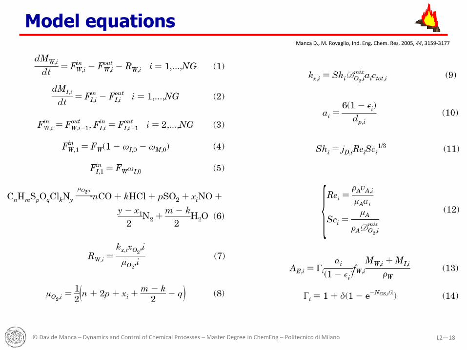
Manca D., M. Rovaglio, Ind. Eng. Chem. Res. 2005, 44, 3159-3177
Model equations

© Davide Manca – Dynamics and Control of Chemical Processes – Master Degree in ChemEng – Politecnico di Milano 19L2—
Manca D., M. Rovaglio, Ind. Eng. Chem. Res. 2005, 44, 3159-3177
Model equations

© Davide Manca – Dynamics and Control of Chemical Processes – Master Degree in ChemEng – Politecnico di Milano 20L2—
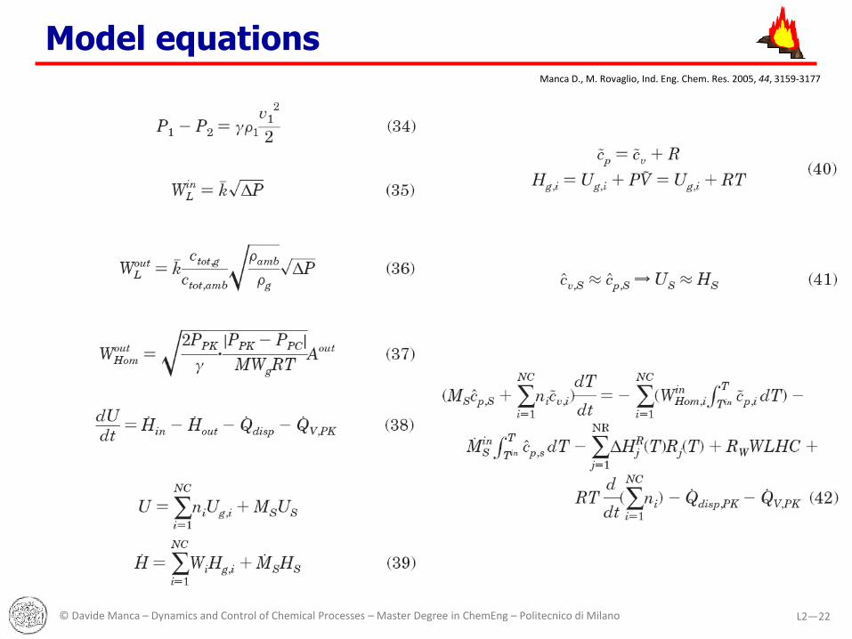
Manca D., M. Rovaglio, Ind. Eng. Chem. Res. 2005, 44, 3159-3177
Model equations

© Davide Manca – Dynamics and Control of Chemical Processes – Master Degree in ChemEng – Politecnico di Milano 21L2—
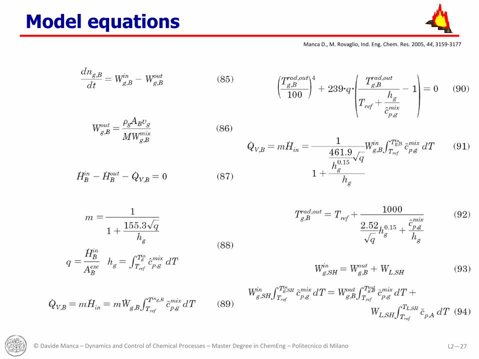
Manca D., M. Rovaglio, Ind. Eng. Chem. Res. 2005, 44, 3159-3177
Model equations
© Davide Manca – Dynamics and Control of Chemical Processes – Master Degree in ChemEng – Politecnico di Milano 22L2—
Manca D., M. Rovaglio, Ind. Eng. Chem. Res. 2005, 44, 3159-3177
Model equations

© Davide Manca – Dynamics and Control of Chemical Processes – Master Degree in ChemEng – Politecnico di Milano 23L2—
Manca D., M. Rovaglio, Ind. Eng. Chem. Res. 2005, 44, 3159-3177
Model equations

© Davide Manca – Dynamics and Control of Chemical Processes – Master Degree in ChemEng – Politecnico di Milano 24L2—
Manca D., M. Rovaglio, Ind. Eng. Chem. Res. 2005, 44, 3159-3177
Model equations

© Davide Manca – Dynamics and Control of Chemical Processes – Master Degree in ChemEng – Politecnico di Milano 25L2—
Manca D., M. Rovaglio, Ind. Eng. Chem. Res. 2005, 44, 3159-3177
Model equations

© Davide Manca – Dynamics and Control of Chemical Processes – Master Degree in ChemEng – Politecnico di Milano 26L2—
Manca D., M. Rovaglio, Ind. Eng. Chem. Res. 2005, 44, 3159-3177
Model equations
© Davide Manca – Dynamics and Control of Chemical Processes – Master Degree in ChemEng – Politecnico di Milano 27L2—
Manca D., M. Rovaglio, Ind. Eng. Chem. Res. 2005, 44, 3159-3177
Model equations

© Davide Manca – Dynamics and Control of Chemical Processes – Master Degree in ChemEng – Politecnico di Milano 28L2—
Manca D., M. Rovaglio, Ind. Eng. Chem. Res. 2005, 44, 3159-3177
<
Model equations

© Davide Manca – Dynamics and Control of Chemical Processes – Master Degree in ChemEng – Politecnico di Milano 29L2—
Materialbalances
Energy balances
Momentumbalances
Total
Primary kinl
29 2 86
Postcombustion chamber 15 1 26
Heat recoverysection
55
10
6 9 5 20
Grand total = 132 DAE system
Model dimensions in terms of DAEs

© Davide Manca – Dynamics and Control of Chemical Processes – Master Degree in ChemEng – Politecnico di Milano 30L2—
Number of feed-strokes [1/h] 40
Inlet waste flowrate [kg/h] 4,000
Number of strokes to the first grate [1/h] 23
Number of strokes to the second grate [1/h] 20
Number of strokes to the third grate [1/h] 13
Number of strokes to the fourth grate [1/h] 23
Primary air flowrate [Nm3/h] 12,500
Secondary air flowrate [Nm3/h] 6,500
Some significant input process variables
Outlet smokes temperature from the primary kiln [°C] 1,035
Outlet smokes temperature from the postcombustion chamber [°C] 1,115
Outlet oxygen molar fraction from the postcombustion chamber [%] 8.5
Outlet CO content from the postcombustion chamber [mg/Nm3] 11
Steam flowrate [t/h] 12
Some significant output process variables
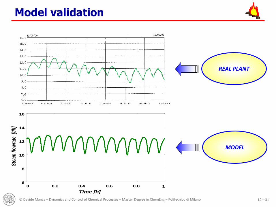
© Davide Manca – Dynamics and Control of Chemical Processes – Master Degree in ChemEng – Politecnico di Milano 31L2—
REAL PLANT
6
8
10
12
14
16
0 0.2 0.4 0.6 0.8 1
Ste
am fl
owra
te [
t/h]
Time [h]
MODEL
Model validation

© Davide Manca – Dynamics and Control of Chemical Processes – Master Degree in ChemEng – Politecnico di Milano 32L2—
3400
3600
3800
4000
4200
4400
4600
4800
11 12 13 14 15 16 17
Po
rtata
di ri
fiu
to [
kg
/h]
Tempo [h]
3000
3500
4000
4500
5000
5500
6000
6500
11 12 13 14 15 16 17 Po
rtata
di ari
a s
eco
nd
ari
a [
Nm
3/h
]
Tempo [h]
9600
9900
10200
10500
10800
11100
11400
11700
12000
12300
12600
11 12 13 14 15 16 17
Po
rtata
di ari
a a
lle g
rig
lie [
Nm
3/h
]
Tempo [h]
10200
10400
10600
10800
11000
11200
11400
11600
11800
12000
12200
12400
11 12 13 14 15 16 17 Po
tere
calo
rifi
co
del ri
fiu
to [
kJ/k
g]
Tempo [h]
9
10
11
12
13
14
15
16
11 12 13 14 15 16 17
Po
rta
ta v
ap
ore
[t/
h]
Tempo [h]
REAL INPUTS
SIMULATED OUTPUT
DYNAMIC SIMULATOR
Model validation
© Davide Manca – Dynamics and Control of Chemical Processes – Master Degree in ChemEng – Politecnico di Milano 33L2—
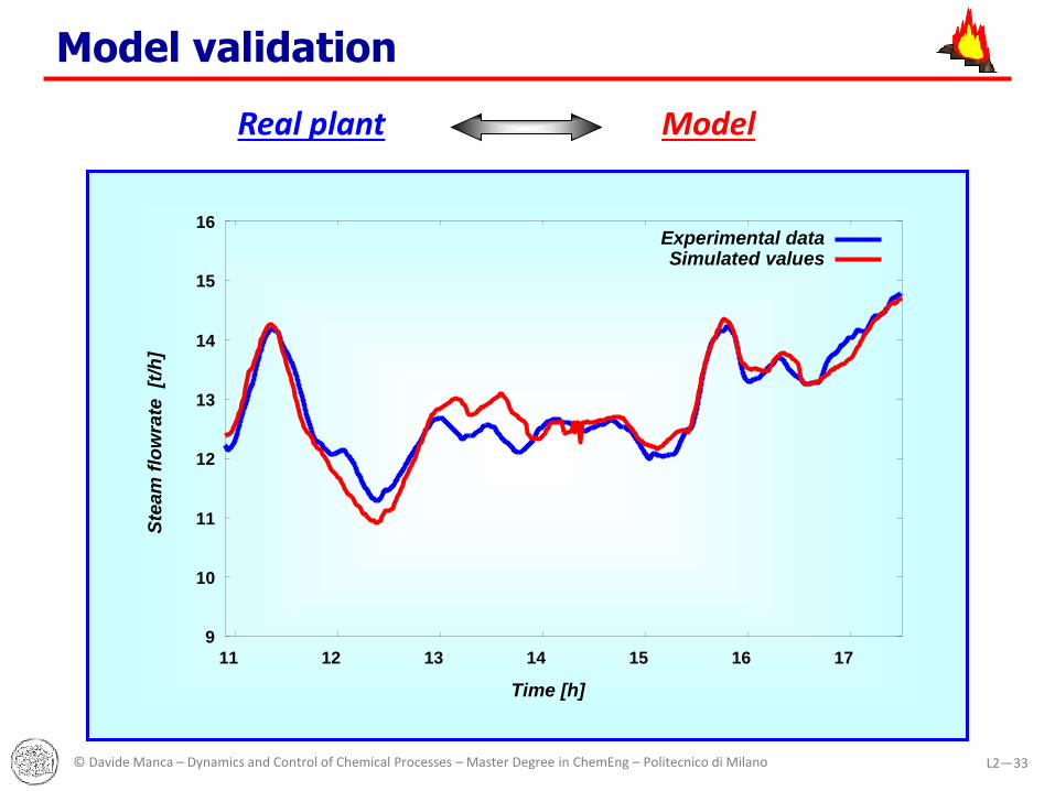
9
10
11
12
13
14
15
16
11 12 13 14 15 16 17
Ste
am
flo
wra
te
[t/h
]
Time [h]
Experimental data Simulated values
ModelReal plant
Model validation
© Davide Manca – Dynamics and Control of Chemical Processes – Master Degree in ChemEng – Politecnico di Milano 34L2—
Experimental data
Simulated values
940
960
980
1000
1020
1040
1060
1080
1100
1120
1140
1160
11 12 13 14 15 16 17
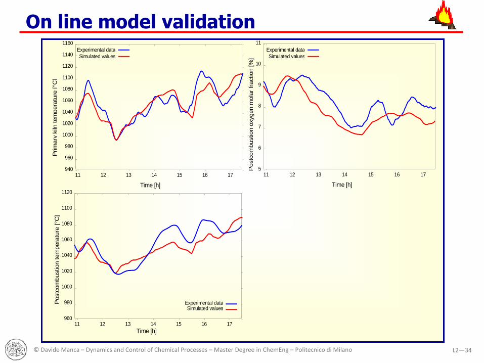
Prim
ary
kiln tem
pera
ture
[°C
]
Time [h]
5
6
7
8
9
10
11
11 12 13 14 15 16 17
Time [h]
Postc
om
bustion o
xygen m
ola
r fr
action [%
]
960
980
1000
1020
1040
1060
1080
1100
1120
11 12 13 14 15 16 17
Experimental data Simulated values
Postc
om
bustion tem
pera
ture
[°C
]
Time [h]
Experimental data
Simulated values
On line model validation
© Davide Manca – Dynamics and Control of Chemical Processes – Master Degree in ChemEng – Politecnico di Milano 35L2—
600
700
800
900
1000
1100
1200
1300
1400
1500
1600
11 12 13 14 15 16 17
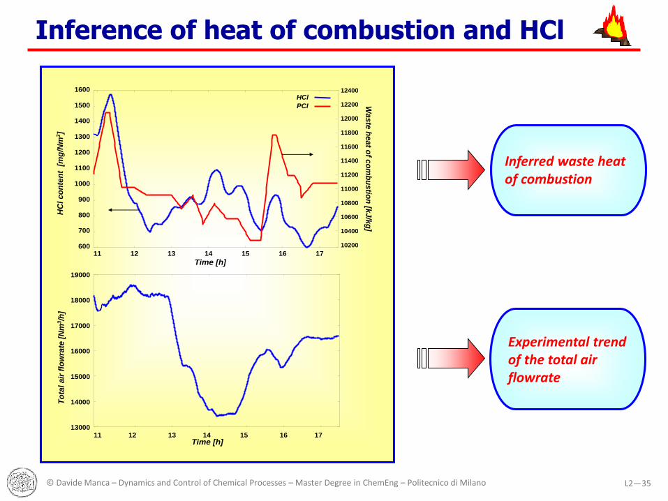
HCl
PCI
Wa
ste
he
at o
f co
mb
us
tion
[kJ/k
g]
HC
l c
on
ten
t [
mg
/Nm
3]
Time [h]
10200
10400
10600
10800
11000
11200
11400
11600
11800
12000
12200
12400
13000
14000
15000
16000
17000
18000
19000
11 12 13 14 15 16 17
To
tal
air
flo
wra
te [
Nm
3/h
]
Time [h]
Inferred waste heat of combustion
Experimental trend of the total air flowrate
Inference of heat of combustion and HCl

© Davide Manca – Dynamics and Control of Chemical Processes – Master Degree in ChemEng – Politecnico di Milano 36L2—
6
8
10
12
14
16
0 0.2 0.4 0.6 0.8 1
Stea
m f
low
rate
[t
/h]
Time [h]
Dynamic response to different forcing actions
6
8
10
14
16
0 0.2 0.4 0.6 0.8 1
Stea
m f
low
rate
[t/
h]
Time [h]
12
3 x N
1 x 3N

© Davide Manca – Dynamics and Control of Chemical Processes – Master Degree in ChemEng – Politecnico di Milano 37L2—
Multivariable model based
control

© Davide Manca – Dynamics and Control of Chemical Processes – Master Degree in ChemEng – Politecnico di Milano 38L2—
Implementation and validation of a detailed first-principles
dynamic model of the combustion section of an incineration plant
Analysis of a multivariable MPC control system
Model reduction
Synthesis of a non-linear MPC control system
Identification of an ARX linear model
Synthesis of a linear MPC control system and comparison with
the non-linear counterpart
Table of contents

© Davide Manca – Dynamics and Control of Chemical Processes – Master Degree in ChemEng – Politecnico di Milano 39L2—
Use of a model for predictive pursposes
sety
+
Model+
Constraints
Optimizer
Model
Process
+
-
+
-
-
d
y
y
y
u
u
MPC – Implementation scheme
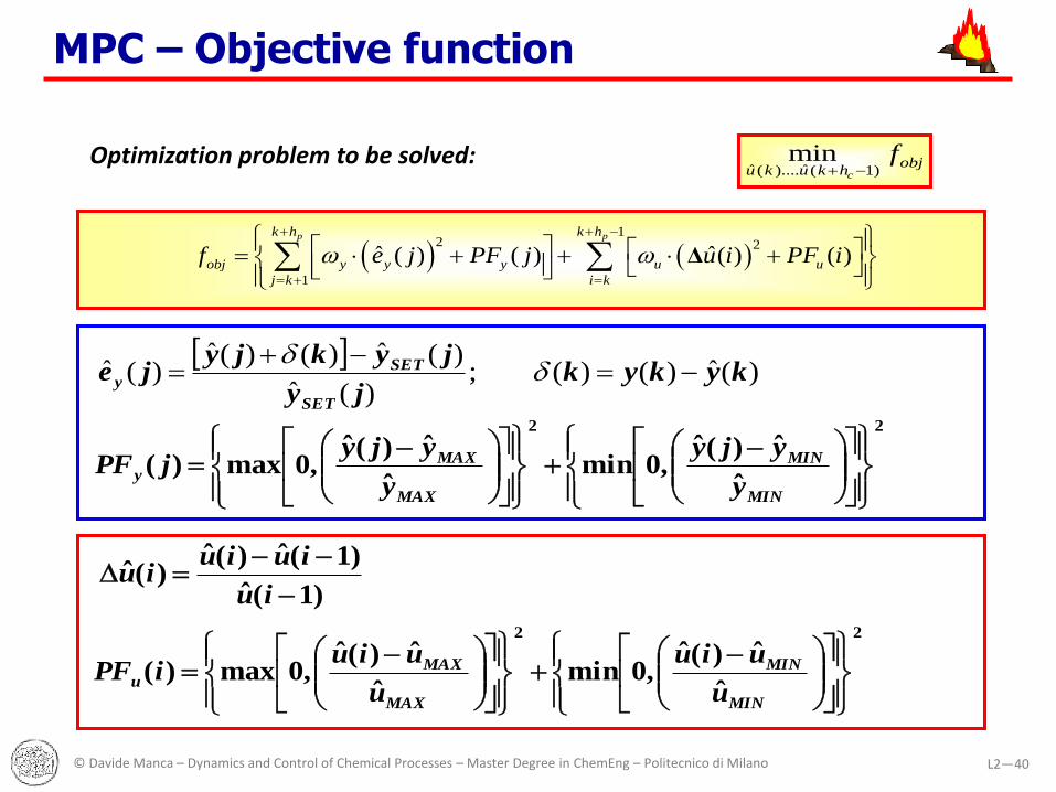
© Davide Manca – Dynamics and Control of Chemical Processes – Master Degree in ChemEng – Politecnico di Milano 40L2—
ˆ ˆ( ).... ( 1)min
cobj
u k u k hf
1
2 2
1
ˆ ˆ( ) ( ) ( ) ( )p pk h k h
obj y y y u u
j k i k
f e j PF j u i PF i
Δ
22
ˆ
ˆ)(ˆ,0min
ˆ
ˆ)(ˆ,0max)(
MIN
MIN
MAX
MAXu
u
uiu
u
uiuiPF
)(ˆ)()(;
)(ˆ
)(ˆ)()(ˆ)(ˆ kykyk
jy
jykjyje
SET
SETy
)1(ˆ
)1(ˆ)(ˆ)(ˆ
iu
iuiuiu
Optimization problem to be solved:
22
ˆ
ˆ)(ˆ,0min
ˆ
ˆ)(ˆ,0max)(
MIN
MIN
MAX
MAXy
y
yjy
y
yjyjPF
MPC – Objective function

© Davide Manca – Dynamics and Control of Chemical Processes – Master Degree in ChemEng – Politecnico di Milano 41L2—
CONTROLLED VARIABLES (CV)
Steam flowrate (set point)
Primary kiln temperature (upper bound)
Postcombustion chamber temperature (upper bound)
Postcombustion chamber temperature(lower bound)
Volumetric O2 fraction in the postcombustion chamber (lower bound)
CO content in the postcombustion chamber (upper bound)
MPC – Controlled variables (CV)
© Davide Manca – Dynamics and Control of Chemical Processes – Master Degree in ChemEng – Politecnico di Milano 42L2—
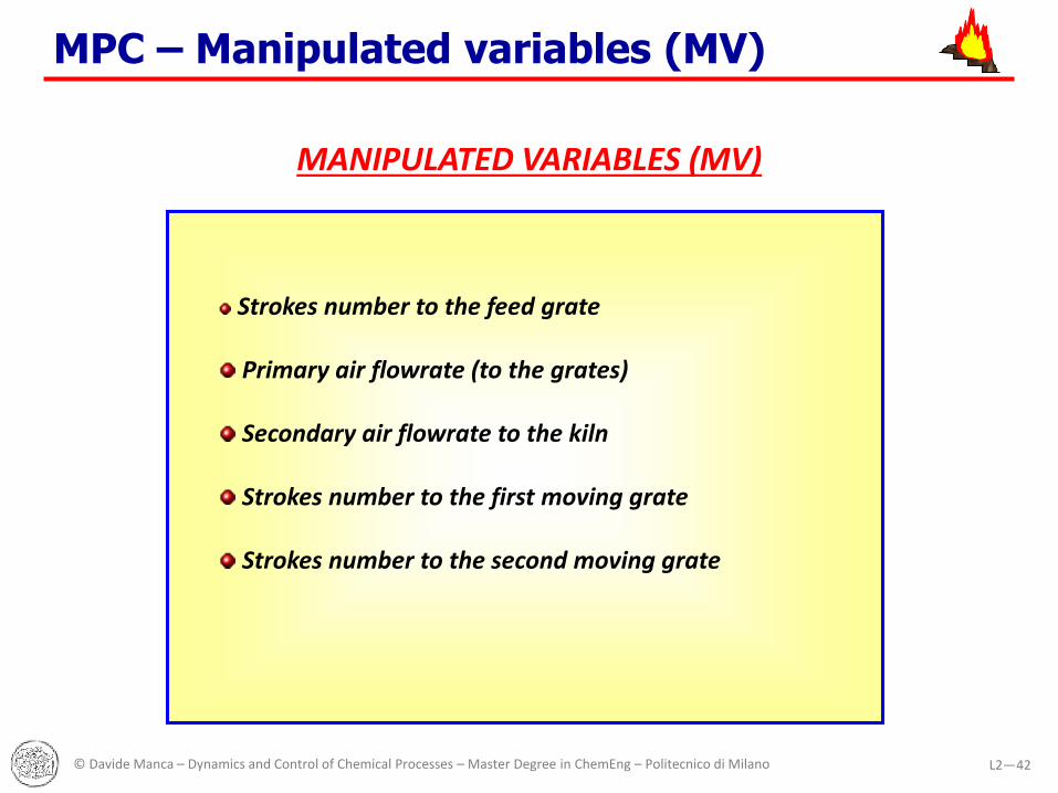
MANIPULATED VARIABLES (MV)
Strokes number to the feed grate
Primary air flowrate (to the grates)
Secondary air flowrate to the kiln
Strokes number to the first moving grate
Strokes number to the second moving grate
MPC – Manipulated variables (MV)
© Davide Manca – Dynamics and Control of Chemical Processes – Master Degree in ChemEng – Politecnico di Milano 43L2—
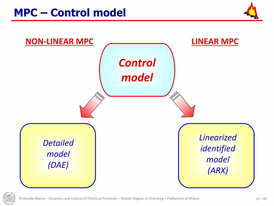
NON-LINEAR MPC LINEAR MPC
Controlmodel
Detailedmodel(DAE)
Linearizedidentified
model(ARX)
MPC – Control model

© Davide Manca – Dynamics and Control of Chemical Processes – Master Degree in ChemEng – Politecnico di Milano 44L2—
11
11.5
12
12.5
13
13.5
14
14.5
0 0.5 1 1.5 2 S
team
flo
wra
te
[t/h
]
Time [ h ]
Continuous model 132 DAE Continuous model 68 DAE
Average value of the discontinuous model
3600
2
0
22
( ( ))1exp( )
22
3600
oCG
o
tN
t
waste
CG
t t
F m
N
ΔAveraged flowrate
Same simulated average values but significantly reduced CPU times
Continuous model(132 DAE)
10% disturbance onthe waste flowrate
Discontinuous model(132 DAE) 6.02 s
2.26 s
CPU time for a 1 min simulation interval
Simplified continuous model (68 DAE)
0.54 s
NL MPC – Continuous simplified model

© Davide Manca – Dynamics and Control of Chemical Processes – Master Degree in ChemEng – Politecnico di Milano 45L2—
14.5
Time [h]
11
11.5
12
12.5
13
13.5
14
0 0.2 0.4 0.6 0.8 1
Stea
m f
low
rate
[t/
h]
(CV
)
Average valueInstantaneous value
Set point
3900
4000
4100
4200
4300
4400
4500
4600
0 0.2 0.4 0.6 0.8 1
Wa
ste
flo
wra
te [
kg/h
] (M
V)
Time [h]
Time [h]
12600
12750
12900
13050
13200
13350
13500
0 0.2 0.4 0.6 0.8 1
Air
flo
wra
te t
o t
he
gra
tes
[Nm
3 /h
] (M
V)
5700
5800
5900
6000
6100
6200
6300
6400
6500
6600
6700
6800
0 0.2 0.4 0.6 0.8 1
Seco
nd
ary
air
flo
wra
te [
Nm
3 /h
] (M
V)
Time [h]
NL MPC – Servo problem
© Davide Manca – Dynamics and Control of Chemical Processes – Master Degree in ChemEng – Politecnico di Milano 46L2—
11.5
12
12.5
13
13.5
14
14.5
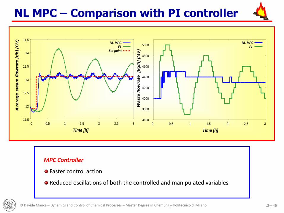
0 0.5 1 1.5 2 2.5 3
Avera
ge s
team
flo
wra
te [
t/h
] (C
V)
Time [h]
NL MPC PI
Set point
3600
3800
4000
4200
4400
4600
4800
5000
0 0.5 1 1.5 2 2.5 3
Waste
flo
wra
te
[kg
/h]
(MV
)
Time [h]
NL MPC
PI
MPC Controller
Faster control action
Reduced oscillations of both the controlled and manipulated variables
NL MPC – Comparison with PI controller
© Davide Manca – Dynamics and Control of Chemical Processes – Master Degree in ChemEng – Politecnico di Milano 47L2—
3900
4000
4100
4200
4300
4400
4500
0 0.2 0.4 0.6 0.8 1
waste
flo
wra
te [
kg
/h]
(MV
)
Time [h]
11
11.2
11.4
11.6
11.8
12
12.2
12.4
12.6
0 0.2 0.4 0.6 0.8 1
Ste
am
flo
wra
te [
t/h
] (C
V)
Time [h]
Averaged value Intstantaneous value
Set point
Time [h]
5200
5400
5600
5800
6000
6200
6400
6600
0 0.2 0.4 0.6 0.8 1 Seco
nd
ary
air
flo
wra
te [
Nm
3/h
] (M
V)
12600 12750 12900 13050 13200 13350 13500
13650 13800
13950 14100
0 0.2 0.4 0.6 0.8 1 Air
flo
wra
te t
o t
he g
rate
s [
Nm
3/h
] (M
V)
Time [h]
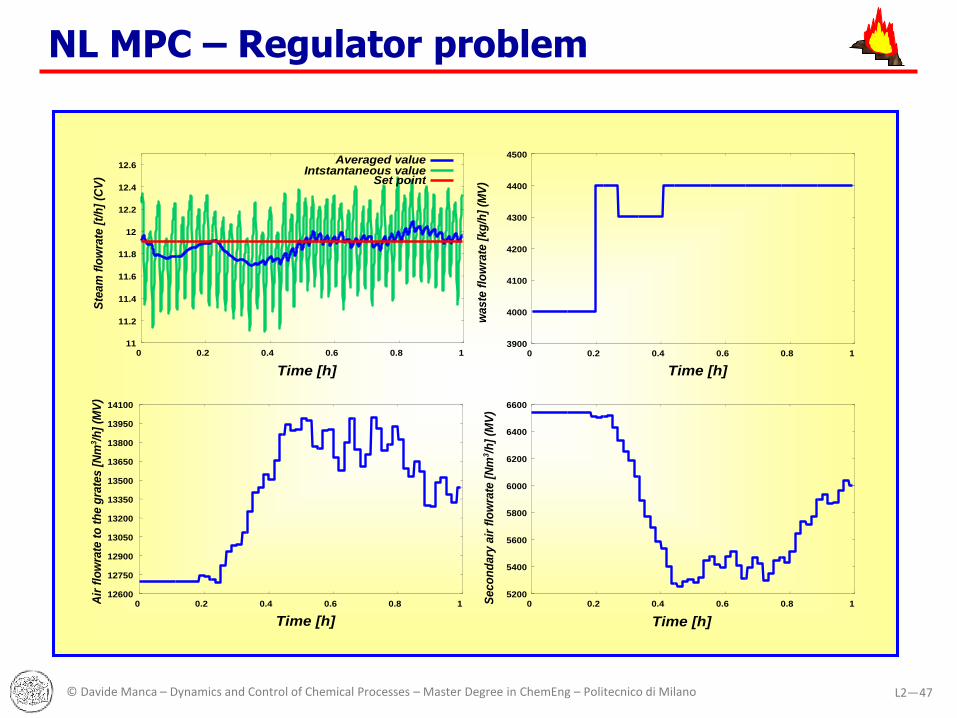
NL MPC – Regulator problem

© Davide Manca – Dynamics and Control of Chemical Processes – Master Degree in ChemEng – Politecnico di Milano 48L2—
)( tu
Plant )( ty
ARX (Auto Regressive Model with Exogenous Input )
nbknbkknaknakkk ubububyayayay 22112211
Matrix of NY·NY output parameters at time (k-i)
iky NY output vector at time (k-i)
jku NU input vector at time (k-j)
ia
jb Matrix of NY·NU input parameters at time (k-j)
na Model order respect to the outputs
nb Model order respect to the inputs
Linear MPC – ARX model

© Davide Manca – Dynamics and Control of Chemical Processes – Master Degree in ChemEng – Politecnico di Milano 49L2—
0 200 400 600 800 1000 1200 1400 1600 1800 2000 -1
-0.5
0
0.5
1
1.5
Time
Ou
tpu
t
Input and output signals
0 200 400 600 800 1000 1200 1400 1600 1800 2000 -0.04
-0.02
0
0.02
Time
Inp
ut
1000 1100 1200 1300 1400 1500 1600 1700 1800 1900 2000 -1
-0.5
0
0.5
1
1.5
Time
Measured and simulated model output
PRBS Input (Pseudo Random Binary Sequence)
MATLABSYSTEM
IDENTIFICATIONTOOLBOX
LINEAR MODELARX
Linear MPC – Identification procedure

© Davide Manca – Dynamics and Control of Chemical Processes – Master Degree in ChemEng – Politecnico di Milano 50L2—
12
12.5
13
13.5
0 0.5 1 1.5 2
Time [h]
Continuous model Linear model
Ste
am
flo
wra
te [
t/h
]
Similar trends within theprediction horizon
CPU times getsignificantly reduced
hp
Linear model (ARX)
10% disturbance on thewaste flowrate
Simplified continuousmodel (68 DAE)
0.54s
4.E-5s
CPU time for a 1 min simulation interval
Linear MPC – Models comparison

© Davide Manca – Dynamics and Control of Chemical Processes – Master Degree in ChemEng – Politecnico di Milano 51L2—
11
11.5
12
12.5
13
13.5
14
0 0.2 0.4 0.6 0.8 1
Avera
ge s
team
flo
wra
te [
t/h
] (C
V)
Time [h]
Linear MPC Set point
Non-linear MPC
Comparison between linear and non-linear MPC
The non-linear MPCreaches the
setpoint faster
Linear MPC – Servo problem

© Davide Manca – Dynamics and Control of Chemical Processes – Master Degree in ChemEng – Politecnico di Milano 52L2—
11.4
11.6
11.8
12
12.2
12.4
0 0.2 0.4 0.6 0.8 1
Avera
ge s
team
flo
wra
te [
t/h
] (C
V)
Time [h]
Linear MPC Set point
Non-linear MPC
Linear MPC – Regulator problem
Comparison between linear and non-linear MPC
The non-linear MPCshows a smallerdeviation from
the setpoint

© Davide Manca – Dynamics and Control of Chemical Processes – Master Degree in ChemEng – Politecnico di Milano 53L2—
CPU time for a
20 min
simulation of
the whole plant
CPU time of the
optimization
procedure
(600 Fobj calls)
Non-linear
MPC0.65 [s] 390. [s]
Linear MPC 7.E-4 [s] 0.45 [s]
11
11.5
12
12.5
13
13.5
14
0 0.2 0.4 0.6 0.8 1
Po
rtata
vap
ore
med
ia [
t/h
] (C
V)
Tempo [h]
MPC lineare Set point
MPC non lineare
The control efficiency is comparable
The CPU time is shorter than the
control time only for the linear MPC
Higher robustness for the linear
MPC
Optimization CPU time <ct
The implementation of thelinear MPC on the real plant is viable
Conclusions

© Davide Manca – Dynamics and Control of Chemical Processes – Master Degree in ChemEng – Politecnico di Milano 54L2—
12
12.5
13
13.5
14
0 0.2 0.4 0.6 0.8 1
Av
era
ge
ste
am
frl
ow
rate
[t/
h]
(CV
)
Time [h]
HP = 20 HP = 10 HP = 40
Set point Prediction horizon, hp:
short: reduced predictive capability
long: the prediction becomesless realistic
Linear MPC – Effect of varying hp

© Davide Manca – Dynamics and Control of Chemical Processes – Master Degree in ChemEng – Politecnico di Milano 55L2—
11
11.5
12
12.5
13
13.5
14
0 0.2 0.4 0.6 0.8 1
Ste
am
flo
wra
te [
t/h
] (C
V)
Time [h]
Average value Instantaneous value
Set point
4000
4500
5000
5500
6000
6500
7000
0 0.2 0.4 0.6 0.8 1 Se
co
nd
ary
air
flo
wra
te [
Nm
3/h
] (M
V)
Time [h]
3800
3850
3900
3950
4000
4050
4100
4150
4200
4250
4300
0 0.2 0.4 0.6 0.8 1 W
aste
flo
wra
te [
kg
/h]
(MV
) Time [h]
12000
12600
13200
13800
14400
15000
15600
16200
16800
17400
18000
0 0.2 0.4 0.6 0.8 1
Gra
tes
air
flo
wra
te [
Nm
3/h
] (M
V)
Time [h]
hc = 3
Control horizon, hc:
short: Few degrees offreedom.Bolder actions frommanipulated variables
long: Longer CPU time, Smoother controlaction
Linear MPC – Effect of varying hc

© Davide Manca – Dynamics and Control of Chemical Processes – Master Degree in ChemEng – Politecnico di Milano 56L2—
Small weighs ( )
on the
manipulated
variables11
11.2
11.4
11.6
11.8
12
12.2
12.4
12.6
12.8
0 0.2 0.4 0.6 0.8 1 1.2 1.4
Ste
am
flo
wra
te [
t/h
] (C
V)
Time [h]
Average value Istantaneous value
Set point
4000
4200
4400
4600
4800
5000
5200
5400
0 0.2 0.4 0.6 0.8 1 1.2 1.4
Wa
ste
flo
wra
te [
kg
/h]
(MV
)
Time [h]
12000
12150
12300
12450
12600
12750
12900
13050
13200
0 0.2 0.4 0.6 0.8 1 1.2 1.4
Gra
tes
air
flo
wra
te [
Nm
3/h
] (M
V)
Time [h]
5600
5800
6000
6200
6400
6600
0 0.2 0.4 0.6 0.8 1 1.2 1.4 Se
co
nd
ary
air
flo
wra
te [
Nm
3/h
] (M
V)
Time [h]
18
20
22
24
26
28
30
0 0.2 0.4 0.6 0.8 1 1.2 1.4 Fir
st
gra
te s
tro
kes
[S
tro
kes
/h]
(MV
)
Time [h]
18
20
22
24
26
28
30
0 0.2 0.4 0.6 0.8 1 1.2 1.4 S
ec
on
d g
rate
str
ok
es
[S
tro
ke
s/h
] (M
V)
Time [h]
u
The controller becomesnervous.
We can observe aRINGING trend
Linear MPC – Ringing

© Davide Manca – Dynamics and Control of Chemical Processes – Master Degree in ChemEng – Politecnico di Milano 57L2—
k 1 chk phk
Co
ntr
olle
dva
ria
ble
(CV
)M
an
ipu
late
dva
ria
ble
(MV
)
Time
Time
pc hh
ph high:
• High predictive
capability
• Significant role
played by the
model error
ch high :
• High number of
d.o.f.
• Smoother control
actionsThis is the effective action that is implemented in the plantct
ct Control time:
Shorter than 1/10 of the characteristic time
Linear MPC – Prediction and control horizon

© Davide Manca – Dynamics and Control of Chemical Processes – Master Degree in ChemEng – Politecnico di Milano 58L2—
dt
11
11.5
12
12.5
13
13.5
14
14.5
0 0.5 1 1.5 2
Ste
am
flo
wra
te [
t/h
] (C
V)
Time [h]
3800
3900
4000
4100
4200
4300
4400
4500
4600
0 0.5 1 1.5 2
Waste
flo
wra
te [
kg
/h]
(MV
)
Time [h]
y
x
p
min40 tdp
ct
ph
ch
= 1 min
= 20
= 1
MPC – Selection of the controller parameters

© Davide Manca – Dynamics and Control of Chemical Processes – Master Degree in ChemEng – Politecnico di Milano 59L2—
940
950
960
970
980
990
1000
1010
0 0.2 0.4 0.6 0.8 1
Po
stc
om
bu
sti
on
tem
pera
ture
[°C
] (C
V)
Time [h]
No constraint With constraint Law constraint
10.4
10.6
10.8
11
11.2
11.4
11.6
11.8
12
0 0.2 0.4 0.6 0.8 1
Ste
am
flo
wra
te [
t/h
] (C
V)
Time [h]
No constraint With constraint
Set point
Setpoint step changeof –10%
Law constraint on theoutlet temperature from the
postcombustion chamber:
T > 950 °C
NL MPC – Constraints

© Davide Manca – Dynamics and Control of Chemical Processes – Master Degree in ChemEng – Politecnico di Milano 60L2—
11
11.2
11.4
11.6
11.8
12
12.2
12.4
0 0.2 0.4 0.6 0.8 1 1.2 1.4
Ste
am
flo
wra
te [
t/h
] (C
V)
Time [h]
No switch Set point
Switch
11
11.2
11.4
11.6
11.8
12
12.2
12.4
0 0.2 0.4 0.6 0.8 1 1.2 1.4
Ste
am
flo
wra
te [
t/h
] (C
V)
Time [h]
No prediction Set point
Prediction
“Switch” between two ARX models identified
according to two different waste heats
of combustion
The waste heat of combustion is an input
value of the ARX model
Linear MPC – Heat of combustion


