56
Dynamics and Statistics of Quantum Turbulence at Low Temperatures Michikazu Kobayashi
| Date post: | 15-Dec-2015 |
| Category: |
Documents |
| Upload: | treyton-shaddock |
| View: | 224 times |
| Download: | 1 times |

Dynamics and Statistics of Quantum Turbulence at Low Temperatures
Michikazu Kobayashi
Contents
1. Motivation and Introduction.2. Model : Gross-Pitaevskii Equation.3. Simulation of Quantum
Turbulence.4. Quantum Turbulence of Two
Component Fluid.
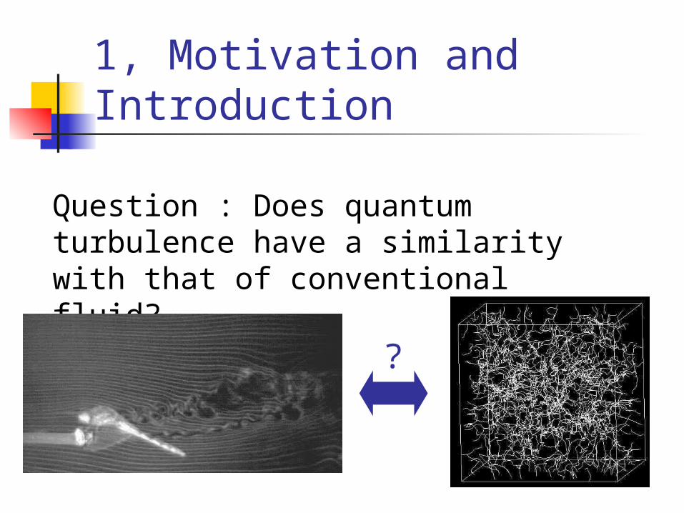
1, Motivation and Introduction
Question : Does quantum turbulence have a similarity with that of conventional fluid?
?

Why is This Important?
Quantum turbulence with quantized Quantum turbulence with quantized vortices can be an ideal prototype of vortices can be an ideal prototype of
turbulence!turbulence!
Quantum turbulence has the similarity with classical turbulence
Turbulence and Vortices : Kolmogorov Law of Classical Turbulence
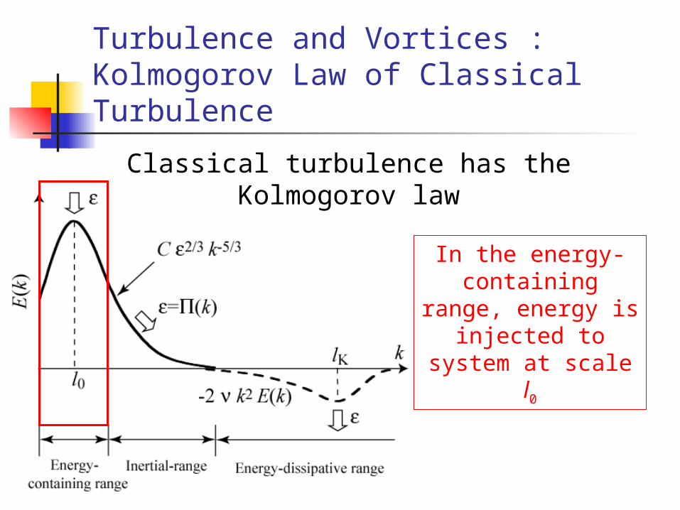
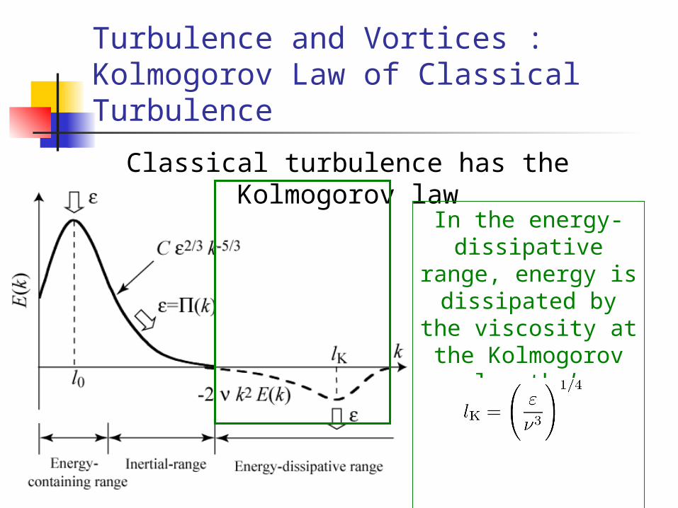
Classical turbulence has the Kolmogorov law
In the energy-containing range, energy is injected to system at scale
l0
Turbulence and Vortices : Kolmogorov Law of Classical Turbulence
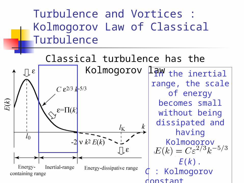
Classical turbulence has the Kolmogorov law In the inertial
range, the scale of energy becomes
small without being dissipated
and having Kolmogorov
energy spectrum E(k).
C : Kolmogorov constant
Turbulence and Vortices : Kolmogorov Law of Classical Turbulence
Classical turbulence has the Kolmogorov law
In the energy-dissipative range,
energy is dissipated by the viscosity at the
Kolmogorov length lK

Turbulence and Vortices : Kolmogorov Law of Classical Turbulence
Classical turbulence has the Kolmogorov law
: energy injection rate
: energy transportation rate
(k) : energy flux from large to small k
: energy dissipation rate

Turbulence and Vortices : Richardson Cascade
Kolmogorov law is believed to be sustained by the self-similar Richardson cascade of eddies.
Large eddies are nucleated
Eddies are broken up to smaller ones
Small eddies are dissipated

Difficulty of Studying Classical Turbulence
Vorticity = rot v takes continuous value. Circulation = ∳ v ・ ds takes arbitrary value for
arbitrary path. Eddies are nucleated and annihilated by the
viscosity. There is no global way to identify eddies.
Classical eddies are Classical eddies are indefinite!indefinite!
Quantized Vortex Is Definite Topological Defect
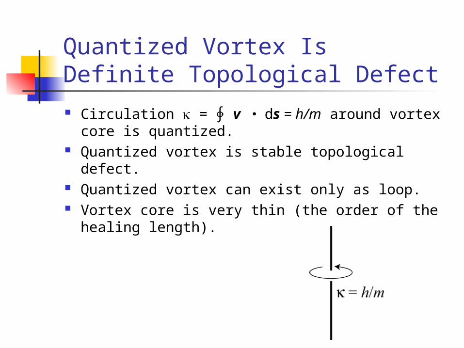
Circulation = ∳ v ・ ds = h/m around vortex core is quantized.
Quantized vortex is stable topological defect. Quantized vortex can exist only as loop. Vortex core is very thin (the order of the
healing length).

Quantum Turbulence Is an Ideal Prototype of Turbulence
Quantum turbulence can give the real Quantum turbulence can give the real Richardson cascade of definite Richardson cascade of definite topological defects and clarify the topological defects and clarify the statistics of turbulence. statistics of turbulence.
We study the We study the statistics of statistics of quantum turbulence quantum turbulence theoretically.theoretically.

Experimental Study of Turbulent State of Superfluid 4He
J. Maurer and P. Tabeling, Europhys. Lett. 43 (1), 29 (1998)
Two counter rotating disks
Temperature in experiment : T > 1.4 K
It is high to study a pure quantum turbulence.
Kolmogorov Law of Superfluid Turbulence
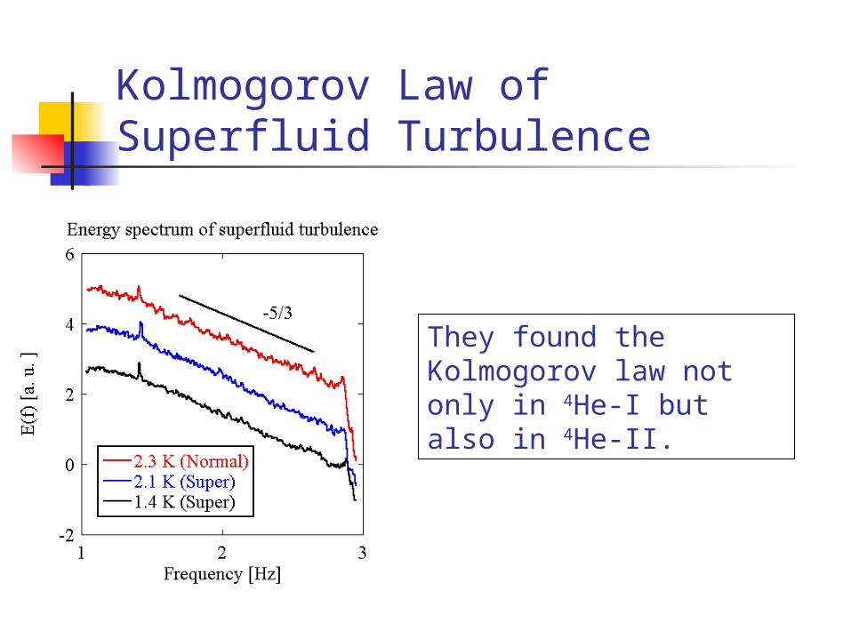
They found the Kolmogorov law not only in 4He-I but also in 4He-II.
Kolmogorov Law of Superfluid Turbulence
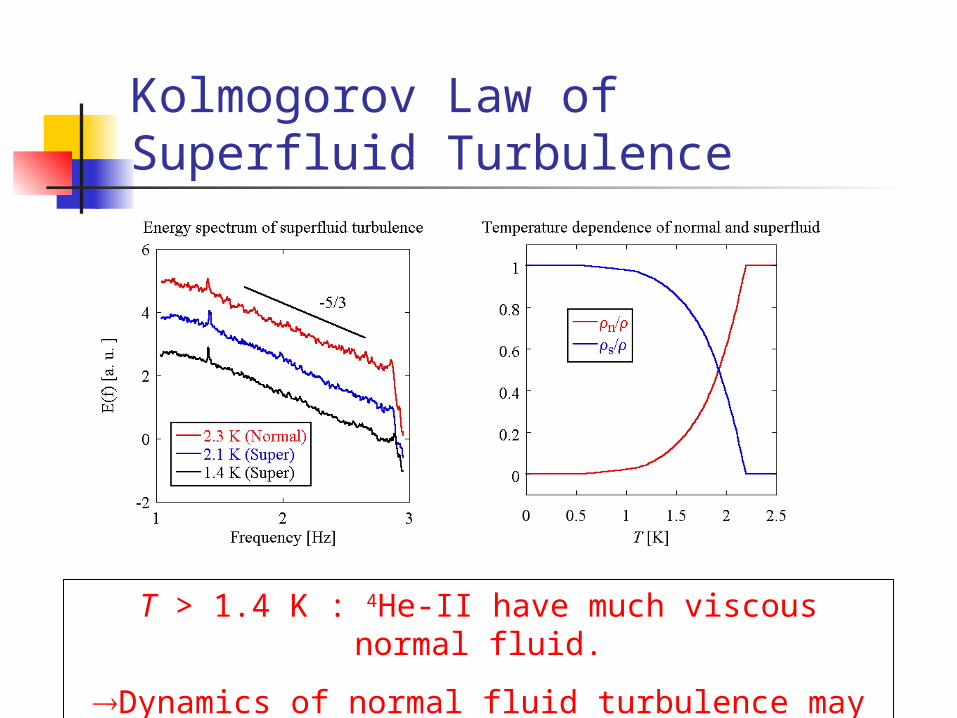
T > 1.4 K : 4He-II have much viscous normal fluid.
Dynamics of normal fluid turbulence may be dominant.

Motivation of This Work We study quantum turbulence at the
zero temperature by numerically solving the Gross-Pitaevskii equation.
By introducing a small-scale dissipation, we create pure quantum turbulence not affected by compressible short-wavelength excitations.
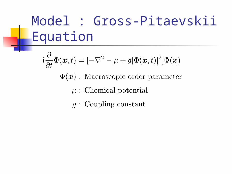
Model : Gross-Pitaevskii Equation

Model : Gross-Pitaevskii Equation
Quantized vortex
We numerically investigate We numerically investigate GP turbulence.GP turbulence.

Introducing a dissipation term
To remove the compressible short-wavelength excitations, we introduce a
small-scale dissipation term into GP equationFourier transformed GP equation
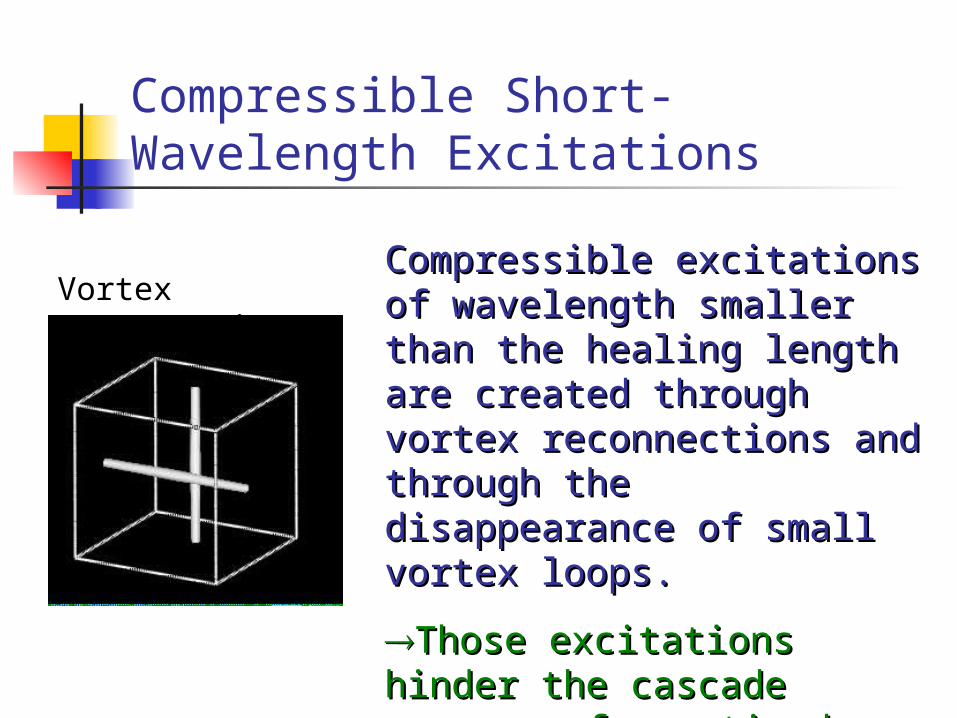
Compressible Short-Wavelength Excitations
Vortex reconnection
Compressible excitations of Compressible excitations of wavelength smaller than the wavelength smaller than the healing length are created healing length are created through vortex through vortex reconnections and through reconnections and through the disappearance of small the disappearance of small vortex loops.vortex loops.
Those excitations hinder Those excitations hinder the cascade process of the cascade process of quantized vortices!quantized vortices!

Without dissipating compressible excitations⋯
C. Nore, M. Abid, and M. E. Brachet, Phys. Rev. Lett. 78, 3896 (1997)
t = 2 t = 4
t = 6 t = 8
t = 12t = 10
Numerical simulation of GP turbulence
The incompressible kinetic energy changes to compressible kinetic energy while conserving the total energy
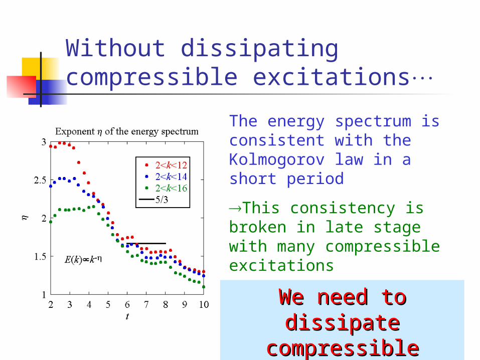
Without dissipating compressible excitations⋯
The energy spectrum is consistent with the Kolmogorov law in a short period
This consistency is broken in late stage with many compressible excitations
We need to dissipate We need to dissipate compressible compressible excitationsexcitations
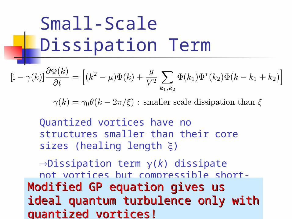
Small-Scale Dissipation Term
Quantized vortices have no structures smaller than their core sizes (healing length )
Dissipation term (k) dissipate not vortices but compressible short-wavelength excitationsModified GP equation gives us ideal Modified GP equation gives us ideal
quantum turbulence only with quantized quantum turbulence only with quantized vortices!vortices!

Simulation of Quantum Turbulence
1. Decaying turbulence starting from the random phase with no energy injection
2. Steady turbulence with energy injection
We numerically studied
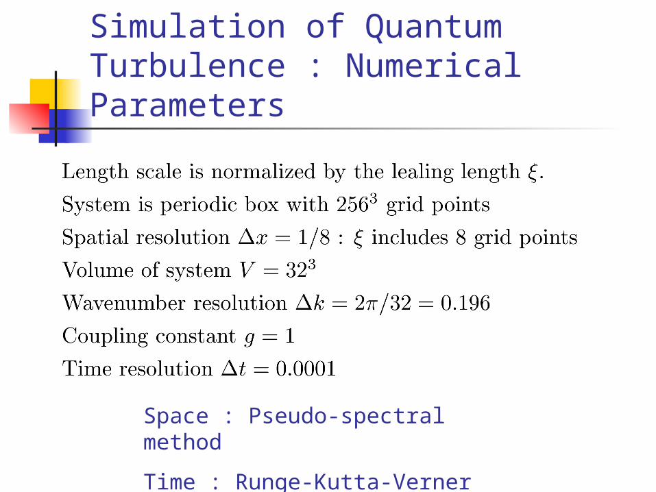
Simulation of Quantum Turbulence : Numerical Parameters
Space : Pseudo-spectral method
Time : Runge-Kutta-Verner method
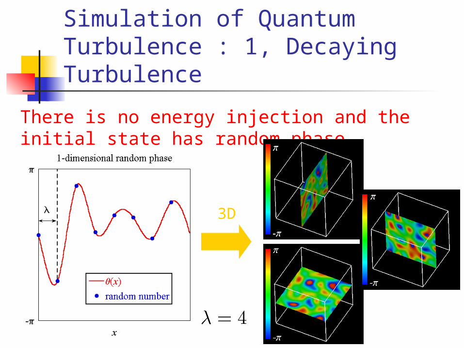
Simulation of Quantum Turbulence : 1, Decaying Turbulence
There is no energy injection and the initial state has random phase.
3D
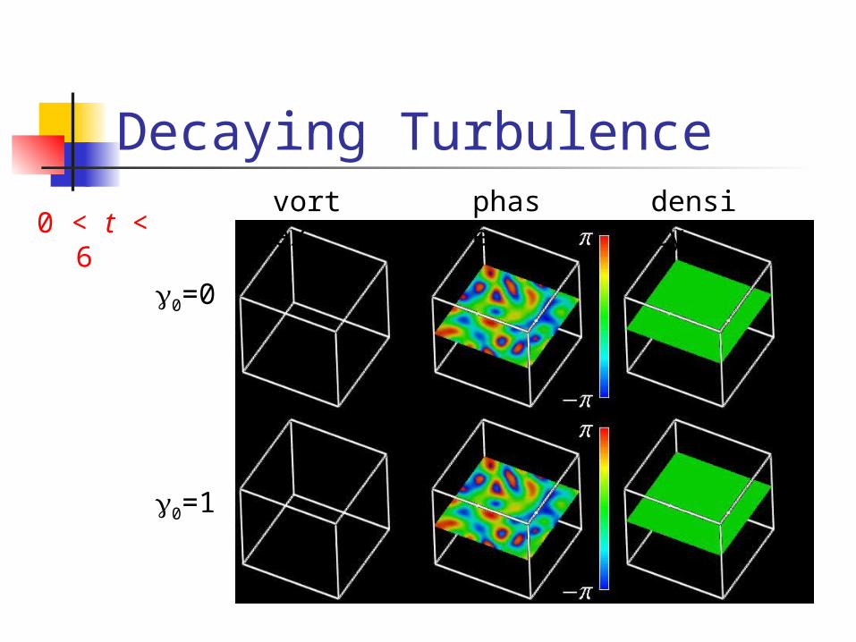
Decaying Turbulence
0 < t < 6
0=0
0=1
vortex
phase
density
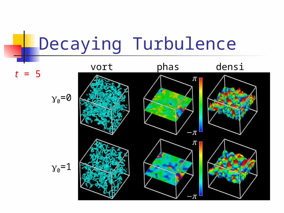
Decaying Turbulence
t = 5
0=0
0=1
vortex
phase
density

Decaying Turbulence
t = 5
0=0
0=1
density
Small structures in 0 = 0 are dissipated in 0 = 1
Dissipation term dissipates only short-wavelength excitations.
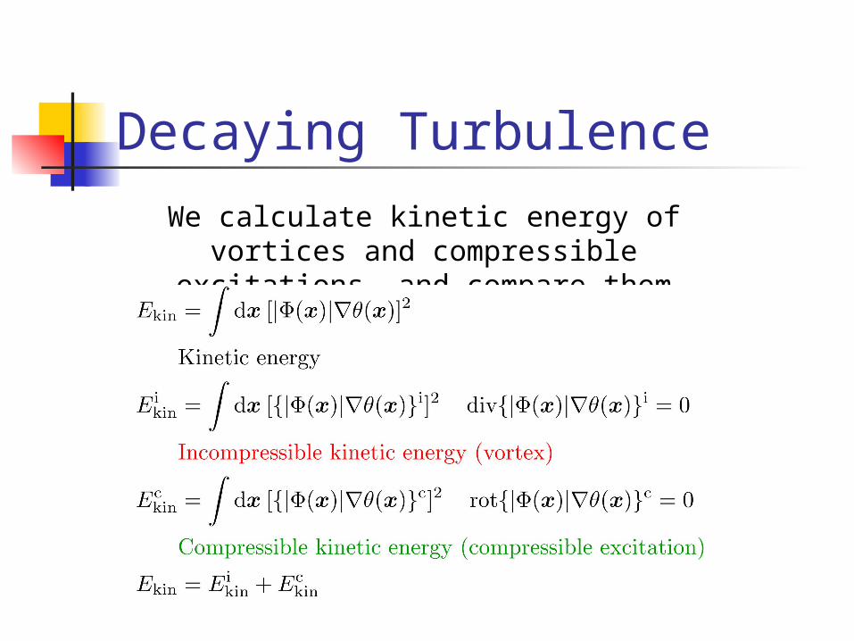
Decaying Turbulence
We calculate kinetic energy of vortices and compressible excitations, and compare them

Decaying Turbulence
0 = 0 : Energy of compressible excitations Ekinc is
dominant
0 = 1 : Energy of vortices Ekini is dominant
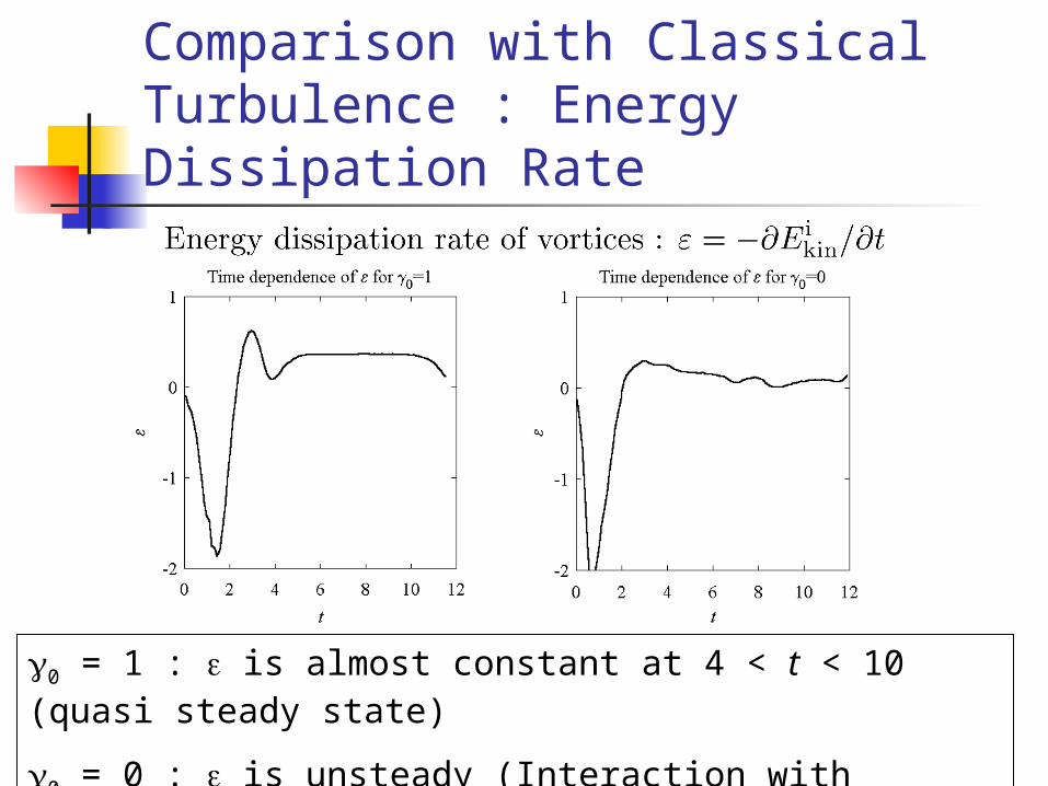
Comparison with Classical Turbulence : Energy Dissipation Rate
0 = 1 : is almost constant at 4 < t < 10 (quasi steady state)
0 = 0 : is unsteady (Interaction with compressible excitations)

Comparison with Classical Turbulence : Energy Spectrum
0 = 1 : = -5/3 at 4 < t < 10
0 = 0 : = -5/3 at 4 < t < 7
Straight line fitting at k < k < 2/
: Non-dissipating range

Comparison with Classical Turbulence : Energy Spectrum
By removing By removing compressible compressible excitations, quantum excitations, quantum turbulence show the turbulence show the similarity with similarity with classical turbulenceclassical turbulence

Simulation of Quantum Turbulence : 2, Steady Turbulence
Steady turbulence with the energy injection enables us to study detailed statistics of quantum turbulence.

Energy Injection as Moving Random Potential
X0 : characteristic scale of the moving random potential
Vortices of radius X0 are nucleated
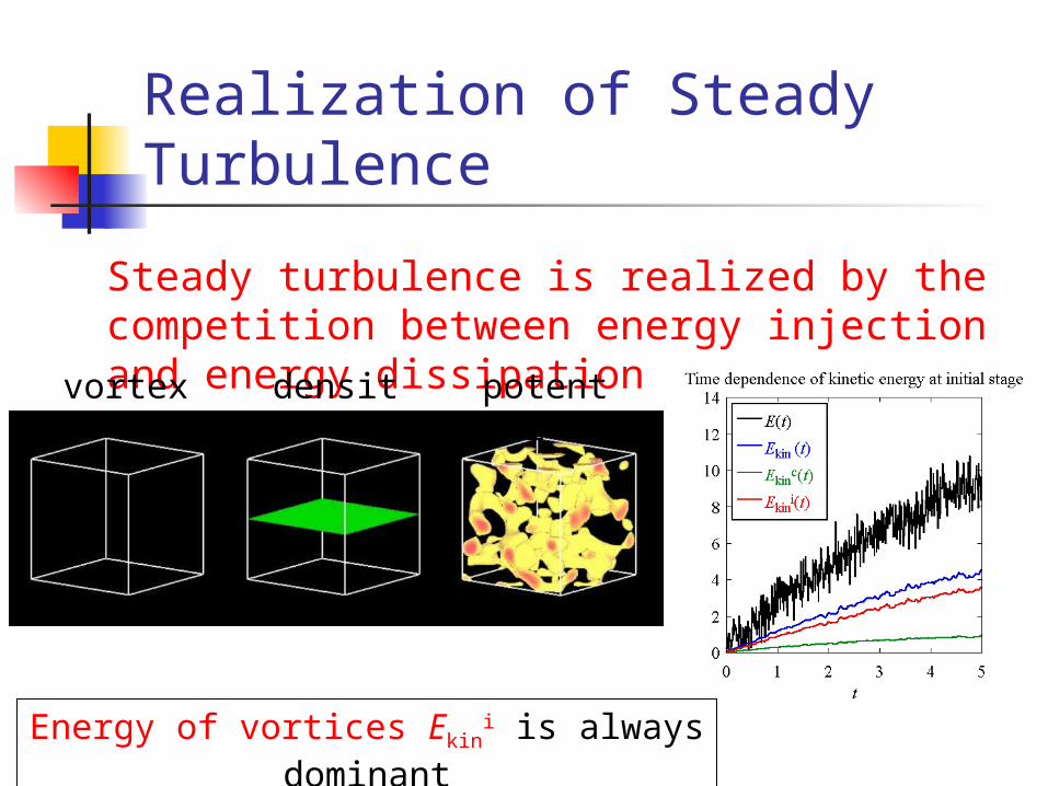
Realization of Steady Turbulence
Steady turbulence is realized by the competition between energy injection and energy dissipationvortex densit
ypotential
Energy of vortices Ekini is always
dominant
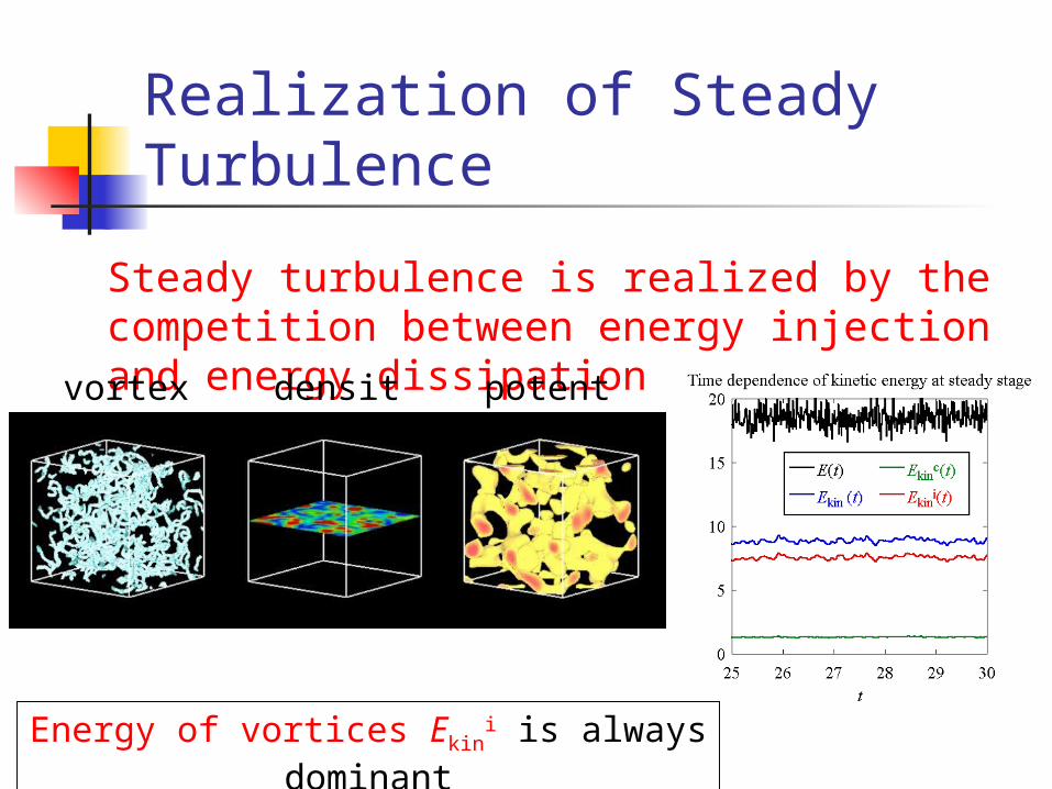
Realization of Steady Turbulence
Steady turbulence is realized by the competition between energy injection and energy dissipationvortex densit
ypotential
Energy of vortices Ekini is always
dominant

Flow of Kinetic Energy in Steady Turbulence
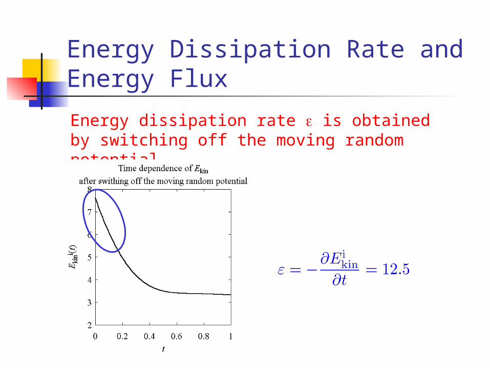
Energy Dissipation Rate and Energy Flux
Energy dissipation rate is obtained by switching off the moving random potential

Energy Dissipation Rate and Energy Flux
Energy flux (k) is obtained by the energy budget equation from the GP equation.
1. (k) is almost constant in the inertial range
2. (k) in the inertial range is consistent with the energy dissipation rate

Flow of Kinetic Energy in Steady Turbulence
Our picture of energy flow is Our picture of energy flow is correct!correct!
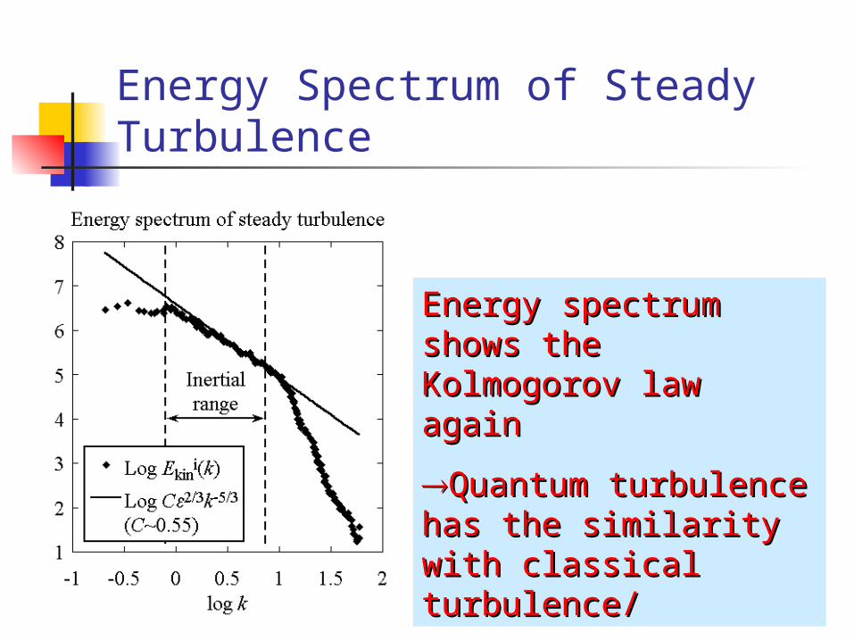
Energy Spectrum of Steady Turbulence
Energy spectrum Energy spectrum shows the Kolmogorov shows the Kolmogorov law againlaw again
Quantum turbulence Quantum turbulence has the similarity with has the similarity with classical turbulence/classical turbulence/
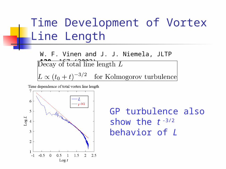
Time Development of Vortex Line Length
W. F. Vinen and J. J. Niemela, JLTP 128, 167 (2002)
GP turbulence also show the t -3/2 behavior of L

Comparison with Energy Spectrum
Initial stage
Energy spectrum is consistent with the Kolmogorov law

Comparison with Energy Spectrum
Middle stage
Consistency breaks down from large k (vortex mean free path)
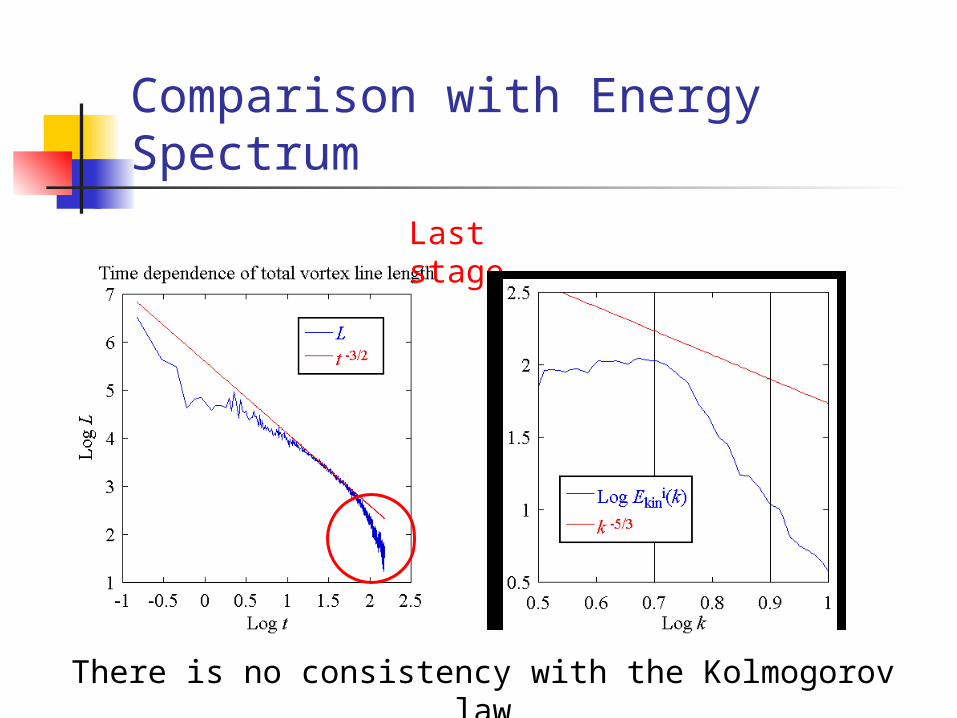
Comparison with Energy Spectrum
Last stage
There is no consistency with the Kolmogorov law

Dependence on Energy Injection
V0 = 50 (Strong Injection)
Kolmogorov law is clear
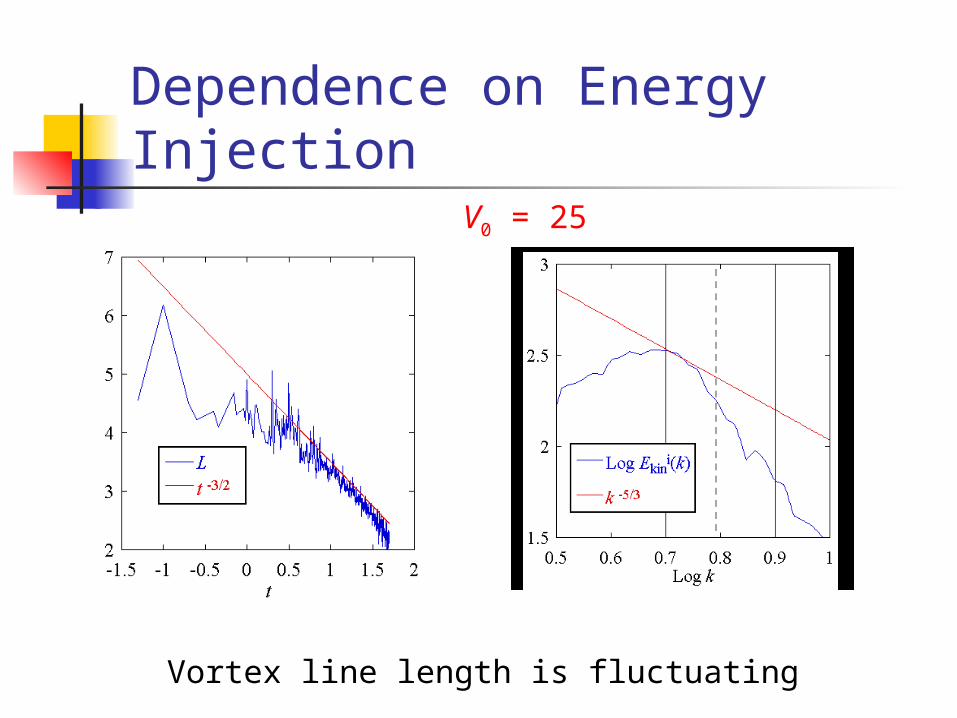
Dependence on Energy Injection
V0 = 25
Vortex line length is fluctuating

Dependence on Energy Injection
V0 = 10 (Weak Injection)
There is no Kolmogorov law
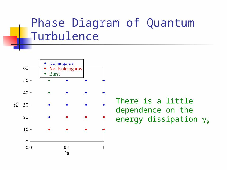
Phase Diagram of Quantum Turbulence
There is a little dependence on the energy dissipation 0

Application of Quantum Turbulence : Two-Component Quantum Turbulence
Two-component GP equation
gg1212 may be the important parameter may be the important parameter for the consistency with the for the consistency with the Kolmogorov law !Kolmogorov law !

Phase Diagram of Vortex Lattice
Triangular
Square
Sheet
g12/g
/1
0
K.K, M.Tsubota, and M.Ueda
g12 /g 1
K. Kasamatsu, M. Tsubota and M. Ueda, PRL 91, 150406 (2003)
Double Core

Two-Component Quantum Turbulence
g12
g12 = g
Kolmogorov law
???Kolmogorov law begins to break?
Self-organization of turbulence
Inter-component coupling may suppress the Richardson cascade and make another order of turbulence.
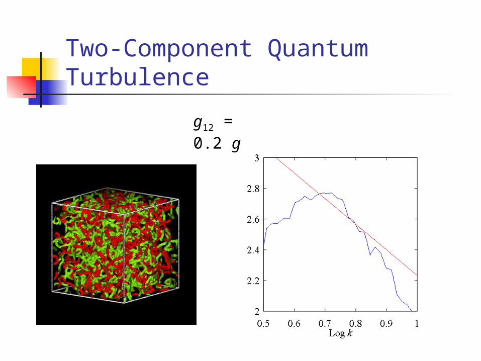
Two-Component Quantum Turbulence
g12 = 0.2 g

Summary By using modified GP equation
with the small scale dissipation term, we find the Kolmogorov law in quantum turbulence which means the similarity between quantum and classical turbulence.
Future works : Two-component quantum turbulence.


