70
Dynamics of Consumer Demand for New Durable Goods Gautam Gowrisankaran Marc Rysman University of Arizona, HEC Montreal, and NBER Boston University December 15, 2012

Dynamics of Consumer Demand for NewDurable Goods
Gautam Gowrisankaran Marc Rysman
University of Arizona, HEC Montreal, and NBER
Boston University
December 15, 2012
Introduction
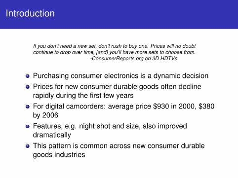
If you don’t need a new set, don’t rush to buy one. Prices will no doubtcontinue to drop over time, [and] you’ll have more sets to choose from.
-ConsumerReports.org on 3D HDTVs
Purchasing consumer electronics is a dynamic decisionPrices for new consumer durable goods often declinerapidly during the first few yearsFor digital camcorders: average price $930 in 2000, $380by 2006Features, e.g. night shot and size, also improveddramaticallyThis pattern is common across new consumer durablegoods industries

Why do dynamics matter?
A dynamic model is necessary to capture fact thatconsumers choose what to buy and when to buyRapidly evolving nature of industry suggests importance ofmodeling dynamicsRational consumer in 2000 would likely have expectedprice to drop and quality to rise

Idea of study
This paper specifies and estimates a structural dynamicmodel of consumer preferences for new durable goodsWe estimate the model using data on digital camcordersWe use the model to:
1 understand the importance of dynamics in consumerpreferences
2 evaluate dynamic price elasticities3 calculate a cost-of-living-index (COLI) for camcorders
Methods of inference are also potentially applicable toother industries and questions

Why estimate COLIs for new goods industries?
Concept is compensating variationsNecessary for government transfer programs and tounderstand contribution of innovation to the economyWell-known “new goods” problem (Pakes, 2003)There is also the “new buyer” problem (Aizcorbe, 2005)More generally
Consumers may wait to buy a digital camcorder until pricesdrop or features improveBut, high value consumers will buy early and then be out ofthe market until features improveThe two effects work in opposite directions
Suggests that estimation of a dynamic model is necessaryto sort out different effects

Features of model
Our model allows for product differentiation, persistentconsumer heterogeneity and repeat purchases over timeBerry, Levinsohn & Pakes (1995) [BLP] have shown theimportance of incorporating consumer heterogeneityMuch of our model is essentially the same as BLP
1 Consumers make a discrete choice over available models2 Multinomial logit utility with unobserved characteristic and
random coefficients3 Designed for model-level data but can also use
consumer-level data when available4 Allows for endogeneity of prices5 Evolution of models not chosen endogenously, e.g. with
respect to unobserved characteristics
Dynamics of our model
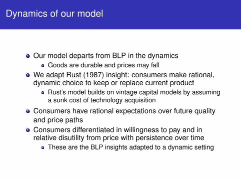
Our model departs from BLP in the dynamicsGoods are durable and prices may fall
We adapt Rust (1987) insight: consumers make rational,dynamic choice to keep or replace current product
Rust’s model builds on vintage capital models by assuminga sunk cost of technology acquisition
Consumers have rational expectations over future qualityand price pathsConsumers differentiated in willingness to pay and inrelative disutility from price with persistence over time
These are the BLP insights adapted to a dynamic setting

Biases from not modeling dynamics
Dynamics transforms consumption problem into aninvestment problemFirms will invest in capital if service flow is greater thanrental cost:
Rental cost of capital is difference in present-value pricesFor static models: increase in sales as prices dropFor dynamic models: increase only when drop ends
Static estimation applied to durable goods purchaseresults in measurements error
Price coefficients biased towards zero
Heterogeneous agents imply that population response torising quality is smaller than average individual responseMay be hard to rationalize cross-sectional and dynamicsubstitution patterns with static model

Relation to literature
Other recent papers have also been developing dynamicmodels of demand
Our paper builds on work by Melnikov (2012) among others
Ours is the first paper to use BLP-style model of per-perioddemand and to allow for repeat purchasesSeveral new papers use and extend our methods toexamine related I.O. and antitrust questions
Shcherbakov (2009), Ho (2011) and Nosal (2012) estimateswitching costsSchiraldi (2011) examines dynamics of automobile marketLee (2012) examines video-game platform competitionZhao (2008) estimates digital camera market
We provide code and assistance to implement ouralgorithm

Model
Model starts at time t = 0 with introduction of new segmentUnit of observation is a monthFuture discounted at rate β by consumers and firmsOur model nests insights of Rust-style optimal stoppingmodel inside BLP-style model
Our exposition first focuses on the single consumerUltimately, we model continuum of consumers
Forward-looking consumer can purchase durable good, orhold outside good (with flow utility 0)Durable good does not depreciate, but consumer can onlyobtain utility from one good at a time

Consumer preferences
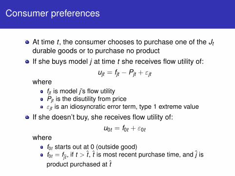
At time t , the consumer chooses to purchase one of the Jtdurable goods or to purchase no product
If she buys model j at time t she receives flow utility of:ujt = fjt − Pjt + εjt
wherefjt is model j ’s flow utilityPjt is the disutility from priceεjt is an idiosyncratic error term, type 1 extreme value
If she doesn’t buy, she receives flow utility of:u0t = f0t + ε0t
wheref0t starts out at 0 (outside good)f0t = fj t , if t > t , t is most recent purchase time, and j isproduct purchased at t

Consumer preferences
At time t , the consumer chooses to purchase one of the Jtdurable goods or to purchase no productIf she buys model j at time t she receives flow utility of:
ujt = fjt − Pjt + εjt
wherefjt is model j ’s flow utilityPjt is the disutility from priceεjt is an idiosyncratic error term, type 1 extreme value
If she doesn’t buy, she receives flow utility of:u0t = f0t + ε0t
wheref0t starts out at 0 (outside good)f0t = fj t , if t > t , t is most recent purchase time, and j isproduct purchased at t

Consumer expectations
At time t , consumer has Jt + 1 choices and maximizesexpected discounted utility of future utilityConsumer knows time all t information when making herdecisions but does not know future ~ε shocksFuture models vary due to entry, exit and price changesand the consumer may lack perfect informationLet Ωt denote number of models, model attributes andother factors that may influence future model attributesWe assume that Ωt evolves according to a Markovprocess, P (Ωt+1|Ωt )
State space is (~εt , f0t ,Ωt )

Dynamics of consumer preferences
Bellman equation prior to realization of ~ε:
V (f0,Ω) =∫
max
Value of keeping existing model︷ ︸︸ ︷f0 + βE
[V(f0,Ω′)∣∣Ω
]+ ε0,
maxj=1,...,Jfj − Pj + βE[V(fj ,Ω′)∣∣Ω
]+ εj︸ ︷︷ ︸
Value of upgrading to j
g~ε(~ε)
where “E” is expectation and “ ′ ” is next periodInterpretation:
First line: keep existing model, get f0 going forwardSecond line: upgrade, get fj going forward
Problem: dimension of Ω is huge
State space simplification
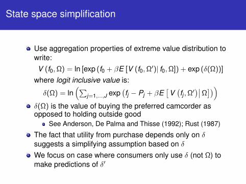
Use aggregation properties of extreme value distribution towrite:V (f0,Ω) = ln [exp (f0 + βE [V (f0,Ω′)| f0,Ω]) + exp (δ(Ω))]
where logit inclusive value is:
δ(Ω) = ln(∑
j=1,...,J exp(fj − Pj + βE
[V(fj ,Ω′)∣∣Ω
]))δ(Ω) is the value of buying the preferred camcorder asopposed to holding outside good
See Anderson, De Palma and Thisse (1992); Rust (1987)
The fact that utility from purchase depends only on δsuggests a simplifying assumption based on δWe focus on case where consumers only use δ (not Ω) tomake predictions of δ′
Inclusive value sufficiency
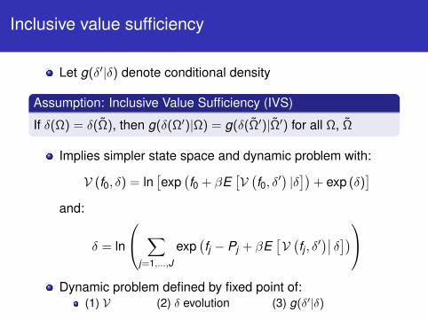
Let g(δ′|δ) denote conditional density
Assumption: Inclusive Value Sufficiency (IVS)
If δ(Ω) = δ(Ω), then g(δ(Ω′)|Ω) = g(δ(Ω′)|Ω′) for all Ω, Ω
Implies simpler state space and dynamic problem with:
V (f0, δ) = ln[exp
(f0 + βE
[V(f0, δ′) |δ])+ exp (δ)
]and:
δ = ln
∑j=1,...,J
exp(fj − Pj + βE
[V(fj , δ′)∣∣ δ])
Dynamic problem defined by fixed point of:
(1) V (2) δ evolution (3) g(δ′|δ)
Inclusive value sufficiency
Let g(δ′|δ) denote conditional density
Assumption: Inclusive Value Sufficiency (IVS)
If δ(Ω) = δ(Ω), then g(δ(Ω′)|Ω) = g(δ(Ω′)|Ω′) for all Ω, Ω
Implies simpler state space and dynamic problem with:
V (f0, δ) = ln[exp
(f0 + βE
[V(f0, δ′) |δ])+ exp (δ)
]and:
δ = ln
∑j=1,...,J
exp(fj − Pj + βE
[V(fj , δ′)∣∣ δ])
Dynamic problem defined by fixed point of:
(1) V (2) δ evolution (3) g(δ′|δ)

Expectations of δ evolution
We assume rational expectationsOne option is perfect foresightWe believe that limited ability to predict future modelattributes is more realistic
For most specifications, we let perceptions about nextperiod’s δ be empirical density fitted to autoregressivespecification:
δt+1 = γ1 + γ2δt + νt+1
Similar – but not identical – assumptions as in Melnikov(2001) and Hendel and Nevo (2006)
Due to repeat purchases, we first need to define δ as entirefuture utility stream, not flow utility
Role of δ and IVS assumption in numerical example
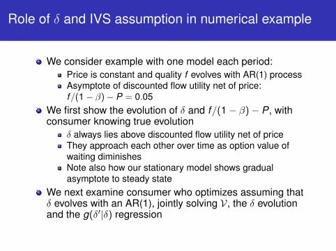
We consider example with one model each period:Price is constant and quality f evolves with AR(1) processAsymptote of discounted flow utility net of price:f/(1− β)− P = 0.05
We first show the evolution of δ and f/(1− β)− P, withconsumer knowing true evolution
δ always lies above discounted flow utility net of priceThey approach each other over time as option value ofwaiting diminishesNote also how our stationary model shows gradualasymptote to steady state
We next examine consumer who optimizes assuming thatδ evolves with an AR(1), jointly solving V, the δ evolutionand the g(δ′|δ) regression
Errors from approximation are small

Role of δ and IVS assumption in numerical example-1
0-8
-6-4
-20
0 20 40 60 80 100Time
Discounted flow util ity net of pr ice Delta

Role of δ and IVS assumption in numerical example
We consider example with one model each period:Price is constant and quality f evolves with AR(1) processAsymptote of discounted flow utility net of price:f/(1− β)− P = 0.05
We first show the evolution of δ and f/(1− β)− P, withconsumer knowing true evolution
δ always lies above discounted flow utility net of priceThey approach each other over time as option value ofwaiting diminishesNote also how our stationary model shows gradualasymptote to steady state
We next examine consumer who optimizes assuming thatδ evolves with an AR(1), jointly solving V, the δ evolutionand the g(δ′|δ) regression
Errors from approximation are small

Role of δ and IVS assumption in numerical example
0.0
1.0
2.0
3
0 20 40 60 80 100Time
Market share when consumer uses IVS data generating processMarket share when consumer knows true data generating process

Role of δ and IVS assumption in numerical example
We consider example with one model each period:Price is constant and quality f evolves with AR(1) processAsymptote of discounted flow utility net of price:f/(1− β)− P = 0.05
We first show the evolution of δ and f/(1− β)− P, withconsumer knowing true evolution
δ always lies above discounted flow utility net of priceThey approach each other over time as option value ofwaiting diminishesNote also how our stationary model shows gradualasymptote to steady state
We next examine consumer who optimizes assuming thatδ evolves with an AR(1), jointly solving V, the δ evolutionand the g(δ′|δ) regression
Errors from approximation are small
Empirical tests of IVS assumption
We also try:adding J as a stateAdding month effectsEmpirically testing the assumption
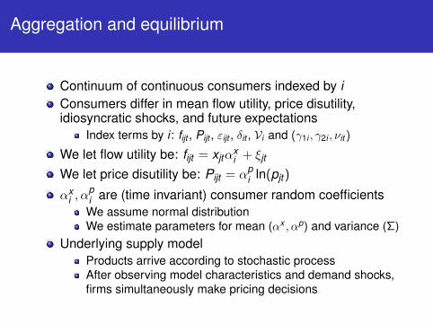
Aggregation and equilibrium
Continuum of continuous consumers indexed by iConsumers differ in mean flow utility, price disutility,idiosyncratic shocks, and future expectations
Index terms by i : fijt , Pijt , εijt , δit , Vi and (γ1i , γ2i , νit )
We let flow utility be: fijt = xjtαxi + ξjt
We let price disutility be: Pijt = αpi ln(pjt )
αxi , α
pi are (time invariant) consumer random coefficientsWe assume normal distributionWe estimate parameters for mean (αx , αp) and variance (Σ)
Underlying supply modelProducts arrive according to stochastic processAfter observing model characteristics and demand shocks,firms simultaneously make pricing decisions

Inference
Parameters are α, Σ and βDifficult to estimate discount factor, so we set β = .99 atlevel of month
Following BLP, we specify a GMM criterion function:
G (α,Σ) = z ′~ξ (α,Σ)
Actual criterion function also includes micro-moments as inPetrin (2002)We estimate parameters to satisfy:(
α, Σ)
= arg minα,Σ
G (α,Σ)′ WG (α,Σ)
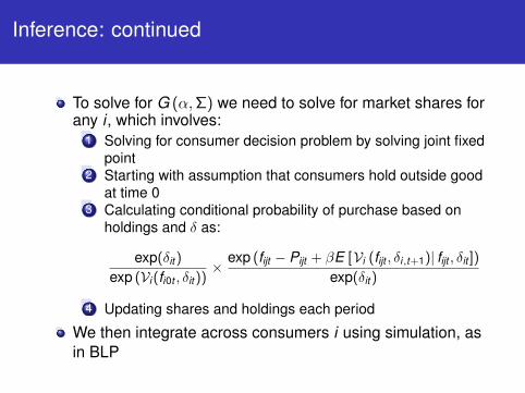
Inference: continued
To solve for G (α,Σ) we need to solve for market shares forany i , which involves:
1 Solving for consumer decision problem by solving joint fixedpoint
2 Starting with assumption that consumers hold outside goodat time 0
3 Calculating conditional probability of purchase based onholdings and δ as:
exp(δit )
exp (Vi (fi0t , δit ))×
exp (fijt − Pijt + βE [Vi (fijt , δi,t+1)| fijt , δit ])
exp(δit )
4 Updating shares and holdings each period
We then integrate across consumers i using simulation, asin BLP

Obtaining ξ from shares
Define mean flow utility as:
Fjt = xjtαx + ξjt , j = 1, . . . , Jt
Moment condition requires backing out ~ξ from observedshares:
sjt − sjt
(~F , αp,Σ
)We use:
F newjt = F new
jt + ψ ·(
ln(sjt )− ln(
sjt
(~F old , αp,Σ
))), ∀j , t
We solve for simultaneous fixed point of Fjt , Vi and δi ,updating g(δ′
i |δi) and conditional probability of purchaseAt fixed point, true shares equal predicted shares andconsumers are optimizing

Why is our method useful?
Alternative might be maximum likelihoodMaximum likelihood that accounted for endogeneity wouldhave to explicitly calculate dynamic firm problemInversion method allows us to estimate consumer modelwithout explicitly solving equilibriumComputationally much easier and needs (somewhat) lessassumptions

Instruments
We use all model characteristics as instrumentsUse also mean model characteristics within a firm at time tand overall at time tUse also count of number of models within a firm andoverall at time t

Identification
Our parameters all static consumer preference parametersThis is true even for the repeat purchase model because ofreasonably strong assumptions: digital camcorders don’twear out; there is no resale market for them; and only onedigital camcorder per household is usefulIdentification arguments similar to static discrete choiceliterature, e.g. Berry (1994), Petrin (2002)Variation in “nearby” models will identify price elasticitiesRandom coefficients identified by variation in choice sets;e.g. how do consumers substitute as choice set variesDynamics helps identification: random coefficients alsoidentified by endogenous differences in tastes over timeand substitution across time
Data
Aggregate data on prices, quantities andcharacteristics for digital camcordersPrices declining and quantities rising over timeBig issue is Christmas; we seasonally adjust data toaccount for ChristmasData from 2000 to 2006; features improving over timeSome specifications use household penetration data fromICR-CENTRIS

Data
56
78
910
Brands
2040
6080
100
Models
Jan00 Jan02 Jan04 Jan06
Models Brands
Data
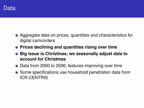
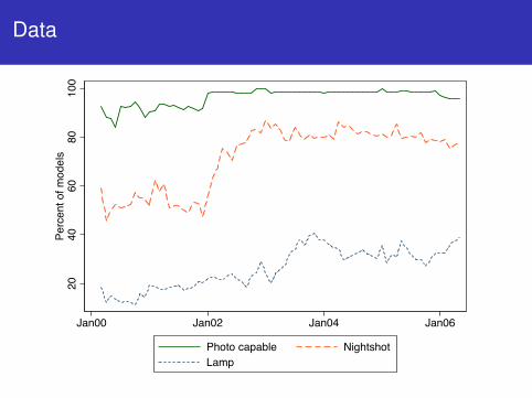
Aggregate data on prices, quantities and characteristics fordigital camcordersPrices declining and quantities rising over timeBig issue is Christmas; we seasonally adjust data toaccount for ChristmasData from 2000 to 2006; features improving over timeSome specifications use household penetration data fromICR-CENTRIS

Data
400
400
600
600
800
800
1000
1000
Price in Jan. 2000 dollars
Pric
e in
Jan
. 200
0 do
llars
0
0
200
200
400
400
600
600
Sales in thousands of units
Sale
s in
tho
usan
ds o
f un
its
Jan00
Jan00
Jan02
Jan02
Jan04
Jan04
Jan06
Jan06
Seasonally-adjusted sales
Seasonally-adjusted sales
Sales
Sales
Price
Price

Data
Aggregate data on prices, quantities and characteristics fordigital camcordersPrices declining and quantities rising over timeBig issue is Christmas; we seasonally adjust data toaccount for ChristmasData from 2000 to 2006; features improving over timeSome specifications use household penetration data fromICR-CENTRIS

Data
1015
2025
Size
(wid
th X
dep
th, i
n.)
.6.8
11.
2pi
xels
(milli
on)
Jan00 Jan02 Jan04 Jan06
Pixel count Size
Data
2040
6080
100
Perc
ent o
f mod
els
Jan00 Jan02 Jan04 Jan06
Photo capable NightshotLamp

Data
020
4060
8010
0Pe
rcen
t of m
odel
s
Jan00 Jan02 Jan04 Jan06month
Tape DVDFlash Hard drive
Data
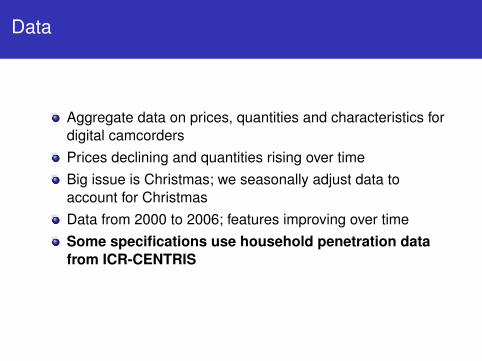
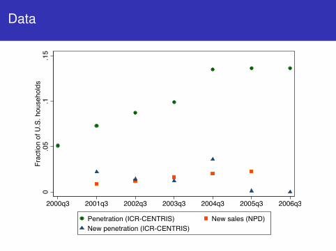
Aggregate data on prices, quantities and characteristics fordigital camcordersPrices declining and quantities rising over timeBig issue is Christmas; we seasonally adjust data toaccount for ChristmasData from 2000 to 2006; features improving over timeSome specifications use household penetration datafrom ICR-CENTRIS
Data
0.0
5.1
.15
Frac
tion
of U
.S. h
ouse
hold
s
2000q3 2001q3 2002q3 2003q3 2004q3 2005q3 2006q3
Penetration (ICR-CENTRIS) New sales (NPD)New penetration (ICR-CENTRIS)

Results and fit of the model
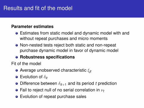
Parameter estimatesEstimates from static model and dynamic model withand without repeat purchases and micro momentsNon-nested tests reject both static and non-repeatpurchase dynamic model in favor of dynamic modelRobustness specifications
Fit of the modelAverage unobserved characteristic ξjt
Evolution of δit
Difference between δit+1 and its period t predictionFail to reject null of no serial correlation in νt
Evolution of repeat purchase sales

Results and fit of the model
ParameterBase dynamic
model
Dynamic model without repurchases
Static modelDynamic model with micro‐moment
(1) (2) (3) (4)
Mean coefficients (α)Constant ‐.092 (.029) * ‐.093 (7.24) ‐6.86 (358) ‐.367 (.065) *
Log price ‐3.30 (1.03) * ‐.543 (3.09) ‐.099 (148) ‐3.43 (.225) *
Log size ‐.007 (.001) * ‐.002 (.116) ‐.159 (.051) * ‐.021 (.003) *
Log pixel .010 (.003) * ‐.002 (.441) ‐.329 (.053) * .027 (.003) *
Log zoom .005 (.002) * .006 (.104) .608 (.075) * .018 (.004) *
Log LCD size .003 (.002) * .000 (.141) ‐.073 (.093) .004 (.005)
Media: DVD .033 (.006) * .004 (1.16) .074 (.332) .060 (.019) *
Media: tape .012 (.005) * ‐.005 (.683) ‐.667 (.318) * .015 (.018)
Media: HD .036 (.009) * ‐.002 (1.55) ‐.647 (.420) .057 (.022) *
Lamp .005 (.002) * ‐.001 (.229) ‐.219 (.061) * .002 (.003)
Night shot .003 (.001) * .004 (.074) .430 (.060) * .015 (.004) *
Photo capable ‐.007 (.002) * ‐.002 (.143) ‐.171 (.173) ‐.010 (.006)
Standard deviation coefficients (Σ1/2)Constant .079 (.021) * .038 (1.06) .001 (1147) .087 (.038) *
Log price .345 (.115) * .001 (1.94) ‐.001 (427) .820 (.084) *
Standard errors in parentheses; statistical significance at 5% level indicated with *. All models include brand dummies, with Sony excluded. There are 4436 observations.
Results and fit of the model
Parameter estimatesEstimates from static model and dynamic model with andwithout repeat purchases and micro momentsNon-nested tests reject both static and non-repeatpurchase dynamic model in favor of dynamic modelRobustness specifications
Fit of the modelAverage unobserved characteristic ξjt
Evolution of δit
Difference between δit+1 and its period t predictionFail to reject null of no serial correlation in νt
Evolution of repeat purchase sales
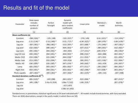
Results and fit of the model
Parameter
State space includes number of products
Perfect foresight
Dynamic model with extra random coefficients
Linear priceMelnikov's model
Month dummies
(1) (2) (3) (4) (5) (6)Mean coefficients (α)
Constant ‐.098 (.026) * ‐.129 (.108) ‐.103 (.037) * ‐.170 (.149) ‐6.61 (.815) * ‐.114 (.024) *
Log price ‐3.31 (1.04) * ‐2.53 (.940) * ‐3.01 (.717) * ‐6.94 (.822) * ‐.189 (.079) * ‐3.06 (.678) *
Log size ‐.007 (.001) * ‐.006 (.001) * ‐.015 (.007) * .057 (.008) * ‐.175 (.049) * ‐.007 (.001) *
Log pixel .010 (.003) * .008 (.001) * .009 (.002) * .037 (.012) * ‐.288 (.053) * .010 (.002) *
Log zoom .005 (.002) * .004 (.002) * .004 (.002) ‐.117 (.012) * .609 (.074) * .005 (.002)*
Log LCD size .004 (.002) * .004 (.001) * .004 (.002) * .098 (.010) * ‐.064 (.088) .003 (.001) *
Media: DVD .033 (.006) * .025 (.004) * .044 (.018) * .211 (.053) * .147 (.332) .031 (.005) *
Media: tape .013 (.005) * .010 (.004) * .024 (.016) .200 (.051) * ‐.632 (.318) * .012 (.004) *
Media: HD .036 (.009) * .026 (.005) * .047 (.019) * .349 (.063) * ‐.545 (.419) .034 (.007) *
Lamp .005 (.002) * .003 (.001) * .005 (.002) * .077 (.011) * ‐.200 (.058) * .004 (.001) *
Night shot .003 (.001) * .004 (.001) * .003 (.001) * ‐.062 (.008) * .427 (.058) * .003 (.001) *
Photo capable ‐.007 (.002) * ‐.005 (.002) * ‐.007 (.002) * ‐.061 (.019) * ‐.189 (.142) ‐.007 (.008)Standard deviation coefficients (Σ1/2)
Constant .085 (.019) * .130 (.098) .081 (.025) * .022 (.004) * .087 (.013) *
Log price .349 (.108) * 2.41e‐9 (.919) 1.06e‐7 (.522) 1.68 (.319) * .287 (.078) *
Log size ‐.011 (.007)
Log pixel 1.58e‐10 (.002)
Standard errors in parentheses; statistical significance at 5% level indicated with *. All models include brand dummies, with Sony excluded. There are 4436 observations, except in the yearly model, in which there are 505.

Results and fit of the model
Parameter estimatesEstimates from static model and dynamic model with andwithout repeat purchases and micro momentsNon-nested tests reject both static and non-repeatpurchase dynamic model in favor of dynamic modelRobustness specifications
Fit of the modelAverage unobserved characteristic ξjt
Evolution of δit
Difference between δit+1 and its period t predictionFail to reject null of no serial correlation in νt
Evolution of repeat purchase sales
Results and fit of the model-.0
1-.0
050
.005
.01
Jan00 Jan02 Jan04 Jan06
Mean xi Zero base

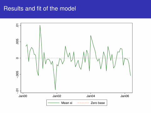
Results and fit of the model
Parameter estimatesEstimates from static model and dynamic model with andwithout repeat purchases and micro momentsNon-nested tests reject both static and non-repeatpurchase dynamic model in favor of dynamic modelRobustness specifications
Fit of the modelAverage unobserved characteristic ξjt
Evolution of δit
Difference between δit+1 and its period t predictionFail to reject null of no serial correlation in νt
Evolution of repeat purchase sales

Results and fit of the model
3.4
3.6
3.8
4D
iffer
ence
bet
wee
n 80
-80
and
20-8
0
-25
-20
-15
-10
-50
delta
_it
Jan00 Jan02 Jan04 Jan06
Coeffs in 80th percentile Coeffs in 20th percentilePrice in 20th, const in 80th Difference between 80-80 and 20-80

Results and fit of the model
Parameter estimatesEstimates from static model and dynamic model with andwithout repeat purchases and micro momentsNon-nested tests reject both static and non-repeatpurchase dynamic model in favor of dynamic modelRobustness specifications
Fit of the modelAverage unobserved characteristic ξjt
Evolution of δit
Difference between δit+1 and its period t predictionFail to reject null of no serial correlation in νt
Evolution of repeat purchase sales

Results and fit of the model-.5
0.5
1
Jan00 Jan02 Jan04 Jan06
Mean consumer prediction error Zero base
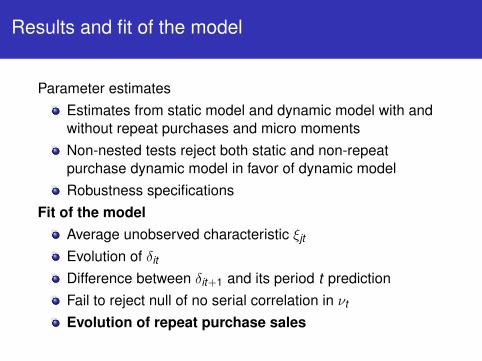
Results and fit of the model
Parameter estimatesEstimates from static model and dynamic model with andwithout repeat purchases and micro momentsNon-nested tests reject both static and non-repeatpurchase dynamic model in favor of dynamic modelRobustness specifications
Fit of the modelAverage unobserved characteristic ξjt
Evolution of δit
Difference between δit+1 and its period t predictionFail to reject null of no serial correlation in νt
Evolution of repeat purchase sales

Results and fit of the model
0.1
.2.3
Frac
tion
of s
ales
from
repe
at p
urch
aser
s
Jan00 Jan02 Jan04 Jan06
Base model Model with additional moment
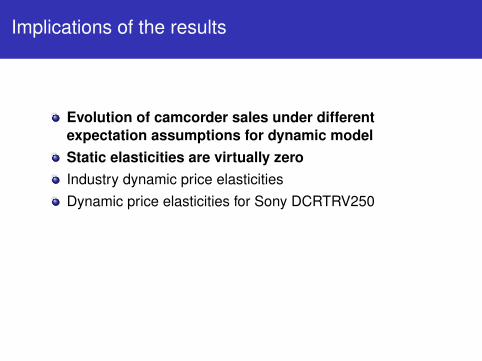
Implications of the results
Evolution of camcorder sales under differentexpectation assumptions for dynamic modelStatic elasticities are virtually zeroIndustry dynamic price elasticitiesDynamic price elasticities for Sony DCRTRV250

Implications of the results
0.0
02.0
04.0
06Fr
actio
n of
hou
seho
lds
purc
hasi
ng
Jan00 Jan02 Jan04 Jan06
Share Share if cons. always inShare if cons. assume same future

Implications of the results
Evolution of camcorder sales under different expectationassumptions for dynamic modelStatic elasticities are virtually zeroIndustry dynamic price elasticitiesDynamic price elasticities for Sony DCRTRV250

Implications of the results
-2.5
-2-1
.5-1
-.50
Perc
ent q
uant
ity c
hang
e fro
m b
asel
ine
-5 0 5 10 15Months after price change
Permanent price change Temp. price change

Implications of the results
Evolution of camcorder sales under different expectationassumptions for dynamic modelStatic elasticities are virtually zeroIndustry dynamic price elasticitiesDynamic price elasticities for Sony DCRTRV250

Implications of the results
-2.5
-2-1
.5-1
-.50
Perc
ent q
uant
ity c
hang
e fro
m b
asel
ine
-5 0 5 10 15Months after price change
Permanent price change Temp. price change
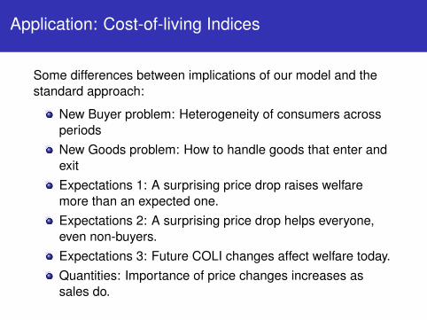
Application: Cost-of-living Indices
Some differences between implications of our model and thestandard approach:
New Buyer problem: Heterogeneity of consumers acrossperiodsNew Goods problem: How to handle goods that enter andexitExpectations 1: A surprising price drop raises welfaremore than an expected one.Expectations 2: A surprising price drop helps everyone,even non-buyers.Expectations 3: Future COLI changes affect welfare today.Quantities: Importance of price changes increases assales do.

Our approach
Imagine the set of state-contingent taxes that keepaverage expected welfare constantEquivalently, the set of state-contingent taxes that keepsaverage flow utility constant
Assume that consumers dynamically optimizeMeans we don’t have to average over all possiblesequences of outcomes to compute price index
Compute tax for sequence of realized statesAssume price is paid in an infinite stream of constantpayments

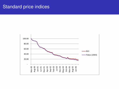
Our implementation of the BLS approach
Laspeyres price index:
It+1
It=
∑Jtj=1 sjtpj,t+1∑Jt
j=1 sjtpjt
Need assumptions on prices for models that exit
BLS: impute price from average price dropPakes (2003): predict price from a regression oncharacteristics
Good 0 is outside option and has a price that doesn’tchangeMultiply price index by average price at t = 0 ($969) to getequivalent to our tax
Standard price indices
100.00
60.00
80.00
BLS
20 00
40.00 BLS
Pakes (2003)
‐
20.00
00 00 01 01 01 02 02 03 03 03 04 04 05 05 06
Mar‐0
Aug
‐0
Jan‐0
Jun‐0
Nov‐0
Apr‐0
Sep‐0
Feb‐0
Jul‐0
Dec‐0
May‐0
Oct‐0
Mar‐0
Aug
‐0
Jan‐0

Changes in cost-of-living
0.5
11.
52
Tax
in y
ear 2
000
dolla
rs
Jan00 Jan02 Jan04 Jan06
BLS COLI COLI from dynamic estimatesPakes COLI
Results from COLI exercise
BLS computes the income change necessary to allow aHH to buy a constant quality camcorder in each periodWe compute the income change necessary to hold utilityconstant
These diverge because as households accumulate thegood, they value a new one lessLevel differences are somewhat arbitrary, but shapedifferences are importantBLS price index continues to drop because prices do,whereas ours recognizes that later buyers are lower value

Results from COLI exercise
BLS computes the income change necessary to allow aHH to buy a constant quality camcorder in each periodWe compute the income change necessary to hold utilityconstantThese diverge because as households accumulate thegood, they value a new one less
Level differences are somewhat arbitrary, but shapedifferences are importantBLS price index continues to drop because prices do,whereas ours recognizes that later buyers are lower value
Results from COLI exercise
BLS computes the income change necessary to allow aHH to buy a constant quality camcorder in each periodWe compute the income change necessary to hold utilityconstantThese diverge because as households accumulate thegood, they value a new one lessLevel differences are somewhat arbitrary, but shapedifferences are importantBLS price index continues to drop because prices do,whereas ours recognizes that later buyers are lower value
Conclusion
Dynamic model of consumer preferences with repeatpurchases and random coefficients gives more sensibleresultsMethods that we developed here useful for estimatingdynamic demand for durable goods for other industries andanswering other questionsDynamic estimation of consumer preferences is bothfeasible and important for new goods industriesNew buyer problem is important in determining COLIs forcamcordersLong-run industry elasticity substantially smaller thanshort-run industry elasticityFuture avenue of research is to analyze firm side


![Consumer durable [washing machine]](https://static.documents.pub/doc/80x56/5872832e1a28abc7068b69d5/consumer-durable-washing-machine.jpg)


