Dynamics of extended bodies in general relativity center-of-mass ...

General Relativity and Gravitation, Vol. 8, No. 3 (1977), pp. 197-217

Dynamics of Extended Bodies in General Relativity Center-of-Mass Description and Quasirigidity

JURGEN EHLERS and

EKKART RUDOLPH

Max-Planck-Institut ffir Physik und Astrophysik, FOhringer Ring 6, 8000 Mf~nchen 40, West Germany

Received July 13, 1976

Abstract

Dixon's approach to describe the dynamics of extended bodies in metric theories of gravity is elaborated. The exact, general relation between the center-of-mass 4-velocity and the 4- momentum is derived. Quasirigid bodies are defined, and their equations of motion are shown to be determinate for a given metric. Multipole approximations are considered, and the physical meaning of quasirigidity is investigated by establishing an approximate connection with continuum mechanics.

w Introduction

In a remarkable series of papers [1], [2], [3], and [4] W. G. Dixon has laid the foundations of an exact dynamics of extended bodies in metric theories of gravity. The purposes of this paper are (1) to extend Dixon's general theory by elaborating the center-of-mass description of arbitrary bodies, (2) to restrict the center-of-mass description to what we shall call quasirigid bodies, (3) to consider some properties of multipole approximations to the general theory, and (4) to establish a connection between continuum mechanics and the theory of quasirigid bodies.

After a review of those definitions and results of Dixon's theory on which this work is based we derive in Section 2 a formula for the relativistic center-of-

197 This journal is copyrighted by Plenum. Each article is availabJe for $7.50 from Plenum Publishing Corporation, 227 West 17th Street, New York, N.Y. 10011.

198 EHLERS AND RUDOLPH

mass 4-velocity in terms of the "reduced moments" of a body and discuss some of its consequences. In Section 3 we define quasirigid bodies and prove that for them Dixon's "equations of mot ion" for the linear and angular momenta , aug- mented by the center-of-mass equation of Section 2, have unique solutions (given finitely many initial data) provided the metric is given. In Section 4 we consider the geodesic law for test particles, multipole approximations, and in particular the quadrupole approximation for quasirigid bodies. In Section 5 we show how the defining relations for quasirigid bodies can be connected with continuum mechanics, and Section 6 contains some comments on this work and the problems related to it.

We insert here some remarks on our notation and general assumptions. We use the conventions of [5] as far as tensors and differential geometry are con- cerned; in some cases these differ from Dixon's. As the signature of the metric we take ( -+++) . The curvature tensors of Riemann, Ricci, and Einstein are defined, respectively, by

ua;[ t~q'l = - 1 u*R a8~.y, Ra~ = R 7a~ , and G ~ = Rc~o - �89162

We assume space-time to be spatially and temporally oriented. In an oriented orthonormal tetrad the volume form has ~ o m = 1, where 0 refers to time. Duals of 2-forms, etc., are defined as usual, e.g.,

R.,X;3.~ = l oa~xu_ "y~ (right dual)

�9 R ~ t ~ = 1 ~t~XuD us 0ef t dual)

Dualization is anti-involutive, ** = - 1. Occasionally we shall employ the following letter-saving notation:

R~xuvu uvv = Rxxuv = R~x uv

(It does not matter whether u, v , . . . are written as subscripts or as superscripts.) Covariant differentiation along a curve zX(t) will be indicated by a dot as in i x and f~X.

We proceed to summarize some of Dixon's definitions and main results. Sup- pose that in a space-time (M, g) we have a symmetric tensor field T at~ satisfying

Tab;t3 = 0 (1.1)

The support W of T ~ is to be not too large in comparison with length scales determined by the curvature associated with the metric (the exact conditions are specified on p. 94 of [4] ). T ~t~ is to be interpreted as the stress-energy- momentum tensor of a material body. The information about the body contained in the field T c~ can be coded in a collection of tensors

p~, SKx, j~,. . .~nxuvo (n = 0, 1 ,2 . . . . ) (1.2)

DYNAMICS OF EXTENDED BODIES 1N GENERAL RELATIVITY 199

which are defined on a smooth timelike curve l contained in or close to W (see [4], p. 94 for the exact restrictions), and depend on 1 and a smooth, timelike unit vector field n K along l. The curve l and the vector n K can be chosen arbitrarily, and with each pair (I, n) there is associated a collection (1.2). (n will be specialized below, but not to the tangent of L) We write l:zX(t) so that i x is the tangent to l. The vector pK is called the 4-momentum, the bivector S Kx is called the angular momentum, and J Kl"''~:nxtavp is called the reduced (relativistic) 2 n- pole moment of T at~ relative to the pair (l, n). In general the vectors i x, n x, and pX are mutually distinct. These tensors have the symmetry and orthogonality properties

j ~l...t<nh~Vp = j(tq...~n)[~.l~][up] (x.3)

j~...Xnh[Uvp] = 0, jKl..~:n_l [KnX#]vp = 0

nK, J K''''Knxu~'~ = 0 (1.4)

and satisfy the "equations of m orion"

1 D zhc , lav _u r7 ( , , a l t q . . . g n h # U p

SKx = 2p[~ix] + D ~X(za, J~"'KnXUvp ;gzr~). (1.6)

For a given metric, the force KK and torque D Kh are functions of the countably many variables z ~, J . . . . These functions depend functionally (nonlocally) on the metric field. Integral representations of pK, SKx, j . . . . K~, and D Kx are given by Dixon [4]. The force and torque vanish in a space-time of constant curvature ~ and are measures of the curvature anisotropy of space-time. A funda- mental feature of this multipole description of a body is that it is complete in the following sense: given a pair (l, n) and a collection (1.2) satisfying (1.3)- (I. 6), there exists at most one CLtensor field T ~r with moments (1.2), and if one exists, it obeys the conservation law (1.1). (Conditions on a series (1.2) which guarantee the existence of a corresponding continuous T, or conditions sufficient for T ~3 to satisfy energy conditions, do not seem to be known. Find- ing such conditions is a complicated moment problem. Conditions on T ~t~ also guaranteeing p~ to be timelike do not appear to have been studied.)

The decisive improvement of Dixon's work in comparison to earlier treat- ments consists of his introduction of such variables (1.2) that the four partial differential equations (1.1) turn out to be equivalent to (only) ten ordinary differential equations (1.5) and (1.6), in close analogy to Newtonian dynamics [1 ], and not to a system of infinitely many such equations, as in previous relativistic multipole descriptions. Even the existence of such a "reduced multipole

1 This follows from equation (4.7) below and the existence of ten linearly independent Kill- ing fields.


description" could not have been anticipated on general grounds and must be regarded as a remarkable property of equation (1.1).

In flat space-time, pK and S ~x have their standard special-relativistic meaning, and (1.5) and (1.6) reduce to the familiar global conservation laws.

The theory summarized above can be applied to heavy bodies coupled to the gravitational potential gag occurring in (I .i), (1.5), and (I .6) through its covariant derivative operator, and to test bodies which, by definition, 2 do not influence the "external" field gag. Since no assumptions about the internal structure of the bodies have been made, the so-called "equations of motion" (1.5) and (1.6) are far from sufficient for determining, even for a given metric, the motion of a body from initial data [just as (1.1) alone does not suffice to determine the evolution of T]. The problem, therefore, arises of how one can complete either e quaff ons (1.1) or (1.3)-(1.6) by constitutive 1 aws characteristic of a particular (idealized) kind of body such that the motion becomes predictable from initial data. One such completion will be considered in Section 3.

w The Center-of-Mass Description

Given a body and a pair (/, n) as in the previous section we define the (mass) dipole moment m x and the angular momentum or spin vector S x relative to (l, n) by

m x = nKS ~x, S x = n~S ~x (2.1)

Then

and

n~m K = 0, n~S ~ : 0 (2.2)

S ~x = 2mien xl - 2(SIKn xl )* (2.3)

Special relativity and Newtonian mechanics lead to the conjecture that there exists precisely one pair (lo, u x) such that

pX = Mu x (M > 0) (2.4)

and m x= 0 or, equivalently, in view of (2.1) and (2.4),

SXt*p~ = 0 (2.5)

As far as we are aware the validity of this conjecture has not been established on the basis of Dixon's definitions of p~ and S Kx, but the methods developed by Madore [6] and Beiglbbck [7] are probably sufficient to provide a proof. 3

2This "definition" circumvents a nontrivial problem; see Sections 4, 5, and 6. 3 This problem is being investigated and will be treated in a separate communication.

DYNAMICS OF EXTENDED BODIES IN GENERAL RELATIVITY 201

Here we shall assume that the statement is true, and in this section we shall work exclusively with this CM description. The curve lo is called the center-of-mass line. The scalar fieldM on lo is in general not constant; it is called the inertial mass of the body. S x is called the intrinsic angular momentum or spin. In gen- erat the unit timelike vector u x is not tangent to lo.

In Newtonian mechanics the definition of the center-of-mass trivially implies that the CM velocity equals the ratio linear momentum/mass. The purpose of the next few paragraphs is to derive the general-relativistic analog of this relation [equation (2.17) below). This extends the work in [1].

To simplify the equations we shall frequently use the specific intrinsic angular momentum

s x =M-1S x, s = (sxsX) I/2 = S / M (2.6)

and the specific force and torque

kx =M-1Kx , d ~x = M - 1 D Kx (2.7)

We shall also need the tensor

7~x = g~x + uKux (2.8)

which projects tangent vectors onto the tangent subspace orthogonal to u x. The CM specialization of equation (2.5) can be written, in the notation ex-

plained in the introduction, as

lb~ * = RK~Su + KK (2.9)

Splitting pX according to (2.4) and using (2.6)-(2.8) we can replace (2.9) equivalently by the two equations

3)/- * - Riusu - Ku (2.10a)

and

li~ = K * 3'K(Rx~su + kx) (2.10b)

The CM version of (1.6) reads, after dualization,

SI~fiN + ~[~u ~] = ( p [ ~ ] ) * + 1 ~c~ (2.1 1)

So far we have not specialized the parameter t used to describe lo. Hence- forth we shall scale t according to

u ~ ~ = - 1 ( 2 . 1 2 )

Transvection of (2.1) with u# and use of (2.2) (with n ~ = u ~) gives Dixon's transport law

v~S ~ = b "~ (2.13)

for the spin vector.


Elimination of SS from (2.11) by means of (2.13) and dualization gives (cf. Dixon [1], equation (7.14))

u[S(i tq + d~l'ru3, ) = (fi[Ss~])* (2.14)

This equation contains i s not only explicitly but also implicitly via fis, see equation (2.10b). In spite of this it is possible to solve eq. (19) for i s as follows. We have �89176 = � 8 9 ~ = 3uou[Ss~fio] = fi[Ss~], hence (fi[%fll)* =

Is #1 �9 �9 ~ �9 s .~ + s a - u r~ usr Equation (2.14) is therefore eqmvalent to Xu = z d u + rl us~,. Inner multiplication with us gives X = 1 because of (2.12). We have now shown that (2.14) is equivalent to

i s + r?Sus6 = u s + d us (2.15)

Next we use (2.10b) to evaluate the second term on the left-hand side of (2.15):

~,1 usp,, * ~ * ~ S s u

1 ~sus ~[#*R*~8]su = $ 1 S u s k - ~ u ~ , , / 8

= r?Susk - 3~[S*R*uSlsu

- _ a • *R,SSSU ~.#sfJ*R,aUSU -- ~1 uslr 1- z. an. u s u s +

Putting this into (2.15) we obtain

~a(1 + * R * s u s ) - ~,#sfl*R*Susu = u s + d u s + r lSu~ + *R*Sssu

Inner multiplication with ss gives

~ss a = ds~uas ~ (2.16)

so that we finally get the desired CM equation 4

(1 + * R * s u s ) ( ~ a - u s) = 7so*n*~ssu + rlSur fl + (6~ + s~*R*Susu)d u# (2.17)

If 1 + *R*usus 4= 0 then the preceding equation implies both the parametriza- tion condition (2.12) and (2.16), as follows by transvecting (2.17) with us and ss, respectively. Consequently, the preceding derivation of (2.17) can then be inverted with the result that equations (2.17), (2.9), and (2.13) imply the CM- specialized equations (1.5) and (1.6). We therefore consider the center-of-mass world line lo: zX(t), the series

p~, S ~, J~ . . . . . '~nXUVP (n = 0, 1,2 . . . . ) (2.18)

along lo, the symmetry and orthogonality relations (1.3), (1.4) (with u~ instead of ns), and p~S ~ = 0, and equations (2.9), (2.13), and (2.17) as forming the

4The pole/dipole approximation of equation (2.17) has been obtained independently by Tod and de Felice [191 who studied test particle orbits in the Kerr space-time.


center-of-mass description of a body. It is complete in the same sense as any (1, n) description, and it has the advantage that lo and u a are intrinsically determined by TaB. lo can be considered as representing the body since the equation m x = 0 implies, at least under mild restrictions concerning TaB, that 1o is contained in the (spatial) convex hull o f supp T (compare [1] and [8]).

In the next few paragraphs we consider (2.17) in some detail to get at least a qualitative insight into the relation between ~a and u a.

The vector f a = ~a _ u a is orthogonal to u a because of(2 .12) . It is the 3-velocity of the center-of-mass with respect to the zero-momentum observer with 4-velocity u a. It vanishes in flat space-time, and one would like to estimate its magnitude f = ( fa f~) 1/2 in general.

In flat space-time and, more generally, in a space-time of constant curvature, k a = 0 and d aB = 0 as remarked above, and RaB.r6 = ~R ga['rg~lB- Conse- quently *R*su s = (1/12)Rs 2 and 7aBR*~ssu = 0 so that (2.17) reduces to [1 + (1/12)Rs 2] f a = 0. Leaving aside the highly unphysicai case Rs 2 = - 12, i.e., S = M(-12]R) '/2, we obtain f a = 0, i.e., ~a = ua .Equat ions (2.9) and (2.13) then simplify to 1 ba = 0, S~ = 0, respectively, and since pa = Mu a = M~a it follows that lo is a geodesic with tangent pa, and both pa and S a are parallel along lo, as one would expect since the gravitational field is homogeneous and isotropic. These results have been derived in [1] less directly.

Since the specific force k a and the specific torque d aB depend (nonlocally) on the curvature, and vanish for zero curvature, the right-hand side of (2.17) and also f a will be small if the curvature is small within the body. Exact estimates of f would have to be based on Dixon's integral representations of k a and d aD and on the field equations. In the following paragraphs we restrict ourselves to rough estimates based on properties of exact and approximate solutions of Einstein's field equation G aB = 87rT aB. [So far only the consequence (1.1) of the field equation has been used.] These estimates are to be considered as conjectures to be checked by further work.

In principle the coefficient 1 + *R*usus o f f a in (2.17) can be arbitrarily close or equal to zero. This happens, e.g., if one takes the curvature tensor of the exterior Schwarzschild field and chooses u a and s a appropriately. Therefore, in general, it appears that ~a can differ arbitrarily from u a. However, celestial bodies are held together by their own gravitational fields and are nearly spherical, so that the curvature terms in (2.17) which refer to the mass centers are essentially those of the self fields. The relative orientations of u a, s a, and Ra#7~ are then determined by the field equations and cannot be chosen arbitrarily.

For a gravitationally bound body of mass M, (average) radius r, specific angular momen tum s, and angular velocity w not too close to other bodies, we estimate the curvature terms in (2.17) as follows, putting 2M/r = a and rco = v:

*R*usus "~ ~(s/r) 2 ~ av 2 (2.19a)


7 ~ * R * ~ s s u ~ ow 3 (2.19b)

s~*R*ausu ~ otv 2 (2.19c)

The left-hand side of (2.19a) is an "electric type," Newtonian tidal force times s 2, and hence of order ps 2 or M / r . (s/r) 2 . The specific angular momentum is related to r and co by s = er2oo, where e is a constant usually less than 1, of order unity, depending on the structure of the body (see, e.g., [17], equation (17)). Inserting this gives the second estimate of (2.19a). The same reasoning leads to (2.19c). The left-hand side of (2.19b) differs from that of (2.19a) only insofar as it contains a "magnetic type," non-Newtonian tidal force; such a term is smaller than an "electric type" term by a factor of order v, hence (2.19b).

To estimate the k term in (2.17) we consider its quadrupole contribution given in (4.3). Taking into account the form (4.12) of the relativistic quadrupole moment and the physical meaning of its terms (given in Section 4), we estimate, Rau.ru;~ < < p/r for the central region of a nearly spherical body and thus k a < < rp ~ oe/r. The same upper bound is obtained by taking the largest conceivable Newtonian monopolar self force ,M[r 2. (Such a self force is, in fact, to be ex- pected in analogy to the space-time formulation of Newtonian theory, as pointed out by Dixon.) We thus conjecture

rl~u~sk ~ < < so (2.20)

To estimate d ua we consider its quadrupole contribution given in (4.4) below. Inserting into (4.4) the decomposition (4.12) of the quadrupole moment and estimating the resulting terms in the same way as in the preceding steps we find

d u~ < < so (2.21)

In both (2.20) and (2.21) " < < " probably means "smaller by several powers of 10-~, '' but actual values require calculations of models.

From (2.19a) we infer that the coefficient of fa in (2.17) differs from one only by an amount of the order ow 2. For real bodies this number is always very small. Even in the extreme case of the crab pulsar a ~ 0.3 and o ~ 0.003 whence ao 2 ~ 3.10 -6. This coefficient is therefore nearly equal to unity and at any rate does not vanish, which is important for the usefulness of equation (2.17).

From (2.19a, b, c), (2.20), and (2.21) we conclude, using a < 1 and o < < 1, that under the assumptions stated before equations (2.19),

f < < so. (2.22)

For most bodies both factors on the right-hand side of this inequality are much less than unity. For pulsars at least the second factor is moderately small (for PSR 1913 + 16, e.g., o ~ 0.0003). These considerations indicate that in most realistic situations ~.~ ~ u s as implied by (2.22). This does not mean, however, that one may always put ~a = u a since the bound of (2.22) in some cases does


not exclude quite large values of the speed f. Much more work is necessary to elucidate the implications of equations (2.9), (2.13), and (2.17).

We conclude this section by defining some auxiliary quantities which will be needed in the sequel. Given the CM description of an arbitrary body we define by means of the complete quadrupole moment jaB~,~ the mass quadrupole moment s

and the tensor o f inertia

m a~ = ~Ja~B~u.tu ~ (2.23a)

I at~ = m ~ 7 aB - m aB (2.23b)

Both these tensors are symmetric and purely spatial with respect to u a,

maB uB = 0, Iat~u B = 0 (2.24)

as follows from (1.3). The relation between m and I is the same as that between the equally named quantities in Newtonian mechanics. Moreover, the spatial components lab oflaB with respect to an orthonormal frame (e~) with eo ~ = u ~' reduce, in the Newtonian limit, to their familiar Newtonian values, as follows by evaluating (2.23a, b) with the help of Dixon's integral representation of J ' " . These remarks motivate the introduction and the names of m and 1. [There may, of course, by different relativistic analogs of the Newtonian tensor of inertia, and it is not clear whether (2.23a, b) is the best choice. One has to try the possibilities and investigate the consequences.]

Guided again by the Newtonian dynamics of (not necessarily rigid) bodies we define an angular velocity 4-vectorIl u by

S x = IXVllu, pu l l u = 0 (2.25)

Like the moments, l l u is defined along the center-of-mass line l o. Finally using this 11 u, we define a co-rotating orthonormalframe (u = eo, ea) by requiring along lo

7c~B~a~ = ~7~B~U~ea~l-I 8 (2.26)

The triad (ea) is thereby unique except for a t-independent rotation. Such a triad is at least a formai relativistic analog to that "comoving" triad in Newtonian theory which minimizes the rotational kinetic energy 6 (see, e.g., [11], p. 10). The quantities m aB, IaB, ~ a , and ea a are convenient additional variables describ- ing the structure and motion of a body. Clearly, specification of 1o, ea, M and the tetrad components of the multipole moments J"" fully describes the motion of a body in a space-time (M, gaB).

SThe other "parts" of J"" will be considered in Section 4. 6Tisserand's "mean axes" of a body.


w Quasirigid Bodies

The CM equations of motion (2.17), (2.9), (2.26), and (2.13) of an arbitrary s S s body in a space-time (M, gab) express the time derivatives of z s, pS, ea ' and

in terms of these variables themselves and the multipole moments jKI.., gnXUVo. (All other quantities like u s, I I a . . . . are to be considered now as auxiliary variables, defined in terms of the basic variables just listed.) This state of affairs is strictly analogous to the one in Newtonian theory. As in that theory the time variation of the J"" remain unspecified, a statement which has a precise meaning because of Dixon's theorem that the laws of motion imply the local conservation law (1.1). In order to obtain simple models of bodies one may therefore impose any "reasonable" restrictions which remove the arbitrariness of the J evolution. A particularly simple possibility which may be said to express that the internal structure of the body remains essentially unchanged, is as follows.

Definition. A body (or the motion of a body) is quasirigid if its CM multipole moments J"" have constant components with respect to a comoving orthonormal frame (u s, ea~).

Since for a quasirigid body the multipole moments with respect to an arbitrary spacetime coordinate system are (multilinear) functions of the variables u s, e~, the above-mentioned equations of motion reduce to equations of the form

~a = ~;S(z0 ' p0, e~b, S 0) (3.1a)

Os = ~S(z0 ' pO, ebr S 0) (3.1b)

7S0da~ = ~ ( z 0, p0, e~, S 0) (3.1c)

7s0~0 = ZS(z0, p0, e~, S t3) (3.1 d)

where the explicit form of the right-hand sides is given by equations (2.17), (2.9), (2.26), (2.13), and the definitions of the auxiliary variables. To these equations weadd the contraints

pse~ = 0 (3.2a)

gsoeCae~ = ~ ab ( 3 . 2 b )

Ps S~ = 0 (3.2c)

As a consequence of their definitions, the tight-hand sides of equations (3.1a, b, c, d) satisfy identically

Psg~ = 0 (3.3) s 0 gsoe(a gb) = 0 (3.4)

ps~ s = 0 (3.5)

We now state the following theorem.


Theorem. Let (M, ga~) be a smooth (C =) spacetime, and let z~, p~, a ea,o, S~ be initial data (with Po, etc., vectors at the event z~, of course) satisfying the constraints (3.3)-(3.5). Moreover, let a sequence Jo KI"'" KnX~'p of multipole moments be specified at z~ in terms of components with respect to (uo, ea,o) with e_ Po -Mo Uo, obeying the conditions (1.3) (with nK = UK,o). Then there exists one and only one quasirigid motion having the specified initial data.

Before giving a formal proof let us see how one could construct approximately the motion from the initial data and equations (3.1a, b, c, d) and (3.2a, b, c) proceeding in "infinitesimal" steps. Choosing some small value At, equation (3.1a) determines the displacement Az a = Atg a and thus z~(to + At) in terms of the initial data. Then (3.1b) enables us to find pe(to + At) at za(to + At), whereupon (3.1 c) and (3.2a) determine ea(to + A t), and finally (3.1 d) and (3.2c) gives Sa(to + At). Since now z a, p e e~, and S a are known at to + At, the multipole initial data and the condition of quasirigidity uniquely determine the J"" at to + At. Thus we have obtained, for to + At, a set of data like that we started with, and thus the construction can be continued to to + 2At, etc. To prove the theorem, we first note that the right-hand sides of (3.1a, b, c, d) are smooth functions of their arguments. It is clear from the way equations (3.1a, b, c, d) and (3.2a, b, c) were obtained that the assertion is equivalent to that of the existence and uniqueness of solutions of these equations, quasirigidity being incorporated in the manner in which the J were eliminated in deriving equations (3.1a, b, c, d). Now, the system (3.1a, b, c, d), (3.2a), and (3.2c) is easily seen to be equivalent to the system

~ = g~, (3.6a)

lie = ~e, (3.6b)

ea"~ -- ga ~ + M-Zp~ea ~ ~l~, (3.6c)

Se = N~ +M-2peSt~3 (3.6d)

together with (3.2a) and (3.2c). The system (3.6a, b, c, d) has unique solutions according to the standard theorem on explicit systems of ordinary differential equations. If the initial data obey (3.2a) and (3.2c), so do the solutions because of (3.3) and (3.5). Moreover, if the initial data satisfy (3.2b), then so do the solutions because of (3.4). [This last fact is needed for the proof of the original assertion, though it is irrelevant for the existence of solutions of (3.6a, b, c, d).] This finishes the proof.

Instead of working with S e one can, of course, use II e. If equation (3.1 d) [or (3.6d)] is written with S e replaced by Iat311t~, one obtains a general-relativistic version of Euler's equation of rigid body dynamics.

The preceding considerations show that a theorem analogous to the one stated holds for the case in which the comoving tetrad components of the multipole moments are given not as constants, but as (smooth) functions of t. It might


also be possible to modify the description such as to take into account, approximately, elastic behaviour by adjusting the J stepwise.

By defining quasirigidity in terms of the behavior of certain global quantities- as suggested by Dixon [1 ] - and not in terms of the internal velocity field of the body, the difficulties associated with Born-Rosen rigidity are avoided without sacrificing the essential simplification which rigidity introduces in Newtonian mechanics. (An investigation of an even more general class of quasirigid motions in Newtonian theory with examples will be published elsewhere.)

w (4): Test Bodies: Multipole Approximations

The test body approximation is usually defined by the requirement that the - contribution of the body to the metric gs~ be negligible. The justification of this drastic simplification in any particular case is by no means trivial and is therefore rarely considered. Since, according to Einstein's (and similar) field equations, the curvature within a body is of the order of the density, the "self curvature" usually dominates or is at least comparable to the "incident" or "external" curvature (even for a small iron ball near the Earth's surface), and then it is wrong to take the metric within the body to be nearly equal to the "given," external one in the local mechanical law (1.1)�9 (For this reason the mathematically elegant argument given in [8] is physically not very enlightening, in our opinion.) Nev- ertheless Newtonian theory (vanishing total self forces and torques) leads one to conjecture that in the integrated laws (2.9), (2.13), and (2.17) for each body, gs~ (total) can be replaced by some gsa 0ncident), at least to some approximation. Rigorous statements of this kind appear to be lacking; approximate results are contained, e.g., in Fock's [12] and D'Eath's [13] work on equations of motion.

Now we wish to sketch how the CM description of Section 2 can be related to the geodesic law. Let us consider bodies the densities of which have a fixed upper bound ft. Then the plausible estimate (2.22) shows that the error com-

mit ted in replacing ~s by u s is at most of the order fir 2. Moreover the inequality (2.20) ensures that the first therm on the right-hand side of (2.10b) is dominated by the second one which is of order gr; this quantity is an upper bound on the curvature of Io. Combining these estimates we are led to the statement that in the limit r -* 0, ~ = u s, and 6 s = 0, i.e., in this limit the CM world line lo is a geodesic with respect to the total metric. Let us now regard the total metric g as a perturbation of a background metric gO, gO being a vacuum potential in the domain If of the perturbing body. Then we may introduce the difference tensor

O . . , . �9

Ab ea _- i, bca_ i,~e of the associated connections. Einstein s field equation and its consequence (1.1) can be written, in a neighborhood of If, as

"r =47r(Ts~ I

T'~;~ = - A ~ , T ~" - A~,yT s'y (4.1)

DYNAMICS OF EXTENDED BODIES IN GENERAL RELATIVITY 2 0 9

where the covariant differentiation (;) refers to the background connection. The equation for a geodesic with respect to the total metric can be transformed into

6~ + ~ .~u~u ~ = u~/~ (4.2)

where now u s denotes the tangent vector normalized with respect to the background, the covariant differentiations refer to the background connection and the background proper time, and s denotes the perturbed proper time. If the background in (4.1) were flat and Tat~ described an isolated star then, according to the well-known equations of relativistic stellar structure theory, the orthonormal flat-space components of A~7 within the body would be at most of the order Fr (Newtonian field strength). Since, for sufficiently small r, the curvature scale of the actual background is large compared to r, it is reasonable to expect that this estimate remains valid for small bodies, so that for r -+ 0 the ~ term in (4.2) vanishes. Finally, the gravitational time dilation is ~ = 1 + O(M/r) = 1 + 0(/Yr 2) and changes only on the evolutionary time scale of the body considered, so that the last term in (4.2) also vanishes for r-+ 0. These considerations do not prove, but make it plausible, that under the conditions stated lo will, for r -~ 0, approach a geodesic not only of the total metric but also of the background metric', and they indicate that the curvature oflo as judged by the background metric will at most be of the order of~r. This is probably a poor estimate; a better one requires the computation of self-forces. The above argument shows why a laboratory-sized body near the Earth moves on a geodesic in the Earth's Schwarzschild field. It does not suffice, however, to justify that the Earth moves on a geodesic in the Schwarzschild field of the Sun. It remains a challenge to convert these rough arguments into a proof.

We now turn to multipole approximations. If it could be justified to replace the total metric g~t3 in the force- and torque-functionals KK (z ~, J ' " ' ; gat3) and DK)t(z ~ J"";ga#) [see equations (1.5), (1.6), and the accompanying text] by an external metric produced not by the body whose equations of motion are under discussion, but by other distant bodies, then it would be permissible to replace K~ and D Kx by multipole approximations, a step which would simplify the differential equations of motion. Following an established practice we shall disregard the difficult problem of justifying the multipole approximation, and simply adopt it.

In the quadrupole approximation one finds, according to Dixon ([4], p. 65),

k~ = (- 1/6M)J~7~R~7~;~ (4.3)

d~X = (4/3M) Juup[~Rx] our (4.4)

If these expressions are inserted into equations (2.17), (2.9), (2.13), (2.26), and combined with the assumption of quasirigidity,

ja~7~ = e~,e~,ae~,e~,~j~'~'7'8' (4.5)

2 1 0 EHLERS AND RUDOLPH

with J~'#'~'~' = constant, the explicit form of the equations of motion of a quasi- rind quadrupole body are obtained. In contrast to earlier formulations, these equations have unique solutions for a given external metric and for given initial values, thanks to the CM equation and the rigidity condition.

Rather than write out these equations in detail we wish to point out a useful property of these equations: The connection between integrals o f the motion and isometries which holds for Dixon's general laws of motion (1.5) and (1.6) is preserved in the quadrupole approximation and, more generally, in any multipole approximation. In detail, the connection is as follows. If ~ is a Killing field of (M, ga~) and if p~ and S at3 are the linear and angular momenta of a body with respect to an arbitrary (l, n) frame, then the scalar

E~ = p ~ a + �89 a (4.6)

is constant along I. Differentiation of (4.6) along I and use of (1.5), (1.6), and the well-known relation ~a;t~ = R~t3~/8 ~ shows that this result of Dixon's is equivalent to

KaVa + �89 = 0 (4.7)

for Killing fields. To show that (4.6) is also conserved in any multipole approximation we prove that (4.7) remains valid if K a and D at~ are replaced by their 2 n- pole contributions

K Ot = ~ IuJ'"VnhlaV~ n (4.8)

Dat~ = l vl ... uv n (n - 1)-------~ g~ Un-' g{c,v,u}v,...Vn_, (4.9)

where

g{ov, u}p.. . = g~v, up... - gv , ,op . . . + guo, vp...

(These formulas are taken from [4]. I t is here convenient to use the I rather than the J; they are equivalent to each other, gxu, v, .... v, denotes the nth extension of gxu in the sense of Veblen, as explained in [4] .)

Indeed, the definition of an (infinitesimal) isometry implies that s n = 0 or

~c'Vagxu, v,...Vn =-2V(x~agu)a,u,...Vn- ngxu, a(v,...Vn_, Vvn)~ a This equation combined with the symmetries of I " " and g .... in particular iv,... VnXU = _niX(v;...Un)U (implied by Dixon [4], equation (1.35)), gives the desired result, i.e., equation (4.7) with K a and D ar substituted by expressions (4.8) and (4.9). This result shows once more the appropriateness of Dixon's definitions of pa, S a#, and the multipole moments.


We close this section with a few remarks about the complete quadrupole structure of a body. In relativity, it is given by the 20-component tensor j~#'r6 with the curvature tensor symmetries. This quantity contains, besides the mass- quadrupole moment defined by (2.23a), the flow quadrupole moment

rr ~t~, = _• ~,ru6 (4.10)

and the stress-quadrupole moment

r ~ ' ~ = • (4.11)

The sign L indicates that the tensor following it is to be projected into the 3-space orthogonal to u s by means of the projector (2.8). In the Newtonian limit the quantities rr and r go over into the equally named quantities of the Newtonian theory, see [3]. J~OY8 can be reconstructed from m, rr, r, and u according to

J ~ = r ~ - 3 u l ~ m ~ l D u ~l - ul%r t~l~ - uDrr ~lat~ (4.12)

The spatial tensors mar 7r~3,, and r a # ~ are SO(3)-reducible. An obvious decomposition shows that the complete quadrupole structure is given by two sca- lars, one (spatial) vector, and three symmetric, tracefree (spatial) tensors.

w Quasir igidi ty a n d C o n t i n u u m Mechan ics

In this section we relate the concept of a quasirigid body which was introduced in Section 3 rather formally, to continuum mechanics. It is clear that a body described by a fairly realistic stress-energy-momentum tensor together with constitutive equations, e.g., a (relativistic) perfectly elastic, isotropic, Hookean body as defined by Carter and Quintana [14], will almost never ex- actly satisfy the condition of quasirigidity. One might expect that quasirigid behavior results from that of an elastic body as anasymptotic limit if the bulk modulus and the modulus of rigidity both tend to infinity. Such a limiting process, however, is incompatible with the requirement of relativistic causality, since it would imply a material in which elastic perturbations propagate faster than light [15]. Even if one ignores the causality condition, the limiting process would not lead to kinematically sensible results; for in the specified limit the internal motion of the body would have to be rigidin the sense of Born and Rosen, as follows from the stress-strain relations in [14], and that is too strong a restric- tion to allow most motions of interest (see, e.g., [16] ). For these reasons our aim in this section is only to point out sufficient conditions under which quasirigidity may be used as an approximation. Some of these conditions concern the stress-energy-momentum tensor, some refer to the internal motion within the bodies, and other conditions restrict the gravitational field, i.e., the geometry. We treat only the quadrupole approximation.


First we define kinematicaUy a class o f p s e u d o r i g i d m o t i o n s and compare them with Born-Rosen rigid motions. Then we state conditions ensuring that the dynamical angular velocity defined in (2.25) coincides with the kinematical one associated with a pseudofigid motion. Finally we show that, in a certain approximation, the mass-quadrupole moment of an elastic body in pseudorigid mot ion is constant in a corotafing frame as required by quasifigidity in the sense of Section 3, and that constancy of the flow and stress moments, respectively, is a permissible simplification.

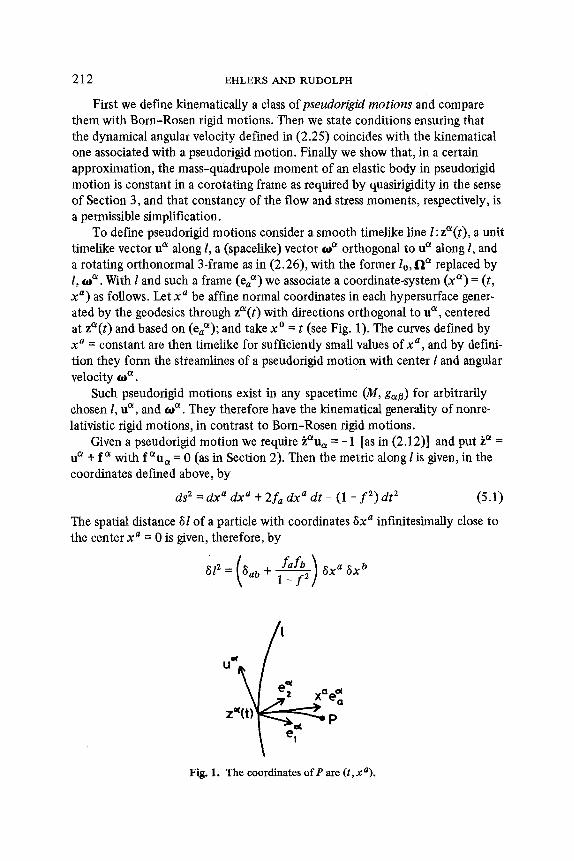
To define pseudofigid motions consider a smooth timelike line l: zS(t), a unit timelike vector u s along l, a (spacelike) vector ta s orthogonal to u a along l, and a rotating orthonormal 3-flame as in (2.26), with the former 10, [1 s replaced by l, to s . With l and such a frame (ea a) we associate a coordinate-system (x s ) = (t, x a ) as follows. Let x a be affine normal coordinates in each hypersurface generated by the geodesics through zS(t) with directions orthogonal to u s , centered at za(t) and based on (eaS); and take x ~ = t (see Fig. 1). The curves defined by x a = constant are then timelike for sufficiently small values o f x a, and by definition they form the streamlines of a pseudofigid mot ion with center 1 and angular velocity ta ~.

Such pseudofigid motions exist in any spacetime (M, gs~) for arbitrarily chosen l, u s , and ta ~ . They therefore have the kinematical generality of nonrelativistic rigid motions, in contrast to Born-Rosen rigid motions.

Given a pseudofigid mot ion we require ~aua --- - 1 [as in (2.12)] and put ~.~ = u s + f a with f ~ u a = 0 (as in Section 2). Then the metric along l is given, in the coordinates defined above, by

ds 2 = d x a d x a + 2f= d x a d t - (1 - f 2 ) d t 2 (5.1)

The spatial distance 61 of a particle with coordinates 8 x a infinitesimally close to the center x a = 0 is given, therefore, by

�9 (

I

z=C(t) . . . ~ = ~ , p

e t

Fig. 1. The coordinates of P are (t, xa) .


Since the 6x a are constant, the rate of change of 5l is determined by

(6l)_Z ~ t (Sl:Z)= 2 (6l)" = [~_~ ( faf~2/] 6X a 6Xb. (5.2) \1 - f / j

This equation shows: If fe = 0, i.e., if ~e = u s, then the rate of strain of a pseudorigid motion vanishes along the center l. Moreover, (5.2) shows that the rate of strain is small if fu is small and changes only slowly. Because of continuity we obtain: A pseudorigid mo t ion is nearly B o r n - R o s e n rigid i f ~. ~ - u s = f e is small, changes s lowly only , and provided the body is small.

The preceding consideration applies in particular to the case where l = 10 is the center-of-mass world line of a body defined in Section 2, in which case fu is given by (2.17) and estimated in (2.22).

For the remainder of this section we assume that the matter constituting the body under consideration has a stress-energy tensor of the form

T e # = p w ~ w ~ + pen (5.3)

with

w e w ~ = - 1, pe~w~ --- 0 (5.4)

and that the streamlines generated by w e form a pseudorigid motion with center 10 and some not yet specified angular velocity to ~.

In order to find conditions under which the dynamical angular velocity IIe defined in (2.25) coincides approximately with the kinematical angular velocity oj e used to define the internal motion of the body we introduce, besides the "corotating" coordinates (t , x a) employed to construct pseudorigid motions, another set ( t , X a) of "nonrotating" coordinates. They are defined in the same manner as (t , xa ) , except that the angular velocity to e used in the definition of the x a is replaced by the zero vector.

The transformation from co-rotating to non-rotating coordinates is X a = D a a ( t ) x b where the rotation matrix Dab is related to off as in nonrelativistic kinematics. Using the symbol _o to emphasize that an equation refers to such nonrotating coordinates ( t , X a) we note that along lo

ds 2 o= d X a d X a + 2fa d X a d t - (1 - f Z ) d t 2 (5.5)

and for a pseudorigid motion

dt (5.6) dt wa o= eabcwbXC d---~ w o o d r '

where ~- is the proper time and e . . . is the standard permutation symbol. If we consider either a test body in a slowly varying external field or a mas-

sive body with M]r < < 1 (and thus also dt]d7 ~ 1), then (5.5) holds approximately not only on lo but everywhere in the body. This follows from the Taylor


series for gag which can be found by the same technique that is used in the case of Fermi coordinates. We obtain from (5.6)

Wo ~ -1, w a ~ eabccobX c (5.7)

This second equation (5.4) then implies

poo ~ pab(cor)2,paO ~ pab ebcacocxa

whereas (5.3) and (5.6) give

TOO ,~ p + pOO,

Toa ~, peabccobX e + pOa

Assuming

Ipabl <</9 (5.8)

we infer from the preceding relations

TOO ,&. p, T ~ ,~ peabccobX c (5.9)

Dixon's definition of angular momentum reads, in the coordinates used here, as

S o o S a ~ 1 ~a o b c = O , = ~ b c o

with

f XICHbl a, Ta'o' ' 2 f VtCHOlo,TO'O' Sb c =o 2 (_g)l/2 d3X + (_g)l/2 daX , (5.10)

H ~ , is a bitensor associated with Jacobi's equation, defined in [1 ]. According to equations (5.9), (5.10), and the remarks made in connection with the definition of I ap [see the sentences following (2.24)], the "Newtonian" relation S ~ ___o I~#cor will hold approximately provided that

Hba , "~ 6ha (5.11)

and that the second contribution to the fight-hand side of (5.10) is negligible compared to the first one.

In the case of a test body these conditions can be verified by means of a Taylor expansion of H~#, in the coordinates X ~. Such an expansion shows that (5.11) holds, and that the lowest-order term ofHbo , is cubic in the X a, with co- efficients given by R~#.r8 ;e. If we write L and d for a typical radius of curvature of the external field and a typical length scale on which L changes, respectively, then the second term of (5.10) differs from the first one by a factor of the order

r/d(r/L )2(cor) -1

which is usually much less than one if the test body approximation applies.


For a heavy, slowly rotating body with M]r < < 1 the ratio under discussion is of the order M]r; i.e., it is again negligible.

Under the assumptions introduced so far the kinematical angular velocity o~ ~ is related to the angular momentum S ~, the tensor of inertia I ~t~, and the CM-4- velocity u s precisely like the dynamical angular velocity 1~ ~ of Section 2, i.e.,

For very compact bodies wi thM]r ~ 1 the second term of (5.10) might not be negligible. A "tensor of inertia" satisfying (2.25) can then still be defined, but its dependence on the structure of the body need not be the one given by equation (2.23a, b), but has to be derived from the theory of stellar structure (see, e.g. [17] ).

We now estimate the rate of change of the corotating tetrad components of the mass quadrupole moment m ~t~ along lo. Let -~ indicate that an equation refers to corotating coordinates (t, x a). Then m ~ -~ 0, and the spatial tetrad components are identical to the natural (coordinate) components m ab. Evaluation of m ab as defined by Dixon under the assumptions made in the derivation of ~ 1~ ~ leads to

Therefore

mab .~ f xaxbp(wO)2 (_ g)l/z d3x

d a b ~ f xaxb (~lat)([-g] 1/2 pwO)wOd3x + f xaxb (_ g) l / 2 pw o (awo/~t)d3 X m

The energy balance equation of elasticity theory is

1 a ([-g] ' /=pw ~ *-_ Vu(pw u) = -pU~eu~

(_g)1/2 at

where | is the rate-of-strain tensor. The latter is nearly zero for a small body in pseudo-rigid motion as shown above in connection with equation (5.2). Hence the first contribution to (5.4) is very small. Moreover, w ~ ~ (1 - f 2 ) - , / 2 as is seen from (5.1). Therefore, under the assumptions made already (which include that f changes slowly), the second contribution to (5.4) is small, too. Altogether, then, we have shown that m ab is nearly constant, as required by (approximate) quasirigidity.

Analogous statements about the flow and stress-moments defined in (4.10) and (4.11), respectively, do not hold. This is irrelevant for the usefulness of quasirigidity as an approximation, however, for the following reason. Insertion of the decomposition (4.12) of the quadrupole-moment into the force and torque (4.3) and (4.4), respectively, shows that for a Newtonian curvature tensor (see, e.g. [5] ), only the contributions containing m ~t3 are different from zero, and that even for moderately relativistic fields the rn contributions to the


force and torque clearly dominate the 7r and r contributions. Therefore, using for ~r and r quantities with the wrong time dependence introduces no significant errors into the equations of motion, except possibly for extremely relativistic bodies in highly relativistic motions. In particular, taking 7r and r to be constant as required in the definition of quasirigidity (or discarding the corresponding terms altogether) is an admissible simplification under most circumstances.

w Concluding Remarks

The attempt made in this paper to contribute to the development of a relativistic dynamics of gravitationally interacting bodies was guided by the ques- tion: How can one augment or specialize Dixon's general balance equations (1.5) and (1.6) such as to obtain laws of motion which determine, relatively to a given metric, a motion uniquely in terms of initial data. One step in this direction was the derivation of the momentum-velocity equation (2.17), another one was the definition of quasirigid motions and the investigation of its consequences in Sec- tion 3 and the analysis of its physical justification in Section 5. The first step hardly requires further discussion or modification. The second one, however, should only be considered as illustrating, by way of an example, how one might proceed. Our definition of quasirigidity is a specialization of Dixon's "dynamical rigidity" [1]. The specialization consists of the choice (2.24), (2.25), and (2.26) of that "comoving" frame with respect to which "rigidity" is defined. It appears to us that the comoving frame ought to be defined in terms of the set (2.18) of reduced CM moments since these contain the complete information about T ag ; it should not be introduced independently. However, our choice of the comoving frame may be too special for extremely relativistic systems. Other choices could perhaps be obtained from the theory of highly compact, rotating bodies.

Granted one has found suitable laws of motion relatively to a given metric, there remains the even more difficult problem to express the metric, by means of field equations and boundary conditions, in terms of source variables, and to insert these expressions into the laws of motion to obtain the "equations of motion" [18]. One major obstacle here is that a useful covariant decomposition of the total metric and (or) connection into a self field and an incident field has not yet been found. This basic difficulty presented itself in various parts of this paper. Perhaps one could use equation (3.7), together with conditions on the background metric and boundary conditions, to associate a "self-connection" with each body. A self-field-analysis seems indispensible for the introduction of a "point particle" model into general relativity, for a justification, on the basis of field equations [and not only on the basis of (1.1) for a given metric] of the geodesic law for bodies like planets or stars (see Section 4), and for the definition and computation of radiation reaction forces. It is not clear at present whether for these purposes one has to resort to approximation methods from the begin-


ning, or whether the rigorous Dixon approach can be extended in this direction.

It seems worthwhile making corresponding at tempts. 7

Acknowledgments

The authors would like to thank Dr. B. Carter and Dr. W. G. Dixon for stim- ulating discussions. Financial support by the Deutsche Forschungsgemeinschaft is gratefully acknowledged.

Note Added in Proof

Some results and problems considered in this paper have been incorporated, partly with extensions, into Dixon's lectures at the E. Fermi school (1976); see the proceedings of that school (to appear soon).

References

1. Dixon, W. G. (1970).Proc. R. Soc. London, Set. A 314,499. 2. Dixon, W. G. (1970).Proc. Ro Soc. London, Ser. A 319,509~ 3. Dixon, W. G. (1973). Gen. Rel. Gray. 4, 199. 4. Dixon, W. G. (1974).Philos. Trans. R. Soc. London, Set. A 277,59. 5. Misner, C. W., Tho~ne, K. S., and Wheeler, J. A. (1971). Gravitation. (San Francisco). 6. Madore, J. (1966). C. R. Acad. Sei.,Ser. A 263, 746. 7. Beiglb6ck, W. (1967). Commun. Math. Phys. 5,106. 8. Geroch, R., and Soo Yang, P. (1975). J. Math. Phys. 16, 65. 9. Synge, J. L. (1956). Relativity: The Special Theory. (Amsterdam).

10. Schild, A. (1967). in Lectures on GeneralRelativity, J. Ehlers, ed. "Lectures in Applied Mathematics," Vol. 8, pp. 17-20. (American Mathematical Society).

11. Munk, W. H. and MacDonald, G. J. F. (1960), The Rotation of the Earth. (Cambridge), p. 10.

12. Foek, V. A. (1959). The Theory of Space, Time and Gravitation. (New York). 13. D'Eath, P. D. (1975). Phys. Rev. D 11, 1387; 12, 2183. 14. Carter, B., and Quintana, H. (1972). Proc. R. Soc. London, Set. A 331, 57. 15. Carter, B. (1973).Phys. Rev. D 7, 1590. 16. Wahlquist, H. D., and Estabrook, F. B. (1966). Z Math. Phys. 7, 894. 17. Cohen, J. M. (1970).Astrophys. Space Sci. 6,263. 18. Infeld, L., and Plebanski, J. (1960). Motion and Relativity. (New York). 19. Tod, K. P., and de Felice, F. (1976). "Spinning Test Particles in the Field of a Black

Hole." (Prepfint, University of Padova).

7A proposal in this direction is described in Dixon's lectures at the Varenna School in 1976 and will appear in the proceedings of that school.

Date post:	12-Feb-2017
Category:	Documents
Upload:	phamkhue
View:	226 times
Download:	2 times

Dynamics of extended bodies in general relativity center-of-mass ...

Documents