DYNAMICS OF FLUID-CONVEYING TIMOSHENKO PIPES A Thesis by RYAN CURTIS PETRUS Submitted to the Office of Graduate Studies of Texas A&M University in partial fulfillment of the requirements for the degree of MASTER OF SCIENCE May 2006 Major Subject: Mechanical Engineering
Transcript
DYNAMICS OF FLUID-CONVEYING TIMOSHENKO PIPES
A Thesis
by
RYAN CURTIS PETRUS
Submitted to the Office of Graduate Studies of Texas A&M University
in partial fulfillment of the requirements for the degree of
MASTER OF SCIENCE
May 2006
Major Subject: Mechanical Engineering
DYNAMICS OF FLUID-CONVEYING TIMOSHENKO PIPES
A Thesis
by
RYAN CURTIS PETRUS
Submitted to the Office of Graduate Studies of Texas A&M University
in partial fulfillment of the requirements for the degree of
MASTER OF SCIENCE
Approved by: Chair of Committee, J.N. Reddy Committee Members, Ray M. Bowen Jose Roesset Head of Department, Dennis L. O’Neal
May 2006
Major Subject: Mechanical Engineering
iii
ABSTRACT
Dynamics of Fluid-Conveying Timoshenko Pipes. (May 2006)
Ryan Curtis Petrus, B.S., B.S., Louisiana Tech University
Chair of Advisory Committee: Dr. J.N. Reddy
Structures conveying mass lose stability once the mass exceeds a certain critical
velocity. The type of instability observed depends on the nature of the supports that the
structure has. If the structure (beam or pipe) is cantilevered (thereby deeming it a non-
conservative system), “garden-hose-like” flutter instability is observed once a critical
velocity is exceeded. When studying the flutter instability of a cantilevered pipe
(including shear deformation) by strictly a linear theory, it has been demonstrated
through numerical integration that the values of the critical velocity are only valid for
small values of the mass ratio (mass of the fluid divided by the total mass)
(approximately 0.1β < ). This fact is also true if shear deformation is neglected. Also,
linear theory predicts the pipe to oscillate unboundedly as time progresses, which is
physically impossible. Therefore, shortly after the pipe goes unstable, the linear theory
is no longer applicable. If non-linear terms are taken into account from the beginning, it
can be shown that the pipe oscillates into a limit cycle.
iv
This thesis, along with the rest of my degrees, is dedicated to my Dad. He has
supported every decision I have made throughout college (and life) and he has helped
me in every way possible. He has always taught me to work hard at everything and
reach every goal set.
v
ACKNOWLEDGEMENTS
When I came to Texas A&M University in 2004, I had no background in
mechanical engineering and thus, had no particular interests. Because I had to be taught
from square one, I would like to acknowledge every professor that helped me gain
knowledge (and interest) in mechanics and dynamics. Therefore, I would like to give
my appreciation to Professors Reddy, Srinivasa, Bowen, Palazzolo, and Roesset.
vi
TABLE OF CONTENTS
Page ABSTRACT .............................................................................................................. iii DEDICATION .......................................................................................................... iv ACKNOWLEDGEMENTS ...................................................................................... v TABLE OF CONTENTS .......................................................................................... vi LIST OF TABLES .................................................................................................... viii LIST OF FIGURES................................................................................................... x CHAPTER I INTRODUCTION............................................................................. 1 II EARLY HISTORY AND LITERATURE REVIEW ....................... 5 III ENERGY FORMULATION AND EQUATIONS OF MOTION.... 8 A. Displacements and Strains..................................................... 8 B. Virtual Work.......................................................................... 10 C. Non-Dimensional Equations of Motion ................................ 17 IV EIGENVALUE PROBLEM AND APPROXIMATE SOLUTION . 20 A. Eigenvalue Problem .............................................................. 20 B. Boundary Conditions ............................................................. 21 C. The Bubnov-Galerkin Weighted Residual Method ............... 24 D. Basis Functions...................................................................... 28 V DETERMINATION OF THE CRITICAL VELOCITIES ............... 31 A. Rotary Inertia......................................................................... 33 B. Routh-Hurwitz Stability Criteria ........................................... 33 C. Determination of the Critical Velocities by Trigonometric\Hyperbolic Basis Functions for a Thin Beam .......................................... 35
vii
CHAPTER Page D. Determination of the Critical Velocities by Polynomial Basis Functions for a Thin Beam .......................................... 50 E. Determination of the Critical Velocities by Trigonometric\Hyperbolic Basis Functions for a Moderately Thick and Thick Beam........................................ 59 F. Determination of the Critical Velocities by Polynomial Basis Functions for a Moderately Thick and Thick Beam..... 72 VI APPROXIMATE SOLUTION OF THE TIME-DEPENDENT EQUATIONS OF MOTION............................................................. 85 A. The Weak Form..................................................................... 85 B. Interpolation Functions.......................................................... 88 C. Assembly of Global Matrices and Imposition of Boundary Conditions ............................................................................. 94 D. The Newmark Method Time Scheme ................................... 97 E. Numerically Integrated Results ............................................. 99 VII CONCLUSION ................................................................................. 117 REFERENCES ..................................................................................................... 120 APPENDIX A ROUTH-HURWITZ STABILITY CRITERIA .......................... 123 APPENDIX B DERIVATION OF SUPER-CONVERGENT SHAPE FUNCTIONS .............................................................................. 126 APPENDIX C 1-D FINITE ELEMENT PROGRAM......................................... 129 VITA ..................................................................................................... 136
viii
LIST OF TABLES
TABLE Page 5.1 Natural frequencies (without fluid) for various beam thicknesses................ 32 5.2 Dimensionless critical velocities for the two-term trigonometric/hyperbolic approximation ( 5~ 10Λ ) ............................................................................... 37 5.3 Roots of equation (5.11) for 0.1β = ............................................................ 41 5.4 Dimensionless critical velocities for the four-term trigonometric/hyperbolic approximation ( 5~ 10Λ ) .............................................................................. 42 5.5 Dimensionless critical velocities for the five-term trigonometric/hyperbolic approximation ( 5~ 10Λ ) .............................................................................. 47 5.6 Dimensionless critical velocities for the two-term polynomial approximation ( 5~ 10Λ ) ............................................................................... 51 5.7 Dimensionless critical velocities for the four-term polynomial approximation ( 5~ 10Λ ) ............................................................................... 53 5.8 Dimensionless critical velocities for the five-term polynomial approximation ( 5~ 10Λ ) ............................................................................... 55 5.9 Dimensionless critical velocities for the two-term trigonometric/hyperbolic approximation ( 310Λ ∼ ) ............................................................................... 60 5.10 Dimensionless critical velocities for the two-term trigonometric/hyperbolic approximation ( 210Λ ∼ ) ............................................................................... 61 5.11 Dimensionless critical velocities for the four-term trigonometric/hyperbolic approximation ( 310Λ ∼ ) ............................................................................... 66 5.12 Dimensionless critical velocities for the four-term trigonometric/hyperbolic approximation ( 210Λ ∼ ) ............................................................................... 67 5.13 Dimensionless critical velocities for the two-term polynomial approximation ( 310Λ ∼ ) ............................................................................... 73
ix
TABLE Page 5.14 Dimensionless critical velocities for the two-term polynomial approximation ( 210Λ ∼ ) ............................................................................... 74 5.15 Dimensionless critical velocities for the four-term polynomial approximation ( 310Λ ∼ ) ............................................................................... 79 5.16 Dimensionless critical velocities for the four-term polynomial approximation ( 210Λ ∼ ) ............................................................................... 80
x
LIST OF FIGURES
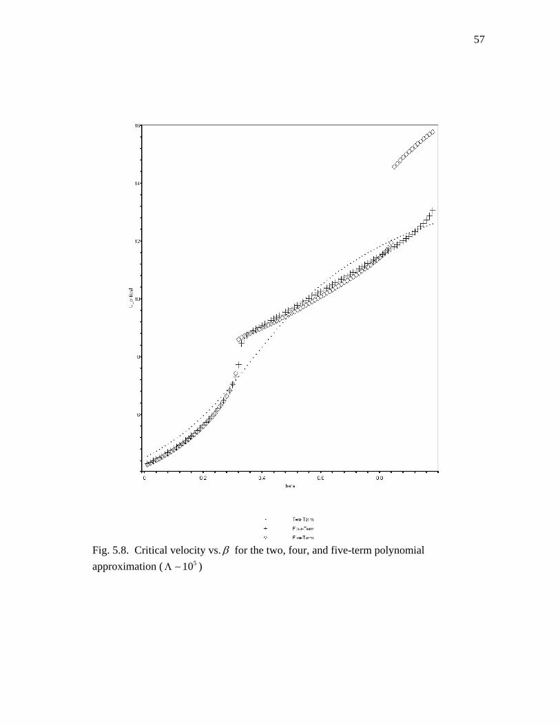
FIGURE Page 3.1 A typical deformed element according to Timoshenko beam theory ........... 9 3.2 A typical deformed element conveying fluid according to Euler-Bernoulli beam theory......................................................................... 11 5.1 Critical velocity vs.β for the two-term trigonometric/hyperbolic approximation ( 510Λ ∼ ) .............................................................................. 38 5.2 Critical velocity vs.β for the four-term trigonometric/hyperbolic approximation ( 510Λ ∼ ) ............................................................................... 43 5.3 Critical velocity vs.β for the five-term trigonometric/hyperbolic approximation ( 510Λ ∼ ) ............................................................................... 48 5.4 Critical velocity vs.β for the two, four, and five-term trigonometric/hyperbolic approximation ( 510Λ ∼ ) ...................................... 49 5.5 Critical velocity vs.β for the two-term polynomial approximation ( 510Λ ∼ ) 52 5.6 Critical velocity vs.β for the four-term polynomial approximation ( 510Λ ∼ ) 54 5.7 Critical velocity vs.β for the five-term polynomial approximation ( 510Λ ∼ ) 56 5.8 Critical velocity vs.β for the two, four, and five-term polynomial approximation ( 510Λ ∼ ) ............................................................................. 57 5.9 Critical velocity vs.β for the two-term trigonometric/hyperbolic approximation for 310Λ ∼ and 510Λ ∼ ....................................................... 62 5.10 Critical velocity vs. β for the two-term trigonometric/hyperbolic approximation for 210Λ ∼ and 510Λ ∼ ....................................................... 63 5.11 Critical velocity vs. β for the two-term trigonometric/hyperbolic approximation for 210Λ ∼ , 310Λ ∼ , and 510Λ ∼ ....................................... 64
xi
FIGURE Page 5.12 Critical velocity vs. β for the four-term trigonometric/hyperbolic approximation for 310Λ ∼ and 510Λ ∼ ....................................................... 68 5.13 Critical velocity vs.β for the four-term trigonometric/hyperbolic approximation for 210Λ ∼ and 510Λ ∼ ....................................................... 69 5.14 Critical velocity vs.β for the four-term trigonometric/hyperbolic approximation for 210Λ ∼ , 310Λ ∼ , and 510Λ ∼ ....................................... 70 5.15 Critical velocity vs.β for the two-term polynomial approximation for 310Λ ∼ and 510Λ ∼ ............................................................................... 75 5.16 Critical velocity vs.β for the two-term polynomial approximation for 210Λ ∼ and 510Λ ∼ ............................................................................... 76 5.17 Critical velocity vs.β for the two-term polynomial approximation for 210Λ ∼ , 310Λ ∼ , and 510Λ ∼ ............................................................... 77 5.18 Critical velocity vs.β for the four-term polynomial approximation for 310Λ ∼ and 510Λ ∼ ............................................................................... 81 5.19 Critical velocity vs.β for the four-term polynomial approximation for 210Λ ∼ and 510Λ ∼ ............................................................................... 82 5.20 Critical velocity vs.β for the four-term polynomial approximation for 210Λ ∼ , 310Λ ∼ , and 510Λ ∼ ............................................................... 83 6.1 2 1N−Δ vs. τ for 4.29u = , 0.01β = , and 510Λ ∼ ........................................ 100 6.2 2 1N−Δ vs. τ for 4.30u = , 0.01β = , and 510Λ ∼ ........................................ 101 6.3 2 1N−Δ vs. τ for 4.75u = , 0.05β = , and 510Λ ∼ ........................................ 102 6.4 2 1N−Δ vs. τ for 4.76u = , 0.05β = , and 510Λ ∼ ........................................ 102 6.5 2 1N−Δ vs. τ for 5.59u = , 0.10β = , and 510Λ ∼ ........................................ 103
xii
FIGURE Page 6.6 2 1N−Δ vs. τ for 5.60u = , 0.10β = , and 510Λ ∼ ........................................ 104 6.7 2 1N−Δ vs. τ for 8.78u = , 0.20β = , and 510Λ ∼ ........................................ 105 6.8 2 1N−Δ vs. τ for 8.79u = , 0.20β = , and 510Λ ∼ ........................................ 105 6.9 2 1N−Δ vs. τ for 4.29u = , 0.01β = , and 310Λ ∼ ........................................ 107 6.10 2 1N−Δ vs. τ for 4.30u = , 0.01β = , and 310Λ ∼ ........................................ 107 6.11 2 1N−Δ vs. τ for 5.59u = , 0.10β = , and 310Λ ∼ ........................................ 108 6.12 2 1N−Δ vs. τ for 5.60u = , 0.10β = , and 310Λ ∼ ........................................ 109 6.13 2 1N−Δ vs. τ for 8.75u = , 0.20β = , and 310Λ ∼ ........................................ 110 6.14 2 1N−Δ vs. τ for 8.76u = , 0.20β = , and 310Λ ∼ ........................................ 110 6.15 2 1N−Δ vs. τ for 4.22u = , 0.01β = , and 210Λ ∼ ........................................ 111 6.16 2 1N−Δ vs. τ for 4.23u = , 0.01β = , and 210Λ ∼ ........................................ 112 6.17 2 1N−Δ vs. τ for 5.51u = , 0.10β = , and 210Λ ∼ ........................................ 113 6.18 2 1N−Δ vs. τ for 5.52u = , 0.10β = , and 210Λ ∼ ........................................ 113 6.19 2 1N−Δ vs. τ for 8.46u = , 0.20β = , and 210Λ ∼ ........................................ 114 6.20 2 1N−Δ vs. τ for 8.47u = , 0.20β = , and 210Λ ∼ ........................................ 115
1
CHAPTER I
INTRODUCTION
The stability of structures conveying mass has interested engineers over the past
century; such applications include exhaust pipes, stacks of flue gases, air-conditioning
ducts, offshore piping, traveling chains, nuclear reactors, and jet pumps. A particular
area of interest that has received attention over the past few decades is the stability of
elastic pipes conveying fluid. The dynamic interaction between the fluid (water, gas,
etc.) and the pipe causes energy to be transferred to the pipe, and after a sufficient
amount of energy exchange, stability of the pipe is lost.
When formulating the equations of motion for elastic pipes, three accelerations
associated with the inertial axial transport of mass appear: (i) transverse acceleration of
the fluid, (ii) the Coriolis acceleration associated with the change of angular velocity,
and (iii) the centripetal acceleration associated with the deformed (curved) shape of the
pipe. The new forces, respectively, are
2
02transverse f
wF mt
∂=
∂ (1.1)
2
02Coriolis fwF m
t x∂
=∂ ∂
(1.2)
2
2 02centripetal f
wF m vx
∂=
∂ (1.3)
This thesis follows the style of Journal of Sound and Vibration.
2
where fm is the mass per unit length of the fluid, 0w is the transverse deflection of the
beam, and v is the magnitude of the fluid’s velocity vector. These new forces cause
different types of instability depending solely on the boundary conditions present.
Once these linear equations of motion are formulated, the free-vibration
eigenvalue problem is formulated. The imposition of the boundary conditions (simply-
supported or cantilevered) will now determine what type of instability is present. If the
beam is simply-supported/cantilevered, it can loose stability by buckling/flutter. When
the beam is simply supported, the buckling phenomenon is characterized by the
domination of the stiffening centripetal force (buckling load) over the Coriolis restoring
(damping) force for some critical velocity. When the beam is cantilevered, the flutter
phenomenon is characterized by the combination of the work done by the Coriolis force
and extra energy added by the fluid; these two energy inputs cause negative damping to
occur at some critical velocity. Paidoussis [1] stated (proved by Benjamin [2]) that the
rate of work done by the fluid forces over a period of oscillation is
2
000
L
fwdW m v w dx
dt t t x∂ ∂ ∂⎛ ⎞= − +⎜ ⎟∂ ∂ ∂⎝ ⎠∫ (1.4)
where 0w is the transverse displacement, fm is the mass per unit length of the fluid, and
v is the velocity of the fluid. The work done over a cycle T is thus
For each value of β (0 0.99)β≤ ≤ , equation (5.8) can be solved and the smallest
positive real value of u gives the value for the critical velocity. For example,
when 0.1β = ,
1
2
3
4
5
6
7
8
9
10
u =0.0u =0.0u =-2.449382666+4.204079422iu =2.449382666-4.204079422iu =-2.449382666-4.204079422i u =2.449382666+4.204079422i u =-4.702764105u =4.702764105u =-30.59900565u =30.59900565
(5.9)
hence, 4.702764105criticalU = . Table 5.2 gives the critical velocities for all values of β .
Figure 5.1 shows the plot of criticalU vs. β .
37
Table 5.2 Dimensionless critical velocities for the two-term trigonometric\hyperbolic approximation ( 5~ 10Λ )
β critU β
critU β critU β
critU
0.01
0.02
0.03
0.04
0.05
0.06
0.07
0.08
0.09
0.10
0.11
0.12
0.13
0.14
0.15
0.16
0.17
0.18
0.19
0.20
0.21
0.22
0.23
0.24
0.25
4.221410035
4.268771126
4.317529487
4.367740138
4.419459729
4.472746378
4.527659472
4.584259397
4.642607188
4.702764105
4.764791094
4.828748140
4.894693487
4.962682710
5.032767630
5.104995051
5.179405323
5.256030722
5.334893654
5.416004699
5.499360544
5.584941825
5.672710978
5.762610176
5.854559462
0.26
0.27
0.28
0.29
0.30
0.31
0.32
0.33
0.34
0.35
0.36
0.37
0.38
0.39
0.40
0.41
0.42
0.43
0.44
0.45
0.46
0.47
0.48
0.49
0.50
5.948455211
6.044169059
6.141547449
6.240411904
6.340560148
6.441768121
6.543792900
6.646376457
6.749250117
6.852139522
6.954769880
7.056871200
7.158183276
7.258460165
7.357473988
7.455017896
7.550908173
7.644985446
7.737115086
7.827186894
7.915114137
8.000832196
8.084296802
8.165482117
8.244378683
0.51
0.52
0.53
0.54
0.55
0.56
0.57
0.58
0.59
0.60
0.61
0.62
0.63
0.64
0.65
0.66
0.67
0.68
0.69
0.70
0.71
0.72
0.73
0.74
0.75
8.320991370
8.395337364
8.467444262
8.537348310
8.605092803
8.670726635
8.734303028
8.795878424
8.855511527
8.913262473
8.969192158
9.023361655
9.075831746
9.126662519
9.175913095
9.223641338
9.269903704
9.314755086
9.358248708
9.400436071
9.441366892
9.481089108
9.519648868
9.557090527
9.593456701
0.76
0.77
0.78
0.79
0.80
0.81
0.82
0.83
0.84
0.85
0.86
0.87
0.88
0.89
0.90
0.91
0.92
0.93
0.94
0.95
0.96
0.97
0.98
0.99
1.00
9.628788291
9.663124514
9.696502965
9.728959665
9.760529104
9.791244310
9.821136892
9.850237104
9.878573901
9.906174991
9.933066884
9.959274954
9.984823481
10.00973571
10.03403388
10.05773930
10.08087236
10.10345260
10.12549872
10.14702867
10.16805960
10.18860801
10.20868968
10.22831975
10.24751276
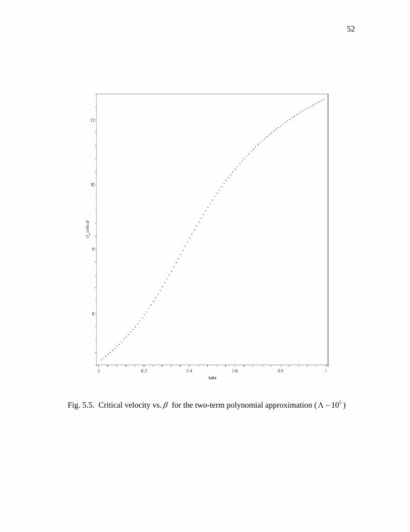
38
Fig. 5.1. Critical velocity vs. β for the two-term trigonometric\hyperbolic approximation ( 510Λ ∼ )
39
2. Four-Term Approximation
For the N=4 ( 8, 0)n σ= = case, the basis functions are once again calculated
Once again, all initial conditions will be taken as zero. Equations (6.51)-(6.54) are
repeated (in a loop) for however long desired. For the problem at hand, the system will
go unstable or stable in a short amount of time.
E. Numerically Integrated Results
1. Numerically Integrated Results for a Thin Beam
Numerically integrating (6.45) through use of the Newmark time scheme ((6.51)-
(6.55)) was done by a program written in MATLAB 7.0.1 (see Appendix C). The non-
dimensional fixed parameter values used were 510Λ ∼ , 0.01 0.20β≤ ≤ , 40 1.0 10xγ −= ,
and 0σ = . The reasoning behind stopping at 0.2β = is to steer clear of the “jumps” and
divergence present in the higher order approximations (trigonometric\hyperbolic and
polynomial). After these values were fixed, the velocity u was varied until the onset of
instability. The finite element values used in the program were 31.0 10xτ −Δ = ,
100
{ } { }0
0Δ = , { } { }0
0Δ = , and { } { }0
0Δ = with 50 elements integrated over 100 non-
dimensional time units. Once { }s
Δ ( )1, 2,s = … was obtained, the value of the deflection
( )2 1N s−Δ ( )0,1, 2s = … was plotted versus τ for each time step.
The first example is a thin beam ( )510Λ ∼ with a very small mass ratio 0.01β = .
When 4.29u = , the response was stable as shown in Figure 6.1 and when 4.30u = , the
response was unstable as shown in Figure 6.2. Therefore, the critical velocity can be
approximated as 4.295u = . The percent error between this value and the value obtained
from the five-term trigonometric\hyperbolic approximation ( 4.234u = ) in Table 5.5 and
the five-term polynomial approximation ( 4.272u = ) in Table 5.8 is 1.4% and 0.5%
respectively.
Fig. 6.1. 2 1N −Δ vs. τ for 4.29u = , 0.01β = , and 510Λ ∼
101
Fig. 6.2. 2 1N −Δ vs. τ for 4.30u = , 0.01β = , and 510Λ ∼ When 0.05β = Figure 6.3 shows the response to be stable when 4.75u = and
Figure 6.4 shows the response to be unstable at 4.76u = ; therefore, the critical velocity
can be approximated as 4.755u = . Compared with the value obtained in Table 5.5
( 4.441u = ) and in Table 5.8 ( 4.478u = ), the percent error is 6.6% and .5.8%
respectively.
102
Fig. 6.3. 2 1N −Δ vs. τ for 4.75u = , 0.05β = , and 510Λ ∼
Fig. 6.4. 2 1N −Δ vs. τ for 4.76u = , 0.05β = , and 510Λ ∼
103
When 0.10β = Figure 6.5 shows the response to be stable when 5.59u = and
Figure 6.6 shows the response to be unstable at 5.60u = ; therefore, the critical velocity
can be approximated as 5.595u = . Compared with the value obtained in Table 5.5
( 4.746u = ) and in Table 5.8 ( 4.781u = ), the percent error is 15.2% and .14.6%
respectively.
Fig. 6.5. 2 1N −Δ vs. τ for 5.59u = , 0.10β = , and 510Λ ∼
104
Fig. 6.6. 2 1N −Δ vs. τ for 5.60u = , 0.10β = , and 510Λ ∼ When 0.20β = Figure 6.7 shows the response to be stable when 8.78u = and
Figure 6.8 shows the response to be unstable at 8.79u = ; therefore, the critical velocity
can be approximated as 8.785u = . Compared with the value obtained in Table 5.5
( 5.585u = ) and in Table 5.8 ( 5.601u = ), the percent error is 36.4% and .36.2%
respectively.
105
Fig. 6.7. 2 1N −Δ vs. τ for 8.78u = , 0.20β = , and 510Λ ∼
Fig. 6.8. 2 1N −Δ vs. τ for 8.79u = , 0.20β = , and 510Λ ∼ As seen from Figures 6.1-6.8, the values of the critical velocities obtained from
the Bubnov-Galerkin approximation (trigonometric\hyperbolic and polynomial) agree
very well for 0.01 0.05β≤ ≤ , fair for 0.10β = , and poor for 0.20β = compared with
106
the exact numerical integration critical velocities. It was expected from the graphs
created in the previous chapter that the results for 0.3β > would be poor but unexpected
for 0.2β = . This discrepancy is due firstly to the fact that the Bubnov-Galerkin
approximation is simply an approximation and secondly due to the fact that the basis
functions used in the Bubnov-Galerkin approximation were obtained from the non-fluid
differential equations; i.e. the boundary conditions (essential and natural) were not
satisfied exactly.
2. Numerically Integrated Results for a Moderately Thick and Thick Beam
The procedure for numerically integrating the time-dependent differential
equations for a moderately thick and thick beam will be identical to the procedure for a
thin beam. Once again, the non-dimensional fixed material parameter values used
were 2 310 ,10Λ ∼ , 0.01 0.20β≤ ≤ , 40 1.0 10xγ −= , and 0σ = . For the sake of brevity,
only three values of the mass ratio will be considered, 0.01,0.10,0.20β = The finite
element values used again were 31.0 10xτ −Δ = , { } { }0
0Δ = , { } { }0
0Δ = , and { } { }0
0Δ =
with 50 elements integrated over 100 non-dimensional time units.
When 0.01β = ( 310Λ ∼ ), Figure 6.9 shows the response to be stable when
4.29u = and Figure 6.10 shows the response to be unstable at 4.30u = ; therefore, the
critical velocity can be approximated as 4.295u = . This result is exactly the
numerically integrated result when 510Λ ∼ . Compared with the value obtained in Table
5.11 for the four-term trigonometric\hyperbolic approximation ( 4.186u = ) and in Table
107
5.15 for the four-term polynomial approximation ( 4.298u = ), the percent error is 6.6%
and 27.0 10x − % respectively.
Fig. 6.9. 2 1N −Δ vs. τ for 4.29u = , 0.01β = , and 310Λ ∼
Fig. 6.10. 2 1N −Δ vs. τ for 4.30u = , 0.01β = , and 310Λ ∼
108
When 0.10β = ( 310Λ ∼ ), Figure 6.11 shows the response to be stable when
5.59u = and Figure 6.12 shows the response to be unstable at 5.60u = ; therefore, the
critical velocity can be approximated as 5.595u = . This result is again exactly the result
obtained when 510Λ ∼ Compared with the value obtained in Table 5.11 for the four-
term trigonometric\hyperbolic approximation ( 4.691u = ) and in Table 5.15 for the four-
term polynomial approximation ( 4.805u = ), the percent error is 16.2% and 14.1%
respectively.
Fig. 6.11. 2 1N −Δ vs. τ for 5.59u = , 0.10β = , and 310Λ ∼
109
Fig. 6.12. 2 1N −Δ vs. τ for 5.60u = , 0.10β = , and 310Λ ∼ When 0.20β = ( 310Λ ∼ ), Figure 6.13 shows the response to be stable when
8.75u = and Figure 6.14 shows the response to be unstable at 8.76u = ; therefore, the
critical velocity can be approximated as 8.755u = . This result are very close to the
result obtained when 510Λ ∼ ( 8.785u = ). Compared with the value obtained in Table
5.11 for the four-term trigonometric\hyperbolic approximation ( 5.523u = ) and in Table
5.15 for the four-term polynomial approximation ( 5.607u = ), the percent error is 36.9%
and 36.0% respectively.
110
Fig. 6.13. 2 1N −Δ vs. τ for 8.75u = , 0.20β = , and 310Λ ∼
Fig. 6.14. 2 1N −Δ vs. τ for 8.76u = , 0.20β = , and 310Λ ∼ As seen from Figures 6.9-6.14, the values of the critical velocities obtained from
the Bubnov-Galerkin approximation (trigonometric\hyperbolic and polynomial) agree
very well for 0.01β = , fair for 0.10β = , and poor again for 0.20β = compared with the
111
exact numerical integration critical velocities. Also, the critical velocities obtained when
5~ 10Λ are exactly the same as those when 5~ 10Λ for 0.01,0.10β = and very close
when 0.20β = . One can conclude that the slenderness ratio change from
5~ 10Λ to 3~ 10Λ has very little, or no effect on the critical velocity.
When 0.01β = ( 210Λ ∼ ), Figure 6.15 shows the response to be stable when
4.22u = and Figure 6.16 shows the response to be unstable at 4.23u = ; therefore, the
critical velocity can be approximated as 4.225u = . This result is less than the
numerically integrated result when 510Λ ∼ as expected from Figures 5.13 and 5.19.
Compared with the value obtained in Table 5.12 for the four-term
trigonometric\hyperbolic approximation ( 4.013u = ) and in Table 5.16 for the four-term
polynomial approximation ( 4.343u = ), the percent error is 5.0% and 2.8% respectively.
Fig. 6.15. 2 1N −Δ vs. τ for 4.22u = , 0.01β = , and 210Λ ∼
112
Fig. 6.16. 2 1N −Δ vs. τ for 4.23u = , 0.01β = , and 210Λ ∼ When 0.10β = ( 210Λ ∼ ), Figure 6.17 shows the response to be stable when
5.51u = and Figure 6.18 shows the response to be unstable at 5.52u = ; therefore, the
critical velocity can be approximated as 5.515u = . This result is again less than the
numerically integrated result when 510Λ ∼ . Compared with the value obtained in Table
5.12 for the four-term trigonometric\hyperbolic approximation ( 4.493u = ) and in Table
5.16 for the four-term polynomial approximation ( 4.806u = ), the percent error is 18.5%
and 12.3% respectively.
113
Fig. 6.17. 2 1N −Δ vs. τ for 5.51u = , 0.10β = , and 210Λ ∼
Fig. 6.18. 2 1N −Δ vs. τ for 5.52u = , 0.10β = , and 210Λ ∼ When 0.20β = ( 210Λ ∼ ), Figure 6.19 shows the response to be stable when
8.46u = and Figure 6.20 shows the response to be unstable at 8.47u = ; therefore, the
114
critical velocity can be approximated as 8.465u = . This result is again less than the
numerically integrated result when 510Λ ∼ . Compared with the value obtained in Table
5.12 for the four-term trigonometric\hyperbolic approximation ( 5.279u = ) and in Table
5.16 for the four-term polynomial approximation ( 5.490u = ), the percent error is 37.6%
and 35.1% respectively.
Fig. 6.19. 2 1N −Δ vs. τ for 8.46u = , 0.20β = , and 210Λ ∼
115
Fig. 6.20. 2 1N −Δ vs. τ for 8.47u = , 0.20β = , and 210Λ ∼ The critical velocities obtained from numerical integration and from the Bubnov-
Galerkin approximation agreed well for 0.10β < and not so well for 0.10β ≥ . The
statement in the previous chapters about the linear model being poor for higher ranges of
β ( 0.30β > ) is reinforced by the current numerical integration results. Therefore, it
can now be stated that the linear model is only valid for 0.10β < instead of 0.30β <
for all slenderness ratios ( 5 3 210 ,10 ,10Λ ∼ ). It was a surprising result that the
polynomial Bubnov-Galerkin basis function gave a better estimate of the critical velocity
than the trigonometric\hyperbolic basis functions.
Looking back at Figures 5.9-5.20, it was anticipated that the change in critical
velocity in going from 510Λ ∼ to 310Λ ∼ would be very small and from 510Λ ∼ to
210Λ ∼ would be fair. From the numerical integration results, the 310Λ ∼ critical
velocities were identical (or very close with two significant digits accuracy) with
116
510Λ ∼ critical velocities. The 210Λ ∼ critical velocities were however smaller than the
510Λ ∼ critical velocities as expected from Figures 5.9-5.20. Therefore, the effect of
shear deformation overall lowers the critical velocities and has a noticeable effect only
when the beam is thick ( 210Λ ∼ )
117
CHAPTER VII
CONCLUSION
The primary aim of this study, as stated in Chapter I, was to present a complete
energy formulation via the principle of virtual work was given along with the
dimensional and non-dimensional governing differential equations of motion for linear
Timoshenko beam theory governing fluid-conveying pipes that undergo bending. This is
fulfilled in the preceding chapters.
In addition, the eigenvalue problem was formulated via the Bubnov-Galerkin
method using the basis functions (polynomial and trigonometric/hyperbolic) for the non-
fluid beam; i.e. the boundary conditions (essential and natural) for the non-fluid beam
were met instead of the actual boundary conditions for the fluid beam. The stability of
the resulting equation (depending on how many terms were taken in the approximation)
was studied via the Routh-Hurwitz stability criteria and the velocity at which the system
goes unstable (i.e. the critical velocity) was ascertained for each value of the mass
ratio β . When the number of terms increased in the approximation, “jumps” appeared
around certain values of ( 0.3,0.8β = for the four-term approximation). Along with
more jumps appearing when the terms increased, the critical velocities increased
when 0.3β > ; i.e. the system was beginning to diverge after the approximate
value 0.3β = . Vittori [3] also observed this phenomenon. These jumps and divergence
also appeared for each value of the slenderness ratio ( 5 3 210 ,10 ,10Λ ∼ ) studied. From
these results, it is clear that the linear model is invalid for higher values of β .
118
Finally, a time-dependent Finite Element model of the non-dimensional
equations of motion was formulated using [12] super-convergent spatial shape functions.
Typical element non-dimensional mass, damping, and stiffness matrices were explicitly
given along with accompanying boundary terms. The conventional shear force and
moment boundary terms appeared along with two unusual boundary terms. These
boundary terms represent the energy transferred to the beam from the fluid due to the
free right end (proven by Benjamin [2]). These boundary terms were also shown to
contribute only to outlet of the pipe (i.e. the second node of the right-most element).
After a simple assembly, the resulting sets of coupled time-dependent ordinary
differential equations were numerically integrated via the Newmark time marching
scheme. The right-most transverse degree of freedom was plotted versus time to
determine whether or not the system was stable or unstable. It was seen that the critical
velocity for each value of Λ was reasonably close to the critical velocity obtained from
the Bubnov-Galerkin approximation for very small values of β ( 0.1β < ). Therefore,
the aforementioned statement about the linear model being invalid for 0.3β > can
further be refined by saying the linear model is invalid for 0.1β > .
When comparing critical velocities for the different slenderness ratios, the
numerical integration results for 0.1β < were identical for 510Λ ∼ and 310Λ ∼ . When
210Λ ∼ however, the critical velocities were slightly lower. These slightly lower critical
velocities were to be expected from examining Figures 5.9-5.20; in these figures, the
310Λ ∼ and 510Λ ∼ critical velocity points are right on top of each other and the
119
210Λ ∼ critical velocity points noticeably slightly lower than the 510Λ ∼ critical velocity
points.
The next step in further work will be to develop the non-linear equations of
motion, study interesting characteristics by various non-linear methods, formulate the
accompanying finite element model, and numerically solve the governing equations. It
is anticipated that the response will go into a limit cycle which has been shown in other
researcher’s work.
120
REFERENCES
1. M.P. Paidoussis and G.X. Li 1993 Journal of Fluids and Structures 7, 137-204. Pipes Conveying Fluid: A Model Dynamical Problem.
2. T.B. Benjamin 1961 Proceedings of the Royal Society of London 261, 457-486.
Dynamics of a System of Articulated Pipes Conveying Fluid I. Theory. 3. P. Vittori 2004, M.S. Thesis, College of Engineering, Florida Atlantic University.
Dynamic Stability of Fluid-Conveying Pipes on Uniform and Non-Uniform Elastic Foundation.
4. B.E. Laithier 1979, Ph.D. Dissertation, Department of Mechanical Engineering,
McGill University. Dynamics of Timoshenko Tubular Beams Conveying Fluid. 5. R.H. Long 1995 Journal of Applied Mechanics 22, 65-68. Experimental and
Theoretical Study of Transverse Vibration of a Tube Containing Flowing Fluid. 6. M. Becker, W. Hauger and W. Winzen 1978 Archives of Mechanics 30, 757-768.
Exact Stability Analysis of Uniform Cantilevered Pipes Conveying Fluid or Gas. 7. D.W. Dareing 1976 Journal of Petroleum Technology. Natural Frequencies of
Marine Drilling Risers. 8. A.D. Dimarogonas and S. Haddad 1992 Vibration for Engineers. Englewood Cliffs,
NJ: Prentice-Hall. 9. D. Escobar and E.C. Ting 1986 PVP 101, 61-72. A Finite Element Computational
Procedure for the Transient and Stability Behaviours of Fluid-Conveying Structures. 10. A.K. Kohli and B.C. Nakra 1984 Journal of Sound and Vibration 93, 307-311.
Vibration Analysis of Straight and Curved Tubes Conveying Fluid by Means of Straight Beam Finite Elements.
Flutter of Conservative Systems of Pipes Conveying Incompressible Fluid. 12. J.N. Reddy 2002 Energy Principles and Variational Methods in Applied Mechanics
(2nd Ed.). Hoboken, NJ: John Wiley & Sons Inc. 13. M.M. Stanisic, J.A. Euler and S.T. Montgomery 1974 Engineering Archive 43, 295-
305. On a Theory Concerning the Dynamical Behavior of Structures Carrying Moving Masses.
121
14. M.P. Paidoussis and B.E. Laithier 1976 Journal of Mechanical Engineering Science 18, 210-220. Dynamics of Timoshenko Beams Conveying Fluid.
15. B.E. Lathier and M.P. Paidoussis 1981 Journal of Sound and Vibration 79, 175-195.
The Equations of Motion of Initially Stressed Timoshenko Tubular Beams Conveying Fluid.
16. G.L Anderson 1972 Journal of Sound and Vibration 27, 279-296. Application of a
Variational Method to Dissipative, Non-Conservative Problems of Elastic Stability. 17. M.P. Paidoussis, T.P. Luu and B.E. Laithier 1986 Journal of Sound and Vibration
106, 311-331. Dynamics of Finite-Length Tubular Beams Conveying Fluid. 18. A. Pramila, J. Laukkanen and S. Liukkonen 1991 Journal of Sound and Vibration
144, 421-425. Dynamics and Stability of Short Fluid-Conveying Timoshenko Element.
19. C. Chu and Y. Lin 1995 Shock and Vibration 2, 247-255. Finite Element Analysis of
Fluid-Conveying Timoshenko Pipes. 20. Y.H. Lin and Y.K. Tsai 1997 International Journal of Solid Structures 34, 2945-
2956. Nonlinear Vibrations of Timoshenko Pipes Conveying Fluid. 21. C.P. Stack, R.B. Garnett and G.E. Pawlas 1993 AIAA/ASME Structures, Structural
Dynamics & Materials Conference, 2120-2129. A Finite Element for the Vibration Analysis of a Fluid-Conveying Timoshenko Beam.
22. J.N. Reddy and C.M. Wang 2004, Centre for Offshore Research and Engineering
(CORE), The National University of Singapore. Dynamics of Fluid-Conveying Beams: Governing Equations and Finite Element Models.
23. W.S. Edelstein, S.S. Chen and J.A. Jendrzejcyk 1986 Journal of Sound and
Vibration 107, 121-129. A Finite Element Computation of the Flow-Induced Oscillations in a Cantilevered Tube.
24. P.J. Holmes 1978 Journal of Applied Mechanics 45, 619-622. Pipes Supported at
Both Ends Cannot Flutter. 25. M Langthjem 1995 Mechanical Structures and Machinery 23, 343-376. Finite
Element Analysis and Optimization of a Fluid-Conveying Pipe. 26. R.E. Nickel and G.A. Secor 1972 International Journal for Numerical Methods in
27. J. Rousselet and G. Herrmann 1981 Journal of Applied Mechanics 48, 943-947.
Dynamics Behaviour of Continuous Cantilevered Pipes Conveying Fluid Near Critical Velocities.
28. C. Semler, X. Li and M.P. Paidoussis 1994 Journal of Sound and Vibration 169,
577-598. The Non-Linear Equations of Motion of Pipes Conveying Fluid. 29. J.N. Reddy 2006 An Introduction to the Finite Element Method (3rd Ed.). Boston,
MA: McGraw-Hill. 30. G.R. Cowper 1966 Journal of Applied Mechanics 33, 335-340. The Shear
Coefficient in Timoshenko’s Beam Theory. 31. J.P. Charpie 1991, Ph.D. Dissertation, Department of Science and Mechanics, The
Pennsylvania State University. An analytic Model for the Free In-Plane Vibration of Beams of Variable Curvature and Thickness.
The matrix of (B.13) must be inverted to solve for 0 4, ,a a in terms of 1 4, ,Δ Δ . Once
these constants are solved for, 0 4, ,a a are substituted back into (B.6) and (B.11). After
gathering terms with respect to 1 4, ,Δ Δ and making the substitution
121μ = +Λ
andhξζ = , one arrives at(6.13)-(6.14). The super-convergent shape functions
in (6.13)-(6.14) also have the property
1(0)η = Δ 2(0)φ = Δ 3( )hη = Δ (B.14) 4( )hφ = Δ
129
APPENDIX C
1-D FINITE ELEMENT PROGRAM
%%%%%%%%%%%%%%%%%%%%%%%%%%%%%%%%%%%%%%%%%%%%%%%%%%%%%%%%%%%%%%%%%%%%%%%%%%%%%%%1-D FINITE ELEMENT PROGRAM FOR AN ELASTIC TIMOSHENKO Pipe%%%%%% %%%%%%%%%%%%%%%%%%%%%%%%%%%%%%%%%%%%%%%%%%%%%%%%%%%%%%%%%%%%%%%%%%%%%%% %Clear workspace and Command Window clear; clc; %Finite Element Parameters NE=50 %Number of Elements Time=100; %Total Time DeltaT=1.0E-3; %Time Step u_disp_init=0.0; %Initial Displacement u_vel_init=0.0; %Initial Velocity u_acc_init=0.0; %Initial Acceleration %Parameters of the System Lambda=10E5; %Slenderness Ratio u=4.29; %Non-Dimensional Velocity beta=0.01; %Mass Ratio sigma=0.0; %Rotary Inertia Constant gamma1=1E-4; %Forcing Amplitude %Begin Calculation Timer tic %Number of Nodes(NN) and Dof(NDOF) in the model NN=NE+1; NDOF=2*NN; %Nodal Coordinates z=zeros(NN,1); for i=1:1:NN z(i,1)=(1/(NE))*(i-1); end %Length of each element L=zeros(NE,1); for i=1:1:NE L(i,1)=z(i+1,1)-z(i,1); end h=L(1,1); %Element Connectivity Matrix con1=zeros(1,NE); con2=con1; for j=1:1:NE
130
con1(1,j)=j; con2(1,j)=j+1; end econ=[con1;con2]; %Local [M] Matrices M_local=zeros(4,4,NE); m1=1/(420*h*(Lambda+12)^2); for n=1:1:NE M_local(1,1,n)=(156*h^2+504*sigma)*Lambda^2+3528*h^2*Lambda+20160*h^2; M_local(1,2,n)=-2*h*(21*sigma+11*h^2)*Lambda^2-2*h*(231*h^2-1260*sigma)*Lambda-2520*h^3; M_local(1,3,n)=(54*h^2-504*sigma)*Lambda^2+1512*h^2*Lambda+10080*h^2; M_local(1,4,n)=h*(-42*sigma+13*h^2)*Lambda^2+h*(378*h^2+2520*sigma)*Lambda+2520*h^3; M_local(2,1,n)=M_local(1,2,n); M_local(2,2,n)=4*h^2*(14*sigma+h^2)*Lambda^2+4*h^2*(210*sigma+21*h^2)*Lambda+4*h^2*(5040*sigma+126*h^2); M_local(2,3,n)=-h*(-42*sigma+13*h^2)*Lambda^2-h*(378*h^2+2520*sigma)*Lambda-2520*h^3; M_local(2,4,n)=-h^2*(3*h^2+14*sigma)*Lambda^2-h^2*(840*sigma+84*h^2)*Lambda-h^2*(-10080*sigma+504*h^2); M_local(3,1,n)=M_local(1,3,n); M_local(3,2,n)=M_local(2,3,n); M_local(3,3,n)=(156*h^2+504*sigma)*Lambda^2+3528*h^2*Lambda+20160*h^2; M_local(3,4,n)=2*h*(21*sigma+11*h^2)*Lambda^2+2*h*(231*h^2-1260*sigma)*Lambda+2520*h^3; M_local(4,1,n)=M_local(1,4,n); M_local(4,2,n)=M_local(2,4,n); M_local(4,3,n)=M_local(3,4,n); M_local(4,4,n)=4*h^2*(14*sigma+h^2)*Lambda^2+4*h^2*(210*sigma+21*h^2)*Lambda+4*h^2*(5040*sigma+126*h^2); end %Global [M] Matrix M=zeros(NDOF,NDOF); for n=1:1:NE for i=1:1:2 for j=1:1:2 ii=econ(i,n); jj=econ(j,n); M(2*ii-1,2*jj-1)=M(2*ii-1,2*jj-1) + M_local(2*i-1,2*j-1,n); M(2*ii-1,2*jj) =M(2*ii-1,2*jj) + M_local(2*i-1,2*j,n); M(2*ii,2*jj-1) =M(2*ii,2*jj-1) + M_local(2*i,2*j-1,n); M(2*ii,2*jj) =M(2*ii,2*jj) + M_local(2*i,2*j,n); end end end
131
M=m1*M; %Local [C] Matrices C_local=zeros(4,4,NE); c1=-(sqrt(beta)*u)/(30*(Lambda+12)); c33=(sqrt(beta)*u)/c1; for n=1:1:NE C_local(1,1,n)=0 ; C_local(1,2,n)=-6*h*(Lambda+10); C_local(1,3,n)=30*Lambda+360; C_local(1,4,n)=6*h*(Lambda+10); C_local(2,1,n)=-C_local(1,2,n); C_local(2,2,n)=0; C_local(2,3,n)=-6*h*(Lambda+10); C_local(2,4,n)=-h^2*Lambda; C_local(3,1,n)=-C_local(1,3,n); C_local(3,2,n)=-C_local(2,3,n); C_local(3,3,n)=0 ; C_local(3,4,n)=-6*h*(Lambda+10); C_local(4,1,n)=-C_local(1,4,n); C_local(4,2,n)=-C_local(2,4,n); C_local(4,3,n)=-C_local(3,4,n); C_local(4,4,n)=0; end C_local(3,3,NE)=C_local(3,3,NE) - c33 ; %Global [C] Matrix C=zeros(NDOF,NDOF); for n=1:1:NE for i=1:1:2 for j=1:1:2 ii=econ(i,n); jj=econ(j,n); C(2*ii-1,2*jj-1)=C(2*ii-1,2*jj-1) + C_local(2*i-1,2*j-1,n); C(2*ii-1,2*jj) =C(2*ii-1,2*jj) + C_local(2*i-1,2*j,n); C(2*ii,2*jj-1) =C(2*ii,2*jj-1) + C_local(2*i,2*j-1,n); C(2*ii,2*jj) =C(2*ii,2*jj) + C_local(2*i,2*j,n); end end end C=c1*C; %Local [K] Matrices K_local=zeros(4,4,NE); k1=(1/(30*h^3*(Lambda+12)^2));
K(2*ii,2*jj) =K(2*ii,2*jj) + K_local(2*i,2*j,n); end end end K=k1*K; %Local {f} Vectors f_local=zeros(4,1,NE); f1=((gamma1*h)/12); for n=1:1:NE for i=1:1:4 f_local(1,1,n)=6; f_local(2,1,n)=-h; f_local(3,1,n)=6; f_local(4,1,n)=h; end end %Global {f} Vector f=zeros(NDOF,1); for n=1:1:NE for i=1:1:2 ii=econ(i,n); f(2*ii-1,1)=f(2*ii-1,1) + f_local(2*i-1,1,n); f(2*ii,1) =f(2*ii,1) + f_local(2*i,1,n); end end f=f1*f; %Condensed [M], [C], [K] Matrices for i=1:1:(NDOF-2) for j=1:1:(NDOF-2) K_cond(i,j)=K(i+2,j+2); M_cond(i,j)=M(i+2,j+2); C_cond(i,j)=C(i+2,j+2); end end %Condensed {f} Vector for i=1:1:(NDOF-2) f_cond1(i,1)=f(i+2,1); end %Time Step Parameters alpha=0.5; gamma=0.5; a1=alpha*DeltaT; a2=(1-alpha)*DeltaT; a3=2/(gamma*(DeltaT)^2);
134
a4=2/(2*gamma*DeltaT); a5=(1/gamma) -1; a6=2*alpha/gamma -1; a7=(DeltaT/2)*(2*alpha/gamma -2); %Time Step Approximation u_plot=zeros(ceil(Time/DeltaT),1); K_hat=(K_cond + a3*M_cond + a5*C_cond); K_hat_inv=inv(K_hat); %Initial Displacement, Velocity, and Acceleration for the first time step u_disp_star=u_disp_init*ones(NDOF-2,1); u_vel_star=u_vel_init*ones(NDOF-2,1); u_acc_star=u_acc_init*ones(NDOF-2,1); %Initial Displacement, Velocity, and Acceleration for the second time step u_disp=K_hat_inv*(f_cond1 + M_cond*(a3*u_disp_star + a4*u_vel_star + a5*u_acc_star) + C_cond*(a5*u_disp_star + a6*u_vel_star + a7*u_acc_star)); u_acc=a3*(u_disp-u_disp_star) - a4*u_vel_star - a5*u_acc_star; u_vel=u_vel_star + a2*u_acc_star + a1*u_acc; %First value of the last node's deflection u_disp_first=u_disp(NDOF-3,1); for i=2:1:ceil(Time/DeltaT) u_disp_1=u_disp; u_vel_1=u_vel; u_acc_1=u_acc; u_disp = K_hat_inv*( M_cond*(a3*u_disp_1 + a4*u_vel_1 + a5*u_acc_1) + C_cond*(a5*u_disp_1 + a6*u_vel_1 + a7*u_acc_1)); u_acc= a3*(u_disp - u_disp_1) - a4*u_vel_1 - a5*u_acc_1; u_vel= u_vel_1 + a2*u_acc_1 + a1*u_acc; %Second, Third,...value of the last node's deflection u_plot(i,1)=u_disp(NDOF-3,1); end u_plot(1,1)=u_disp_first; t=zeros(ceil(Time/DeltaT),1); for i=1:1:ceil(Time/DeltaT) t(i,1)=DeltaT*(i-1); end plot(t,u_plot)
135
%End Calculation Timer toc
136
VITA
Ryan Curtis Petrus received his Bachelor of Science degrees in Mathematics and
Statistics, and Physics at Louisiana Tech University in 2004. Shortly after receiving
these dual degrees, he entered the Mechanical Engineering graduate program at Texas
A&M University in 2004. He graduated with his Master of Science degree in May 2006.
His research interests are structural and vibration analysis of solid mechanics.
Mr. Petrus may be reached at 8400 Old Monroe Rd., Bastrop, LA 71220. His


![Dynamic Behavior of Axially Functionally Graded Pipes ...pipes conveying fluid with simply supported ends. Zhang et al. [14] presented a viscoelastic finite element approach to the](https://static.documents.pub/doc/80x56/60c3e5065b18141ae64f6a56/dynamic-behavior-of-axially-functionally-graded-pipes-pipes-conveying-fluid.jpg)


