Dynamics of Growth, Poverty, and Inequality -Panel Analysis of Regional Data from the Philippines and Thailand-

Kurita, Kyosuke† and Kurosaki, Takashi‡

March 2007

Abstract To empirically analyze the dynamics of, and relations among, growth, poverty, and inequality, this paper proposes a new methodological framework in which due attention is paid to the fact that the entire distribution of an individual welfare indicator, say, per capita real consumption, changes over time, and that empirical variables of growth, poverty, and inequality are often compiled from the distribution of the welfare indicator. From this framework, implications are derived regarding the dynamic relationship among growth, inequality, and poverty. The dynamic relationship is empirically investigated using unique panel data of provinces in the Philippines (1985-2003) and Thailand (1988-2002), which are compiled from micro datasets of household expenditure surveys. To control for the bias due to the dynamic structure of the empirical model, we employ a system GMM estimation method and compare its results with those obtained from other estimation methods adopted in the literature. The system GMM estimation results show that lagged values of inequality reduce economic growth in both countries. This finding supports the view that inequality harms poverty reduction and economic growth, the view previously supported by cross country evidence based on static models ignoring the dynamics of the entire distribution of per capita real consumption or dynamic models using other estimation methods. We further find that the marginal effects of the lagged inequality on growth and poverty are larger in Thailand than in the Philippines. Simulation results based on the parameter estimates show that the inequality factor, which is due to differences in the initial inequality level and in its marginal impact between the two countries, explained a substantial portion of the Philippine-Thai difference in economic growth and poverty reduction during the late 1980s and 1990s. Keywords: poverty, inequality, pro-poor growth, convergence, Thailand, the Philippines. JEL classification codes: I32, O15.

† World Institute for Development Economics Research, United Nations University, Katajanokanlaituri 6 B, Helsinki FI-00160 Finland. Phone (Direct): +358-9-6159-9214; Fax: +358-9-6159-9333. E-mail: kyosuke@wider.unu.edu ‡ The Institute of Economic Research, Hitotsubashi University, 2-1 Naka, Kunitachi, Tokyo 186-8603 Japan. Phone +81-42-580-8363; Fax: +81-42-580-8333. E-mail: kurosaki@ier.hit-u.ac.jp

1 Introduction

The relationship between growth, inequality, and poverty has been one of the central issues

in development economics (Galor and Zeira, 1993; Alesina and Rodrik, 1994; Bourguignon,

2004; Shorrocks and van der Hoeven, 2004). The debate once emphasized a trade­off between

growth and inequality, as was shown by Kuznets’ famous “inverted U­hypothesis” that in­

equality rises during the initial stage of development and then declines. The recent literature,

however, has shown that such a pattern is not observed in a number of countries over time

(Deininger and Squire, 1998). Thus the emphasis of the debate has shifted to explaining the

diversity of countries’ experiences. Among the relationship, the effect of initial inequality

on subsequent growth has been one of the most debated ones. Against the conventional

view based on an incentive argument or a saving­rate­differential argument that inequality

is necessary for growth, development economists found that the initial inequality is bad for

subsequent growth (Galor and Zeira, 1993; Alesina and Rodrik, 1994). Although there are

several researches that found the opposite relation (e.g., see Li and Zou, 1998; Forbes, 2000),

on balance, the existing evidence using cross­country growth regressions seems to offer more

support for the view that inequality is harmful to growth.1 To summarize the current status

of research, the consensus could be that “initial conditions matter, specific country struc­

tures matter, and time horizons matter” (Shorrocks and van der Hoeven, 2004: p.11), and

that “there are a number of concerns about the data and methods” (Ravallion, 2004: p.71).

Against this background, this paper attempts to shed new light on the discussion from

the viewpoint of the utilization of information contained in a typical dataset used for such

analysis. When a household expenditure survey dataset is available with an indicator rep­

resenting individual welfare, say, per­capita real consumption, the usual procedure is to

aggregate the data and to compile empirical variables of growth, poverty, and inequality.

This process seems very odd, since the three variables in the same period are dependent

each other by construction. We thus propose a new methodological framework in which we

pay due attention to the fact that the entire distribution of the per­capita real consumption

changes over time and empirical variables of growth, poverty, and inequality are compiled

from the same micro data of individual consumption.2

1See Perotti (1996), Aghion et al. (1999), and Jones (2002) for a more comprehensive review on the relationship between inequality and growth.

2See also Quah (2005) for an ongoing research on characterizing the entire distribution of the welfare indicator based on motivation similar to ours.

2

Why do we have to be careful when empirical variables of growth, poverty, and in­

equality are compiled from the same micro data? For instance, in the recent literature, there

has been a heated debate on how to define pro­poor growth.3 One of the indicators of a

pro­poor growth could be the growth elasticity of poverty, i.e., how much percentage the

poverty headcount index declines when the economy grows by one percent. As shown by

Kakwani (1993), the elasticity to a counterfactual growth that holds the entire Lorenz curve

unchanged depends on the shape of the Lorenz curve and the location where the poverty

line falls on the curve. Kakwani et al. (2004) and Heltberg (2004) examined these elas­

ticities empirically using recent micro datasets. These exercises are valid ways to describe

dynamic changes that occurred to the entire distribution. However, it is difficult to infer

structural relationship between growth and poverty reduction from these exercises since the

changes in poverty headcount index and in average incomes in the same period are linked

by construction. This paper attempts to de­link them.

We apply the methodology of this paper to two cases of the Philippines and Thailand.

Unique panel data of province­level per­capita consumption, poverty, and inequality are

compiled from micro datasets of household expenditure surveys, covering similar periods:

1985­2003 for the Philippines and 1988­2002 for Thailand. The exercise using these panel

data is presented as an illustration to show how our methodology works. However, the

exercise itself is of great empirical interest since these two countries represent a miracle

(Thailand) and a close loser (the Philippines) in the context of the “Asian miracle” (World

Bank, 1993). A comparative study of two economies using panel datasets is rare in the

literature. By comparing the two countries, therefore, we can deepen the understanding

of a structural difference between them that was responsible for the disparity in economic

performance. Note that in the early 1980s, per­capita GDP levels in the two countries were

very similar while that in Thailand in 2000 was twice to three times as large as that in

the Philippines; the poverty headcount index in 2000 using one PPP US$ per day as the

poverty line was below 2% in Thailand while that in the Philippines was 14.6% (World

Bank, 2004). In addition, the use of regional panel datasets enables us to control for data

concerns. Comparability problems due to the heterogeneity in survey designs and processing

(Ravallion, 2004) are likely to be less serious in our datasets.

The paper is organized as follows. Section 2 provides an analytical framework for

the dynamics of growth, poverty, and inequality. It also derives specifications for empirical

See, for example, the dialogue published on One Pager by the International Poverty Centre, UNDP.

3

3

�

analysis, which are estimated by a system GMM method to control for the bias due to the

dynamic structure of the empirical model. Section 3 explains the datasets with time­series

plots, to show the actual dynamics of growth, poverty, and inequality in these two countries

when the three are investigated separately. Section 4 presents empirical results. It first gives

the system GMM estimation results and compares them with those obtained from other

estimation methods adopted in the literature. It then presents simulation results to quantify

the determinants of economic growth and poverty reduction in these two countries. Section

5 concludes the paper.

2 Analytical Framework for the Dynamics of Growth, Poverty, and Inequality

2.1 Dynamics of the Entire Distribution of Per­Capita Consumption

2.1.1 Setting

Assume an economy consisting of individuals denoted by subscript i. Let yit be the welfare

level of individual i in time t, such as per­capita real consumption. The cumulative distri­

bution of yit across individuals is expressed by a function Ft(yit). From this distribution, we

can compile aggregate variables that are of interests, such as growth, inequality measures,

and poverty measures.

Since yit is denoted in currency units whose small fractions may not have much eco­

nomic meaning, we assume that the function Ft(yit) can be reasonably well approximated

by a step function with cells with the same width on the yit axis. In other words, we assume

that the density function associated with Ft(yit) can be expressed as a discrete probability

distribution function with a fixed and finite number of cells with the same width. We denote

this probability function by πnt ≡ πt(ynt) where n = 1, 2, ..., N is the subscript for each cell.

Then,

N

Mean consumption: yt = πntynt, n=1

Consumption growth: Δyt = yt − yt−1.

In this paper, we investigate relative inequality measures that satisfy axioms of sym­

metry, replication invariance, scale invariance, and the Pigou­Dayton principle of transfers

(Foster and Sen, 1997), such as

4

� �

�

�

� �

1 N N

Gini index: Ineq1t = 2yt n=1 n�=1

πntπn�t | ynt − yn�t ,|

α(1 − α)

� πnt

� 1−

� ynt

�α� .

1 N

Class of general entropy measures, It(α) =ytn=1

The class of general entropy measures include (in the order of lower inequality aversion):

Half the square of the coefficient of variation: Ineq2t = It(2), N � �

Theil index: Ineq3t = It(1) = �

πnt ynt ln

ynt ,yt ytn=1

N � � The mean logarithmic deviation: Ineq4t = It(0) =

� πnt ln

yt ,yntn=1

General entropy measure with parameter ­1: Ineq5t = It(−1).

Similarly, we investigate poverty measures that are popular in recent empirical works

and satisfy the focus axiom and decomposability (Foster and Sen, 1997). Letting P denote

a set defined on n for ynt ≤ z with z defined as the absolute poverty line,

Poverty head count index: Pov1t = πnt, �n∈P �

Poverty gap index: Pov2t = �

πnt 1− ynt ,z

n∈P

Squared poverty gap index: Pov3t = �

πnt 1− ynt

�2

, z

n∈P � �� zWatt’s poverty measure: Pov4t = πnt ln , and

n∈P ynt � z

Clark­Watt’s measure with parameter ­1: Pov5t = πnt − 1 .n∈P

ynt

We are interested in the relationship between growth, inequality, and poverty. How­

ever, as shown clearly in the above definitions, all empirical variables of mean consumption,

inequality, and poverty are compiled from the same distribution of Ft(yit) or πnt. In other

words, all are partial parameters that characterize and aggregate the shape of the entire

distribution. Thus, picking up one of them and then regressing it on the others, such as

regressing the poverty head count index (Pov1t) on the average welfare level (yt) and in­

equality such as Gini index (Ineq1t) does not contribute much to the understanding of the

dynamics of growth, poverty, and inequality. It is rather a description of the entire distri­

5

bution of Ft(yit) or πnt. Finding a negative effect of yt and a positive effect of Ineq1t on

Pov1t from such specifications cannot be interpreted as showing the structural relationship

between poverty, growth, and inequality. It should be interpreted as showing the shape of

Ft(yit) or πnt. Similarly, by taking the difference, finding a negative effect of Δyt and a

positive effect of ΔIneq1t on ΔPov1t cannot be interpreted as showing the structural rela­

tionship, either. It should be interpreted as showing the shapes of Ft(yit) and Ft−1(yi,t−1).

Thus the finding of a positive effect of consumption growth and a negative effect of inequality

change on poverty reduction from such specifications is misleading and spurious in the sense

that it does not imply any dynamic relationship between inequality (growth) and poverty.

The existing studies such as Besley and Burgess (2002), Sawada (2004) do not pay sufficient

attention to this mere fact.

2.1.2 Dynamics

In period t, we observe Ft(yit) or πnt. Due to policy interventions or unexpected shocks,

denoted by a vector of Xt, the distribution in the next period will be different from the

current one. Thus, what we observe in the next period, Ft+1(yi,t+1), should be a function

of Ft(yit) and Xt. Since this relationship lies under the dynamics of growth, poverty, and

inequality, we are interested in characterizing this function.

However, characterizing this function is not possible since it is a mapping of the entire

distribution into another, conditional on vector Xt. Instead, we attempt to estimate the

function that maps parameters characterizing the current distribution into parameters char­

acterizing the next period distribution, conditional on vector Xt. In other words, the basic

idea for empirical exercise is:

Left­hand side variables = vector of ln yt, Ineqt (vector of Ineqkt, k=1,2,...), and

Povt (vector of Povkt, k=1,2,...).

Right­hand side variables = vector of Xt−1, ln yt−1, Ineqt−1 (vector of Ineqk,t−1,

k=1,2,...), and Povt−1 (vector of Povk,t−1, k=1,2,...).

We use ln yt instead of yt because the logarithmic form allows us direct comparison of

our empirical results with those in the existing literature and also because the logarithmic

transformation results in less heteroscedastic error terms. By estimating this system of

equations, we can infer the structural relationship between poverty, growth, and inequality.

6

For instance, if we find a positive effect of ln yt−1, a negative effect of Ineq1,t−1, and less­than­

unity effect of Pov1,t−1 on Pov1t from such a specification, we can interpret it as showing

that higher initial consumption and lower initial Gini increases the speed of reduction of the

poverty head count index.

In the specification above, the effects of the lagged variables of higher orders are assumed

away. This implies a Markov assumption. Regardless of where the economy was located in

t − 2, the distribution Ft(yit) is completely determined by Xt−1 and the lagged distribution

Ft−1(yi,t−1). Since this is a strong assumption, the significance of higher order lags may be

tested empirically. 4 When economies are highly heterogeneous, fixed effects or differenced

version of the specification above may be preferable.

2.1.3 The poverty­growth­inequality triangle

In the literature on the theoretical relationship among poverty, average consumption, and

inequality, two cases have been investigated, where due attention is paid to the fact that the

three variables are derived from the same distribution of Ft(yit) or πnt (Kakwani, 1993).

(i) Mean­preserving spread: This definitely increases any measure included in Ineqt,

while leaving yt unaffected by definition. The effect of a mean­preserving spread on Povt

depends on the exact choice of the poverty measure and the position of the poverty line

relative to the mean consumption and the location where the mean­preserving spread occurs.

Thus the sign of the effect is indeterminate in general. When the mean­preserving spread

occurs when yt > z and the poverty measure adopted is based on an individual poverty score

function that is decreasing and convex in yit/z for yit < z, it is known that the poverty

measure increases (or more precisely, does not decrease).

(ii) Lorenz­curve­preserving growth: This case is useful in decomposing the change

in poverty measures into growth and redistribution components (Datt and Ravallion, 1992).

When growth occurs by shifting the entire distribution by a certain percentage, without

changing the shape of the distribution characterizing Lorenz curve at all, yt increases while

any measure included in Ineqt remains unaffected. Since any poverty measure included in

Povt decreases in such a case, simulating for the Lorenz­curve­preserving growth can quantify

the pure effects of growth on poverty a la Datt and Ravallion (1992). Although this is a

powerful empirical tool to decompose the observed changes in poverty, it is not a useful tool

for a normative analysis of the future change of poverty since we know very little about the

4This is not attempted in the empirical part of this paper, since our datasets are not sufficiently long.

7

5

conditions in which the Lorenz­curve­preserving growth can be a good proxy to the reality

or about policy tools to achieve the Lorenz­curve­preserving growth.5

Although the motivation underlying the examination of these two cases is similar to this

paper’s, we have to be careful about the restrictive assumptions underlying the examination

on the changes in the distribution Ft(yit). In the real world, however, we rarely find a case

that is reasonably close to the mean­preserving spread or to the Lorenz­curve­preserving

growth. Nevertheless, because of the intuition these two cases provide, we tend to think that

growth usually decreases poverty and an increase in inequality usually increases poverty. But

this is not always true once we move out of the two restrictive cases of the mean­preserving

spread and the Lorenz­curve­preserving growth.

As a simple case, consider the relationship between the average consumption yt, Gini

index Ineq1t, and poverty head count index Pov1t. The entire distribution of yit is given by

πnt (πnt > 0 ∀n). Initially, 0 < Pov1t < 1 and those below the poverty line are distributed

in at least two cells. In other words, we are given a set of initial values of πnt whose sum is

equal to unity, from which we calculate the set of initial values of (yt, Ineq1t, Pov1t). Can

we find a slightly different set of πnt that preserves two elements of the initial values of

(yt, Ineq1t, Pov1t) but increases/decreases the other one? As is clear from a simple mathe­

matics, when N > 3, we can find these cases (note that there are four restrictions on πnt: the

sum should be unity; the value of yt, Ineq1t, and Pov1t are given). In other words, we can

find a case with no growth and no change in Gini but an increase (decrease) in the poverty

headcount index. Similarly, when the number of poverty measures and inequality measures

included in the empirical investigation increases, we can generally find a combination of πnt

with no growth, no change in all of the inequality and poverty measures except one (either

an increase or decrease), as long as N is sufficiently large.6

Therefore, by treating yt, inequality measures Ineqt, and poverty measures Povt as

different measures to describe the entire distribution of yit, we can better analyze the poverty­

growth­inequality triangle (Bourguignon, 2004). Whether changes in Povt are well captured

A recent study by Kakwani and Son (2006) estimated the cost required to achieve the Millennium De­velopment Goal of halving poverty, assuming either the Lorenz­curve­preserving growth, the Lorenz­curve­spreading growth, or the Lorenz­curve­shrinking growth, keeping the curvature of the Lorenz curve constant. This exercise does not seem useful for the reason mentioned in the text.

6If the restrictions imposed by the value of each inequality/poverty measure are all linear, this argument is trivially true. However, most of these restrictions are non­linear. Therefore, mathematically, it is possible that there are multiple solutions, all of which are outside the economically reasonable range. However, this never occurs in our simulation as long as we use inequality/poverty measures listed above and setting their initial levels at those found in the empirically relevant context. Simulation results are available on request.

8

by growth and initial inequality but not affected by initial poverty is an empirical question in

our approach. In contrast, in the literature influenced by the argument based on the mean­

preserving spread and Lorenz­curve­preserving growth, it is assumed a priori. Our approach

attempts to characterize the poverty­growth­inequality triangle by taking into account the

dynamic structure that generates the entire distribution of yit over time.

2.2 Empirical Specification and Estimation Methodology

The model discussed above was for a representative economy. We assume that data for a

collection of such economies are available for the empirical analysis. Individual economy is

denoted by subscript j. It could be a country or a region within a country. Then the model

is revised as

Left­hand side variables = vector of ln yjt, Ineqjt (vector of Ineqkjt, k=1,2,...), and

Povjt (vector of Povkjt, k=1,2,...).

Right­hand side variables = vector of Xj,t−1, ln yj,t−1, Ineqj,t−1 (vector of Ineqk,j,t−1,

k=1,2,...), and Povj,t−1 (vector of Povk,j,t−1, k=1,2,...).

In the empirical application, it is likely that individual measures included in Ineqjt are

highly collinear each other and individual measures included in Povjt are highly collinear

each other. This is an empirical issue we address in the next section. If the multicollinearity

problem is severe, which turns out to be the case for the Philippines and Thailand, the

system of three equations is estimated:

ln yjt = β11 ln yj,t−1 + β12Ineq1,j,t−1 + β13Pov1,j,t−1 + Xj,t−1θ1 + α1j + η1t + �1jt, (1)

Ineq1jt = β21 ln yj,t−1 + β22Ineq1,j,t−1 + β23Pov1,j,t−1 + Xj,t−1θ2 + α2j + η2t + �2jt, (2)

Pov1jt = β31 ln yj,t−1 + β32Ineq1,j,t−1 + β33Pov1,j,t−1 + Xj,t−1θ3 + α3j + η3t + �3jt, (3)

where α is unobservable and time­invarying characteristics of economy j, η is unobservable

macro shocks that fall on all economies in period t, and � is an idiosyncratic error term. In

the theoretical model, Xt was defined as a vector of variables that affect the distribution of

F (.). In the empirical specification, the vector is decomposed into Xjt (observable factors),

ηt (factors that are unobservable but we can control for, utilizing the panel structure of the

dataset), and �jt (factors that are unobservable and we cannot control for).

9

The choice of particular measures of Ineq1jt and Pov1jt is for convenience. We can

choose others as well. Even when the multicollinearity problem exists among individual

measures of inequality, each of them may contain information not contained in the other.

For instance, Datt and Ravallion (1992) showed that redistribution mattered in poverty

changes in India even when Gini coefficient did not change. To examine this possibility,

we run a series of robustness check changing a particular choice of inequality and poverty

measures.

To facilitate the comparison of our results with those in the literature, we also estimate

a restricted version of the above system where β13 = β23 = β33 = 0. This results in the

restricted system:

ln yjt = β11 ln yj,t−1 + β12Ineq1,j,t−1 + Xj,t−1θ1 + α1j + η1t + �1jt, (4)

Ineq1jt = β21 ln yj,t−1 + β22Ineq1,j,t−1 + Xj,t−1θ2 + α2j + η2t + �2jt, (5)

Pov1jt = β31 ln yj,t−1 + β32Ineq1,j,t−1 + Xj,t−1θ3 + α3j + η3t + �3jt, (6)

In both specifications of (1)­(3) and (4)­(6), parameter β11 captures the convergence of

mean income among the economies. If it is between zero and one, it implies the convergence,

i.e., the growth rate is higher for regions/countries with lower initial consumption. If it is

greater than one, it implies the divergence. Since terms other than the lagged consumption

are included such as Xj,t−1, the parameter could be interpreted as the one characterizing the

conditional convergence (Jones, 2002). The difference in steady states of ln yjt is partially

controlled for by fixed effects, α1j . Xj,t−1 not only controls for the difference in exogenous

shocks that occur to the entire distribution of per capita consumption, but also controls for a

potential difference in the convergence speed attributable to observables. Similarly, param­

eter β22 captures the inequality convergence, which has been analyzed by Benabou (1996)

and Ravallion (2003). If it is between zero and one, it implies the inequality convergence,

i.e., the inequality tends to decline in regions/countries with higher initial inequality. If it is

greater than one, it implies the inequality divergence.

In our specification, parameter β12 captures the effect of lagged inequality on growth.

If it is negative, it indicates that economies or regions with higher initial inequality grow

more slowly. However, our specification does not nest the one used by Banerjee and Duflo

(2003), who showed that the growth rate is a non­linear (inverse U shaped) function of a

lagged change in inequality. To expand the specification to nest their specifications is left

10

for further research.

It may be of interest to compare the determinants of poverty a la equation (6) with

those derived under a specification that ignores the fact that all of Pov1jt, ln yjt, and Ineq1jt

are compiled from the same distribution (Besley and Burgess, 2002; Sawada ,2004). We thus

estimate the model

Pov1jt = γ1 ln yjt + γ2Ineq1jt + α3j + η3t + �3jt, (7)

and compare the estimation results with those based on equation (6).

A final note is added on the specification. The system to be estimated has a lagged

dependent variable on the right­hand side. Therefore, we need to control for possible bias due

to the structure of a dynamic panel data (DPD) model. In estimating DPD models, most of

the literature employ pooled OLS, fixed­effects estimation, or first­difference GMM methods.

However, as demonstrated by Bond et al. (2001), the first­difference GMM estimators may

not be relevant for the small sample estimation. To overcome this problem, Blundell and

Bond (1998) proposed an alternative method of system GMM estimation. In this paper, we

thus employ the system GMM estimation method as our main specification and compare its

results with those estimated by pooled OLS or fixed­effects methods.

3 Data

3.1 Data Sources and Definitions of Empirical Variables

We compile panel data of provinces in Thailand (1988­2002) and the Philippines (1985­

2003) from micro datasets of household expenditure surveys. Provinces are chosen as a unit

of analysis. Currently, there are 76 provinces in Thailand and 82 provinces in the Philippines.

The data sources for Thailand are Socio Economic Survey (SES). SES is conducted by

the National Statistical Office of the Government of Thailand. Since 1998, SES has been

conducted every year. A nationally representative sample was drawn each time and surveyed

with detailed questionnaire on household demography, income, and consumption, covering

approximately 10,000 to 20,000 households. In this paper, 8 rounds of SES spanning 15

years (1988, 1990, 1992, 1994, 1996, 1998, 2000, 2002) were employed. Since the number of

provinces increased after the 1992 survey from 73 to 76, the panel dataset is unbalanced.7

7This implies that some of the geographic units are not strictly comparable between the first three and the last five surveys. Adjusting for changes in the provincial boundary is left for further exercises. However, the bias from non­adjustment is likely to be small since the regression results reported in this paper are

11

The data sources for the Philippines are Family Income and Expenditure Survey (FIES).

FIES is conducted by the National Statistics Office, Republic of the Philippines. Every three

years, a nationally representative sample was drawn and surveyed with detailed questionnaire

on items similar to those in Thailand. The sample size is approximately 17,000 to 38,000

households. In this paper, 7 rounds of FIES spanning 19 years (1985, 1988, 1991, 1994, 1997,

2000, 2003) were employed. Since the number of provinces increased after the 1994 survey

from 77 to 82, the panel dataset is unbalanced.8

From this dataset, the three groups of left­hand­side variables were estimated for

province j in year t: ln yjt (log of the mean consumption per capita, denoted Expenditure

in the following figures/tables), Ineqjt (inequality measures), and Povjt (poverty measures).

Per­capita real consumption was calculated by dividing the total household consumption

expenditure by the number of household members without weighting and the government

price indices. For both countries, the official poverty lines were employed in this paper,

which were estimated as an absolute concept, based on the cost of basic needs including food

and non­food expenditures. Sample observations that did not satisfy the logical checks and

sample observations with per­capita consumption above the top 1% or below the bottom

1% were deleted in calculating these province­level variables. Following the literature, four

variables were calculated for Xjt: Education, Urban, Agriculture, and Aged. Table 1 reports

the definitions and summary statistics of the empirical variables for Thailand and Table 2

reports those for the Philippines.

3.2 Description of Growth, Poverty, and Inequality in the Philippines and Thailand

Figure 1a plots the time series of ln yjt (denoted Expenditure) for Thailand. Since there are

73 or 76 provinces in each year, unweighted mean of ln yjt across j in year t and the national

mean are plotted, together with dots showing the maximum and the minimum of ln yjt across

j in year t. The figure shows that there was a steady growth in Thailand except during 1996

and 1998 when the financial crisis fell on the economy. Throughout the period, the growth

rates of national means were higher than those of means across provinces, suggesting that

higher growth occurred in richer or population­expanding provinces. The range between the

maximum and the minimum remained similar during the fifteen years.

qualitatively the same with those obtained when the balanced panel of provinces that did not experience boundary changes was employed.

8See the previous footnote.

12

Figure 1b plots similar information for Ineq1jt (denoted Gini). At the national level,

the inequality in Thailand declined slightly. However, not all provinces experienced reduction

in inequality. The means across provinces remained at similar levels; the minimum of Ineq1jt

across j in period t increased rather than decreased. Because the maximum of Ineq1jt across

j decreased, the figure seems to suggest the inequality convergence, although weak.

Finally, the time series of Pov1jt (denoted Poverty) is plotted in Figure 1c. The figure

showed a substantial fall in poverty headcount ratios both at the national and the provincial

level. It seems that the rapid growth of Expenditure was the major contributor to the rapid

poverty reduction in Thailand, enhanced by a slight decline of inequality at the national

level. The rate of poverty decline at the national level was similar to that of means across

provinces, suggesting that poverty reduction was experienced throughout the country.

Figures 2a to 2c plot similar time series of Expenditure, Gini, and Poverty for the

Philippines. Figure 2a shows that there was a steady growth in the Philippines as well.

Unlike in Thailand, the Philippine economy did not experience a serious fall during the

Asian financial crisis in 1997. Unlike in Thailand, the growth rates of national means were

similar to those of means across provinces, suggesting that growth occurred in both rich and

poor provinces. The range between the maximum and the minimum remained similar during

the nineteen years.

The inequality level remained flat or slightly increased in the Philippines both at the

national and provincial levels (Figure 2b). This could be one of the reasons why the rate

of poverty reduction in the Philippines was not as impressive as in Thailand. The rate of

poverty decline was slightly larger at the national level than at the provincial level in the

Philippines (Figure 2c).

The shapes of Figures 1b, 1c, 2b, and 2c did not change much when we chose different

measures of inequality and poverty. This is because inequality measures included in Ineqjt

are highly correlated each other and poverty measures included in Povjt are highly correlated

each other. To confirm this, Tables 3 and 4 show correlation coefficients among ln yjt,

five measures included in Ineqjt, and five measures included in Povjt. In Thailand, five

inequality measures have correlation coefficients in the range of 0.775 to 0.980 and five poverty

measures have correlation coefficients in the range of 0.889 to 0.999 (Table 3). Similarly in

the Philippines, the five inequality measures have correlation coefficients in the range of 0.755

to 0.992 and the five poverty measures have correlation coefficients in the range of 0.877 to

0.994 (Table 4). Because of the high correlation, we estimate a model of equations (1)­(7)

13

in the next section, in which only one each from Ineqjt and Povjt is included.

Regarding the correlation among ln yjt, poverty measures, and inequality measures, the

correlation coefficient between ln yjt and poverty measures are highly negative, while those

between poverty measures and inequality measures are moderately positive. This confirms

that higher average consumption and lower inequality implies lower poverty in these two

countries. The positive correlation between the inequality and the poverty measures is not

very high, however, especially in the Philippines. The correlation coefficients are in the range

of 0.354 to 0.559 in Thailand (Table 3) and in the range of ­0.042 to 0.238 in the Philippines

(Table 4).

4 Dynamics of Growth, Poverty, and Inequality in the Philip­pines and Thailand

4.1 Estimation Results

4.1.1 Thailand

Table 5 reports estimation results of equations (1)­(3) for Thailand. Each equation was

estimated by a system GMM method which was proposed by Blundell and Bond (1998)

and applied to growth regressions by Bond et al. (2001).9 The estimation results of two

versions are reported in the table: one with year effects (ηt) only; another with ηt and Xj,t−1

(Education, Urban, Agriculture, and Aged); in addition to province­specific effects αj . The

signs and statistical significance of parameter β are qualitatively the same between the two

versions, as far as equations (1) and (2) are concerned. In equation (3), lagged values of

Expenditure and Poverty are statistically significant only in the model without Xj,t−1.

Using the model with more controls, β11 (the convergence parameter of mean consump­

tion) is estimated at 0.84, which is significantly different from zero at the 1% level but not

significantly different from one. The regression results thus are mixed with respect to the

conditional convergence hypothesis. Note that casual observations on Figure 1a suggest the

income divergence. By controlling for other factors, the parameter estimate for β11 is smaller

than one (the conditional convergence suggested) but not significantly different from one.

The parameter of inequality convergence β22 is estimated at 0.40 (the model with less

controls) or 0.43 (the model with more controls). Both are significantly smaller than one at

9The current results are based on equation­by­equation system GMM estimation. By estimating equations (1), (2), and (3) simultaneously, an efficiency gain is expected. However, because the number of periods in our panel datasets is small, a panel VAR approach is not feasible in our case. System estimation using methods other than the panel VAR is left for further task.

14

the 1% level, indicating the inequality convergence. This is consistent with the finding of

inequality convergence based on cross­country data (Benabou, 1996; Ravallion, 2003) and

casual observations on Figure 1b.

The effect on growth of lagged inequality is the most debated issue in development eco­

nomics. In our model, this effect is captured by parameter β12. In Thailand, the parameter

is estimated at ­1.87 (the model with more controls), which is significantly different from

zero at the 1% level. When the lagged value of Gini is increased by its standard deviation

(0.0442), the growth decreases by 0.083, which is about 1.2% of the mean of Expenditure.

This is an economically significant number since the growth rates of Expenditure between

each survey period is in the range of 1.6 to 4.9% except between the 1996 and 1998 surveys.

The effect on inequality of lagged consumption, captured by parameter β21 is estimated at

­0.10 (significant at 1%). Thus a province where the initial income level was high tends to

become more equal in the subsequent period than a province with low initial income level.

All of the initial levels of Expenditure, Gini, and Poverty affect the subsequent level of

Poverty with the expected signs. However, the parameter estimates are statistically signif­

icant only in the specification with less controls. As expected, the effect of lagged income

(β31) is negative and the effect of lagged inequality (β32) is positive. Judging from the ab­

solute values of these coefficients in Table 5 and the standard deviations of Expenditure and

Gini in Table 1, a change of one standard deviation has a slightly stronger effect on poverty

reduction when it occurs on Expenditure than when it occurs on Gini. One coefficient which

is not analyzed in the previous literature is β33. It is estimated at 0.193 when all controls

are included and at 0.213 when only year effects are included (Table 5). Both are signif­

icantly different from one. Therefore, provinces where Poverty(t­1) was high (poorer) or

ΔPoverty(t­1) was less negative (slower poverty reduction), subsequent change in poverty

ΔPoverty(t) tends to be more negative (faster poverty reduction).

For comparison, Table 6 reports the results estimated by pooled OLS or fixed­effect

methods. Since coefficients on Xj,t−1 are similar, the table reports only those coefficients

on lagged values of Expenditure, Gini, and Poverty. First, the sign and the significance test

results are similar between pooled OLS and system GMM results. Second, results based

on the fixed effect specifications are quite different from the system GMM results. Most

of the coefficient estimates from the fixed effect methods are statistically insignificant. The

difference is mainly due to the difference of the size of coefficients. In general, system GMM

results show larger coefficients (in absolute values) than results under the fixed effect model.

15

The difference is particularly significant for coefficients β11 and β22. Fixed effect estimates for

these parameters are positive but statistically less significant, although the null hypotheses

that β11 = 1 and β22 = 1 are rejected at 1%. Thus, the convergence in both income and

inequality is suggested by these results more strongly than by the system GMM results.

Since pooled OLS and fixed effects estimates might contain bias due to the DPD structure,

we adopt system GMM estimates for the simulation exercise in the next subsection.

Since the choice of particular measures of Ineq1jt (Gini coefficient) and Pov1jt (head­

count poverty measure) is arbitrary, other measures of inequality and poverty are tried as a

robustness check. Out of twenty­five combinations, Gini in the basic specification is replaced

by one of the other four measures of inequality first and then Poverty in the basic specification

is replaced by one of the other four measures of poverty. Results are very similar to those

reported in Tables 5­6. Among the parameters of concern, we found β13 (the effect of lagged

poverty on subsequent growth) to become more positive and statistically significant when

GE measures replaced Gini and FGT(2) replaced Poverty; β21 (the effect of lagged income on

subsequent change in inequality) and β23 (the effect of lagged poverty on subsequent change

in inequality) to become statistically less significant when other poverty measures were used;

and β33 to become less significant when GE or FGT(2) measures were used.10

Regarding the test on the convergence, the restricted model consisting of equations

(4)­(5) may be preferable, when Pov1jt is highly collinear with the linear combination of

ln yjt (or ln yj,t−1) and Ineq1jt (or Ineq1j,t−1). To facilitate the comparison with results in

the existing literature, equations (4)­(7) are estimated and the results are reported in Table

7. The comparison of Tables 5 and 7 shows that β11 and β22 are underestimated by the

constrained model — both are significantly smaller than unity in Table 7.

The effect on Poverty of Expenditure is positive and that of Gini is negative, as expected,

both in specifications (6) and (7). The coefficient on Expenditure is insignificant under

specification (6) while it is statistically significant at the 1% level under specification (7);

the coefficient on Gini is about five times larger in equation (7) than in equation (6). This is

because the coefficients in equation (7) capture the spurious correlation between poverty and

growth (inequality) by the construction of data, while those in equation (6) does not include

such dilution. Therefore, as dynamic effects from growth and inequality on poverty, the

coefficients in equation (3) (Table 5) or those in equation (6) (Table 7) are better indicators.

Full results are available on request.

16

10

4.1.2 The Philippines

Table 8 reports estimation results of equations (1)­(3) for the Philippines. The signs of

parameters β are exactly the same between the two versions (with less or more controls) and

the list of statistically significant coefficients are the same. The parameter of the income

convergence β11 is estimated at 1.11 when more controls are included. The coefficient is

significantly different from zero but not significantly different from one. It becomes 1.56

when only year effects are included, which is significantly different from one. Therefore, the

GMM estimation results suggest a weak income divergence. The parameter of inequality

convergence β22 is estimated at around 0.3 and significantly smaller than one. Thus a strong

convergence in inequality is indicated from Table 8. Since casual observations on Figure 2a

and 2b show neither converging nor diverging tendencies, the system GMM results in favor

of the income divergence and the inequality convergence can be explained by the additional

explanatory variables.

The effect on growth of lagged inequality β12 is highly negative in both specifications.

The parameter is estimated at ­1.53 (the model with more controls), which is significantly

different from zero at the 1% level. When the lagged value of Gini is increased by its standard

deviation (0.0516), the growth decreases by 0.079, which is about 0.86% of the mean of

Expenditure. Thus, the ill­effect of the initial inequality on growth in the Philippines is

slightly smaller than that of Thailand, mainly because of the difference in the size of β12.

However, since the Philippine economy experienced a slower growth, the same amount of

the ill­effect might have been more hurting in the Philippines. Thus the ill­effect of the

initial inequality on growth and poverty reduction will be investigated further in simulation

analyses below.

The effect of the lagged poverty on the current poverty, captured by parameter β33,

is estimated at 0.389 when all controls are included and at 0.649 when only year effects

are included (Table 8). Since both are significantly different from one, provinces which were

poorer experienced faster poverty reduction. However, these parameter coefficients are much

larger than those for Thailand. Therefore, poverty is more persistent in the Philippines than

in Thailand and the extent of poverty convergence (i.e., poorer regions experiencing faster

poverty reduction) is higher in Thailand than in the Philippines.

The robustness check of our results for the Philippines to the estimation methods shows

a pattern similar to that for Thailand. Table 9 shows that first, the sign and the significance

17

test results are similar between pooled OLS and system GMM results, and second, results

based on the fixed effect specifications are associated with smaller coefficients than those

based on the system GMM method. Nevertheless, the contrast between the system GMM and

the fixed effects results is less clear in the Philippines. As far as the statistically significant

coefficients are concerned, all three estimation methods yield qualitatively similar results.

One difference is again the income convergence test. According to the GMM results, weak

support for the income divergence was suggested, while the fixed effect results suggest the

income convergence, with the pooled OLS results in between.

Regarding the test on the convergence, the results in Table 8 may attribute some of

the growth components to poverty (parameter β13). To check this possibility, the results of

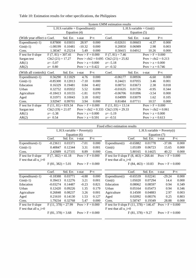
the restricted model consisting of equations (4)­(5) are reported in Table 10. The results

show that the income convergence is supported, even with the GMM estimation method.

The results in favor of the inequality convergence remain the same in Table 10. Parameter

β22 was always positive with statistical significance and its magnitude was much smaller

than unity, suggesting the inequality convergence in the Philippines, like the one found by

Benabou (1996) and Ravallion (2003).

The magnitudes of the positive effect of Expenditure and the negative effect of Gini

on Poverty are sensitive to specifications in the Philippines (Table 10), as in Thailand:

the coefficients are three to four times larger in equation (7) than in equation (6). This

again warns against the use of specification (6) when the dynamic effects from growth and

inequality on poverty are of concern. However, the difference in the magnitudes is smaller

in the Philippines than in Thailand. This is consistent with the contrast of the magnitudes

of parameter β33 in Tables 5 and 8. It is much larger in the Philippines than in Thailand,

indicating that poverty is more persistent in the Philippines than in Thailand. Because of

the persistence, the bias due to the use of specification (6) in place of specification (7) is

smaller in the Philippines.

When other measures of inequality and poverty were tried, qualitatively the same results

were obtained for the Philippines. Parameter β12 was estimated with a smaller standard error

when GE measures replaced Gini or FGT(1) poverty measure replaced Poverty, with more

statistical significance.

18

4.2 Simulating the Sources for Growth and Poverty Reduction

4.2.1 Simulation methods

Given the estimation results in the previous subsection, how much of the changes in growth

shown in Figures 1a and 2a and poverty reduction shown in Figures 1c and 2c can be

attributable to (i) initial differences in average consumption, poverty, and inequality; (ii)

differences in marginal impacts of the lagged values of average consumption, poverty, and

inequality (differences in β); and (iii) differences in the distribution of other controls Xt?

We simulate these sources for growth and poverty reduction by calculating counterfac­

tual dynamic paths of the two economies under several scenarios. Since our original micro

data cover different periods, we choose 1988 and 2000 as the comparison years (i.e., the two

years when we have micro data for both countries: see Figures 1 and 2). First, based on the

parameter estimates in Tables 5 and 8, we calculated the fitted values of residuals as follows:

ˆ ˆ α1j + ˆ �1jt, (8)ln yjt = β11 ln yj,t−1 + β12Ineq1,j,t−1 + β13Pov1,j,t−1 + Xj,t−1θ1 + ˆ η1t + ˆ

ˆ ˆ α2j + ˆ �2jt, (9)Ineq1jt = β21 ln yj,t−1 + β22Ineq1,j,t−1 + β23Pov1,j,t−1 + Xj,t−1θ2 + ˆ η2t + ˆ

ˆ ˆ α3j + ˆ �3jt.Pov1jt = β31 ln yj,t−1 + β32Ineq1,j,t−1 + β33Pov1,j,t−1 + Xj,t−1θ3 + ˆ η3t + ˆ (10)

For the first type of simulations (the impact of the initial differences), we give an

additional shock to one of the left­hand­side variables, say, the inequality, in 1988. Then

we sequentially solve the dynamic system until the year 2000, keeping the values of X, β,

θ, ˆ η, and ˆα, ˆ � constant. For the second type of simulations (the impact of the differences

in β), we give a counterfactual value to one of the parameters in β (say, replacing β12 for

the Philippines by β12 for Thailand) in 1988 and onwards. Then we sequentially solve the

dynamic system until the year 2000, keeping the values of X, θ, ˆ η, ˆα, ˆ �, and the other

parameters of β constant. For the third type of simulations (the impact of other controls),

we give counterfactual values to one of the variables in X (say, proportionally adjusting

Xeducation for the Philippines so that the Philippine educational achievement tracks that of

Thailand) in 1988 and onwards. Then we sequentially solve the dynamic system until the

year 2000, keeping the values of β, θ, ˆ η, ˆα, ˆ �, and the other variables of X constant.

4.2.2 Dynamic impacts of inequality

In this paper, we report the simulation results for the first and the second type, focusing on

the impacts of inequality on consequent growth and poverty reduction (Table 11). In the

19

first row, the baseline values that replicate the observed dynamic paths are reported. In the

Philippines, the annual growth rate of per­capita expenditure was 2.20% during the 1988­

2000 period, which was associated with the poverty reduction (in terms of headcount index)

at the annual rate of 0.27%. Both of these numbers are smaller than those of Thailand:

per­capita expenditure grew at 3.68% and the headcount poverty index declined at 1.40%

per annum during the 1988­2000 period. The baseline numbers clearly show the contrast

between the Philippines and Thailand.

In Simulation 1, we add a shock to equation (2) in 1988 so that the inequality level

in that year is halved from the actual value both in the Philippines and Thailand. The

reduction in Ineq1j,t−1 in the right­hand side of equations (1)­(3) increases growth rates

and decreases inequality and poverty in the next period. When the economy reaches the

year 2000, the cumulative effect on the growth of per­capita expenditures and on poverty

reduction is substantial. In the Philippines, the annual growth rate of per­capita expenditure

would have been much higher at 5.50% during the 1988­2000 period, which would have been

associated with a higher poverty reduction speed at 0.93%. Qualitatively the same change

would have occurred in Thailand: per­capita expenditure would have grown at 5.88% and

the headcount poverty index would have declined at 1.63% per annum during the 1988­2000

period.

An interesting finding is that the counterfactual performance under Simulation 1 is

very similar between Thailand and the Philippines. Although the estimate for β12 is larger in

Thailand than in the Philippines, implying that the marginal ill­effect of the lagged inequality

on growth is larger in Thailand, the simulation results show that the total, cumulative ill­

effect of the lagged inequality on growth is larger in the Philippines. This is because in

Simulation 1, we halved the initial inequality level in both countries. Since the inequality

level in year 1988 was much higher in the Philippines than in Thailand, the cumulative effect

of the counterfactual shock is much larger in the Philippines than in Thailand. Thus, we

obtain the results that the counterfactual performance under Simulation 1 is very similar

between Thailand and the Philippines. In other words, the high level of initial inequality was

one of the main contributors to slower growth and slower poverty reduction in the Philippines

than in Thailand.

In Simulation 2, we replace the value of β12 for the Philippines by that for Thailand,

and we replace the value of β12 for Thailand by that for the Philippines. As shown in Tables

5 and 8, the estimate for β12 is larger in Thailand than in the Philippines, implying that the

20

5

marginal ill­effect of the lagged inequality on growth is larger in Thailand. The simulation

results in Table 11 thus show the total, cumulative ill­effect of the lagged inequality on

growth due to the difference in marginal impacts of the lagged values of inequality between

the two countries.

The cumulative effect of this simulation on the growth of per­capita expenditures and

on poverty reduction is substantial when the economy reaches the year 2000. In the Philip­

pines, the annual growth rate of per­capita expenditure would have been negative (­1.49%)

during the 1988­2000 period, which would have been associated with an increase of poverty

at the annual rate of 0.47%. Thus the Philippine economy was very fortunate that its

value of β12 is lower than the value used in the counterfactual scenario corresponding to

Thailand’s. In sharp contrast, growth and poverty reduction would have been much acceler­

ated in Thailand if the economy would have had a lower value of β12 as in the Philippines:

per­capita expenditure would have grown at 9.79% and the headcount poverty index would

have declined at 2.58% per annum during the 1988­2000 period. With this rate of poverty

reduction, the headcount poverty index would have been zero in 2000 for the majority of

provinces in Thailand. In other words, the highly negative response of economic growth

to the lagged inequality was one of the main contributors to the slow poverty reduction in

Thailand (“slow” in relative to its phenomenal growth rate). The economic performance in

Thailand is often regarded as an case of less pro­poor growth associated with a substantial

economic growth, resulting in a reasonably high pace of poverty reduction (Kakwani et al.,

2004; Booth, 1997). Our analysis sheds new light on this phenomenon from the viewpoint

of dynamic relationship among growth, inequality, and poverty.

Conclusion

To empirically analyze the dynamics of, and relations among, growth, poverty, and inequal­

ity, this paper proposed a framework in which due attention is paid to the fact that the entire

distribution of per­capita real consumption changes over time and that empirical variables

of growth, poverty, and inequality are often compiled from the same micro dataset. Implica­

tions were derived from the framework, regarding the dynamic relationship among growth,

inequality, and poverty.

As an illustration, the dynamic model was applied to unique panel data of provinces

in the Philippines (1985­2003) and Thailand (1988­2002), which were compiled from micro

21

datasets of household expenditure surveys. The system GMM estimation results showed

that lagged levels of inequality reduce the speed of economic growth and poverty reduction

in Thailand directly and reduce the speed of economic growth directly and poverty reduction

indirectly in the Philippines. The magnitudes of the marginal effects of inequality were found

to be larger in Thailand than in the Philippines. It was also suggested that the fixed effect

estimation might underestimate the marginal effect of lagged inequality on subsequent in­

equality change and the marginal effect of lagged income on subsequent income. Our results

showed mixed evidence regarding the conditional income convergence among provinces but

clear evidence for the conditional inequality convergence in both countries. Regarding the

specification of the poverty determinants, our analysis suggested that the regression of cur­

rent poverty on current inequality and growth might overestimate the true dynamic effects

of growth and inequality on poverty reduction.

Simulation results based on the parameter estimates showed that the inequality factor,

which is due to differences in the initial inequality level and in its marginal impact between

the two countries, explained a substantial portion of the Philippine­Thai difference in eco­

nomic growth and poverty reduction during the late 1980s and 1990s. The comparison of

the two economies shed a new light on the understanding of a structural difference among

Asian countries. The mechanism underlying the difference in the initial inequality level and

in its marginal impact, however, still remains in the blackbox. Investigating the mechanism

utilizing micro data in these two countries is left for the next research agenda.

22

References

[1] Aghion, P., E. Caroli, and C. Garcia­Penalosa. 1999. “Inequality and Economic Growth: The Perspective of the New Growth Theories.” Journal of Economic Literature, vol.37, pp.1615­1660.

[2] Alesina, A. and D. Rodrik. 1994. “Distributive Politics and Economic Growth.”The Quarterly Journal of Economics, vol.109, issue 2, pp.465­490.

[3] Banerjee, A.V. and E. Duflo. 2003. “Inequality and Growth: What Can the Data Say?” Journal of Economic Growth, vol.8, No. 3, pp.267­299.

[4] Benabou, R. 1996. “Inequality and Growth. In B. Bernanke and J. Rotemberg (eds.) Na­tional Bureau of Economic Research Macroeconomics Annual. MIT Press, Cambridge, pp.11­74.

[5] Besley, T. and R. Burgess. 2003. “Halving Global Poverty.”Journal of Economic Per­spective, vol.17, No.3, pp.3­22.

[6] Blundell, R. and S. Bond. 1998. “Initial Conditions and Moment Restrictions in Dy­namic Panel Data Models.”Journal of Econometrics, vol.87, No.1, pp.115­143.

[7] Bond, S., A. Hoeffler, and J. Temple. 2001. “GMM Estimation of Empirical Growth Models.” C.E.P.R. Discussion Papers, No.3048.

[8] Booth, A. 1997. “Rapid Economic Growth and Poverty Decline: A comparison of In­donesia and Thailand 1981­1990,” Journal of International Development, vol.9, pp.169­187.

[9] Bourguignon, F. 2004. “The Poverty­Growth­Inequality Triangle.”Indian Council for Research on International Economic Relations.

[10] Datt, G. and M. Ravallion. 1992. “Growth and Redistribution Components of Changes in Poverty Measures: A Decomposition with Applications to Brazil and India in the 1980s.” Journal of Development Economics, vol.38, no.2, pp.275­295.

[11] Deininger, K. and L. Squire. 1998. “New ways of looking at old issues : inequality and growth.” The Journal of Development Economics, vol.57, pp.259­287.

[12] Fields, G. 2000. Distribution and Development, MIT press.

[13] Forbes, K. 2000. “A Reassessment of Relationship between Inequality and Growth.” American Economic Review, vol.90, No.4, pp.869­887.

[14] Foster, J.E. and A.K. Sen. 1997. “On Economic Inequality After a Quarter Century,” Annexe to A.K. Sen, On Economic Inequality, Enlarged Edition, Oxford: Clarendon Press, pp.107­219.

23

[15] Galor, O. and J. Zeira. 1993. “Income Distribution and Macroeconomics.” Review of Economic Studies, vol.60.

[16] Heltberg, R. 2004. “The Growth Elasticity of Poverty.” In Shorrocks and van der Hoeven (2004), pp.81­91.

[17] Jones, C.I. 2002. Introduction to Economic Growth. Second Edition, W.W. Norton and Company Inc.

[18] Kakwani, N. 1993. “Poverty and Economic Growth with Application to Cote D’Ivoire.” Review of Income and Wealth. vol.39, no.2, pp.121­139.

[19] Kakwani, N., S. Khandker, and H.H. Son. 2004. “Pro­poor Growth: Concepts and Mea­surement with Country Case Studies,” Working Paper 1, UNDP International Poverty Centre.

[20] Kakwani, N. and H.H. Son. 2006. “How Costly is it to Achieve the Millennium Devel­opment Goal of Halving Poverty between 1990 and 2015?” Working Paper 19, UNDP International Poverty Centre.

[21] Li, H. and H. Zou. 1998. “Income Inequality is not Harmful for Growth : Theory and Evidence.”Review of Development Economics, vol.2, no.3, pp.318­334.

[22] Perotti, R. 1996. “Growth, Income Distribution, and Democracy: What the Data Say.”Journal of Economic Growth,vol.1 June, pp.149­187.

[23] Quah, D. 2005. “Growth and Distribution,” mimeo. LSE. January 2005.

[24] Ravallion, M. 1998. “Does Aggregation Hide the Harmful Effects of Inequality on Growth?” Economics Letters, vol.61, no.1, pp.73­77.

[25] —–. 2003. “Inequality Convergence.” Economics Letters, vol.80, pp.351­356.

[26] —–. 2004. “Looking Beyond Averages.” In Shorrocks and van der Hoeven (2004), pp.62­80.

[27] Sawada, Y. 2004. “An Assessment of Philippine Performance in Reducing Poverty By Using the Millennium Development Goals as the Benchmark.” A background paper for the Philippines Poverty Assessment, the World Bank.

[28] Shorrocks, Anthony F. and Rolph van der Hoeven (eds.). 2004. Growth, Inequality, and Poverty: Prospects for Pro­Poor Economic Development. Oxford: Oxford University Press.

[29] World Bank. 1993. The East Asian Miracle: Economic Growth and Public Policy. Ox­ford University Press.

[30] —–. 2004. World Development Indicators, the World Bank.

24

Figure 1a: Time Series of Expenditure , Thailand

8.5

8

7.5

7

6.5

6

1988 1990 1992 1994 1996 1998 2000 2002

Figure 1b: Time Series of Gini , Thailand

0.5

0.4

0.3

0.2

0.1 1988 1990 1992 1994 1996 1998 2000 2002

Figure 1c: Time Series of Poverty , Thailand

0.6

0.5

0.4

0.3

0.2

0.1

0 1988 1990 1992 1994 1996 1998 2000 2002

National mean Mean across provinces Max Min

Figure 2a: Time Series of Expenditure , the Philippines

11.5

11

10.5

10

9.5

9

8.5

8

7.5 1985 1988 1991 1994 1997 2000 2003

Figure 2b: Time Series of Gini , the Philippines

0.6

0.5

0.4

0.3

0.2

0.1 1985 1988 1991 1994 1997 2000 2003

Figure 2c: Time Series of Poverty , the Philippines

1

0.8

0.6

0.4

0.2

0 1985 1988 1991 1994 1997 2000 2003

National mean Mean across provinces Max Min

Table 1: Summary statistics of regression variables, Thailand

Variable Definition Obs Mean Std. Dev. Min Max Expenditure Log mean per-capita consumption in each province in real Bahts. 599 7.0745 0.3322 6.2074 8.0794 Gini Gini coefficient of per-capita consumption in each province. 599 0.3331 0.0442 0.2243 0.4701 Poverty Head count index in each province based on per-capita consumption. 540 0.1071 0.1140 0.0000 0.5627 Education Ratio of households whose head has tertiary education (more than 12 years of schooling). 599 0.0748 0.0488 0.0018 0.3566 Urban Ratio of households who live in urban areas. 599 0.8772 0.1427 0.0000 1.0000 Agriculture Ratio of households whose head is engaged in agriculture. 599 0.5372 0.1976 0.0074 0.9608 Aged Population share of individuals aged more than or equal to 65. 599 0.1543 0.0563 0.0000 0.3424

Table 2: Summary statistics of regression variables, the Philippines

Variable Definition Obs Mean Std. Dev. Min Max Expenditure Log mean per-capita consumption in each province in real Pesos. 556 9.1725 0.6122 7.7646 10.7446 Gini Gini coefficient of per-capita consumption in each province. 556 0.3595 0.0516 0.2005 0.5165 Poverty Head count index in each province based on per-capita consumption. 556 0.4984 0.1815 0.0469 0.9071 Education Ratio of households whose head has tertiary education (more than 10 years of schooling). 556 0.1522 0.0690 0.0138 0.4055 Urban Ratio of households who live in urban areas. 556 0.3493 0.2242 0.0387 1.0000 Agriculture Ratio of households whose head is engaged in agriculture. 556 0.3705 0.1509 0.1000 0.7892 Aged Population share of individuals aged more than or equal to 65. 556 0.1304 0.0558 0.0000 0.3538

Table 3: Bi-variate correlation coefficients of mean per-capita consumption expenditure, inequality measures, and poverty measures in Thailand

Expenditur e FGT(0) FGT(1) FGT(2) Watt's

Index

Clark-Watt's

Index (-1) GE(-1) GE(0) GE(1) GE(2) Gini

Expenditure 1.0000 FGT(0) -0.7570 1.0000 FGT(1) -0.6746 0.9550 1.0000 FGT(2) -0.5991 0.8886 0.9817 1.0000 Watt's Index -0.6626 0.9454 0.9994 0.9879 1.0000 Clark-Watt's Index (-1) -0.6482 0.9333 0.9970 0.9934 0.9992 1.0000 GE(-1) -0.0572 0.3541 0.3684 0.3606 0.3681 0.3673 1.0000 GE(0) -0.1831 0.4346 0.4264 0.4017 0.4232 0.4190 0.9796 1.0000 GE(1) -0.3149 0.5081 0.4771 0.4351 0.4707 0.4630 0.9084 0.9725 1.0000 GE(2) -0.4226 0.5586 0.5082 0.4514 0.4991 0.4883 0.7753 0.8773 0.9628 1.0000 Gini -0.1769 0.4101 0.3930 0.3630 0.3887 0.3833 0.9677 0.9921 0.9634 0.8627 1.0000

Table 4: Bi-variate correlation coefficients of mean per-capita consumption expenditure, inequality measures, and poverty measures in the Philippines

Expenditur e FGT(0) FGT(1) FGT(2) Watt's

Index

Clark-Watt's

Index (-1) GE(-1) GE(0) GE(1) GE(2) Gini

Expenditure 1.0000 FGT(0) -0.7332 1.0000 FGT(1) -0.6643 0.9539 1.0000 FGT(2) -0.6100 0.8926 0.9855 1.0000 Watt's Index -0.6360 0.9209 0.9910 0.9915 1.0000 Clark-Watt's Index (-1) -0.5983 0.8771 0.9742 0.9928 0.9935 1.0000 GE(-1) 0.1268 -0.0418 0.0384 0.0764 0.0740 0.0959 1.0000 GE(0) 0.0626 0.0564 0.1221 0.1481 0.1525 0.1662 0.9786 1.0000 GE(1) -0.0263 0.1602 0.2067 0.2188 0.2282 0.2327 0.8968 0.9648 1.0000 GE(2) -0.1070 0.2121 0.2378 0.2381 0.2476 0.2446 0.6799 0.7844 0.9098 1.0000 Gini 0.0797 0.0383 0.1046 0.1317 0.1365 0.1505 0.9669 0.9919 0.9502 0.7553 1.0000

Table 5: System-GMM estimation results, Thailand

L.H.S.variable = Expenditure(t) L.H.S.variable = Gini(t) L.H.S.variable = Poverty(t) Equation (1) Equation (2) Equation (3)

(With year effect only) Coef. Std. Err. t-stat P>t Coef. Std. Err. t-stat P>t Coef. Std. Err. t-stat P>t Expenditure(t-1) 0.94495 0.04833 19.55 0.000 -0.08528 0.01598 -5.34 0.000 -0.06095 0.03055 -1.99 0.050 Gini(t-1) -2.15308 0.24125 -8.92 0.000 0.40460 0.07464 5.42 0.000 0.24499 0.10154 2.41 0.018 Poverty(t-1) 0.87875 0.18378 4.78 0.000 -0.14477 0.04538 -3.19 0.002 0.21302 0.11883 1.79 0.077 Cons. 1.12485 0.33858 3.32 0.001 0.82445 0.10155 8.12 0.000 0.39707 0.20482 1.94 0.056 F test for 0 slope F (9, 75) = 124.10 Prov > F = 0.000 F (9, 75) = 9.49 Prov > F = 0.002 F (9, 75) = 38.18 Prov > F = 0.000 Sargan test Chi2 (28) = 41.22 Prov > chi2 = 0.051 Chi2 (28) = 34.80 Prov > chi2 = 0.176 Chi2 (28) = 45.48 Prov > chi2 = 0.020 AR(1) z= -5.99 Prov > z = 0.000 z= -5.80 Prov > z = 0.000 z= -4.74 Prov > z = 0.000 AR(2) z= -0.52 Prov > z = 0.603 z= -0.58 Prov > z = 0.563 z= -0.08 Prov > z = 0.934

(With year effect and controls) Coef. Std. Err. t-stat P>t Coef. Std. Err. t-stat P>t Coef. Std. Err. t-stat P>t Expenditure(t-1) 0.84056 0.11925 7.05 0.000 -0.09932 0.02227 -4.46 0.000 -0.03217 0.03699 -0.87 0.387 Gini(t-1) -1.86693 0.29137 -6.41 0.000 0.42685 0.08256 5.17 0.000 0.19579 0.11061 1.77 0.081 Poverty(t-1) 0.80694 0.22470 3.59 0.001 -0.16907 0.04554 -3.71 0.000 0.19292 0.12471 1.55 0.126 Education -0.81477 0.34413 -2.37 0.020 -0.08046 0.06159 -1.31 0.195 0.06082 0.10668 0.57 0.570 Urban -0.01926 0.12551 -0.15 0.878 -0.03910 0.02457 -1.59 0.116 -0.06022 0.05172 -1.16 0.248 Agriculture -0.25471 0.09573 -2.66 0.010 -0.00994 0.01955 -0.51 0.613 0.11710 0.02600 4.50 0.000 Aged -0.05058 0.18204 -0.28 0.782 -0.15426 0.03639 -4.24 0.000 -0.10336 0.07640 -1.35 0.180 Cons. 1.99680 0.85970 2.32 0.023 0.98702 0.16056 6.15 0.000 0.21238 0.27813 0.76 0.448 F test for 0 slope F (13, 75) = 49.09 Prov > F = 0.000 F (13, 75) = 8.61 Prov > F = 0.000 F (13, 75) = 26.71 Prov > F = 0.000 Sargan test Chi2 (26) = 30.70 Prov > chi2 = 0.240 Chi2 (26) =32.92 Prov > chi2 = 0.164 Chi2 (26) = 45.99 Prov > chi2 = 0.009 AR(1) z= -5.77 Prov > z = 0.000 z= -5.67 Prov > z = 0.000 z= -4.83 Prov > z = 0.000 AR(2) z= -0.69 Prov > z = 0.489 z= -0.27 Prov > z = 0.787 z= -0.10 Prov > z = 0.923

Note: The number of observations is 437 and the number of groups in the panel is 75.

Table 6: Results under different estimation methods, Thailand

L.H.S.variable = Expenditure(t) L.H.S.variable = Gini(t) L.H.S.variable = Poverty(t) Equation (1) Equation (2) Equation (3)

1. Pooled OLS

(With year effect only) Coef. Std. Err. t-stat P>t Coef. Std. Err. t-stat P>t Coef. Std. Err. t-stat P>t Expenditure(t-1) 0.86076 0.03882 22.17 0.000 -0.03698 0.00756 -4.89 0.000 -0.08383 0.01582 -5.30 0.000 Gini(t-1) -1.38502 0.20161 -6.87 0.000 0.35707 0.04384 8.14 0.000 0.25856 0.08264 3.13 0.002 Poverty(t-1) 0.30309 0.12471 2.43 0.015 -0.00360 0.02643 -0.14 0.892 0.31479 0.06573 4.79 0.000

(With year effect and controls) Coef. Std. Err. t-stat P>t Coef. Std. Err. t-stat P>t Coef. Std. Err. t-stat P>t Expenditure(t-1) 0.62897 0.08169 7.70 0.000 -0.04903 0.01530 -3.20 0.001 -0.10346 0.02863 -3.61 0.000 Gini(t-1) -1.11172 0.22511 -4.94 0.000 0.36897 0.04686 7.87 0.000 0.26252 0.09119 2.88 0.004 Poverty(t-1) 0.14230 0.14520 0.98 0.328 -0.03249 0.03015 -1.08 0.282 0.24190 0.07141 3.39 0.001

2. Fixed effects

(With year effect only) Coef. Std. Err. t-stat P>t Coef. Std. Err. t-stat P>t Coef. Std. Err. t-stat P>t Expenditure(t-1) 0.20567 0.05777 3.56 0.000 -0.01840 0.01470 -1.25 0.211 0.01558 0.02451 0.64 0.525 Gini(t-1) -0.53511 0.20691 -2.59 0.010 0.04126 0.05267 0.78 0.434 0.05839 0.08778 0.67 0.506 Poverty(t-1) 0.00316 0.12041 0.03 0.979 -0.00358 0.03065 -0.12 0.907 0.09471 0.05108 1.85 0.064

(With year effect and controls) Coef. Std. Err. t-stat P>t Coef. Std. Err. t-stat P>t Coef. Std. Err. t-stat P>t Expenditure(t-1) 0.19813 0.07006 2.83 0.005 -0.01719 0.01778 -0.97 0.334 -0.01798 0.02955 -0.61 0.543 Gini(t-1) -0.55029 0.21024 -2.62 0.009 0.05221 0.05336 0.98 0.328 0.10722 0.08867 1.21 0.227 Poverty(t-1) 0.02936 0.12849 0.23 0.819 -0.00913 0.03261 -0.28 0.780 0.04123 0.05419 0.76 0.447

Note: Parameter estimates for other right-hand-side variables and test results are deleted for brevity. Full results as those in Table 5 are available on request.

Table 7: Estimation results for other specifications, Thailand

System GMM estimation results L.H.S.variable = Expenditure(t) L.H.S.variable = Gini(t)

Equation (4) Equation (5)

(With year effect on Coef. Std. Err. t-stat P>t Coef. Std. Err. t-stat P>t Expenditure(t-1) 0.74231 0.04418 16.80 0.000 -0.04624 0.00710 -6.51 0.000 Gini(t-1) -1.55987 0.19409 -8.04 0.000 0.28515 0.04876 5.85 0.000 Cons. 2.45819 0.31788 7.73 0.000 0.57265 0.05196 11.02 0.000 F test for 0 slope F (8, 75) = 108.63 Prov > F = 0.000 F (8, 75) = 16.06 Prov > F = 0.000 Sargan test Chi2 (28) = 38.21 Prov > chi2 = 0.094 Chi2 (28) = 34.46 Prov > chi2 = 0.380 AR(1) z= -5.59 Prov > z = 0.000 z= -5.72 Prov > z = 0.000 AR(2) z= -0.03 Prov > z = 0.980 z= -0.16 Prov > z = 0.875

(With all controls) Coef. Std. Err. t-stat P>t Coef. Std. Err. t-stat P>t Expenditure(t-1) 0.51830 0.08932 5.80 0.000 -0.04070 0.01133 -3.59 0.001 Gini(t-1) -1.27729 0.19169 -6.66 0.000 0.29248 0.05409 5.41 0.000 Education -0.35277 0.35138 -1.00 0.319 -0.14409 0.06478 -2.22 0.029 Urban -0.08967 0.12535 -0.72 0.477 -0.02231 0.02129 -1.05 0.298 Agriculture -0.31745 0.09333 -3.40 0.001 -0.00346 0.01817 -0.19 0.850 Aged -0.17895 0.18427 -0.97 0.335 -0.12567 0.03748 -3.35 0.001 Cons. 4.24711 0.63730 6.66 0.000 0.58144 0.08678 6.70 0.000 F test for 0 slope F (12, 75) = 52.82 Prov > F = 0.000 F (12, 75) = 12.85 Prov > F = 0.000 Sargan test Chi2 (26) = 32.84 Prov > chi2 = 0.167 Chi2 (26) = 33.29 Prov > chi2 = 0.154 AR(1) z= -5.57 Prov > z = 0.000 z= -5.73 Prov > z = 0.000 AR(2) z= -0.19 Prov > z = 0.847 z= 0.21 Prov > z = 0.836

Fixed effect estimation results L.H.S.variable = Poverty(t) L.H.S.variable = Poverty(t)

Equation (6) Equation (7) Coef. Std. Err. t-stat P>t Coef. Std. Err. t-stat P>t

Expenditure(t-1) -0.01350 0.01888 -0.72 0.475 Expenditure(t) -0.30138 0.01627 -18.52 0.000 Gini(t-1) 0.13247 0.07838 1.69 0.092 Gini(t) 0.75709 0.06681 11.33 0.000 Cons. 0.13107 0.12603 1.04 0.299 Cons. 1.97931 0.10721 18.46 0.000 F test for 0 slope F test that all u_i=0

F (8, 439)

F (75, 439)

= 24.03

= 3.67

Prov > F

Prov > F

= 0.000

= 0.000

F test for 0 slope F test that all u_

F (9, 514) i=0

F (75, 514

= 124.75

) = 3.85

Prov > F = 0.000

Prov > F = 0.000

Coef. Std. Err. t-stat P>t Coef. Std. Err. t-stat P>t Expenditure(t-1) -0.03303 0.02194 -1.51 0.133 Expenditure(t) -0.35668 0.01810 -19.70 0.000 Gini(t-1) 0.13858 0.07847 1.77 0.078 Gini(t) 0.70479 0.06360 11.08 0.000 Education 0.13573 0.11105 1.22 0.222 Education 0.59290 0.08656 6.85 0.000 Urban -0.15578 0.06471 -2.41 0.016 Urban -0.02288 0.03948 -0.58 0.563 Agriculture 0.04838 0.03676 1.32 0.189 Agriculture -0.00234 0.03058 -0.08 0.939 Aged -0.10540 0.06730 -1.57 0.118 Aged -0.15524 0.05449 -2.85 0.005 Cons. 0.38321 0.16962 2.26 0.024 Cons. 2.38537 0.13418 17.78 0.000 F test for 0 slope F (12, 435) = 17.49 Prov > F = 0.000 F test for 0 slope F (13, 510) = 102.89 Prov > F = 0.000 F test that all u_i=0 F test that all u_i=0

F (75, 435) = 3.15 Prov > F = 0.000 F (75, 510) = 2.48 Prov > F = 0.000

Table 8: System-GMM estimation results, the Philippines

L.H.S.variable = Expenditure(t) L.H.S.variable = Gini(t) L.H.S.variable = Poverty(t) Equation (1) Equation (2) Equation (3)

(With year effect only) Coef. Std. Err. t-stat P>t Coef. Std. Err. t-stat P>t Coef. Std. Err. t-stat P>t Expenditure(t-1) 1.55836 0.09266 16.82 0.000 -0.06690 0.02344 -2.85 0.005 -0.06109 0.05936 -1.03 0.307 Gini(t-1) -1.85169 0.37447 -4.94 0.000 0.32009 0.09194 3.48 0.001 0.02098 0.12011 0.17 0.862 Poverty(t-1) 1.22731 0.15771 7.78 0.000 -0.08046 0.03984 -2.02 0.047 0.64946 0.11223 5.79 0.000 Cons. -4.82464 0.80716 -5.98 0.000 0.85617 0.20982 4.08 0.000 0.71298 0.55572 1.28 0.203 F test for 0 slope F (8, 81) = 143.94 Prov > F = 0.000 F (8, 81) = 7.73 Prov > F = 0.000 F (8, 81) = 75.16 Prov > F = 0.000 Sargan test Chi2 (21) = 17.79 Prov > chi2 = 0.662 Chi2 (21) = 24.92 Prov > chi2 = 0.251 Chi2 (21) = 35.27 Prov > chi2 = 0.026 AR(1) z= -4.65 Prov > z = 0.000 z= -5.10 Prov > z = 0.000 z= -5.81 Prov > z = 0.000 AR(2) z= 1.32 Prov > z = 0.188 z= -0.42 Prov > z = 0.672 z= 0.82 Prov > z = 0.411

(With year effect and controls) Coef. Std. Err. t-stat P>t Coef. Std. Err. t-stat P>t Coef. Std. Err. t-stat P>t Expenditure(t-1) 1.11018 0.09195 12.07 0.000 -0.05712 0.02145 -2.66 0.009 -0.04026 0.03898 -1.03 0.305 Gini(t-1) -1.53444 0.30550 -5.02 0.000 0.26171 0.09013 2.90 0.005 0.06899 0.12062 0.57 0.569 Poverty(t-1) 0.73428 0.10762 6.82 0.000 -0.01029 0.03233 -0.32 0.751 0.38904 0.09272 4.20 0.000 Education -0.18135 0.25189 -0.72 0.474 0.04823 0.07855 0.61 0.541 0.00512 0.15067 0.03 0.973 Urban 0.20316 0.06920 2.94 0.004 -0.01164 0.02340 -0.50 0.620 -0.17736 0.04540 -3.91 0.000 Agriculture 0.26320 0.12791 2.06 0.043 0.09280 0.03239 2.86 0.005 -0.18729 0.07839 -2.39 0.019 Aged 0.54262 0.20358 2.67 0.009 0.08505 0.06816 1.25 0.216 -0.21626 0.15801 -1.37 0.175 Cons. -0.74383 0.72821 -1.02 0.310 0.69240 0.18866 3.67 0.000 0.70082 0.35738 1.96 0.053 F test for 0 slope F (12, 81) = 720.34 Prov > F = 0.000 F (12, 81) = 12.13 Prov > F = 0.000 F (12, 81) = 78.00 Prov > F = 0.000 Sargan test Chi2 (19) = 21.46 Prov > chi2 = 0.312 Chi2 (9) = 29.37 Prov > chi2 = 0.060 Chi2 (19) = 25.77 Prov > chi2 = 0.137 AR(1) z= -4.92 Prov > z = 0.000 z= -5.06 Prov > z = 0.000 z= -4.96 Prov > z = 0.000 AR(2) z= 0.49 Prov > z = 0.622 z= -0.51 Prov > z = 0.610 z= 0.09 Prov > z = 0.926

Note: The number of observations is 388 and the number of groups in the panel is 82.

Table 9: Results under different estimation methods, the Philippines

L.H.S.variable = Expenditure(t) L.H.S.variable = Gini(t) L.H.S.variable = Poverty(t) Equation (1) Equation (2) Equation (3)

1. Pooled OLS

(With year effect only) Coef. Std. Err. t-stat P>t Coef. Std. Err. t-stat P>t Coef. Std. Err. t-stat P>t Expenditure(t-1) 0.97038 0.05180 18.73 0.000 -0.04805 0.01503 -3.20 0.001 -0.14373 0.03761 -3.82 0.000 Gini(t-1) -0.52827 0.17169 -3.08 0.002 0.60846 0.05220 11.66 0.000 0.06335 0.10625 0.60 0.551 Poverty(t-1) 0.09813 0.09990 0.98 0.326 -0.05999 0.02981 -2.01 0.045 0.61854 0.07300 8.47 0.000

(With year effect and controls) Coef. Std. Err. t-stat P>t Coef. Std. Err. t-stat P>t Coef. Std. Err. t-stat P>t Expenditure(t-1) 0.81028 0.05808 13.95 0.000 -0.06615 0.01755 -3.77 0.000 -0.06690 0.04052 -1.65 0.099 Gini(t-1) -0.64029 0.16232 -3.94 0.000 0.58424 0.05042 11.59 0.000 0.13389 0.10441 1.28 0.200 Poverty(t-1) 0.22762 0.10062 2.26 0.024 -0.04699 0.03024 -1.55 0.121 0.53135 0.07376 7.20 0.000

2. Fixed effects

(With year effect only) Coef. Std. Err. t-stat P>t Coef. Std. Err. t-stat P>t Coef. Std. Err. t-stat P>t Expenditure(t-1) 0.27426 0.10007 2.74 0.006 0.00752 0.02811 0.27 0.789 -0.15788 0.06670 -2.37 0.018 Gini(t-1) -0.45653 0.22927 -1.99 0.047 -0.02668 0.06441 -0.41 0.679 0.28581 0.15282 1.87 0.062 Poverty(t-1) -0.01482 0.12896 -0.11 0.909 0.02072 0.03623 0.57 0.568 0.11678 0.08596 1.36 0.175

(With year effect and controls) Coef. Std. Err. t-stat P>t Coef. Std. Err. t-stat P>t Coef. Std. Err. t-stat P>t Expenditure(t-1) 0.22017 0.10160 2.17 0.031 -0.00698 0.02868 -0.24 0.808 -0.13242 0.06755 -1.96 0.051 Gini(t-1) -0.50061 0.22802 -2.20 0.029 -0.03457 0.06437 -0.54 0.592 0.31245 0.15161 2.06 0.040 Poverty(t-1) 0.01561 0.12950 0.12 0.904 0.02332 0.03656 0.64 0.524 0.07907 0.08610 0.92 0.359

Note: Parameter estimates for other right-hand-side variables and test results are deleted for brevity. Full results as those in Table 8 are available on request.

Table 10: Estimation results for other specifications, the Philippines

System GMM estimation results L.H.S.variable = Expenditure(t) L.H.S.variable = Gini(t)

Equation (4) Equation (5)

(With year effect on Coef. Std. Err. t-stat P>t Coef. Std. Err. t-stat P>t Expenditure(t-1) 0.87800 0.03031 28.97 0.000 -0.02631 0.00603 -4.37 0.000 Gini(t-1) -1.08199 0.10481 -10.32 0.000 0.20850 0.06989 2.98 0.003 Cons. 1.38347 0.25214 5.49 0.000 0.50415 0.04912 10.26 0.000 F test for 0 slope F (7, 81) = 307.41 Prov > F = 0.000 F (7, 81) = 7.46 Prov > F = 0.000 Sargan test Chi2 (21) = 17.27 Prov > chi2 = 0.695 Chi2 (21) = 25.82 Prov > chi2 = 0.213 AR(1) z= -5.07 Prov > z = 0.000 z= -5.18 Prov > z = 0.000 AR(2) z= 0.80 Prov > z = 0.422 z= -0.32 Prov > z = 0.746

(With all controls) Coef. Std. Err. t-stat P>t Coef. Std. Err. t-stat P>t Expenditure(t-1) 0.56290 0.11829 4.76 0.000 -0.06177 0.00936 -6.60 0.000 Gini(t-1) -0.85300 0.12013 -7.10 0.000 0.24421 0.07055 3.46 0.001 Education 0.16329 0.19481 0.84 0.402 0.08751 0.03673 2.38 0.018 Urban 0.32752 0.05932 5.52 0.000 -0.01635 0.01726 -0.95 0.344 Agriculture -0.18413 0.10155 -1.81 0.070 -0.06706 0.01896 -3.54 0.000 Aged 0.31971 0.10043 3.18 0.002 0.04999 0.03079 1.62 0.105 Cons. 3.92947 0.99701 3.94 0.000 0.81484 0.07711 10.57 0.000 F test for 0 slope F (11, 81) = 819.34 Prov > F = 0.000 F (11, 81) = 13.14 Prov > F = 0.000 Sargan test Chi2 (19) = 21.07 Prov > chi2 = 0.333 Chi2 (19) = 29.33 Prov > chi2 = 0.061 AR(1) z= -5.38 Prov > z = 0.000 z= -5.19 Prov > z = 0.000 AR(2) z= 0.54 Prov > z = 0.591 z= -0.51 Prov > z = 0.613

Fixed effect estimation results L.H.S.variable = Poverty(t) L.H.S.variable = Poverty(t)

Equation (6) Equation (7) Coef. Std. Err. t-stat P>t Coef. Std. Err. t-stat P>t

Expenditure(t-1) -0.23611 0.03371 -7.01 0.000 Expenditure(t) -0.65882 0.01778 -37.06 0.000 Gini(t-1) 0.40847 0.12344 3.31 0.001 Gini(t) 1.05189 0.06723 15.65 0.000 Cons. 2.42889 0.27335 8.89 0.000 Cons. 5.80165 0.14425 40.22 0.000 F test for 0 slope F (7, 382) = 41.18 Prov > F = 0.000 F test for 0 slope F (8, 463) = 268.44 Prov > F = 0.000 F test that all u_i=0 F test that all u_i=0

F (81, 382) = 5.01 Prov > F = 0.000 F (84, 463) = 10.83 Prov > F = 0.000

Coef. Std. Err. t-stat P>t Coef. Std. Err. t-stat P>t Expenditure(t-1) -0.18388 0.03771 -4.88 0.000 Expenditure(t) -0.65539 0.02241 -29.24 0.000 Gini(t-1) 0.39413 0.12276 3.21 0.001 Gini(t) 1.05020 0.07294 14.4 0.000 Education -0.03274 0.14487 -0.23 0.821 Education 0.08062 0.08597 0.94 0.349 Urban 0.12420 0.09226 1.35 0.179 Urban 0.05164 0.05473 0.94 0.346 Agriculture 0.26848 0.08237 3.26 0.001 Agriculture 0.14500 0.04883 2.97 0.003 Aged 0.21610 0.14130 1.53 0.127 Aged 0.02092 0.08376 0.25 0.803 Cons. 1.79234 0.32768 5.47 0.000 Cons. 5.58747 0.19349 28.88 0.000 F test for 0 slope F (11, 378) = 27.99 Prov > F = 0.000 F test for 0 slope F (11, 378) = 146.47 Prov > F = 0.000 F test that all u_i=0 F test that all u_i=0

F (81, 378) = 3.68 Prov > F = 0.000 F (81, 378) = 9.27 Prov > F = 0.000

Table 11: Simulation results for the dynamic impacts of inequality, 1988-2000

The Philippines Thailand Annual growth Annual rate of Annual growth Annual rate of rate of per-capita poverty rate of per-capita poverty expenditure (%) reduction (%) expenditure (%) reduction (%)

Baseline 2.20 0.27 3.68 1.40 Simulation 1: Adding a shock to equation (2) in 1988 so that the inequality level in that year is halved from the actual value

Counterfactual 5.50 0.93 5.88 1.63 Simulation 2: Replacing the value of β12 (the marginal effect of the lagged inequality on growth) by the value of the other country

Counterfactual -1.49 -0.47 9.79 2.58