37

Dynami s of PDE, Vol.6, No.3, 253-289, 2009Expli it multipeakon solutions of Novikov's ubi allynonlinear integrable CamassaHolm type equationAndrew N. W. Hone, Hans Lundmark, and Ja ek SzmigielskiCommuni ated by Mark Ablowitz, re eived May 27, 2009.Abstra t. Re ently Vladimir Novikov found a new integrable analogue ofthe CamassaHolm equation whi h has nonlinear terms that are ubi , ratherthan quadrati , and whi h admits peaked soliton solutions (peakons). In thispaper, the expli it formulas for multipeakon solutions of Novikov's ubi allynonlinear equation are al ulated, using the matrix Lax pair found by Honeand Wang. By a transformation of Liouville type, the asso iated spe tralproblem is related to a ubi string equation, whi h is dual to the ubi stringthat was previously found in the work of Lundmark and Szmigielski on themultipeakons of the DegasperisPro esi equation.Contents1. Introdu tion 2542. Ba kground 2553. Novikov's equation 2564. Forward spe tral problem 2575. The dual ubi string 2626. Relation to the Neumann-like ubi string 2657. Inverse spe tral problem 2668. Evaluation of bimoment determinants 2699. The multipeakon solution 271Appendix A. Combinatorial results 274Appendix B. Veri ation of the Lax pair for peakons 283Referen es 2872000 Mathemati s Subje t Classi ation. Primary 37K15.Key words and phrases. Peakons, ubi string, Novikov's equation, DegasperisPro esi equa-tion, distributional Lax pair, sum of minors.HL is supported by the Swedish Resear h Coun il (Vetenskapsrådet), and JS by the Na-tional S ien es and Engineering Resear h Coun il of Canada (NSERC). HL and JS would liketo a knowledge the hospitality of the Mathemati al Resear h and Conferen e Center, Bdlewo,Poland, and the Department of Mathemati s and Statisti s, University of Saskat hewan, Canada. ©2009 International Press253

254 ANDREW N. W. HONE, HANS LUNDMARK, AND JACEK SZMIGIELSKI1. Introdu tionIntegrable PDEs with nonsmooth solutions have attra ted mu h attention inre ent years, sin e the dis overy of the CamassaHolm shallow water wave equa-tion and its peak-shaped soliton solutions alled peakons [9. Another equationwith similar properties is the DegasperisPro esi equation [19, 18. Our purposein this paper is to expli itly ompute the multipeakon solutions of a new inte-grable PDE, equation (3.1) below, whi h is of the CamassaHolm form ut −uxxt =F (u, ux, uxx, . . . ), but has ubi ally nonlinear terms instead of quadrati . Thisequation was found by Vladimir Novikov [48, and rst published in a re ent paperby Hone and Wang [32.There are several reasons why peakons are interesting. In water wave theory,the CamassaHolm and DegasperisPro esi equations ombine two desired features,namely soliton intera tions and wave breaking [13, and the peakons are also remi-nis ent of Stokes waves peaked waves of largest amplitude that are exa t solutionsof the governing equations for water waves [50, 12, 14. (See [34, 15 for moreinformation about the role of these equations in water wave theory.) They are alsointeresting from the point of view of general analysis of PDEs, sin e they providemany subtle and hallenging problems on erning existen e, uniqueness, stabilityand breakdown of solutions. (The literature on this is too large to be surveyedhere, but we will mention a few referen es relevant to our work in due ourse.)In studying su h questions, it is useful to have a ess to expli it exa t solutions,and this is provided by peakons. In addition, the mathemati s of peakons is verybeautiful in itself, with onne tions to lassi al topi s su h as SturmLiouville the-ory, orthogonal polynomials, and ontinued fra tions of Stieltjes type [1, 2, andgeneralizations thereof [43, 44, 37, 3, 5.We also mention the important fa t that peakons are orbitally stable, in thesense that a solution that initially is lose to a peakon solution is also lose tosome peakon solution at a later time; see [17, 21, 39 for pre ise results on erningCamassaHolm peakons, and [40 for the DegasperisPro esi ase.The n-peakon solution of Novikov's equation will be omputed by inverse spe -tral methods. The spatial equation in the Lax pair for Novikov's equation turns outto be equivalent to what we all the dual ubi string, a spe tral problem loselyrelated to the ubi string that was used for nding the multipeakon solutions tothe DegasperisPro esi equation [43, 44, 37. On e this relation is established,the Novikov peakon solution an be derived in a straightforward way using the re-sults obtained in [37. The onstants of motion have a more ompli ated stru turethan in the CamassaHolm and DegasperisPro esi ases, and the study of thisgives as an interesting by-produ t a ombinatorial identity on erning the sum ofall minors in a symmetri matrix, whi h we have dubbed the Canada Day Theorem(Theorem 4.1, proved in Appendix A).The peakon problem for Novikov's equation presents in addition one important hallenge. Unlike its CamassaHolm or DegasperisPro esi ounterparts, the Laxpair for the Novikov equation is originally ill-dened in the peakon se tor. Theproblem is aused by terms whi h involve multipli ation of a singular measure by adis ontinuous fun tion. We prove in Appendix B that there exists a regularizationof the Lax pair whi h preserves integrability of the peakon se tor, thus allowing usto use spe tral and inverse spe tral methods to obtain the multipeakon solutions tothe Novikov equation. This regularization problem has a subtle but nevertheless real

EXPLICIT MULTIPEAKON SOLUTIONS OF NOVIKOV'S EQUATION 255impa t on the formulas. In general, the use of Lax pairs to onstru t distributionalsolutions to nonlinear equations whi h are Lax integrable in the smooth se tor butmay not be so in the whole non-smooth se tor is relatively un harted territory, andthe ase of Novikov's equation may provide some relevant insight in this regard.2. Ba kgroundThe main example of a PDE admitting peaked solitons is the family(2.1) ut − uxxt + (b + 1)uux = buxuxx + uuxxx,often written as(2.2) mt +mxu+ bmux = 0, m = u− uxx,whi h was introdu ed by Degasperis, Holm and Hone [18, and is Hamiltonian forall values of b [28. It in ludes the CamassaHolm equation as the ase b = 2,and another integrable PDE alled the DegasperisPro esi equation [19, 18 as the ase b = 3. These are the only values of b for whi h the equation is integrable,a ording to a variety of integrability tests [19, 46, 31, 33. (However, we notethat the ase b = 0 is ex luded from the aforementioned integrability tests; yet this ase provides a regularization of the invis id Burgers equation that is Hamiltonianand has lassi al solutions globally in time [6. See also [29, 30 for studies of (2.1)for various values of b.) Multipeakons are weak solutions of the form(2.3) u(x, t) =
n∑
i=1
mi(t) e−|x−xi(t)|,formed through superposition of n peakons (peaked solitons of the shape e−|x|).This ansatz satises the PDE (2.2) if and only if the positions (x1, . . . , xn) andmomenta (m1, . . . ,mn) of the peakons obey the following system of 2n ODEs:(2.4) xk =
n∑
i=1
mi e−|xk−xi|, mk = (b− 1)mk
n∑
i=1
mi sgn(xk − xi) e−|xk−xi|.Here, sgnx denotes the signum fun tion, whi h is +1, −1 or 0 depending on whether
x is positive, negative or zero. In shorthand notation, with ⟨f(x)⟩ denoting theaverage of the left and right limits,(2.5) ⟨
f(x)⟩
=1
2
(f(x−) + f(x+)
),the ODEs an be written as(2.6) xk = u(xk), mk = −(b− 1)mk
⟨ux(xk)
⟩.In the CamassaHolm ase b = 2, this is a anoni al Hamiltonian system generatedby h = 1
2
∑nj,k=1mj mk e
−|xj−xk|. Expli it formulas for the n-peakon solutionof the CamassaHolm equation were derived by Beals, Sattinger and Szmigielski[1, 2 using inverse spe tral methods, and the same thing for the DegasperisPro esiequation was a omplished by Lundmark and Szmigielski [43, 44.It requires some are to spe ify the exa t sense in whi h the peakon solutionssatisfy the PDE. The formulation (2.2) suers from the problem that the produ tmux is ill-dened in the peakon ase, sin e the quantitym = u−uxx = 2
∑ni=1mi δxi

256 ANDREW N. W. HONE, HANS LUNDMARK, AND JACEK SZMIGIELSKIis a dis rete measure, and it is multiplied by a fun tion ux whi h has jump dis on-tinuities exa tly at the points xk where the Dira deltas in the measure m aresituated. To avoid this problem, one an instead rewrite (2.1) as(2.7) (1 − ∂2x)ut + (b+ 1 − ∂2
x) ∂x
(12 u
2)
+ ∂x
(3−b2 u2
x
)= 0.Then a fun tion u(x, t) is said to be a solution if
• u(·, t) ∈ W 1,2loc (R) for ea h xed t, whi h means that u(·, t)2 and ux(·, t)2are lo ally integrable fun tions, and therefore dene distributions of lass
D′(R) (i.e., ontinuous linear fun tionals a ting on ompa tly supportedC∞ test fun tions on the real line R),
• the time derivative ut(·, t), dened as the limit of a dieren e quotient,exists as a distribution in D′(R) for all t,• equation (2.7), with ∂x taken to mean the usual distributional derivative,is satised for all t in the sense of distributions in D′(R).It is worth mentioning that fun tions in the spa e W 1,2
loc (R) are ontinuous, by theSobolev embedding theorem. However, the term u2x is absent from equation (2.7)if b = 3, so in that parti ular ase one requires only that u(·, t) ∈ L2
loc(R); thismeans that the DegasperisPro esi an admit solutions u that are not ontinuous[10, 11, 42.It is often appropriate to rewrite equation (2.7) as a nonlo al evolution equa-tion for u by inverting the operator (1 − ∂2x), as was done in [13, 16 for theCamassaHolm equation. However, the distributional formulation used here is very onvenient when working with peakon solution.3. Novikov's equationThe new integrable equation found by Vladimir Novikov is(3.1) ut − uxxt + 4u2ux = 3uuxuxx + u2uxxx,whi h an be written as(3.2) mt + (mxu+ 3mux)u = 0, m = u− uxx,to highlight the similarity in form to the DegasperisPro esi equation, or as(3.3) (1 − ∂2
x)ut + (4 − ∂2x) ∂x
(13 u
3)
+ ∂x
(32 uu
2x
)+ 1
2 u3x = 0in order to rigorously dene weak solutions as above, ex ept that here one requiresthat u(·, t) ∈W 1,3
loc (R) for all t, so that u3 and u3x are lo ally integrable and thereforedene distributions in D′(R); it then follows from Hölder's inequality with the onjugate indi es 3 and 3/2 that uu2
x is lo ally integrable as well, and (3.3) an thusbe interpreted as a distributional equation. Sin e fun tions in W 1,ploc (R) with p ≥ 1are automati ally ontinuous, Novikov's equation is similar to the CamassaHolmequation in that it only admits ontinuous distributional solutions (as opposed tothe DegasperisPro esi equation, whi h has dis ontinuous solutions as well).Like the equations in the b-family (2.1), Novikov's equation admits (in theweak sense just dened) multipeakon solutions of the form (2.3), but in this ase

EXPLICIT MULTIPEAKON SOLUTIONS OF NOVIKOV'S EQUATION 257the ODEs for the positions and momenta arexk = u(xk)2 =
(n∑
i=1
mi e−|xk−xi|
)2
,
mk = −mk u(xk)⟨ux(xk)
⟩
= mk
(n∑
i=1
mi e−|xk−xi|
)
n∑
j=1
mj sgn(xk − xj) e−|xk−xj |
.
(3.4)These equations were stated in [32, where it was also shown that they onstitute aHamiltonian system xk = xk, h, mk = mk, h, generated by the same Hamilton-ian h = 12
∑nj,k=1mjmk e
−|xj−xk| as the CamassaHolm peakons, but with respe tto a dierent, non- anoni al, Poisson stru ture given byxj , xk = sgn(xj − xk)
(1 − E2
jk
),
xj ,mk = mkE2jk,
mj ,mk = sgn(xj − xk)mjmkE2jk, where Ejk = e−|xj−xk|.(3.5)As will be shown below, (3.4) is a Liouville integrable system (Theorem 4.7); infa t, it is even expli itly solvable in terms of elementary fun tions (Theorem 9.1).4. Forward spe tral problemIn order to integrate the Novikov peakon ODEs, we are going to make use of thematrix Lax pair found by Hone and Wang [32, spe ied by the following matrixlinear system:(4.1) ∂
∂x
ψ1
ψ2
ψ3
=
0 zm 10 0 zm1 0 0
ψ1
ψ2
ψ3
,(4.2) ∂
∂t
ψ1
ψ2
ψ3
=
−uux uxz
−1 − u2mz u2x
uz−1 −z−2 −uxz−1 − u2mz
−u2 uz−1 uux
ψ1
ψ2
ψ3
.(Compared with referen e [32 we have added a onstant multiple of the identity tothe matrix on the right hand side of (4.2), and used z in pla e of λ.) In the peakon ase, when u =∑n
i=1mi e−|x−xi|, the quantity m = u − uxx = 2
∑ni=1mi δxi
is adis rete measure. We assume that x1 < x2 < · · · < xn (whi h at least remains truefor a while if it is true for t = 0). These points divide the x axis into n+1 intervalswhi h we number from 0 to n, so that the kth interval runs from xk to xk+1, withthe onvention that x0 = −∞ and xn+1 = +∞. Sin e m vanishes between thepoint masses, equation (4.1) redu es to ∂xψ1 = ψ3, ∂xψ2 = 0 and ∂xψ3 = ψ1 inea h interval, so that in the kth interval we have(4.3) ψ1
ψ2
ψ3
=
Ak e
x + z2Ck e−x
2z Bk
Ak ex − z2Ck e
−x
for xk < x < xk+1,where the fa tors ontaining z have been inserted for later onvenien e. Thesepie ewise solutions are then glued together at the points xk. The proper interpre-tation of (4.1) at these points turns out to be that ψ3 must be ontinuous, while

258 ANDREW N. W. HONE, HANS LUNDMARK, AND JACEK SZMIGIELSKIψ1 and ψ2 are allowed to have jump dis ontinuities; moreover, in the term zmψ2,one should take ψ2(x)δxk
to mean ⟨ψ2(xk)⟩δxk
. This point is fully explained inAppendix B. This leads toAk
Bk
Ck
=
1 − λm2k −2λmk e
−xk −λ2m2k e
−2xk
mk exk 1 λmk e
−xk
m2k e
2xk 2mk exk 1 + λm2
k
Ak−1
Bk−1
Ck−1
=: Sk(λ)
Ak−1
Bk−1
Ck−1
, where λ = −z2.
(4.4)We impose the boundary ondition (A0, B0, C0) = (1, 0, 0), whi h is onsistent withthe time evolution given by (4.2) for x < x1. Then all (Ak, Bk, Ck) are determinedby su essive appli ation of the jump matri es Sk(λ) as in (4.4). For x > xn,equation (4.2) implies that (A,B,C) := (An, Bn, Cn) evolves as(4.5) A = 0, B =B −AM+
λ, C =
2M+ (B −AM+)
λ,where M+ =
∑Nk=1mk e
xk . Thus A is invariant. It is the (1, 1) entry of the totaljump matrix(4.6) S(λ) = Sn(λ) . . . S2(λ)S1(λ),and therefore it is a polynomial in λ of degree n,(4.7) A(λ) =
n∑
k=0
Hk(−λ)k =
(1 − λ
λ1
). . .
(1 − λ
λn
),whereH0 = 1 (sin e S(0) = I, the identity matrix), and where the other oe ients
H1, . . . , Hn are Poisson ommuting onstants of motion (see Theorems 4.2 and 4.7below).The rst linear equation (4.1), together with the boundary onditions expressedby the requirements that B0 = C0 = 0 and An(λ) = 0, is a spe tral problemwhi h has the zeros λ1, . . . , λn of A(λ) as its eigenvalues. (To be pre ise, oneshould perhaps say that it is the orresponding values of z = ±√−λ that are theeigenvalues, but we will soon show that the λk are positive, at least in the purepeakon ase, and therefore more onvenient to work with than the purely imaginaryvalues of z; see (4.19) below.)Elimination of ψ1 from (4.1) gives ∂xψ2 = zmψ3 and (∂2
x − 1)ψ3 = zmψ2,and the boundary onditions above imply that (ψ2, ψ3) → (0, 0) as x → −∞ andψ3 → 0 as x → +∞. Using the Green's fun tion −e−|x|/2 for the operator ∂2
x − 1with vanishing boundary onditions, we an rephrase the problem as a system ofintegral equations,ψ2(x) = z
∫ x
−∞
ψ3(y) dm(y),
ψ3(x) = −z∫ ∞
−∞
1
2e−|x−y|ψ2(y) dm(y),
(4.8)with integrals taken with respe t to the dis rete measure m = 2∑n
i=1mi δxi. Here,there is again the problem of Dira deltas multiplying a fun tion ψ2 with jumpdis ontinuities, and we take ψ2(x)δxk
to mean the average ⟨ψ2(xk)⟩δxk
, in full

EXPLICIT MULTIPEAKON SOLUTIONS OF NOVIKOV'S EQUATION 259agreement with the earlier denition of the singular term appearing in the spe tralproblem. Then⟨ψ2(xj)
⟩= z
(2
j−1∑
k=1
ψ3(xk)mk + ψ3(xj)mj
),
ψ3(xj) = −zn∑
k=1
e−|xj−xk|⟨ψ2(xk)
⟩mk,
(4.9)whi h an be written in blo k matrix notation as(4.10) (⟨Ψ2
⟩
Ψ3
)= z
(0 TP
−EP 0
)(⟨Ψ2
⟩
Ψ3
),where
Ψ3 =(ψ3(x1), . . . , ψ3(xn)
)t,
⟨Ψ2
⟩=(⟨ψ2(x1)
⟩, . . . ,
⟨ψ2(xn)
⟩)t,
P = diag(m1, . . . ,mn),
E = (Ejk)nj,k=1, where Ejk = e−|xj−xk|,
T = (Tjk)nj,k=1, where Tjk = 1 + sgn(j − k).
(4.11)(In words, T is the lower triangular n× n matrix that has 1 on the main diagonaland 2 everywhere below it.) In terms of ⟨Ψ2
⟩ alone, we have(4.12) ⟨Ψ2
⟩= −z2TPEP
⟨Ψ2
⟩,so the eigenvalues are given by 0 = det(I + z2TPEP ) = det(I − λTPEP ), whereof ourse I denotes the n × n identity matrix. Sin e the eigenvalues are the zerosof A(λ), and sin e A(0) = 1, it follows that(4.13) A(λ) = det(I − λTPEP ).This gives us a fairly on rete representation of the onstants of motion Hk, whi hby denition are the oe ients of A(λ) (see (4.7)), and it an be made even moreexpli it thanks to the urious ombinatorial result in Theorem 4.1. We remind thereader that a k × k minor of an n× n matrix X is, by denition, the determinantof a submatrix XIJ = (Xij)i∈I, J∈J whose rows and olumns are sele ted amongthose of X by two index sets I, J ⊆ 1, . . . , n with k elements ea h, and a prin ipalminor is one for whi h I = J . Compare the result of the theorem with the well-known fa t that the oe ient of sk in det(I + sX) equals the sum of all prin ipal
k × k minors of X , regardless of whether X is symmetri or not.Theorem 4.1 (The Canada Day Theorem). Let the matrix T be dened asin (4.11) above. Then, for any symmetri n × n matrix X, the oe ient of skin the polynomial det(I + s TX) equals the sum of all k × k minors (prin ipal andnon-prin ipal) of X.Proof. The proof is presented in Appendix A. It relies on the Cau hyBinetformula, Lindström's Lemma, and some rather intri ate dependen ies among theminors of X due to the symmetry of the matrix. Theorem 4.1 is named after the date when we started trying to prove it: July 1,2008, Canada's national day. (It turned out that the proof was more di ult than

260 ANDREW N. W. HONE, HANS LUNDMARK, AND JACEK SZMIGIELSKIwe expe ted, so we didn't nish it until a few days later.) Summarizing the resultsso far, we now have the following des ription of the onstants of motion:Theorem 4.2. The Novikov peakon ODEs (3.4) admit n onstants of motionH1, . . . , Hn, where Hk equals the sum of all k × k minors (prin ipal and non-prin ipal) of the n× n symmetri matrix PEP = (mjmkEjk)n
j,k=1. (See (4.11) fornotation.)Proof. This follows at on e from (4.7), (4.13), and Theorem 4.1. Example 4.3. The sum of all 1 × 1 minors of PEP is of ourse just the sumof all entries,(4.14) H1 =n∑
j,k=1
mjmkEjk =n∑
j,k=1
mjmk e−|xj−xk|,and the Hamiltonian of the peakon ODEs (3.4) is h = 1
2H1. Higher order minors ofPEP are easily omputed using Lindström's Lemma, as explained in Se tion A.3in the appendix. In parti ular, the onstant of motion of highest degree in the mkis(4.15) Hn = det(PEP ) =
n−1∏
j=1
(1 − E2j,j+1)
n∏
j=1
m2j .Example 4.4. Written out in full, the onstants of motion in the ase n = 3are
H1 = m21 +m2
2 +m23 + 2m1m2E12 + 2m1m3E13 + 2m2m3E23,
H2 = (1 − E212)m
21m
22 + (1 − E2
13)m21m
23 + (1 − E2
23)m22m
23
+ 2(E23 − E12E13)m21m2m3 + 2(E12 − E13E23)m1m2m
23,
H3 = (1 − E212)(1 − E2
23)m21m
22m
23.
(4.16)From now on we mainly restri t ourselves to the pure peakon ase whenmk > 0for all k (no antipeakons). Our rst reason for this is that we an then use thepositivity of H1 and Hn to show global existen e of peakon solutions.Theorem 4.5. Let(4.17) P = x1 < · · · < xn, all mk > 0be the phase spa e for the Novikov peakon system (3.4) in the pure peakon ase. Ifthe initial data are in P, then the solution (x(t),m(t)) exists for all t ∈ R, andremains in P.Proof. Lo al existen e in P is automati in view of the smoothness of theODEs there. By (4.14) and (4.15), both H1 and Hn are stri tly positive on P . Sin em2
k < H1, all mk remain bounded from above. The positivity of Hn ensures thatthe mk are bounded away from zero, and that the positions remain ordered. Thevelo ities xk are all bounded by (∑mk)2, hen e 0 < xk ≤ C for some onstant C,and the positions xk(t) are therefore nite for all t ∈ R. Sin e neither xk nor mk an blow up in nite time, the solution exists globally in time. Remark 4.6. The peakon ODEs (3.4) are invariant under the transformation
(m1, . . . ,mn) 7→ (−m1, . . . ,−mn), so the analogous result holds also when all mkare negative.

EXPLICIT MULTIPEAKON SOLUTIONS OF NOVIKOV'S EQUATION 261Theorem 4.7. The onstants of motion H1, . . . , Hn of Theorem 4.2 are fun -tionally independent and ommute with respe t to the Poisson bra ket (3.5), so theNovikov peakon system (3.4) is Liouville integrable on the phase spa e P.Proof. To prove fun tional independen e, one should he k that J := dH1 ∧dH2 ∧ . . . ∧ dHn does not vanish on any open set in P . Sin e J is rational in thevariables mk, e
xknk=1, it vanishes identi ally if it vanishes on an open set, so it issu ient to show that J is not identi ally zero. To see this, note that(4.18) Hk = ek(m2
1, . . . ,m2n) +O(Epq),where ek denotes the kth elementary symmetri fun tion in n variables, and O(Epq)denotes terms involving exponentials of the positions xj . It is well known thatthe rst n elementary symmetri fun tions are independent (they provide a basisfor symmetri fun tions of n variables [45), and therefore the leading part of J(negle ting the O(Epq) terms) does not vanish. Sin e the O(Epq) terms an bemade arbitrarily small by taking the xk far apart, we see that there is a region in
P where J does not vanish, and we are done.To prove that the quantities Hk Poisson ommute with respe t to the bra ket(3.5), it is onvenient to adapt some arguments of Moser that he applied to thes attering of parti les in the Toda latti e and the rational CalogeroMoser system[47. The Poisson bra ket of two onstants of motion is itself a onstant of motion,so Hj, Hk is independent of time. Consider now this bra ket at a xed point(x0,m0) := (x0
1, x02, . . . , x
0n,m
01,m
02, . . .m
0n) ∈ Pwhi h we onsider as an initial ondition for the peakon ow (x(t),m(t)), whi hexists globally in time by Theorem 4.5. Theorem 9.4, whi h will be proved laterwithout using what we are proving here, shows that the peakons s atter as t→ −∞;more pre isely,m2
k tends to 1/λk, while the xk move apart, so that the termsO(Epq)tend to zero. (It should also be possible to prove these s attering properties dire tlyfrom the peakon ODEs, along the lines of what was done for the DegasperisPro esiequation in [44, Theorem 2.4, but we have not done that.) Thus, from (4.18),Hj, Hk(x0,m0) = Hj , Hk(x(t),m(t))
= limt→−∞
Hj , Hk(x(t),m(t)) = limt→−∞
ej, ek(x(t),m(t)).Now the Poisson bra kets of these symmetri fun tions are given by linear ombi-nations of the Poisson bra kets mj,mk with oe ients dependent only on theamplitudes. However, from (3.5) it is lear that mj ,mk(x(t),m(t)) = O(Epq) →0, from whi h it follows that ej, ek(x(t),m(t)) → 0 as t → −∞, and hen eHj, Hk(x0,m0) = 0 as required. Remark 4.8. Sin e the vanishing of the Poisson bra ket is a purely algebrai relation, the Hk Poisson ommute at ea h point of R2n, not just in the region P .The λk, whi h are dened as the zeros of A(λ), are the eigenvalues of theinverse of the matrix TPEP , sin e A(λ) = det(I − λTPEP ). Another reason whywe restri t our attention to the ase with all mk > 0 is that the matrix TPEP anthen be shown to be os illatory (see Se tion A.2 in the appendix), whi h impliesthat its eigenvalues are positive and simple. Consequently, the λk are also positiveand simple, and for deniteness we will number them su h that(4.19) 0 < λ1 < · · · < λn.

262 ANDREW N. W. HONE, HANS LUNDMARK, AND JACEK SZMIGIELSKI(For another proof that the spe trum is positive and simple, see Theorem 6.1.)Turning now to B = S(λ)21 and C = S(λ)31, we nd from (4.6) and (4.4) thatthey are polynomials in λ of degree n− 1, with B(0) = M+ and C(0) = M2+, where
M+ =∑N
k=1mk exk as before. This means that the two Weyl fun tions(4.20) ω(λ) = −B(λ)
A(λ)and ζ(λ) = − C(λ)
2A(λ)are rational fun tions of orderO(1/λ) as λ→ ∞, having poles at the eigenvalues λk.Let bk and ck denote the residues,(4.21) ω(λ) =
n∑
k=1
bkλ− λk
, ζ(λ) =
n∑
k=1
ckλ− λk
.The time evolution of (A,B,C), given by (4.5), translates into(4.22) ω(λ) =ω(λ) − ω(0)
λ, ζ(λ) = −ω(0) ω(λ).Comparing residues on both sides in (4.22) gives(4.23) bk =
bkλk, ck = −ω(0)
bkλk
=
n∑
m=1
bmbkλmλk
.This at on e implies bk(t) = bk(0) et/λk , and integrating ck(τ) from τ = −∞ (as-suming that ck vanishes there) to τ = t then gives(4.24) ck =n∑
m=1
bmbkλm + λk
.A purely algebrai proof of this relation between the Weyl fun tions, not relying ontime dependen e and integration, will be given below; see Theorem 6.1. We notethe identities ∑n1 ck/λk = 1
2 (∑n
1 bk/λk)2 and ∑n1 λkck = 1
2 (∑n
1 bk)2.The multipeakon solution is obtained as follows. The initial data xk(0), mk(0)(for k = 1, . . . , n) determine initial spe tral data λk(0), bk(0), whi h after time thave evolved to λk(t) = λk(0), bk(t) = bk(0) et/λk (sin e the λk are the zeros ofthe time-invariant polynomial A(λ), and sin e the bk satisfy (4.23)). Solving theinverse spe tral problem for these spe tral data at time t gives the solution xk(t),mk(t). The remainder of the paper is devoted to this inverse spe tral problem.5. The dual ubi stringJust like for the CamassaHolm and DegasperisPro esi equations, some termsin the Lax pair's spatial equation (equation (4.1) in this ase, repeated as (5.1) be-low) an be removed by a hange of both dependent and independent variables. Werefer to this as a Liouville transformation, sin e it is reminis ent of the transforma-tion used for bringing a se ond-order SturmLiouville operator to a simple normalform. This simpli ation reveals an interesting onne tion between the Novikovequation and the DegasperisPro esi equation, and allows us to solve the inversespe tral problem by making use of the tools developed in the study of the latter.Theorem 5.1. The spe tral problem(5.1) ∂
∂x
ψ1
ψ2
ψ3
=
0 zm(x) 10 0 zm(x)1 0 0
ψ1
ψ2
ψ3

EXPLICIT MULTIPEAKON SOLUTIONS OF NOVIKOV'S EQUATION 263on the real line x ∈ R, with boundary onditionsψ2(x) → 0, as x→ −∞,
exψ3(x) → 0, as x→ −∞,
e−xψ3(x) → 0, as x→ +∞,
(5.2)is equivalent (for z 6= 0), under the hange of variablesy = tanhx,
φ1(y) = ψ1(x) coshx− ψ3(x) sinh x,
φ2(y) = z ψ2(x),
φ3(y) = z2 ψ3(x)/ coshx,
g(y) = m(x) cosh3 x,
λ = −z2,
(5.3)to the dual ubi string problem(5.4) ∂
∂y
φ1
φ2
φ3
=
0 g(y) 00 0 g(y)−λ 0 0
φ1
φ2
φ3
on the nite interval −1 < y < 1, with boundary onditions(5.5) φ2(−1) = φ3(−1) = 0 φ3(1) = 0.In the dis rete ase m = 2
∑nk=1mk δxk
, the relation between the measures m andg should be interpreted as(5.6) g(y) =
n∑
k=1
gkδyk, yk = tanhxk, gk = 2mk coshxk.Proof. Straightforward omputation using the hain rule and, for the dis rete ase, δxk
= dydx(xk) δyk
. Remark 5.2. The ubi string equation, whi h plays a ru ial role in thederivation of the DegasperisPro esi multipeakon solution [44, is(5.7) ∂3yφ = −λgφ,whi h an be written as a system by letting Φ = (φ1, φ2, φ3) = (φ, φy , φyy):(5.8) ∂
∂y
φ1
φ2
φ3
=
0 1 00 0 1
−λg(y) 0 0
φ1
φ2
φ3
.The duality between (5.4) and (5.8) manifests itself in the dis rete ase as aninter hange of the roles of masses gk and distan es lk = yk+1 − yk; see Se tion 6.When the mass distribution is given by a ontinuous fun tion g(y) > 0, the systemsare instead related via the hange of variables dened by(5.9) dy
dy= g(y) =
1
g(y),where y and g(y) refer to the primal ubi string (5.8), and y and g(y) to the dual ubi string (5.4) (or the other way around; the transformation (5.9) is obviouslysymmetri in y and y, so that the dual of the dual is the original ubi string again).
264 ANDREW N. W. HONE, HANS LUNDMARK, AND JACEK SZMIGIELSKIRemark 5.3. The on ept of a dual string gures prominently in the work ofKrein on the ordinary string equation ∂2yφ = −λgφ (as opposed to the ubi string).For a omprehensive a ount of Krein's theory, see [20.Remark 5.4. As a motivation for the transformation (5.3), we note that one an eliminate ψ1 from (5.1), whi h gives ∂xψ2 = zmψ3, (∂2
x − 1)ψ3 = zmψ2.From the study of CamassaHolm peakons [2 it is known that the transformationy = tanhx, φ(y) = ψ(x)/ coshx takes the expression (∂2
x−1)ψ to a multiple of φyy,so it is not far-fet hed to try something similar on ψ3 while leaving ψ2 essentiallyun hanged.From now on we on entrate on the dis rete ase. The Liouville transformationmaps the pie ewise dened (ψ1, ψ2, ψ3) given by (4.3) to(5.10)
φ1
φ2
φ3
=
Ak(λ) − λCk(λ)
−2λBk(λ)−λAk(λ) (1 + y) − λ2 Ck(λ) (1 − y)
for yk < y < yk+1.The initial values (A0, B0, C0) = (1, 0, 0) thus orrespond to Φ(−1;λ) = (1, 0, 0)t,where Φ(y;λ) =(φ1, φ2, φ3
)t, and at the right endpoint y = 1 we have(5.11) Φ(1;λ) =
An(λ) − λCn(λ)
−2λBn(λ)−2λAn(λ)
.In parti ular, the onditionAn(λ) = 0 dening the spe trum orresponds to φ3(1;λ) =
0, ex ept that the latter ondition gives an additional eigenvalue λ0 = 0 whi h isonly present on the nite interval. (This is not a ontradi tion, sin e the Liouvilletransformation from the line to the interval is not invertible when z = −λ2 = 0.)The omponent φ3 is ontinuous and pie ewise linear, while φ1 and φ2 arepie ewise onstant with jumps at the points yk where the measure g is supported.More pre isely, at point mass number k we haveφ1(y
+k ) − φ1(y
−k ) = gk
⟨φ2(yk)
⟩,
φ2(y+k ) − φ2(y
−k ) = gk φ3(yk),
(5.12)and in interval number k, with length lk = yk+1 − yk,(5.13) φ3(y−k+1) − φ3(y
+k ) = lk ∂yφ3(y
+k ) = −λ lk φ1(y
+k ).In terms of the ve tor Φ these relations take the form(5.14) Φ(y+
k ) =
1 gk
12g
2k
0 1 gk
0 0 1
Φ(y−k ),and(5.15) Φ(y−k+1) =
1 0 00 1 0
−λlk 0 1
Φ(y+
k ),respe tively. If we introdu e the notation(5.16) G(x, λ) =
1 0 00 1 0
−λx 0 1
, L(x) =
1 x 12x
2
0 1 x0 0 1
,

EXPLICIT MULTIPEAKON SOLUTIONS OF NOVIKOV'S EQUATION 265it follows immediately that(5.17) Φ(1;λ) = G(ln, λ) L(gn) . . . G(l2, λ) L(g2) G(l1, λ) L(g1) G(l0, λ)(
100
).We dene the Weyl fun tions W and Z of the dual ubi string to be(5.18) W (λ) = −φ2(1;λ)
φ3(1;λ), Z(λ) = −φ1(1;λ)
φ3(1;λ).It is lear from (5.11) that they are related to the Weyl fun tions ω and ζ previouslydened on the real line (see (4.20)) as follows:
W (λ) = −Bn(λ)
An(λ)= ω(λ) =
n∑
k=1
bkλ− λk
,
Z(λ) =An(λ) − λCn(λ)
2λAn(λ)=
1
2λ+ ζ(λ) =
1
2λ+
n∑
k=1
ckλ− λk
.
(5.19) 6. Relation to the Neumann-like ubi stringKohlenberg, Lundmark and Szmigielski [37 studied the dis rete ubi stringwith Neumann-like boundary onditions. We will briey re all some results fromthat paper, with notation and sign onventions slightly altered to suit our needshere. The spe tral problem in question isφyyy(y) = −λg(y)φ(y) for y ∈ R,
φy(−∞) = φyy(−∞) = 0, φyy(∞) = 0,(6.1)where g =
∑nk=0 gk δyk
is a dis rete measure with n+ 1 point masses g0, . . . , gn atpositions y0 < y1 < · · · < yn; between these points are n nite intervals of lengthl1, . . . , ln (where lk = yk − yk−1). Sin e φyyy = 0 away from the point masses, theboundary onditions an equally well be written as
φy(y−0 ) = φyy(y−0 ) = 0, φyy(y+n ) = 0.Using the normalization φ(−∞) = 1 (or φ(y−0 ) = 1) and the notation Φ =
(φ, φy , φyy)t, one nds(6.2) Φ(y+n ;λ) = G(gn, λ) L(ln) . . . G(g2, λ) L(l2) G(g1, λ) L(l1) G(g0, λ)
(100
),with matri es G and L as in (5.16) above. Under the assumption that all gk > 0,the zeros of φyy(y+
n ;λ), whi h onstitute the spe trum, are0 = λ0 < λ1 < · · · < λn,and the Weyl fun tions are
W (λ) = − φy(y+n ;λ)
φyy(y+n ;λ)
=
n∑
k=1
bkλ− λk
,
Z(λ) = − φ(y+n ;λ)
φyy(y+n ;λ)
=1
γλ+
n∑
k=1
ckλ− λk
, γ =
n∑
k=0
gk,
(6.3)with all bk > 0. They satisfy the identity(6.4) Z(λ) + Z(−λ) +W (λ)W (−λ) = 0,

266 ANDREW N. W. HONE, HANS LUNDMARK, AND JACEK SZMIGIELSKIfrom whi h it follows, by taking the residue at λ = λk, that(6.5) ck =
n∑
m=1
bmbkλm + λk
.Thus Z(λ) is uniquely determined by the fun tion W (λ) and the onstant γ.Now note that (6.2) is exa tly the same kind of relation as (5.17), ex ept thatthe roles of gk and lk are inter hanged, and the right endpoint is alled y = y+ninstead of y = 1. The denitions of the Weyl fun tions (6.3) also orrespondperfe tly to the Weyl fun tions (5.18) for the dual ubi string. Therefore, all theresults above are also true in the setting of the dual ubi string. The assumptionthat the n distan es lk and the n+1 point masses gk are all positive for the Neumann ubi string orresponds of ourse to the requirement that the n point masses gkand the n + 1 distan es lk are positive for the dual ubi string. The onstant
γ =∑n
k=0 gk in the term 1/γλ in (6.3) orresponds to the onstant 2 in the term1/2λ in (5.19), sin e ∑n
k=0 lk = 2 is the length of the interval −1 < y < 1. Insummary:Theorem 6.1. Assume that all point masses gk are positive. Then the dis- rete dual ubi string of Theorem 5.1 has nonnegative and simple spe trum, witheigenvalues 0 = λ0 < λ1 < · · · < λn, and its Weyl fun tions (5.18) have positiveresidues and satisfy (6.4) and (6.5). In parti ular, the se ond Weyl fun tion Z(λ)is uniquely determined by the rst Weyl fun tion W (λ).7. Inverse spe tral problemThe inverse spe tral problem for the dis rete dual ubi string onsists in re- overing the positions and masses yk, gknk=1 given the spe tral data onsisting ofeigenvalues and residues λk, bkn
k=1 (or, equivalently, given the rst Weyl fun tionW (λ)). The orresponding problem for the Neumann-like ubi string was solvedin [37, and we need only translate the results, as in Se tion 6. See also [44 formore information about inverse problems of this kind, [3, 5 for the underlying the-ory of Cau hy biorthogonal polynomials, and [4 for appli ations to random matrixmodels.To begin with, we state the result in terms of the bimoment determinantsD(ab)
m and D′m dened below. Things will be ome more expli it in the next se tion(Corollary 8.4), where the determinants are expressed dire tly in terms of the λkand bk.Definition 7.1. Suppose µ is a measure on R+ (the positive part of the realline) su h that its moments,(7.1) βa =
∫κa dµ(κ),and its bimoments with respe t to the Cau hy kernel K(x, y) = 1/(x+ y),(7.2) Iab = Iba =
∫∫κa λb
κ+ λdµ(κ) dµ(λ),

EXPLICIT MULTIPEAKON SOLUTIONS OF NOVIKOV'S EQUATION 267are nite. For m ≥ 1, let D(ab)m denote the determinant of the m ×m bimomentmatrix whi h starts with Iab in the upper left orner:(7.3) D(ab)
m =
∣∣∣∣∣∣∣∣∣∣∣
Iab Ia,b+1 . . . Ia,b+m−1
Ia+1,b Ia+1,b+1 . . . Ia+1,b+m−1
Ia+2,b Ia+2,b+1 . . . Ia+2,b+m−1... ...Ia+m−1,b Ia+m−1,b+1 . . . Ia+m−1,b+m−1
∣∣∣∣∣∣∣∣∣∣∣
= D(ba)m .Let D(ab)
0 = 1, and D(ab)m = 0 for m < 0.Similarly, for m ≥ 2, let D′
m denote the m×m determinant(7.4) D′m =
∣∣∣∣∣∣∣∣∣∣∣
β0 I10 I11 . . . I1,m−2
β1 I20 I21 . . . I2,m−2
β2 I30 I31 . . . I3,m−2... ...βm−1 Im0 Im1 . . . Im,m−2
∣∣∣∣∣∣∣∣∣∣∣
,and dene D′1 = β0 and D′
m = 0 for m < 1.Theorem 7.2. Given onstants 0 < λ1 < · · · < λn and b1, . . . , bn > 0, denethe spe tral measure(7.5) µ =n∑
i=1
bi δλi,and let Iab be its bimoments,(7.6) Iab =
∫∫κa λb
κ+ λdµ(κ) dµ(λ) =
n∑
i=1
n∑
j=1
λai λ
bj
λi + λjbibj .Then the unique dis rete dual ubi string (with positive masses gk) having the Weylfun tion
W (λ) =
n∑
k=1
bkλ− λk
=
∫dµ(κ)
λ− κis given by(7.7) yk′ =D(00)
k − 12D
(11)k−1
D(00)k + 1
2D(11)k−1
, gk′ = 2D(00)
k + 12D
(11)k−1
D′k
,where k′ = n + 1 − k for k = 0, . . . , n + 1. The distan es between the masses aregiven by(7.8) lk′−1 = yk′ − yk′−1 =
(D(10)
k
)2
(D(00)
k + 12D
(11)k−1
)(D(00)
k+1 + 12D
(11)k
) .Proof. For 0 ≤ k ≤ n, let a(2k+1)(λ) be the produ t of the rst 2k+1 fa torsin (5.17),(7.9) a(2k+1)(λ) = G(ln, λ) L(gn) G(ln−1, λ) L(gn−1) . . .
. . . G(lk′ , λ) L(gk′) G(lk′−1, λ),

268 ANDREW N. W. HONE, HANS LUNDMARK, AND JACEK SZMIGIELSKIwhere k′ = n + 1 − k. By Lemma 4.1 and Theorem 4.2 in [37, the entries in therst olumn of a = a(2k+1)(λ),
a11
a21
a31
=:
PPQ
,satisfy what in [37 was alled a Type I approximation problem. This means that(P (λ), P (λ), Q(λ)) are polynomials in λ of degree k, k, k+1, respe tively, satisfyingthe normalization onditions
P (0) = 1, P (0) = 0, Q(0) = 0,the approximation onditionsQ(λ)W (λ) + P (λ) = O(1), Q(λ)Z(λ) + P (λ) = O(λ−1), as λ→ ∞,and the symmetry ondition
Q(λ)Z(−λ) − P (λ)W (−λ) − P (λ) = O(λ−k−1), as λ→ ∞.A ording to Theorem 4.15 in [37, this determines (P , P,Q) uniquely; in parti ular,the oe ients of a(2k+1)31 (λ) = Q(λ) =
∑k+1i=1 qiλ
i are given by the nonsingularlinear system(7.10)
I00 + 12 I01 · · · I0k
I10 I11 · · · I1k
I20 I21 · · · I2k... ...Ik0 Ik1 · · · Ikk
q1q2q3...qk+1
= −
100...0
.From (7.9) one nds that
a(2k+1)31 (λ) = (−λ)(ln + ln−1 + · · · + lk′−1) + . . .
+ (−λ)k+1
(g2
n
2
g2n−1
2. . .
g2k′
2lnln−1 . . . lk′−1
),
(7.11)and the lowest and highest oe ients are then extra ted from (7.10) using Cramer'srule:−q1 =
D(11)k
D(00)k+1 + 1
2D(11)k
=
n∑
j=k′−1
lj = 1 − yk′−1,
(−1)k+1qk+1 =D(10)
k
D(00)k+1 + 1
2D(11)k
=
n∏
j=k′
g2j lj
2
lk′−1.
(7.12)The rst equation gives a formula for yk′−1 right away, and of ourse also for yk′(with 1 ≤ k ≤ n + 1) after renumbering. This formula (7.7) for yk′ holds also fork = 0, sin e it gives y0′ = yn+1 = +1 be ause of the way D(ab)
m is dened for m ≤ 0.(That it indeed gives y(n+1)′ = y0 = −1 when k = n + 1 is not as obvious; thisdepends on D(00)n+1 being zero when the measure µ is supported on only n points. See[37, Appendix B.) Subtra tion gives a formula for lk′−1 whi h simplies to (7.8)

EXPLICIT MULTIPEAKON SOLUTIONS OF NOVIKOV'S EQUATION 269with the help of Lewis Carroll's identity [38, Prop. 10 applied to the determinantD(00)
k+1:(7.13) D(00)k+1D
(11)k−1 = D(00)
k D(11)k −D(10)
k D(01)k .Finally, the se ond formula in (7.12), divided by the orresponding formula with krepla ed by k − 1, gives an expression for 1
2 g2k′ lk′−1 from whi h one obtains
gk′ =(D(00)
k +1
2D(11)
k−1
)√ 2
D(10)k D(10)
k−1
.The formula for gk′ presented in (7.7) now follows from the identity (D′k)2 =
2D(10)k D(10)
k−1 and the positivity of D′k, whi h are immediate onsequen es of (8.6)below. (The determinant identity an also be proved dire tly by expanding D′
kalong the rst olumn, squaring, and using βiβj = Ii+1,j + Ii,j+1.) Remark 7.3. We take this opportunity to orre t a ouple of mistakes in[37: the formula in Corollary 4.17 should read [Q3k+2] = (−1)k+1Dk/Ak+1, and onsequently it should be mn−k =D2
k
2Ak+1Akin (4.54).8. Evaluation of bimoment determinantsThe aim of this se tion is just to state some formulas for the bimoment deter-minants D(ab)
m and D′m, taken from [44, Lemma 4.10 and [37, Appendix B. Quitea lot of notation is needed.Definition 8.1. For k ≥ 1, lettk =
1
k!
∫
Rk
∆(x)2
Γ(x)
dµk(x)
x1x2 . . . xk,
uk =1
k!
∫
Rk
∆(x)2
Γ(x)dµk(x),
vk =1
k!
∫
Rk
∆(x)2
Γ(x)x1x2 . . . xk dµ
k(x),
(8.1)where∆(x) = ∆(x1, . . . , xk) =
∏
i<j
(xi − xj),
Γ(x) = Γ(x1, . . . , xk) =∏
i<j
(xi + xj).(8.2)(When k = 0 or 1, let ∆(x) = Γ(x) = 1.) Also let t0 = u0 = v0 = 1, andtk = uk = vk = 0 for k < 0.When µ =
∑nk=1 bk δλk
, the integrals tk, uk, vk redu e to the sums Tk, Uk, Vkbelow.Definition 8.2. For k ≥ 0, let ([1,n]k
) denote the set of k-element subsetsI = i1 < · · · < ik of the integer interval [1, n] = 1, . . . , n. For I ∈
([1,n]
k
), let(8.3) ∆I = ∆(λi1 , . . . , λik), ΓI = Γ(λi1 , . . . , λik
),

270 ANDREW N. W. HONE, HANS LUNDMARK, AND JACEK SZMIGIELSKIwith the spe ial ases ∆∅ = Γ∅ = ∆i = Γi = 1. Furthermore, letλI =
∏
i∈I
λi, bI =∏
i∈I
bi,with λ∅ = b∅ = 1. Using the abbreviation ΨI =∆2
I
ΓI, let(8.4) Tk =
∑
I∈([1,n]k )
ΨIbIλI
, Uk =∑
I∈([1,n]k )
ΨIbI , Vk =∑
I∈([1,n]k )
ΨIλIbI ,andWk =
∣∣∣∣Uk Vk−1
Uk+1 Vk
∣∣∣∣ = UkVk − Uk+1Vk−1,
Zk =
∣∣∣∣Tk Uk−1
Tk+1 Uk
∣∣∣∣ = TkUk − Tk+1Uk−1.
(8.5)(To be expli it, U0 = V0 = T0 = 1, and Uk = Vk = Tk = 0 for k < 0 or k > n.)We an now nally state the promised formulas for the bimoment determinants.Lemma 8.3. For all m,(8.6) D(00)m =
∣∣∣∣tm um−1
tm+1 um
∣∣∣∣2m
, D(11)m =
∣∣∣∣um vm−1
um+1 vm
∣∣∣∣2m
,
D(10)m =
(um)2
2m, D′
m =umum−1
2m−1.In the dis rete ase when µ =
n∑
k=1
bk δλk, this redu es to(8.7) D(00)
m =Zm
2m, D(11)
m =Wm
2m, D(10)
m =(Um)2
2m, D′
m =UmUm−1
2m−1.Corollary 8.4. The solution to the inverse spe tral problem for the dis retedual ubi string (Theorem 7.2) an be expressed as
yk′ =Zk −Wk−1
Zk +Wk−1, gk′ =
Zk +Wk−1
UkUk−1,(8.8)
lk′−1 = yk′ − yk′−1 =2 (Uk)
4
(Zk +Wk−1)(Zk+1 +Wk).(8.9)The expression Wk an be evaluated expli itly in terms of λk and bk, althoughthe formula is somewhat involved [44, Lemma 2.20:
Wk =∑
I∈([1,n]k )
∆4I
Γ2I
λIb2I
+
k∑
m=1
∑
I∈([1,n]k−m)
J∈([1,n]2m )
I∩J=∅
b2IbJ
2m+1
∆4I∆
2I,JλI∪J
ΓI ΓI∪J
(∑
C∪D=J|C|=|D|=m
min(C)<min(D)
∆2C∆2
DΓCΓD
),
(8.10)

EXPLICIT MULTIPEAKON SOLUTIONS OF NOVIKOV'S EQUATION 271where ∆2I,J =
∏
i∈I,j∈J
(λi − λj)2. The orresponding formula for Zk is obtained byrepla ing bi with bi/λi everywhere.
9. The multipeakon solutionIn order to obtain the solution to the inverse spe tral problem on the real line,whi h provides the multipeakon solution, we merely have to map the formulas forthe interval (Corollary 8.4) ba k to the line via the Liouville transformation (5.6).We remind the reader that in this paper we primarily study the pure peakon ase where it is assumed that all mk > 0 and also that x1 < · · · < xn. This assump-tion guarantees that the solutions are globally dened in time (Theorem 4.5) and,regarding the spe tral data, that all bk > 0 and 0 < λ1 < · · · < λn (Theorem 6.1).Details regardingmixed peakon-antipeakon solutions are left for future resear h, butwe point out that sin e the velo ity xk = u(xk)2 is always nonnegative, Novikovantipeakons move to the right just like peakons (unlike the b-family (2.1), wherepure peakons move to the right and antipeakons to the left, if they are su ientlyfar apart). Nevertheless, peakons and antipeakons may ollide after nite time alsofor the Novikov equation, ausing division by zero in the solution formula for mkin (9.1) below, and this breakdown leads to the usual subtle questions regarding ontinuation of the solution beyond the ollision. (The orresponding problem forthe CamassaHolm equation is rather well understood by now [2, 7, 8, 26, 27,and some results are known for the DegasperisPro esi equation [42.)Theorem 9.1. In the notation of Se tion 8, the n-peakon solution of Novikov'sequation is given by(9.1) xk′ =1
2ln
Zk
Wk−1, mk′ =
√ZkWk−1
UkUk−1,where k′ = n+ 1 − k for k = 1, . . . , n, and where the time evolution is given by(9.2) bk(t) = bk(0) et/λk .Proof. The inverse of the oordinate transformation (5.6) is
xk =1
2ln
1 + yk
1 − yk, mk =
gk
√1 − y2
k
2,whi h upon inserting (8.8) gives (9.1) at on e. The evolution of bk omes fromequation (4.23).

272 ANDREW N. W. HONE, HANS LUNDMARK, AND JACEK SZMIGIELSKIExample 9.2. The two-peakon solution isx1 =
1
2lnZ2
W1=
1
2ln
(λ1 − λ2)4
(λ1 + λ2)2λ1λ2b21b
22
λ1 b21 + λ2 b
22 +
4λ1λ2
λ1 + λ2b1b2
,
x2 =1
2lnZ1
W0=
1
2ln
(b21λ1
+b22λ2
+4
λ1 + λ2b1b2
),
m1 =
√Z2W1
U2U1=
[(λ1 − λ2)
4 b21b22
(λ1 + λ2)2λ1λ2
(λ1 b
21 + λ2 b
22 +
4λ1λ2
λ1 + λ2b1b2
)]1/2
(λ1 − λ2)2 b1b2
λ1 + λ2(b1 + b2)
=
(λ1 b
21 + λ2 b
22 +
4λ1λ2
λ1 + λ2b1b2
)1/2
√λ1λ2 (b1 + b2)
,
m2 =
√Z1W0
U1U0=
(b21λ1
+b22λ2
+4
λ1 + λ2b1b2
)1/2
b1 + b2,
(9.3)where the simpler of the two expressions for m1 is obtained under the assumptionthat all spe tral data are positive, and therefore only an be trusted in the purepeakon ase. This way of writing the solution is simpler and more expli it than thatfound in [32. In order to translate (9.3) to the notation used there, write (qk, pk)instead of (xk,mk), ck instead of 1/λk, and t0 instead of (λ−1
1 − λ−12 )−1 ln b2(0)
b2(0);then tanhT = (b1 − b2)/(b1 + b2) and cosh−2 T = 4b1b2/(b1 + b2)
2, where T =12 (c1 − c2)(t− t0).Example 9.3. The three-peakon solution is(9.4) x1 =
1
2lnZ3
W2, x2 =
1
2lnZ2
W1, x3 =
1
2lnZ1
W0,
m1 =
√Z3W2
U3U2, m2 =
√Z2W1
U2U1, m3 =
√Z1W0
U1U0,where U0 = W0 = 1,
U1 = b1 + b2 + b3,
U2 = Ψ12 b1b2 + Ψ13 b1b3 + Ψ23 b2b3,
U3 = Ψ123 b1b2b3,
(9.5)W1 = λ1 b
21 + λ2 b
22 + λ3 b
23
+4λ1λ2
λ1 + λ2b1b2 +
4λ1λ3
λ1 + λ3b1b3 +
4λ2λ3
λ2 + λ3b2b3,
W2 = Ψ212 λ1λ2 b
21b
22 + Ψ2
13 λ1λ3 b21b
23 + Ψ2
23 λ2λ3 b22b
23
+4 Ψ13Ψ23 λ1λ2λ3
λ1 + λ2b1b2b
23 +
4 Ψ12Ψ23 λ1λ2λ3
λ1 + λ3b1b
22b3
+4 Ψ12Ψ13 λ1λ2λ3
λ2 + λ3b21b2b3,
(9.6)

EXPLICIT MULTIPEAKON SOLUTIONS OF NOVIKOV'S EQUATION 273Z1 =
b21λ1
+b22λ2
+b23λ3
+4
λ1 + λ2b1b2 +
4
λ1 + λ3b1b3 +
4
λ2 + λ3b2b3,
Z2 =Ψ2
12
λ1λ2b21b
22 +
Ψ213
λ1λ3b21b
23 +
Ψ223
λ2λ3b22b
23
+4 Ψ13Ψ23
(λ1 + λ2)λ3b1b2b
23 +
4 Ψ12Ψ23
(λ1 + λ3)λ2b1b
22b3 +
4 Ψ12Ψ13
(λ2 + λ3)λ1b21b2b3,
Z3 =Ψ2
123
λ1λ2λ3b21b
22b
23,
(9.7)and(9.8) Ψ12 =
(λ1 − λ2)2
λ1 + λ2, Ψ13 =
(λ1 − λ3)2
λ1 + λ3, Ψ23 =
(λ2 − λ3)2
λ2 + λ3,
Ψ123 =(λ1 − λ2)
2(λ1 − λ3)2(λ2 − λ3)
2
(λ1 + λ2)(λ1 + λ3)(λ2 + λ3).Theorem 9.4 (Asymptoti s). Let the eigenvalues be numbered so that 0 <
λ1 < · · · < λn. Then(9.9) xk(t) ∼ t
λk+ log bk(0) − 1
2lnλk +
n∑
i=k+1
ln(λi − λk)2
(λi + λk)λi, as t→ −∞,
xk′ (t) ∼ t
λk+ log bk(0) − 1
2lnλk +
k−1∑
i=1
ln(λi − λk)2
(λi + λk)λi, as t→ +∞,where k′ = n+ 1 − k. Moreover,(9.10) lim
t→−∞mk(t) =
1√λk
= limt→+∞
mk′(t).In words: asymptoti ally as t → ±∞, the kth fastest peakon has velo ity 1/λk andamplitude 1/√λk.Proof. This is just a matter of identifying the dominant terms; b1(t) =
b1(0) et/λ1 grows mu h faster as t → +∞ than b2(t), whi h in turn grows mu hfaster than b3(t), et ., and as t → −∞ it is the other way around. Thus, for ex-ample, Uk ∼ Ψ12...k b1b2 . . . bk as t → +∞. A similar analysis of Wk and Zk leadsqui kly to the stated formulas. The only dieren e ompared to the xk asymptoti s for DegasperisPro esipeakons [44, Theorem 2.25 is that (9.9) ontains an additional term − 12 lnλk.Sin e this term an els in the subtra tion, the phase shifts for Novikov peakons areexa tly the same as for DegasperisPro esi peakons [44, Theorem 2.26:(9.11) lim
t→∞
(xk′ (t) − t
λk
)− lim
t→−∞
(xk(t) − t
λk
)=
=k−1∑
i=1
log(λi − λk)2
(λi + λk)λi−
n∑
i=k+1
log(λi − λk)2
(λi + λk)λi.

274 ANDREW N. W. HONE, HANS LUNDMARK, AND JACEK SZMIGIELSKIAppendix A. Combinatorial resultsThis appendix ontains some material related to the ombinatorial stru tureof the onstants of motion H1, . . . , Hn of the Novikov peakon ODEs; see Se tion 4,and in parti ular Theorem 4.2. Re all thatA(λ) = 1 − λH1 + · · · + (−λ)nHn = det(I − λTPEP ),where I is the n × n identity matrix, and T , E, P are n × n matri es dened by
Tjk = 1 + sgn(j − k), Ejk = e−|xj−xk|, and P = diag(m1, . . . ,mn). The rst thingto prove is that the matrix TPEP is os illatory if all mk > 0, whi h shows thatthe zeros of A(λ) are positive and simple. Then we show how to easily ompute theminors of PEP , and nally we prove the Canada Day Theorem (Theorem 4.1)whi h implies that Hk equals the sum of all k × k minors of PEP .A.1. Preliminaries. In this se tion we have olle ted some fa ts about totalpositivity [35, 24, 22 that will be used below.Definition A.1. If X is a matrix and I and J are index sets, the submatrix(Xij)i∈I,j∈J will be denoted by XIJ (or sometimes XI,J). The set of k-elementsubsets of the integer interval [1, n] = 1, 2, . . . , n will be denoted ([1,n]
k
), andelements of su h a subset I will always be assumed to be numbered in as endingorder i1 < · · · < ik.Definition A.2. A square matrix is said to be totally positive if all its minorsof all orders are positive. It is alled totally nonnegative if all its minors are non-negative. A matrix is os illatory if it is totally nonnegative and some power of itis totally positive.Theorem A.3. All eigenvalues of a totally positive matrix are positive and ofalgebrai multipli ity one, and likewise for os illatory matri es. All eigenvalues of atotally nonnegative matrix are nonnegative, but in general of arbitrary multipli ity.Theorem A.4. The produ t of an os illatory matrix and a nonsingular totallynonnegative matrix is os illatory.Definition A.5. A planar network (Γ, ω) of order n is an a y li planar di-re ted graph Γ with arrows going from left to right, with n sour es (verti es withoutgoing arrows only) on the left side, and with n sinks (verti es with in omingarrows only) on the right side. The sour es and sinks are numbered 1 to n, frombottom to top, say. All other verti es have at least one arrow oming in and at leastone arrow going out. Ea h edge e of the graph Γ is assigned a s alar weight ω(e).The weight of a dire ted path in Γ is the produ t of all the weights of the edges ofthat path. The weighted path matrix Ω(Γ, ω) is the n× n matrix whose (i, j) entryΩij is the sum of the weights of the possible paths from sour e i to sink j.The following theorem was dis overed by Lindström [41 and made famous byGessel and Viennot [25. A similar theorem also appeared earlier in the work ofKarlin and M Gregor on birth and death pro esses [36.Theorem A.6 (Lindström's Lemma). Let I and J be subsets of 1, . . . , nwith the same ardinality. The minor detΩIJ of the weighted path matrix Ω(Γ, ω)of a planar network is equal to the sum of the weights of all possible families ofnoninterse ting paths (i.e., paths having no verti es in ommon) onne ting the

EXPLICIT MULTIPEAKON SOLUTIONS OF NOVIKOV'S EQUATION 275sour es labelled by I to the sinks labelled by J . (The weight of a family of paths isdened as the produ t of the weights of the individual paths.)Corollary A.7. If all weights ω(e) are nonnegative, then the weighted pathmatrix is totally nonnegative.Remark A.8. Beware that having positive weights does not in general implytotal positivity of the path matrix Ω, sin e some minors detΩIJ may be zero dueto absen e of noninterse ting path families from I to J , in whi h ase Ω is onlytotally nonnegative.A.2. Proof that TPEP is os illatory. The matrix T is the path matrix ofthe planar network whose stru ture is illustrated below for the ase n = 4 (with alledges, and therefore all paths and families of paths, having unit weight):1
2
3
4
1
2
3
4
Indeed, there is learly one path from sour e i to sink j if i = j, two paths if i > j,and none if i < j, and this agrees withTij = 1 + sgn(i− j) =
1, i = j,
2, i > j,
0, i < j.Similarly one an he k that the matrix PEP is the weighted path matrix of theplanar network illustrated below for the ase n = 5 (we are assuming that x1 <· · · < xn, so that E12E23 = ex1−x2ex2−x3 = E13, et .):
1
2
3
4
5
1
2
3
4
5
m1
m2
m3
m4
m5
m1
m2
m3
m4
m5
E12 E12
1 − E212
E23 E23
1 − E223
E34 E34
1 − E234
E45 E45
1 − E245
By Corollary A.7, both T and PEP are totally nonnegative (if all mk > 0).Furthermore, (PEP )N is the weighted path matrix of the planar network obtainby onne ting N opies of the network for PEP in series, and if N is large enough,there is learly enough wiggle room in this network to nd a noninterse ting pathfamily from any sour e set I to any sink set J with |I| = |J |. Thus (PEP )N istotally positive for su iently largeN ; in other words, PEP is os illatory. (Another

276 ANDREW N. W. HONE, HANS LUNDMARK, AND JACEK SZMIGIELSKIway to see this is to use a riterion [24, Chapter II, Theorem 10 whi h says thata totally nonnegative matrix X is os illatory if and only if it is nonsingular andXij > 0 for |i− j| = 1.) Sin e T is nonsingular, Theorem A.4 implies that TPEPis os illatory, whi h was the rst thing we wanted to prove.A.3. Minors of PEP . Having a planar network for PEP makes it easy to ompute its minors using Lindström's Lemma.Example A.9. Consider the onstant of motion H3 in the ase n = 6.For sour es I = 1, 2, 3 and sinks J = 1, 2, 3 there is only one family ofnoninterse ting paths, namely the paths going straight a ross. The weights ofthese paths are m1m1, m2(1 − E2
12)m2 and m3(1 − E223)m3, and the total weightof that family is therefore (1−E2
12)(1−E223)m
21m
22m
23, whi h will be the rst termin H3.A similar term results whenever I = J . For instan e, when I = J = 1, 2, 4the paths starting at sour es 1 and 2 must go straight a ross, while the path fromsour e 4 to to sink 4 an go straight a ross, or down to line 3 and up again. The ontributions from these two possible noninterse ting path families add up to
m1m1 ·m2(1 − E212)m2 ·
(m4(1 − E2
34)m4 +m4E34(1 − E223)E34m4
)
= (1 − E212)(1 − E2
24)m21m
22m
24.From I = 1, 2, 3 to J = 1, 2, 4 there is one noninterse ting path family, andthere is another one with the same weight from I = 1, 2, 4 to J = 1, 2, 3; thetwo add up to the term 2(1 − E2
12)(1 − E223)E24m
21m
22m3m4.Continuing like this, one nds that the types of terms that appear in H3 are
H3 = (1 − E212)(1 − E2
23)m21m
22m
23 + . . .
+ 2(1 − E212)(1 − E2
23)E34m21m
22m3m4 + . . .
+ 4(1 − E212)(1 − E2
34)E23E45m21m2m3m4m5 + . . .
+ 8 (1 − E223)(1 − E2
45)E12E34E56m1m2m3m4m5m6.
(A.1)The last term omes from the 8 possible noninterse ting path families from I =i1, i2, i3 to J = j1, j2, j3 where (i1, j1) = (1, 2) or (2, 1), (i2, j2) = (3, 4) or(4, 3), and (i3, j3) = (5, 6) or (6, 5).Remark A.10. Alternatively, the mk an be fa tored out from any minor ofPEP , leaving the orresponding minor of E, whi h an be omputed using a resultfrom Gantma her and Krein [24, Se tion II.3.5, sin e the matrix E is what they all a single-pair matrix. This means a symmetri n× n matrix X with entries(A.2) Xij =
ψiχj , i ≤ j,
ψjχi, i ≥ j.The k×k minors of a single-pair matrix are given by the following rule: detXIJ = 0,unless I, J ∈([1,n]
k
) satisfy the ondition(A.3) (i1, j1) < (i2, j2) < · · · < (ik, jk),

EXPLICIT MULTIPEAKON SOLUTIONS OF NOVIKOV'S EQUATION 277where the notation means that both numbers in one pair must be less than bothnumbers in the following pair; in this ase,(A.4) detXIJ = ψα1
∣∣∣∣χβ1 χα2
ψβ1 ψα2
∣∣∣∣∣∣∣∣χβ2 χα3
ψβ2 ψα3
∣∣∣∣ . . .∣∣∣∣χβk−1
χαk
ψβk−1ψαk
∣∣∣∣χβk,where(A.5) (αm, βm) =
(min(im, jm),max(im, jm)
).In the ase of E we have ψi = exi and χi = e−xi (assuming as usual that x1 <
· · · < xn), and (A.4) be omes(A.6) detEIJ = (1 − E2β1α2
)(1 − E2β2α3
) . . . (1 − E2βk−1αk
)Eα1β1Eα2β2 . . . Eαkβk.A.4. Proof of the Canada Day Theorem. The result to be proved (The-orem 4.1) is that for any symmetri n × n matrix X , the oe ient of sk in thepolynomial det(I + s TX) equals the sum of all k × k minors of X :(A.7) det(I + s TX) = 1 +
n∑
k=1
∑
I∈([1,n]k )
∑
J∈([1,n]k )
detXIJ
sk.We start from the elementary fa t that for any matrix Y , the oe ients in its hara teristi polynomial are given by the sums of the prin ipal minors,
det(I + s Y ) = 1 +
n∑
k=1
∑
J∈([1,n]k )
detYJJ
sk.Applying this to Y = TX and omputing the minors of TX using the Cau hyBinetformula [23, Ch. I, 2(A.8) det(TX)AB =
∑
I∈([1,n]k )
detTAI detXIB, for A,B ∈([1,n]
k
),we nd that
det(I + s TX) = 1 +n∑
k=1
∑
I∈([1,n]k )
∑
J∈([1,n]k )
detTJI detXIJ
sk.Comparing this to (A.7), it is lear that what we need to show is that, for any k,(A.9) ∑
I∈([1,n]k )
∑
J∈([1,n]k )
detTJI detXIJ =∑
I∈([1,n]k )
∑
J∈([1,n]k )
detXIJ .The rst thing to do is al ulate the minors detTJI .Definition A.11. Given I, J ∈([1,n]
k
), the set I is said to interla e with theset J , denoted I ≤ J , if(A.10) i1 ≤ j1 ≤ i2 ≤ j2 ≤ . . . ≤ ik ≤ jk.If all the inequalities are stri t, then I is said to stri tly interla e with J , in whi h ase we write I < J . If I ≤ J , then I ′ and J ′ denote the stri tly interla ing subsets(possibly empty)(A.11) I ′ = I \ (I ∩ J), J ′ = J \ (I ∩ J),

278 ANDREW N. W. HONE, HANS LUNDMARK, AND JACEK SZMIGIELSKIwhose ardinality (possibly zero) will be denoted by(A.12) p(I, J) = |I ′| = |J ′| .Lemma A.12. For I, J ∈([1,n]
k
), the orresponding k × k minor of T is(A.13) detTJI =
2p(I,J), if I ≤ J,
0, otherwise.Proof. We will use Lindström's Lemma (Theorem A.6) on the planar networkfor T given in Se tion A.2 above; the minor detTJI equals the total number offamilies of noninterse ting paths onne ting the sour e nodes (on the left) indexedby J to the sink nodes (on the right) indexed by I.The proof pro eeds by indu tion on the size n of T . The laim is triviallytrue for n = 1. Consider an arbitrary n > 1, and suppose the laim is true forsize n− 1. If neither I nor J ontain n, the laim follows immediately from theindu tion hypothesis, and likewise if I and J both ontain n, be ause there is onlyone path onne ting sour e n to sink n. If I ontains n but J does not, thendetTJI = 0 be ause there are no paths going upward; this agrees with the laim,sin e in this ase I does not interla e with J .The only remaining ase is therefore J = J1 ∪ n, I = I1 ∪ ik, with ik < n.But then
detTJI = detTJ1I1 ×
2, if jk−1 < ik,
1, if jk−1 = ik,
0, if jk−1 > ik,depending on whether the path onne ting sour e n with sink ik has to ross thejk−1 level; if it does not, there are two available paths, if it does, there is only oneavailable path provided jk−1 = in, otherwise the path interse ts the path omingfrom sour e jk−1. In the last instan e, I does not interla e with J , while in theother two I ≤ J if and only if I1 ≤ J1, thus proving the laim. A ording to this lemma, the stru ture of (A.9) (whi h is what we want toprove) is(A.14) ∑
I,J∈([1,n]k )
I≤J
2p(I,J) detXIJ =∑
A,B∈([1,n]k )
detXAB,and we must show that those terms detXIJ that o ur more than on e on theleft-hand side exa tly ompensate for those that are absent. This will follow fromanother te hni al lemma:Lemma A.13 (Relations between k×k minors of a symmetri matrix). SupposeI, J ∈
([1,n]
k
) and I ≤ J . Then, for any symmetri n× n matrix X,(A.15) ∑
A,B∈(I∪J
k )A∩B=I∩J
detXAB = 2p(I,J) detXIJ .Before proving Lemma A.13, we will use it to nish the proof of the maintheorem. The two lemmas above show that the sum on the left-hand side of (A.14)

EXPLICIT MULTIPEAKON SOLUTIONS OF NOVIKOV'S EQUATION 279equals(A.16) ∑
I,J∈([1,n]k )
I≤J
2p(I,J) detXIJ =∑
I,J∈([1,n]k )
I≤J
∑
A,B∈(I∪J
k )A∩B=I∩J
detXAB
,whi h in turn equals the sum on the right-hand side of (A.14),(A.17) ∑
A,B∈([1,n]k )
detXAB.Thus (A.14) holds, and the theorem is proved. The nal step from (A.16) to (A.17)is justied by the observation that any given pair (A,B) of the type summed overin (A.17) appears exa tly on e in the right-hand side of (A.16), namely for the setsI and J dened as follows. LetM = A∩B, A′ = A\M , B′ = B \M , and let p ≥ 0be the ardinality of the disjoint sets A′ and B′ (they are empty sets if p = 0).Then dene I ′ and J ′ by enumerating the 2p elements of A′ ∪ B′ in the stri tlyinterla ing order I ′ < J ′, and let I = M ∪ I ′ and J = M ∪J ′. Conversely, no otherterms than these appear in the right hand side of (A.16), and it is therefore indeedequal to (A.17).Proof of Lemma A.13. The sets I ≤ J and I ′ < J ′ (as in Denition A.11),with
|I| = |J | = k, |I ′| = |J ′| = p(I, J) = p,will be xed throughout the proof, and for onvenien e we also introdu eM = I∩Jand U = I ∪ J , with |M | = k − p and |U | = k + p. We an assume that p > 0,sin e the ase p = 0 is trivial; it o urs when I = J , and then both sides of (A.15)simply equal detXII .The set U \ M onsists of the 2p numbers whi h belong alternatingly to I ′and to J ′. The sum (A.15) runs over all pairs of sets (A,B) obtained by splittingthese 2p numbers into two disjoint p-sets A′ and B′ in an arbitrary way and lettingA = M ∪ A′ and B = M ∪ B′. Write Q for this set; that is, Q denotes the setof pairs (A,B) ∈
([1,n]
k
)×([1,n]
k
) su h that A ∪ B = U and A ∩ B = M . Afterexpanding detXAB, we an then write the left-hand side of (A.15) as(A.18) ∑
((A,B),σ)∈Q×Sk
(−1)σXa1bσ(1)Xa2bσ(2)
. . . Xakbσ(k),where Sk is the group of permutations of 1, 2, . . . , k, and (−1)σ denotes the signof the permutation σ.For ea h ((A,B), σ) ∈ Q × Sk, we let A′ = A \M and B′ = B \M , and setup a (σ-dependent) bije tion between A′ and B′ as follows: a′ ∈ A′ is paired upwith b′ ∈ B′ if and only if the produ t Xa1bσ(1)
Xa2bσ(2). . .Xakbσ(k)
ontains eitherthe fa tor Xa′b′ or a sequen e of fa tors Xa′r, Xrs, . . . , Xtb′ where r, s, . . . , t ∈M .Let us say that a′ and b′ are linked if they are paired up in this manner. A linkedpair (a′, b′) ∈ A′ × B′ will be alled hostile if (a′, b′) belongs to I ′ × I ′ or J ′ × J ′,and friendly if (a′, b′) belongs to I ′ × J ′ or J ′ × I ′. To ea h term in the sum (A.18)there will thus orrespond p su h linked pairs, and what we will show is that theterms ontaining at least one hostile pair will an el out, and that the remainingterms (with all friendly pairs) will add up to the right-hand side of (A.15).

280 ANDREW N. W. HONE, HANS LUNDMARK, AND JACEK SZMIGIELSKINext we dene what we mean by ipping a linked pair (a′, b′). This means that,in the produ t Xa1bσ(1)Xa2bσ(2)
. . .Xakbσ(k), those fa tors Xa′rXrs . . . Xtb′ that link
a′ to b′ are repla ed by Xb′t . . . XsrXra′ , with all the indi es in reversed order.(When the linking involves just a single fa tor Xa′b′ , ipping means repla ing itby Xb′a′ .) Sin e the matrix X is symmetri , this does not hange the value of theprodu t, but it hanges the way it is indexed. The number a′ whi h used to be inthe rst slot (in Xa′r) is now in the se ond slot (in Xra′), and vi e versa for b′. The onne ting indi es r, s, . . . , t ∈ M do not ontribute to any hange in the indexingsets, sin e, for example, the r in Xa′r is moved from the se ond slot to the rst,while the other r in Xrs is moved from the rst to the se ond. The new produ t(the result of the ipping) is therefore indexed by the sets(A \ a′
)∪ b′ =: A = a1 < · · · < akand (
B \ b′)∪ a′ =: B = b1 < · · · < bkrespe tively, and after reordering the fa tors so that the rst indi es ome in as- ending order, it an be written
Xea1
ebeσ(1)X
ea2ebeσ(2)
. . . Xeak
ebeσ(k)for some uniquely determined permutation σ ∈ Sk. Flipping a given pair thustakes ((A,B), σ) to ((A, B), σ). This operation is invertible, with inverse given bysimply ipping the same pair again, now viewed as a pair (b′, a′) ∈ ((A)′, (B)′)linked via the indi es t, . . . , s, r. Be ause of the symmetry of the matrix X , theterm in (A.18) orresponding to ((A, B), σ) is equal to the term orresponding to((A,B), σ), ex ept possibly for a dieren e in sign, depending on whether the signsof σ and σ ome out equal or not:
(−1)eσXea1
ebeσ(1)X
ea2ebeσ(2)
. . . Xeak
ebeσ(k)= ±(−1)σXa1bσ(1)
Xa2bσ(2). . .Xakbσ(k)
.We will show below that the permutation σ has the same sign as σ when a friendlypair is ipped, and the opposite sign when a hostile pair is ipped. Taking this forgranted for the moment, divide the set Q × Sk into the two sets (Q × Sk)hostile, onsisting of those ((A,B), σ) for whi h at least one linked pair is hostile, and(Q × Sk)friendly, onsisting of those ((A,B), σ) for whi h all p linked pairs arefriendly. The mapping ip that out of all hostile pairs (a′, b′) for whi h min(a′, b′)is smallest is an involution on (Q × Sk)hostile that pairs up ea h term with apartner term that is equal ex ept for having the opposite sign (sin e it is a hostilepair that is ipped). Consequently these terms an el out, and the ontributionfrom (Q× Sk)hostile to (A.18) is zero. The sum therefore redu es to(A.19) ∑
((A,B),σ)∈(Q×Sk)friendly
(−1)σXa1bσ(1)Xa2bσ(2)
. . . Xakbσ(k).Now equip the set (Q × Sk)friendly with an equivalen e relation; ((A, B), σ) and
((A,B), σ) are equivalent if one an go from one to another by ipping friendlypairs. Ea h equivalen e lass ontains 2p elements, sin e ea h of the p friendlypairs an belong to either I ′ × J ′ or J ′ × I ′. Moreover, the terms orresponding tothe elements in one equivalen e lass are all equal (in luding the sign, sin e only

EXPLICIT MULTIPEAKON SOLUTIONS OF NOVIKOV'S EQUATION 281friendly pairs are ipped), and ea h lass has a anoni al representative with alllinked pairs belonging to I ′ × J ′,(−1)σXi1jσ(1)
Xi2jσ(2). . . Xikjσ(k)
,where the permutation σ is uniquely determined by the equivalen e lass (and vi eversa). Thus (A.19) be omes(A.20) 2p∑
σ∈Sk
(−1)σXi1jσ(1)Xi2jσ(2)
. . . Xikjσ(k)= 2p detXIJ ,whi h is what we wanted to prove.To nish the proof, it now remains to demonstrate the rule that σ has the same(opposite) sign as σ when a friendly (hostile) pair is ipped. To this end, we willrepresent ((A,B), σ) with a bipartite graph, with the numbers in U = A ∪ B (inin reasing order) as nodes both on the left and on the right, and the left nodes
ai ∈ A onne ted by edges to the orresponding right nodes bσ(i) ∈ B. The sign ofσ will then be equal to (−1)c, where c is the rossing number of the graph. As anaid in explaining the ideas we will use the following example with U = [1, 8], wherethe nodes in M = A ∩ B are marked with diamonds, and the nodes in A′ and B′are marked with ir les:
1 1
2 2
3 3
4 4
5 5
6 6
7 7
8 8
A = 2, 3, 4, 5, 6, 8= 2, 4, 5, 8 ∪ 3, 6= M ∪A′
B = 1, 2, 4, 5, 7, 8= 2, 4, 5, 8 ∪ 1, 7= M ∪B′Clearly, A′ ∪ B′ = 3, 6 ∪ 1, 7 = 1, 3, 6, 7 = i′1 < j′1 < i′2 < j′2, so that
I ′ = i′1, i′2 = 1, 6 and J ′ = j′1, j′2 = 3, 7. Consequently, I = M ∪ I ′ =1, 2, 4, 5, 6, 8 and J = M ∪ J ′ = 2, 3, 4, 5, 6, 7. The hosen permutation isσ(123456) = 632415, where the notation means that σ(1) = 6, σ(2) = 3, et .; forexample, the latter equality omes from the se ond smallest number a2 in A being onne ted to the third smallest number b3 in B. There are 9 rossings, so σ is an oddpermutation, and this graph therefore represents the term−X28X34X42X55X61X87,appearing with a minus sign in the sum (A.18). The linked pairs (a′, b′) ∈ A′ ×B′
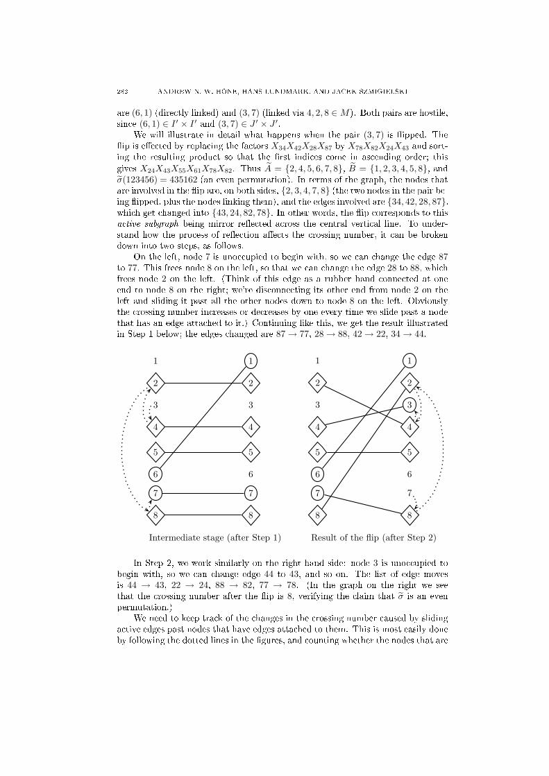
282 ANDREW N. W. HONE, HANS LUNDMARK, AND JACEK SZMIGIELSKIare (6, 1) (dire tly linked) and (3, 7) (linked via 4, 2, 8 ∈M). Both pairs are hostile,sin e (6, 1) ∈ I ′ × I ′ and (3, 7) ∈ J ′ × J ′.We will illustrate in detail what happens when the pair (3, 7) is ipped. Theip is ee ted by repla ing the fa tors X34X42X28X87 by X78X82X24X43 and sort-ing the resulting produ t so that the rst indi es ome in as ending order; thisgives X24X43X55X61X78X82. Thus A = 2, 4, 5, 6, 7, 8, B = 1, 2, 3, 4, 5, 8, andσ(123456) = 435162 (an even permutation). In terms of the graph, the nodes thatare involved in the ip are, on both sides, 2, 3, 4, 7, 8 (the two nodes in the pair be-ing ipped, plus the nodes linking them), and the edges involved are 34, 42, 28, 87,whi h get hanged into 43, 24, 82, 78. In other words, the ip orresponds to thisa tive subgraph being mirror ree ted a ross the entral verti al line. To under-stand how the pro ess of ree tion ae ts the rossing number, it an be brokendown into two steps, as follows.On the left, node 7 is uno upied to begin with, so we an hange the edge 87to 77. This frees node 8 on the left, so that we an hange the edge 28 to 88, whi hfrees node 2 on the left. (Think of this edge as a rubber band onne ted at oneend to node 8 on the right; we're dis onne ting its other end from node 2 on theleft and sliding it past all the other nodes down to node 8 on the left. Obviouslythe rossing number in reases or de reases by one every time we slide past a nodethat has an edge atta hed to it.) Continuing like this, we get the result illustratedin Step 1 below; the edges hanged are 87 → 77, 28 → 88, 42 → 22, 34 → 44.
1 1
2 2
3 3
4 4
5 5
6 6
7 7
8 8
Intermediate stage (after Step 1)
1 1
2 2
3 3
4 4
5 5
6 6
7 7
8 8
Result of the flip (after Step 2)In Step 2, we work similarly on the right-hand side: node 3 is uno upied tobegin with, so we an hange edge 44 to 43, and so on. The list of edge movesis 44 → 43, 22 → 24, 88 → 82, 77 → 78. (In the graph on the right we seethat the rossing number after the ip is 8, verifying the laim that σ is an evenpermutation.)We need to keep tra k of the hanges in the rossing number aused by slidinga tive edges past nodes that have edges atta hed to them. This is most easily doneby following the dotted lines in the gures, and ounting whether the nodes that are

EXPLICIT MULTIPEAKON SOLUTIONS OF NOVIKOV'S EQUATION 283marked (with ir les and diamonds) are passed an even or an odd number of times.However, sin e the a tive subgraph simply gets ree ted, the rossings among itsedges will be the same before and after the ip, so we need in fa t only ount howmany times we pass a passive marked node. (The passive nodes in the example are1, 5, 6.)If a passive node belonging toM is passed in Step 1, then it is passed the samenumber of times in Step 2 as well, sin e the nodes inM are marked both on the leftand on the right. Therefore they do not ae t the parity of the rossing numbereither, and we an ignore the nodes marked with diamonds, and only look at thepassive ir led nodes (all the nodes in A′ and B′ ex ept for the two a tive nodesthat are being ipped).Passive nodes belonging to A′ are ounted only in Step 1 and passive nodesin B′ only in Step 2; they get ounted an odd number of times if they lie between thetwo ipped nodes (like node 6 in the example, ounted on e), and an even numberof times otherwise (like node 1, never ounted). Consequently, what determineswhether the parity of the rossing number hanges is the number of nodes betweenthe ipped ones that belong to A′ ∪ B′ = I ′ ∪ J ′. And for a friendly pair, thisnumber is even, while for a hostile pair, it is odd.This shows that the rossing number keeps its parity (so that (−1)σ = (−1)eσ)when a friendly pair is ipped, and the opposite when a hostile pair is ipped. Theproof is nally omplete. Appendix B. Veri ation of the Lax pair for peakonsThe purpose of this appendix is to arefully verify that the Lax pair formulation(4.1)(4.2) of the Novikov equation really is valid for the lass of distributionalsolutions that we are onsidering. This is not at all obvious, as should be learfrom the omputations below.B.1. Preliminaries. We will need to be more pre ise regarding the notationhere than in the main text. A word of warning right away: our notation for deriva-tives here will dier from that used in the rest of the paper (where subs ripts shouldbe interpreted as distributional derivatives).To begin with, given n smooth fun tions x = xk(t) su h that x1(t) < · · · <xn(t), let x0(t) = −∞ and xn+1(t) = +∞, and let Ωk (for k = 0, . . . , n) denote theregion xk(t) < x < xk+1(t) in the (x, t) plane.Our omputations will deal with a lass that we denote PC∞, onsisting ofpie ewise smooth fun tions f(x, t) su h that the restri tion of f to ea h regionΩk is (the restri tion to Ωk of) a smooth fun tion f (k)(x, t) dened on an openneighbourhood of Ωk (so that f (k) and its partial derivatives make sense on the urves x = xk(t)). For ea h xed t, the fun tion f(·, t) denes a regular distributionTf in the lass D′(R), depending parametri ally on t (and written Tf (t) whereneeded). After having made lear exa tly what is meant, we will mostly be lessstri t, and write f instead of Tf for simpli ity.The values of f on the urves x = xk(t) need not be dened; the fun tion denesthe same distribution Tf no matter what values are assigned to f(xk(t), t). But ourassumptions imply that the left and right limits of f exist, and (suppressing the timedependen e) they will be denoted by f(x−k ) := f (k−1)(xk) and f(x+
k ) := f (k)(xk),

284 ANDREW N. W. HONE, HANS LUNDMARK, AND JACEK SZMIGIELSKIrespe tively. The jump and the average of f at xk will be denoted by(B.1) [f(xk)
]:= f(x+
k ) − f(x−k ) and ⟨f(xk)
⟩:=
f(x+k ) + f(x−k )
2,respe tively. They satisfy the produ t rules(B.2) [
fg]
=⟨f⟩[g]+[f]⟨g⟩,
⟨fg⟩
=⟨f⟩⟨g⟩
+ 14
[f][g].We will use subs ripts to denote partial derivatives in the lassi al sense, sothat (for example) fx denotes the pie ewise smooth fun tion whose restri tion to
Ωk is given by ∂f (k)/∂x (and whose values at x = xk(t) are in general undened).On the other hand, Dx will denote the distributional derivative, whi h in additionpi ks up Dira delta ontributions from jump dis ontinuities of f at the urvesx = xk(t). That is, DxTf = Tfx
+∑n
k=1
[f(xk)
]δxk
, or, in less stri t notation,(B.3) Dxf = fx +
n∑
k=1
[f(xk)
]δxk
.The time derivative Dt is dened as a limit in D′(R),(B.4) DtTf(t) = limh→0
Tf (t+ h) − Tf (t)
h,and it ommutes with Dx by the ontinuity of Dx on D′(R). For our lass PC∞ ofpie ewise smooth fun tions, we have DtTf = Tft
−∑nk=1 xk
[f(xk)
]δxk
, or simply(B.5) Dtf = ft −n∑
k=1
xk
[f(xk)
]δxk
,where xk = dxk/dt. We also note that ddtf(x±k (t), t) = fx(x±k (t), t) xk(t)+ft(x
±k (t), t),whi h gives
ddt
[f(xk)
]=[fx(xk)
]xk +
[ft(xk)
],
ddt
⟨f(xk)
⟩=⟨fx(xk)
⟩xk +
⟨ft(xk)
⟩.
(B.6)B.2. The problem of multipli ation. If the fun tion f is ontinuous atx = xk, then the Dira delta at xk an be multiplied by the orresponding distri-bution Tf a ording to the well-known formula(B.7) Tf δx = f(xk) δxk
.But below we will have to onsider this produ t for fun tions in the lass PC∞des ribed above, where the value f(xk) is not dened. It will turn out that inthe present ontext, the right thing to do is to use the average value of f at thejump, and thus dene Tf δx :=⟨f(xk)
⟩δxk
. However, sin e we want this to bea onsequen e of the analysis, rather than an a priori assumption, we will, tobegin with, just assign a hypotheti al value f(xk) and use that value in (B.7).This assignment is justied in the present ontext, as we will see below. However,we are not laiming that this addresses any of the deeper issues; for example, thisassignment does not respe t the produ t stru ture of pie ewise ontinuous fun tions.See [49, Ch. 5 for more information about the stru tural problems asso iated withany attempt to dene a produ t of distributions in D′(R).

EXPLICIT MULTIPEAKON SOLUTIONS OF NOVIKOV'S EQUATION 285B.3. Distributional Lax pair. Peakon solutions(B.8) u(x, t) =
n∑
k=1
mk(t) e−|x−xk(t)|belong to the pie ewise smooth lass PC∞. They are ontinuous and satisfyDxu = ux =
n∑
k=1
mk sgn(xk − x) e−|x−xk|,
D2xu = Dx(ux) = uxx +
n∑
k=1
[ux(xk)
]δxk
= u+
n∑
k=1
(−2mk) δxk,whi h implies(B.9) m := u−D2
xu = 2n∑
k=1
mk δxk.The Lax pair (4.1)(4.2) will involve the fun tions u and Dxu, as well as the purelysingular distribution m. We will take ψ1, ψ2, ψ3 to be fun tions in PC∞, andseparate the regular (fun tion) part from the singular (Dira delta) part. Theformulation obtained in this way reads(B.10) DxΨ = LΨ, DtΨ = AΨ,where Ψ = (ψ1, ψ2, ψ3)
t,(B.11) L = L+ 2z
(n∑
k=1
mk δxk
)N, L =
0 0 10 0 01 0 0
, N =
0 1 00 0 10 0 0
,and(B.12) A = A− 2z
(n∑
k=1
mk u(xk)2δxk
)N, A =
−uux ux/z u2
x
u/z −1/z2 −ux/z−u2 u/z uux
.Note that (B.10) involves multiplying NΨ = (ψ2, ψ3, 0) by δxk, and some value
ψ2(xk) must be assigned in order for this to be well-dened (we will soon see thatψ3 must be ontinuous and therefore it is only ψ2 that presents any problems).Theorem B.1. Provided that the produ t mψ2 is dened using the averagevalue ψ2(xk) :=
⟨ψ2(xk)
⟩ at the jumps,(B.13) mψ2 := 2
n∑
k=1
mk
⟨ψ2(xk)
⟩δxk
,the following statement holds. With u and m given by (B.8)(B.9), and with Ψ ∈PC∞, the Lax pair (B.10)(B.12) satises the ompatibility ondition DtDxΨ =DxDtΨ if and only if the peakon ODEs (3.4) are satised: xk = u(xk)2 and mk =−mk u(xk)
⟨ux(xk)
⟩.Proof. For simpli ity, we will write just ∑ instead of ∑nk=1. Identifying oe ients of δxk
in the two Lax equations (B.10) immediately gives [Ψ(xk)]
=
2zmkNΨ(xk) and−xk
[Ψ(xk)
]= −2zmku(xk)2NΨ(xk), respe tively. Thus, [ψ3(xk)] =

286 ANDREW N. W. HONE, HANS LUNDMARK, AND JACEK SZMIGIELSKI0 (in other words, ψ3 is ontinuous) and xk = u(xk)2. Next we ompute the deriva-tives of (B.10):
Dt(DxΨ) = Dt(LΨ + 2z(∑
mk δxk
)NΨ)
= L(AΨ) + 2zN∑
ddt
(mkΨ(xk)
)δxk
− 2zN∑
mkΨ(xk)xkδ′xk,
Dx(DtΨ) = Dx(AΨ − 2z(∑
mk u(xk)2δxk
)NΨ)
= (AΨ)x +∑[
AΨ(xk)]δxk
− 2zN∑
mkΨ(xk)u(xk)2δ′xk.The regular part of (B.10) gives Ψx = LΨ, so that (AΨ)x = AxΨ + ALΨ, andit is easily veried that LA = Ax + AL holds identi ally (sin e uxx = u). Thisimplies that the regular parts of the two expressions above are equal, and theterms involving δ′xk
are also equal sin e xk = u(xk)2. Therefore the ompatibility ondition Dt(DxΨ) = Dx(DtΨ) redu es to an equality between the oe ientsof δxk,(B.14) −2zmku(xk)2LNΨ(xk) + 2zN d
dt
(mkΨ(xk)
)=[AΨ(xk)
].Using the produ t rule (B.2), the expression for [Ψ(xk)
] above, and [ux(xk)]
=−2mk, we nd that the right-hand side of (B.14) equals(B.15) ⟨
A(xk)⟩2z mkNΨ(xk) +
[A(xk)
]⟨Ψ(xk)
⟩=
2zmk
(0 −u
⟨ux
⟩ ⟨ux
⟩/z
0 u/z −1/z2
0 −u2 u/z
)
xk
Ψ(xk) + 2mk
(u −1/z −2
⟨ux
⟩
0 0 1/z0 0 −u
)
xk
⟨Ψ(xk)
⟩.The (3,2) entry −u2 in the matrix in the rst term will an el against the wholerst term on the left-hand side of (B.14), sin e the only nonzero entry of LN is
(LN)32 = 1. Thus (B.14) is equivalent to(B.16) mk NΨ(xk) +mk NddtΨ(xk) =
mk
(0 −u
⟨ux
⟩ ⟨ux
⟩/z
0 u/z −1/z2
0 0 u/z
)
xk
Ψ(xk) +mk
(u/z −1/z2 −2
⟨ux
⟩/z
0 0 1/z2
0 0 −u/z
)
xk
⟨Ψ(xk)
⟩.To make it lear how the assumption (B.13) enters the proof, we want to avoidassigning a value to ψ2(xk) for as long as possible. Therefore we an't ompute
ddtΨ(xk) quite yet. But ⟨Ψ(xk)
⟩ is well-dened, and its time derivative an be omputed using Ψx = LΨ and Ψt = AΨ in (B.6):N d
dt
⟨Ψ(xk)
⟩= N
⟨LΨ(xk)
⟩xk +N
⟨AΨ(xk)
⟩
= N(Lu(xk)2 +
⟨A(xk)
⟩)⟨Ψ(xk)
⟩+N 1
4
[A(xk)
][Ψ(xk)
]
=
(u/z −1/z2 −
⟨ux
⟩/z
0 u/z u⟨
ux
⟩0 0 0
)
xk
⟨Ψ(xk)
⟩+ 1
4 N[A(xk)
]N
︸ ︷︷ ︸=0
2z mkΨ(xk).

EXPLICIT MULTIPEAKON SOLUTIONS OF NOVIKOV'S EQUATION 287A bit of manipulation using this result, as well as ⟨ψ3
⟩(xk) = ψ3(xk), shows thatthe ompatibility ondition (B.16) an be written as(B.17) mkN
ddt
(Ψ(xk) −
⟨Ψ(xk)
⟩)+(mk +mku(xk)
⟨ux(xk)
⟩)NΨ(x)
= mk
(0 0 00 u/z 00 0 0
)
xk
(Ψ(xk) −
⟨Ψ(xk)
⟩)The third row is zero, and the rst two rows say that(mk +mku(xk)
⟨ux(xk)
⟩)ψ2(xk) = −mk
ddt
(ψ2(xk) −
⟨ψ2(xk)
⟩),
(mk +mku(xk)
⟨ux(xk)
⟩)ψ3(xk) = 1
zmk u(xk)(ψ2(xk) −
⟨ψ2(xk)
⟩).At this point we hoose to assign ψ2(xk) :=
⟨ψ2
⟩(xk), and then it is lear that(B.17) is satised if and only if
mk = −mku(xk)⟨ux(xk)
⟩.
Referen es[1 Ri hard Beals, David H. Sattinger, and Ja ek Szmigielski. Multi-peakons and a theorem ofStieltjes. Inverse Problems, 15(1):L1L4, 1999.[2 Ri hard Beals, David H. Sattinger, and Ja ek Szmigielski. Multipeakons and the lassi almoment problem. Advan es in Mathemati s, 154:229257, 2000.[3 Mar o Bertola, Mi hael Gekhtman, and Ja ek Szmigielski. Cau hy biorthogonal polynomials.arXiv:0904.2602 [math-ph, 2009.[4 Mar o Bertola, Mi hael Gekhtman, and Ja ek Szmigielski. The Cau hy twomatrix model.Comm. Math. Phys., 287(3):9831014, 2009.[5 Mar o Bertola, Mi hael Gekhtman, and Ja ek Szmigielski. Cubi string boundary value prob-lems and Cau hy biorthogonal polynomials. arXiv:0904.2188 [nlin.SI, 2009.[6 Harish S. Bhat and Razvan C. Fete au. A Hamiltonian regularization of the Burgers equation.Journal of Nonlinear S ien e, 16(6):615638, De ember 2006.[7 Alberto Bressan and Adrian Constantin. Global onservative solutions of the CamassaHolmequation. Ar h. Ration. Me h. Anal., 183(2):215239, 2007.[8 Alberto Bressan and Adrian Constantin. Global dissipative solutions of the CamassaHolmequation. Anal. Appl. (Singap.), 5(1):127, 2007.[9 Roberto Camassa and Darryl D. Holm. An integrable shallow water equation with peakedsolitons. Phys. Rev. Lett., 71(11):16611664, 1993.[10 Giuseppe M. Co lite and Kenneth H. Karlsen. On the well-posedness of the DegasperisPro esi equation. J. Fun t. Anal., 233(1):6091, 2006.[11 Giuseppe M. Co lite and Kenneth H. Karlsen. On the uniqueness of dis ontinuous solutionsto the DegasperisPro esi equation. J. Dierential Equations, 234(1):142160, 2007.[12 Adrian Constantin. The traje tories of parti les in Stokes waves. Invent. Math., 166(3):523535, 2006.[13 Adrian Constantin and Joa him Es her. Wave breaking for nonlinear nonlo al shallow waterequations. A ta Math., 181(2):229243, 1998.[14 Adrian Constantin and Joa him Es her. Parti le traje tories in solitary water waves. Bull.Amer. Math. So . (N.S.), 44(3):423431 (ele troni ), 2007.[15 Adrian Constantin and David Lannes. The hydrodynami al relevan e of the CamassaHolmand DegasperisPro esi equations. Ar h. Ration. Me h. Anal., 192(1):165186, 2009.[16 Adrian Constantin and Henry P. M Kean. A shallow water equation on the ir le. Comm.Pure Appl. Math., 52(8):949982, 1999.[17 Adrian Constantin and Walter A. Strauss. Stability of peakons. Comm. Pure Appl. Math.,53(5):603610, 2000.[18 Antonio Degasperis, Darryl D. Holm, and Andrew N. W. Hone. A new integrable equationwith peakon solutions. Theoreti al and Mathemati al Physi s, 133:14631474, 2002.

288 ANDREW N. W. HONE, HANS LUNDMARK, AND JACEK SZMIGIELSKI[19 Antonio Degasperis and Mi hela Pro esi. Asymptoti integrability. In A. Degasperis andG. Gaeta, editors, Symmetry and perturbation theory (Rome, 1998), pages 2337. WorldS ienti Publishing, River Edge, NJ, 1999.[20 Harry Dym and Henry P. M Kean. Gaussian pro esses, fun tion theory, and the inversespe tral problem. A ademi Press [Har ourt Bra e Jovanovi h Publishers, New York, 1976.Probability and Mathemati al Statisti s, Vol. 31.[21 Khaled El Dika and Lu Molinet. Exponential de ay of H1-lo alized solutions and stability ofthe train of N solitary waves for the CamassaHolm equation. Philos. Trans. R. So . Lond.Ser. A Math. Phys. Eng. S i., 365(1858):23132331, 2007.[22 Sergey Fomin and Andrei Zelevinsky. Total positivity: Tests and parametrizations. Math.Intelligen er, 22(1):2333, 2000.[23 Felix R. Gantma her. The theory of matri es. Vol. 1. AMS Chelsea Publishing, Providen e,RI, 1998. Translated from the Russian by K. A. Hirs h, Reprint of the 1959 translation.[24 Felix R. Gantma her and Mark G. Krein. Os illation matri es and kernels and small vibra-tions of me hani al systems. AMS Chelsea Publishing, Providen e, RI, revised edition, 2002.Translation based on the 1941 Russian original, edited and with a prefa e by Alex Eremenko.[25 Ira Gessel and Gérard Viennot. Binomial determinants, paths, and hook length formulae.Adv. in Math., 58(3):300321, 1985.[26 Helge Holden and Xavier Raynaud. Global onservative multipeakon solutions of theCamassaHolm equation. J. Hyperboli Dier. Equ., 4(1):3964, 2007.[27 Helge Holden and Xavier Raynaud. Global dissipative multipeakon solutions of the CamassaHolm equation. Comm. Partial Dierential Equations, 33(10-12):20402063, 2008.[28 Darryl D. Holm and Andrew N. W. Hone. A lass of equations with peakon and pulsonsolutions. Journal of Nonlinear Mathemati al Physi s, 12(2):4662, 2005.[29 Darryl D. Holm and Martin F. Staley. Nonlinear balan e and ex hange of stability in dynami sof solitons, peakons, ramps/ lis and leftons in a 1 + 1 nonlinear evolutionary PDE. Phys.Lett. A, 308(56):437444, 2003.[30 Darryl D. Holm and Martin F. Staley. Wave stru ture and nonlinear balan es in a family ofevolutionary PDEs. SIAM J. Appl. Dyn. Syst., 2(3):323380 (ele troni ), 2003.[31 Andrew N. W. Hone and Jing Ping Wang. Prolongation algebras and Hamiltonian operatorsfor peakon equations. Inverse Problems, 19(1):129145, 2003.[32 Andrew N. W. Hone and Jing Ping Wang. Integrable peakon equations with ubi nonlinear-ity. Journal of Physi s A: Mathemati al and Theoreti al, 41(37):372002, 2008.[33 Rossen Ivanov. On the integrability of a lass of nonlinear dispersive wave equations. J.Nonlinear Math. Phys., 12(4):462468, 2005.[34 Robin S. Johnson. CamassaHolm, Kortewegde Vries and related models for water waves.J. Fluid Me h., 455:6382, 2002.[35 Samuel Karlin. Total positivity. Vol. I. Stanford University Press, Stanford, Calif, 1968.[36 Samuel Karlin and James M Gregor. Coin iden e probabilities. Pa i J. Math., 9:11411164, 1959.[37 Jennifer Kohlenberg, Hans Lundmark, and Ja ek Szmigielski. The inverse spe tral problemfor the dis rete ubi string. Inverse Problems, 23:99121, 2007.[38 Christian Krattenthaler. Advan ed determinant al ulus. Sém. Lothar. Combin., 42:Art.B42q, 67 pp. (ele troni ), 1999. The Andrews Fests hrift (Maratea, 1998).[39 Jonatan Lenells. Stability of periodi peakons. Int. Math. Res. Not., 2004(10):485499, 2004.[40 Zhiwu Lin and Yue Liu. Stability of peakons for the DegasperisPro esi equation. Comm.Pure Appl. Math., 62(1):125146, 2009.[41 Bernt Lindström. On the ve tor representations of indu ed matroids. Bull. London Math.So ., 5:8590, 1973.[42 Hans Lundmark. Formation and dynami s of sho k waves in the DegasperisPro esi equation.J. Nonlinear S i., 17(3):169198, 2007.[43 Hans Lundmark and Ja ek Szmigielski. Multi-peakon solutions of the DegasperisPro esiequation. Inverse Problems, 19:12411245, De ember 2003.[44 Hans Lundmark and Ja ek Szmigielski. DegasperisPro esi peakons and the dis rete ubi string. IMRP Int. Math. Res. Pap., 2005(2):53116, 2005.[45 Ian G. Ma donald. Symmetri fun tions and Hall polynomials. Oxford University Press, NewYork, se ond edition, 1995.

EXPLICIT MULTIPEAKON SOLUTIONS OF NOVIKOV'S EQUATION 289[46 Alexander V. Mikhailov and Vladimir S. Novikov. Perturbative symmetry approa h. J. Phys.A, 35(22):47754790, 2002.[47 Jürgen Moser. Three integrable systems onne ted with isospe tral deformations. Advan esin Mathemati s, 16:197220, 1975.[48 Vladimir Novikov. Generalisations of the CamassaHolm equation. arXiv:0905.2219 [nlin.SI,2009.[49 Laurent S hwartz. Théorie des distributions. Tome I. A tualités S i. Ind., no. 1091 = Publ.Inst. Math. Univ. Strasbourg 9. Hermann & Cie., Paris, 1950.[50 J. F. Toland. Stokes waves. Topol. Methods Nonlinear Anal., 7(1):148, 1996.Institute of Mathemati s, Statisti s & A tuarial S ien e, University of Kent,Canterbury CT2 7NF, United KingdomE-mail address: anwhkent.a .ukDepartment of Mathemati s, Linköping University, SE-581 83 Linköping, SwedenE-mail address: halunmai.liu.seDepartment of Mathemati s and Statisti s, University of Saskat hewan, 106Wiggins Road, Saskatoon, Saskat hewan, S7N 5E6, CanadaE-mail address: szmigielmath.usask. a


