Dynamics of the impact of ENSO flavors on precipitation 1 over La Plata Basin * 2 Laura Zamboni 1,2 , Annalisa Cherchi 1,3 , Marcelo Barreiro 4 , and Fred Kurcharski 5 3 1 Centro Euro-Mediterraneo per i Cambiamenti Climatici, Italy 4 2 Mathematics and Computer Science Division, Argonne National Laboratory, Argonne, 5 IL, USA 6 3 Istituto Nazionale di Geofisica e Vulcanologia, Italy 7 4 Facultad de Ciencias, Universidad de la Republica, Uruguay 8 5 Abdus Salam International Centre for Theoretical Physics, Earth System Physics 9 Section, Italy 10 Manuscript submitted to 11 Climate Dynamics 12 February 17, 2012 13 Corresponding author: 14 Laura Zamboni 15 Mathematics and Computer Science Division 16 Argonne National Laboratory 17 Argonne, IL (USA) 18 E-mail: [email protected]19 ∗ The submitted manuscript has been created by UChicago Argonne, LLC, Operator of Argonne National Laboratory (Argonne). Argonne, a U.S. Department of Energy Office of Science laboratory, is operated under Contract No. DE-AC02-06CH11357. The U.S. Government retains for itself, and others acting on its behalf, a paid-up nonexclusive, irrevocable worldwide license in said article to reproduce, prepare derivative works, distribute copies to the public, and perform publicly and display publicly, by or on behalf of the Government.
Transcript
Dynamics of the impact of ENSO flavors on precipitation1
over La Plata Basin∗2
Laura Zamboni1,2, Annalisa Cherchi1,3, Marcelo Barreiro4, and Fred Kurcharski53
1Centro Euro-Mediterraneo per i Cambiamenti Climatici, Italy4
2Mathematics and Computer Science Division, Argonne National Laboratory, Argonne,5
IL, USA6
3Istituto Nazionale di Geofisica e Vulcanologia, Italy7
4Facultad de Ciencias, Universidad de la Republica, Uruguay8
5Abdus Salam International Centre for Theoretical Physics, Earth System Physics9
∗The submitted manuscript has been created by UChicago Argonne, LLC, Operator of Argonne NationalLaboratory (Argonne). Argonne, a U.S. Department of EnergyOffice of Science laboratory, is operatedunder Contract No. DE-AC02-06CH11357. The U.S. Governmentretains for itself, and others actingon its behalf, a paid-up nonexclusive, irrevocable worldwide license in said article to reproduce, preparederivative works, distribute copies to the public, and perform publicly and display publicly, by or on behalfof the Government.
Abstract20
In this study we use observational datasets and two atmospheric general circula-21
tion models to demonstrate that the mechanism linking the canonical El Nino South-22
ern Oscillation (ENSO) to precipitation anomalies in La Plata Basin (LPB) during23
the austral Spring is found even when Sea Surface Temperature anomalies (SSTa) are24
largest over the central Pacific (Dateline El Nino). Corresponding to both flavors, in-25
creased (decreased) precipitation is observed during El Nino (La Nina) in LPB, while26
opposite anomalies occur to the northeast of South America (SA). In contrast, positive27
loads shift to the north when SSTa are uniform from the eastern to the central Pacific28
in what forms the additional flavor (Spread) we document here.29
Besides the dynamical features already reported in the literature for the impact of30
ENSO in LPB, we found evidence of an additional wave train emanated fromthe31
tropical Pacific meridionally toward the southern hemisphere in our modeling exper-32
iments. This wave can be a standalone pattern but also interfere and amplify the33
Pacific-South American Mode over the eastern Pacific and SA. Additionally,we pro-34
vide evidence of a Gill type of response to the east of the heating region and whose35
effects are appreciated on the local circulation over SA and thus precipitation over36
LPB.37
38
1
1 Introduction39
A number of studies have recently suggested the existence of an El Nino-like phenomenon dif-40
ferent from that previously described for the ”canonical” ENSO; among its main characteristics is41
the presence of largest Sea Surface Temperature anomalies (SSTa) over the central Pacific rather42
than closer to the South American coast. The new El Nino has been referred to as Dateline (Larkin43
and Harrison 2005a), Central Pacific (Kao and Yu 2009), Warm Pool(Kug et al. 2009), Modoki44
(Ashok et al. 2007), and Summer type (Xu and Chan 2001) El Nino. Trenberth and Stepaniak45
(2001) named the new and canonical types collectively as different ”flavors” of El Nino.46
A natural question is whether different impacts can be expected when different flavors occur.47
Sensitivities have already been reported globally (Larkin and Harrison 2005a, Ashok et al. 2007)48
as well as regionally for the USA (Larkin and Harrison 2005b, Mo 2010), Australia (Wang and49
Hendon 2007), the countries in the Pacific rim (Weng et al. 2007), and China (Feng and Li 2011).50
In the present paper, we explore the impact of different flavors of theEl Nino Southern Oscilla-51
tion (ENSO) on precipitation over La Plata Basin (LPB). The region, comprising southern Brazil,52
Uruguay, northeastern Argentina, southern Paraguay, and southern Bolivia, is particularly affected53
by the variability associated with ENSO (e.g., Aceituno 1988, Rao and Hada 1990, Grimm et54
al. 1998, Montecinos et al. 2000), since it strongly relies on agriculture and hydroelectricity55
production. The positive phase of ENSO (El Nino) tends to generate increased seasonal precip-56
itation over LPB and drier conditions over northeast South America (SA) both associated with57
anomalous intensity and direction of the South American Low-Level Jet (SALLJ) (Ferreira et al.58
2003, Liebmann et al. 2004, Silva et al. 2009). The sign of anomalies reverses during La Nina59
(Grimm et al. 2000). Hill et al. (2009) compared the 1997/98 (Eastern) and 2002/03 (Dateline)60
events searching for impacts over SA during the summer season. In their results the 1997/98 event61
presented more intense precipitation in LPB, more intense subsidence over northern SA, a more62
intense SALLJ, and a displaced Walker circulation over the ocean (Hill et al. 2011); these authors63
further proposed the presence of a more intense Pacific South American (PSA) pattern. We focus64
on the austral Spring because in this season the teleconnection between ENSO and LPB is best65
established (Cazes-Boezio et al. 2003, Zamboni et al. 2011).66
In developing the present analysis we found the need to develop an alternative criteria for iden-67
tifying the different flavors of ENSO. This is described, along with our motivations, in Section 3.68
In the following we outline as a background the methods employed in the literature.69
Defining ENSO events is per se a challenge because every event presents somewhat different char-70
2
acteristics regarding onset, duration, intensity. and evolution. Even the peak of the event, which71
can largerly be considered as locked to the seasonal cycle, has in the past occurred in seasons72
other than the boreal winter (see e.g., Neelin et al. 2000, Xiao and Mechoso 2009). Indeed no73
accepted definition of El Nino exists (Hanley et al. 2003), but noneless, different authors agree74
on identifying a set of years as ENSO events (see Fu et al. 1986 and Larkin and Harrison 2005a75
for comparisons among studies). Among these, Wang (1995) noticed that, contrary to what pre-76
viously reported (Rasmusson and Carpenter 1982), SSTa of a group of El Ni no first developed77
in the central Pacific and appeared over the eastern Pacific only afterward (see Fig.3 in Wang78
1995). Larkin and Harrison (2005a) compared 11 ”conventionally identified” events occurred79
since 1950 with a number of ”additional” events (”Dateline” El Nino), resulting from the offi-80
cial definition adopted by the USA National Oceanic and Atmospheric Administration (NOAA)81
in 2003 (http://www.cpc.ncep.noaa.gov/products/analysismonitoring/ensostuff/ensoyears.shtml).82
Ashok et al. (2007) named the second Emipirical Orthogonal Function (EOF) analysis of Pacific83
SSTs obtained from 1979-2004 ”Modoki El Nino”. Unlike other studies, these authors included an84
area over the far western Pacific (125-145 E;10S-20N) to define an index for the Modoki events,85
although the anomalies in this area are not pronunced (see their Fig. 2b). Asimilar but more86
extended analysis by Kao and Yu (2009), who also identified an ”Eastern” and ”Central” El Nino,87
shows minor anomalies over the same area, which we conclude do not reflect a significant fea-88
ture of the new flavor. Further, the index Ashok et al. (2007) introduced cannot be employed to89
cathegorize all ENSO events; for example, it would miss the El Nino event of 1997 (the El Nino90
Modoki index was -0.53 during the austral Spring of that year). Other recent definitions are based91
on large anomalies in the Nino4 region from September through February (”Warm Pool” El Nino92
of Kug et al. 2009), the onset of the events (”Spring” and ”Summer” types of Xu and Chan 2001),93
EOF and cluster analysis of Pacific SSTs (”Eastern” and ”Central” SSTaof Kao and Yu 2009). Fu94
et al. (1986) emphasized the importance of the zonal SSTa gradient in determining atmospheric95
circulation changes.96
One relevant aspect in the context of the ENSO flavors is their associationwith the decadal97
variability. A simple examination of the events we considered do indeed suggest a higher (lower)98
occurrence of Dateline (Eastern) events since the 1970s (see Table 2). Changes in the interannual99
variability (Trenberth and Stepaniak 2001), duration, onset, intensity (Kao and Yu 2009), and per-100
sistence (Yu and Kao 2007) of SSTa in different areas of the tropical Pacific have been reported, as101
well as associations with interdecadal changes in the northern tropical Pacific (Zhang et al. 1997),102
the Pacific Decadal Oscillation (Hanley et al. 2003), and its relationship with precipitation in SA103
3
(Kayano and Andreoli 2007). While research continues to add to our understanding of this aspect,104
we seek to elucidate the possible different impacts of ENSO flavors over LPB so as to anticipate105
considerations regarding decadal variation over the region and predictability.106
In sorting past events, we noticed the existence of a pattern that, to the bestof our knowledge, has107
not previously reported. This consists of approximately uniform SSTa from the South American108
coast to the central Pacific, and to which unexpected precipitation anomaliesin SA correspond109
(see Fig. 3).110
We start by discussing our method for sorting the different flavors, whose corresponding pre-111
cipitation and circulation characteristics are contrasted. Next, we discuss the dynamics of the112
different flavors using idealized and AMIP-type of experiments with the International Centre for113
Theoretical Physics Atmospheric General Circulation Model (ICTP AGCM) (previously named114
SPEEDY) (Molteni 2003) and ECHAM4 (Roeckner et al. 1996). The paper is organized as fol-115
lows. Section 2 describes the datasets we use. In Section 3 we discuss ourdefinition of the flavors.116
Section 4 compares observations and reanalysis data. Section 5 describes the models’ response to117
idealized experiment in which sintetic SSTa mimic the flavors. These results are then compared118
in Section 6 with those obtained with AMIP types of experiments. We present observational evi-119
dences of a tropical influence (Gill type of response) on precipitation in LPB in Section 7, and we120
conclude in Section 8 with a summary of our findings.121
2 Datasets, numerical models, and experiments122
In the present study we focus on the austral Spring, chosen as the average of October and Novem-123
ber to represent the coeherent signal throughout the season (Montecinos et al. 2000). The period124
of interest is 1948-2002. Our analysis compares modeling results with available reanalysis and125
observational datasets.126
The Atmospheric General Circulation Models (AGCMs) we employed are ECHAM4 (Roeck-127
ner et al., 1996) and the International Centre for Theoretical Physics (ICTP) AGCM (Molteni128
, 2003). The ICTP AGCM is an intermediate-complexity model and includes physically based129
parameterizations of large-scale condensation, shallow and deep convection, short-wave and long-130
wave radiation, surface fluxes of momentum, heat and moisture, and vertical diffusion (see also131
Kucharski et al, 2006). The ICTP AGCM has been employed in research on the South American132
Monsoon (Barreiro and Tippmann 2008) and investigations on the link between the circulation in133
the Southern Hemisphere and in SA (Zamboni et al. 2011). The configurations we used have a134
4
spectral truncation at total wavenumber T106 and 19 sigma vertical levels for ECHAM4, while 8135
vertical sigma levels and a horizontal resolution of T30 characterize the ICTP AGCM. We mainly136
discuss results obtained with ECHAM4 since they better compare with observations, although the137
ICTP AGCM provides similar dynamics (see Section 6).138
The first set of experiments we present is intended to restrict the models’ response to anomalies139
in the tropical Pacific. These anomalies, both positive and negative, are imposed on the October-140
November SST climatology and have a Gaussian shape with a maximum of2◦C (Fig. 2) centered141
in three locations so as to mimic the ENSO flavors. The experiments, consisting of30 year long142
runs for ECHAM4 and 50 year runs for the ICTP AGCM, are then subtracted from a control143
run performed with climatological SSTs to obtain anomalies. We refer to these experiments as144
”idealized experiments”. The second set consists of an Amip type ensemble,in which observed145
interannually varying SSTs have been used as boundary conditions. The results we present are146
obtained by averaging over a 9-member ensemble for ECHAM4 and a 35-member ensemble for147
the ICTP AGCM; these members differ by the atmospheric initial conditions.148
The global monthly sea surface temperature is taken from the HadISST dataset (Rayner et al.,149
2003), which is available from 1871 to the present at a resolution of1◦.150
The precipitation dataset we use was compiled by the Climate Research Unit (CRU), University151
surements. Data are available at0.5◦ x 0.5◦ horizontal resolution over land for the period 1901-154
2002 (Mitchell and Jones, 2005). We additionally employ the Climate Prediction Center Merged155
Analysis of Precipitation (CMAP) dataset (Xie and Arkin 1997) for guidance on precipitation pat-156
terns over the oceans. The data are available for the period 1979-2009, which presents a limitation157
since it covers our period of analysis only partially. This aspect is particularly severe for Eastern158
La Nina and the flavor we named ”Spread” (see Section 3), in fact all the events occurred before159
1979 for the former and only 1 out of a total of 4 dates after 1979 for the latter.160
The atmospheric fields correspond to the global National Centers for Environmental Prediction-161
National Center for Atmospheric Research (NCEP-NCAR) reanalysis; these are available at2.5◦162
x 2.5◦ horizontal resolution (Kalnay et al. 1996) from 1948 to the present.163
164
5
3 Definition of the events165
Our intention is to base the definition of Eastern and Dateline types of SSTa ontoindices having166
equal areal extension and together covering the entire eastern Pacific,from the South American167
coast to the dateline. This is not possible, however, with the standard ENSOindices. Hence, we168
introduce two new indices, Nino East (nE) and Nino West (nW), which consist of the average169
standardized SSTa over 5S-5N; 170W-130W, 5S-5N; 120W-80W, respectively1. These indices170
measure the localintensityof SSTa, which must be a minimum of±0.5 in either nE or nW to171
identify an ENSO event (Table 1). For comparison, anomalies are computedwith respect to the172
1971-2000 climatology and have the same persistence criteria as in the definition by NOAA. The173
value of the indices in Spring is used to discriminate among the flavors. In fact,at the seasonal174
scale the quick response of the atmosphere makes the simultaneous relationship between SSTa175
and precipitation in LPB the strongest (Montecinos et al. 2000). The definitions of ENSO flavors176
currently proposed in the literature are based on the onset of the events,EOF analysis, or indices177
averaged over a season; none takes the view we propose.178
The ”Eastern El Nino” pattern is characterized bylarger SSTa over the Eastern Pacific and179
smaller or no anomalies over the Central Pacific; it represents the canonical ENSO. The location180
of larger and smaller anomalies is reversed during ”Dateline El Nino” events. To describe the181
zonal gradient of SSTa we use a modified trans-Nino index (Trenberth and Stepaniak 2001) that182
consists of the standardized difference between nE and nW, which we name Trans-Nino East-West183
(TNIEW). We found a TNIEW equal to±0.3 suitable to discriminate among the flavors, while nE184
or nW equal to 0.5 sets the threshold for the intensity (Table 1). Similar considerations hold for185
La Nina but with the sign of anomalies reversed.186
In analyzing the historical record of SSTs we noticed the existence of cases in which anoma-187
lies were of approximately equal intensity from the eastern to the central tropical Pacific. Further188
inspired by corresponding unexpected precipitation anomalies over SA (see Fig. 3), we decided189
to conduce a separate analysis for this new flavor, which we named ”Spread”. To the best of our190
knowledge, no similar patterns have been considered in the literature before.191
We list in table 2 the events we consider, along with the composite of SSTa for each flavor in192
Fig. 1.193
One novel aspect of the present study is the investigation of La Nina events in the context of194
1The band 120W-130W is not represented by either nE or nW; this is chosen with the aim of reducing the sensitivity
of the stratification arising from more westward extended Eastern ENSOs and more eastward extended Dateline ENSOs.
6
ENSO flavors, which previously were studied only for the austral summer (Cazes-Boezio, per-195
sonal communication). A relevant consequence of our definition is the presence of ”Eastern” La196
Nina in our categories, which may be surprising since negative SSTa usuallyfirst develop over the197
central Pacific. We point out that our method disregards the evolution of SSTa and is thus not nec-198
essarily suitable to describe the ENSO phenomenon itself; rather, it is designed to explore impacts199
simulteneous to the occurrence of ENSO. On the other hand, we believe thatnE, nW, and TNIEW200
may prove effective in explorations of the flavors regardless of the emphasis on the simultaneous201
responses.202
203
4 Observations204
We begin our discussion by examining the effect on precipitation associatedwith the three fla-205
vors (Fig. 3). This is substantially linear in both the sign and the intensity of SSTa for Eastern206
and Dateline, in agreement with previous analyses (e.g., Grimm et al. 2000). In the remainder207
of the paper we show composites of El Nino minus La Nina for these flavors, unless otherwise208
stated. Substantially different featureslocally over SA distinguish the positive and negative phase209
of Spread; we thus show them separately.210
Eastern and Dateline feature increased loads over LPB and negative anomalies to the northeast,211
forming the see-saw pattern known as the canonical response to ENSO over SA. The largest pre-212
cipitation anomalies are found for Eastern, which may be the result of the outstanding intensity of213
SSTa during 1982 and 1997.214
Remarkably distinct patterns appear during Spread events (Fig. 3c): in both phases a wide215
region of increased precipitation is located in place of the dry conditions observed for the other216
flavors (50W-20S). These anomalies are statistically significant at the 95%level, as obtained by a217
non-parametric test, based on a bootstrap procedure using a resampling technique (Wilks 1995).218
Normal precipitation is found in LPB during Spread El Nino, while an east-west dipole character-219
izes Spread La Nina.220
Examination of reanalysis data for Eastern reveals the signature of a substantial Tropical heat-221
ing over the central Pacific and the existence of a clear wavelike pattern in the South Hemisphere222
arching from the Indian Ocean to eastern SA (Fig. 4a), which is recognized as the leading PSA223
mode (Kidson 1988). This and in particular its eastern extension, the vortexcentered at 20S-50W224
has been linked to an increased and southeastward oriented SALLJ (Zamboni et al. 2010, Diaz225
7
and Aceituno 2003), which in turn leads to increased precipitation over the subtropicalregions and226
opposite anomalies over the SACZ (Diaz and Aceituno 2003, Mo and Paegle 2001, Paegle and227
Mo 2002). The chain of elements we have just sketched represents the mechanism for the impact228
of ENSO when all past events are considered together (Zamboni et al. 2011).229
Upper level circulation anomalies for Dateline are similar to those of Eastern but less intense230
(Fig. 4b). In the Southern Hemisphere a wave train is evident, but anomaliesbetween 120E and231
180E are much less pronunced compared with those to the east. These appear the result of an ad-232
ditional wave that propagates meridionally from the central Pacific (Vera et al. 2004) and merges233
with the PSA at 120W-70S. A clear vortex is also evident over subtropicalSA.234
A circulation of smaller intensity is found for Spread, particularly over the central Pacific in the235
Norther Hemisphere (Figs. 4c,d). In the Southern Hemisphere, anomalies recall the PSA pattern,236
but opposite anomalies occur at very high latitudes and possibly interfere with the former. Of237
interest to our goals, the anticyclonic circulation over eastern SA is displaced over the Atlantic it238
influences SA only marginally during La Nina (Fig. 4d), while it is flanked by a large-scale cy-239
clone during El Nino (Fig. 4c). At low levels an intense cyclone is found inland over northernSA240
during El Nino, while an opposite westerly flow at 20S characterizes La Nina, consistently with241
respectively enhanced and reduced SALLJ toward the region of intense precipitation anomalies242
along the coast.243
Observed SSTa of the three flavors differ in relevant aspects beyondtheir location and hence244
limit the extent to which a direct comparison can be carried out. For example SSTa over the trop-245
ical Pacific during Eastern are 30% larger than those of the other flavors. As mentioned earlier,246
only three events represent the positive phase of this flavor, and thus results might depend on the247
specific features of these. Additionally, the belt of opposite anomalies in the subtropical Pacific,248
which is part of the ENSO dynamics, has been suggested as a key factor for the propagation of249
the PSA (Vera et al. 2004) and are for Spread barely noticeable. SSTain other basins introduce250
further dissimilarities among the flavors; examples are found in the Indian andsouthern Atlantic251
Oceans for Eastern and in the tropical Atlantic for Spread (see Fig. 1).252
To conduct a systematic investigation and focus on the response from the Pacific Ocean we per-253
formed a number of idealized experiments in which SSTa mimicing the three flavors(Fig. 1) have254
been superimposed onto the ON climatology in two AGCMs. We analyze these in thefollowing255
section. The results are then compared with those obtained with AMIP types ofsimulations in256
section 6 to investigate the response of the models to realistic SSTs, as well as the role of SSTa in257
other oceans.258
8
5 Idealized experiments259
The response of Echam to Eastern types of idealized SSTa consists of several of the features we260
have described in section 4, namely, the PSA, and anomalous SALLJ and precipitation anomalies261
in LPB. Clearly, the tropical Pacific accounts for much of the response wesee in the observations.262
Of further interest is the presence of an intense Gill quadrupole (Gill 1980), whose anomalous263
vortices are located above the SSTa (Fig. 5) and over the tropical Atlantic Ocean, the latter be-264
ing of smaller intensity. The circulation associated with positive SSTa is indicative of low level265
anomalous westerlies over the tropical Pacific and easterlies over the Atlantic, which thus appear266
to contribute in increasing precipitation over LPB via enhancement of the SALLJ (Fig.5c). Over267
the eastern Pacific Ocean around 30S, the baroclinic response over thetropics is accompanied by268
a barotropic wave propagating meridionally (Fig.5a,b). This is possibly generated by the vortic-269
ity source corresponding to the heating induced by tropical SSTa and intense precipitation there270
(Sardeshmukh and Hoskins 1985) and resembles the secondary wave discussed in section 4. To271
the east the interference of such a wave with the PSA is also evident.272
The higher sensitivity of the atmosphere to SSTa located over the central Pacific determines273
a stronger atmospheric response2 for Dateline, resulting in more intense Gill’s quadrupole and274
wave trains. Precipitation anomalies in SA are reproduced by the AGCM only for positive SSTa275
and over LPB. The difficulty in reproducing precipitation anomalies with a climatemodel is well276
known, and we thus continue our analysis on the more reliable dynamical fields. The dynamics277
of the response over SA consists of a pure PSA3 south of 45S, while to the north at low levels a278
broad anticyclonic circulation results from the combination of the vortex (Fig.5e) and of a baro-279
clinic circulation over the tropical Atlantic (Figs. 5d,e). This join effect leadsto an intense SALLJ280
and positive precipitation over LPB (Fig. 5f). The mechanism linking the canonical ENSO to281
precipitation anomalies in LPB is thus found even when positive SSTa are located over the central282
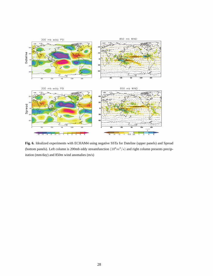
Pacific. For negative SSTa the expected cyclone over SA is lacking, as are precipitation anomalies283
over subtropical SA (Fig. 6, upper panels), while a wave train propagating from the tropics is284
present. The nonlinearity of the formation of the vortex over SA to the sign ofSSTa appears to be285
an artifact of this idealized experiment, as it is not present in either the observations or the Amip286
experiments (see Section 6). The presence of a Gill response is also found for Dateline.287
2In fact, the actual temperature is higher.3The wave train on the middle left panel of Fig. 5 could also be interpreted asthe wave propagating directly from
the location of SSTa. However, the arching pattern and the location of anomalies remarkably correspond to those of the
PSA and PNA. The same consideration holds for Spread.
9
For Spread the Gill’s quadrupole is zonally elongated (as SSTa are) and spans the entire tropical288
Pacific (Figs. 5g,h); this appears to interfere with the intensity of the PSA, whose anomalies result289
dumped. Neverthless, anomalies associated with the PSA and Pacific North American patterns are290
approximately on the same locations as those of Dateline (Fig. 5d,g), supportingthe interpretation291
that these patterns are resonant modes of the system (Robertson and Mechoso 2003) rather than292
propagating waves dependent on the precise location of their source. Corresponding to positive293
SSTa, precipitation anomalies in the model are the result of the Gill response alone, with the PSA294
pattern being confined at high latitudes, since its eastern end is lacking. Indeed, such a vortex may295
be independent of the PSA (Zamboni et al. 2011). Although at high latitudes Spread does not296
present the PSA for negative SSTa, but a zonal belt of alternate anomalies, it features a cyclonic297
circulation at 30S that, together with the circulation associated with the Gill response to the north,298
creates a precipitation dipole with centers over LPB and SACZ (Fig. 6, bottompanels). The ideal-299
ized experiment clearly misses the precipitation patterns characterizing Spread in the observations300
and produces a similar mechanism found for the other flavors.301
Summarizing, in the idealized experiments, a combination of the canonical mechanism (PSA302
and the presence of a vortex over subtropical SA) and the Gill response we have documented303
determine the impact on precipitation over LPB for Eastern and the positive phase of Dateline.304
We highlighted the leading role of the tropical Pacific in shaping the atmospheric respose and the305
capability of the model in reproducing a number of dynamical features, as well as anomalies of306
smaller intensity during La Nina for all flavors. On the other hand, we cannot draw firm conclu-307
sions on what determines the patterns of precipitation in LPB for Spread andDateline La Nina,308
the origin of the PSA pattern, and the occurrence of the vortex over SA. Clearly, further elements,309
not reproduced by the idealized experiments, determine these features. We address these aspects310
in the next section, discussing in particular the sources of the PSA and theirreproducibility with311
an AGCM.312
The Gill response we documented motivated us to explore whether it is a realfeature of the313
circulation (instead of a model’s artifact) and the extent to which it influencescirculation and314
precipitation over subtropical SA. We discuss this aspect in Section 6 usingAmip types of exper-315
iments; while in Section 7 we show its existence in the observations.316
10
6 Amip experiments and discussion317
In this section we explore the role of SSTa other than those in the tropical Pacific and draw con-318
siderations about the capability and limitations of an AGCM in reproducing the dynamics of the319
flavors, as well as their impact on precipitation in LPB. To this end, we compare results obtained320
with the idealized and Amip experimentsa and support the novel results we document with both321
ECHAM4 and the ICTP AGCM. In this regard results from the two AGCMs present only minor322
differences; and although we considered them both to corroborate ourconclusions, it would be323
reduntant to show the results for the ICTP AGCM with additional detail.324
The dynamics and response for Eastern El Nino are similar between the idealized and Amip325
experiments (Figs. 7a,b), confirming that the model’s response is largely driven by the tropical326
Pacific. The Gill response is less intense and more extended into the centralPacific during El Nino327
in the Amip experiment (Figs. 7a,b); a more marked PSA pattern is also presentand compares328
remarkably well with the observations (Fig. 4a). Similar to the observations, but not the idealized329
experiments, opposite precipitation anomalies accompanied by upper-level divergence (conver-330
gence) are found over the eastern and central (western) Pacific (Fig.7c). This difference between331
the Amip and idealized experiments suggests that even though the largest SSTa are located over332
the east during Eastern, the more extended pattern into the central Pacific,featured in the obser-333
vations but not in the idealized experiments, plays a key role in shaping the Walker circulation.334
We posit that the upper-level divergence over the central Pacific induces dry conditions and upper-335
level convergence at 120E, which in turn establishes the PSA, in agreement with the Rossby waves336
sources (RWS) we explored4. For example, during Eastern La Nina the Amip experiment does not337
present either the PSA or the upper level divergence at 120E (Fig. 7d). As in the observations, the338
AGCMs we employed do reproduce a smaller response during La Nina, but they require stronger339
SSTa to trigger the PSA, while a clear wave emanated from the central Pacificis evident in the340
Amip experiment. The asymmetry in the response for the two phases of Easternmay originate341
over the western Pacific between 150W and180W, a region in which SSTa of Eastern La Nina342
are substantially less intense than those of El Nino. The lack of a corresponding well-reproduced343
precipitation pattern over the western Pacific and Indian Ocean is a general drawback of current344
AGCMs, and it is due to the lack of atmosphere-ocean feedbacks over theregion in this type of345
experiments. The lack of positive SSTa over the subtropics in the southernPacific during La Nina346
can also play a role (Vera et al. 2004).347
4In the following we show precipitation patterns since the patterns of RWS are noisy.
11
For Dateline the upper-level divergence is less intense in the Amip experiments (Fig. 8), con-348
verge to the west is minor, and the PSA is absent, different from the markedextratropical tele-349
connection seen in the idealized experiments (Fig. 5d). The precipitation pattern over the central350
and western Pacific is similar for Eastern and Dateline in both the Amip experiment(Fig. 7c and351
Fig. 8c) and the observations (Fig. 9), but the intensity of both SSTa and precipitation anomalies352
is double for Eastern. Comparing the SST patterns, one can see that anomalies for Eastern and353
Dateline are similar over the central Pacific, while larger anomalies exist to the east for Eastern.354
We conclude that the largest response during Eastern is determined by theoutstanding intensity of355
a wide, zonally extended pattern of SSTa. In the subtropics over the Pacific, SSTa are substantial356
during Dateline, and we thus deduce that their role in determining the PSA is significantly minor357
compared with that of theintensityof SSTa over the tropics.358
Dateline also features a wave extending meridionally from the tropics for bothEl Nino (Fig. 8)359
and La Nina (not shown); a result that is also obtained with the ICTP AGCM (Fig. 10a).360
We anticipated in Section 5 the presence of the vortex over SA only in the Amip experiment for361
Dateline La Nina. As discussed, we found that the Gill response tends to be too strong and merid-362
ionally extended in the idealized experiments, while it is significantly less intense inthe Amip363
experiments, especially to the east for both ECHAM (Fig. 8) and the ICTP AGCM (Fig. 10).364
Nevertheless, its influence on the SALLJ (Fig. 8c) and thus precipitation in LPB are recognized.365
The dynamics for Spread El Nino is the same for the two experiments, but anomalies are smaller366
in the Amip, in particular, no precipitation anomalies appear over SA (not shown). The AGCMs367
produce no significant anomalies in the extratropics, a feature possibly indicative of an excessively368
strong atmospheric response to zonally extended SSTa. As already noticed, the models’ response369
to La Nina is smaller over the tropics, and the Amip experiment produces circulation anomalies in370
the extratropics and the secondary wave (Fig. 8). However, the model proposes the same dynamics371
as for the other flavors and anomalies substantially different from those seen in the observations.372
7 Role of the Gill response in precipitation in LPB373
In the previous sections we discussed the influence of a Gill type of response on precipitation over374
LPB we saw in the modeling experiments we conducted. The latter accompanies the more docu-375
mented Gill response found to the west of SSTa and consists of upper level cyclonic (anticyclonic)376
vortices to theeastof positive (negative) SSTa. At low levels it strenghtens (reduces) thetrade377
winds over the Atlantic and consequently the intensity of the SALLJ toward LPB. In this section378
12
we show evidence of this circulation in the observations.379
Exhamination of the eddy streamfunction at different vertical levels showsfor Eastern the two380
anticyclonic vortices straddling the equator over the eastern Pacific, typical of the Gill response,381
from 400 mb (Fig. 11a) and above. Over the same range of altitudes two lessintense cyclonic vor-382
tices are present at 80W-5S and 15N, which may indeed represent the circulation we are seeking.383
Above 400 mb, the signal strengthens (not shown). At lower levels the circulation is opposite; and384
although patterns are less neat, two anticyclonic circulations are present at 60W-10S and 10N. The385
eastern component of the Gill response is found to have smaller intensity in both the numerical386
experiments and in the observations, which is expected because of the competing signal sourced in387
the Atlantic Warm Pool. The Amazon also represents an important source of heating; and since its388
role cannot be represented in an Amip experiment, a model including dynamic vegetation would389
elucidate this aspect. A dumping of the southeastern vortex of the Gill response by the barotropic390
vortex over subtropical SA is also plausible for Eastern since the latter extends into tropical lati-391
tudes.392
For Dateline two zonally extended cyclones are present at 400 mb at tropical latitudes on either393
side of the equator between 80W-40W (Fig. 11c), while at low levels a vortex is present at 10N-394
80W but not to the south. Hence, for this flavor, the impact of the Gill response on circulation over395
tropical SA is minor (Figs. 11c,d).396
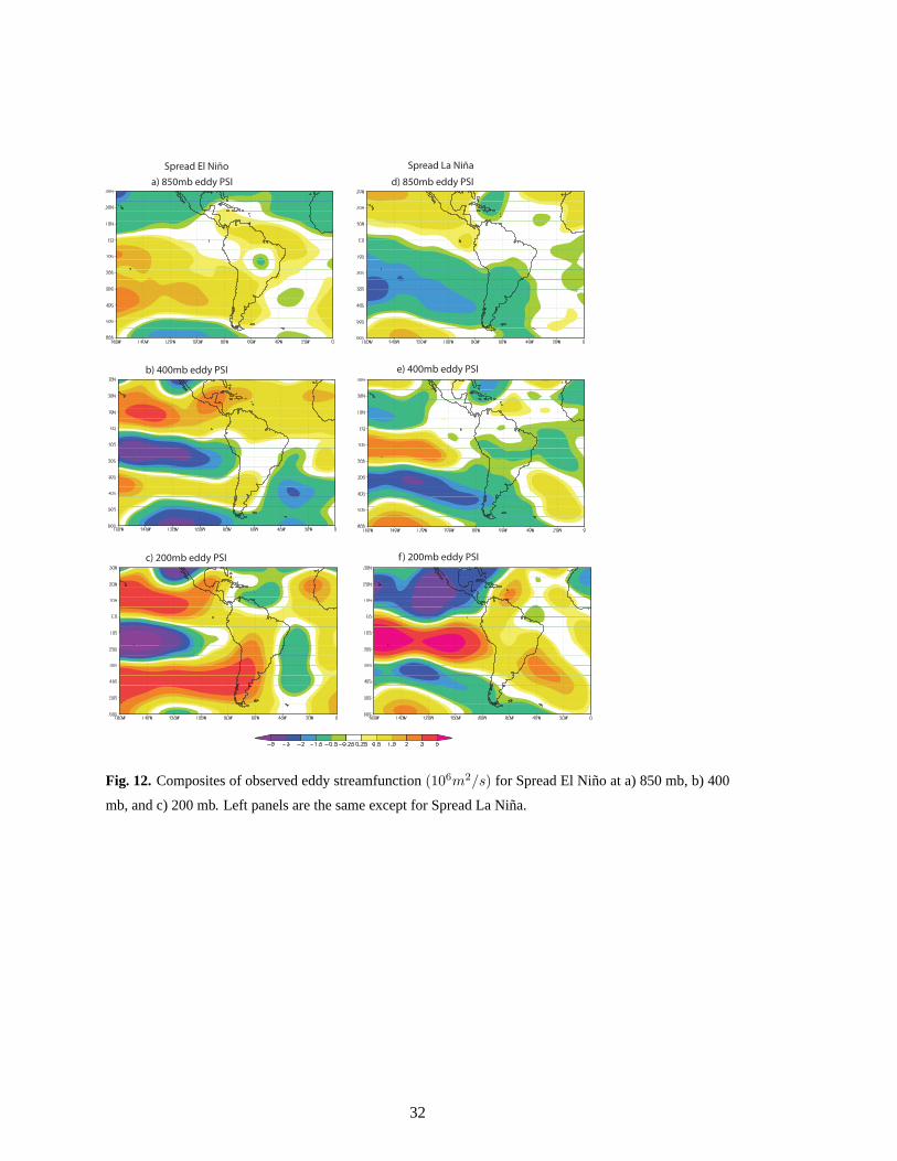
During Spread El Nino an intense low-level anticyclone at 15S-50W diverts the SALLJ toward397
northeastern Brazil, where a region of convergence is found (Fig. 12a). The same rotation is398
visible up to 500 mb (not shown). We interpret the remarkable intensity and extension of this399
vortex as the result of the Gill response and local forcings. In exploring this aspect we suggest400
investigating the role of local effects, for example, vegetation and soil moisture, which have been401
shown to impact the local circulation during ENSO (Grimm et al. 2007). At upper levels a cy-402
clone is present at 60W-10N, consistently with a Gill response, but to the south the other pole is403
destroyed (Fig. 12c). The latter is possibly overcome by the cyclonic circulation associated with404
the secondary wave at 30-40S; 60W (Figs. 12b,c). The reasons behind the presence of such a405
strong signal remain unclear at present.406
A small vortex at 10-20N; 60W during Spread La Nina is seen throughout the atmospheric col-407
umn (Fig. 12). An opposite circulation is detected at 400 mb across SA over 10S, but at upper408
levels the latter circulation is then overcome by the increased effect of the cyclone over subtropical409
SA (Figs. 12e,f).410
A number of features differentiates Spread from Eastern and Dateline and its lack of linearity411
13
between the positive and negative phases. Local effects appear to have played a relevant role in412
shaping precipitation and circulation anomalies during these past events. Land processes, which413
could not be exploited by the experiments we conducted but likely are important at the beginning414
of the rainy season in northern SA, deserve more attention in future studies. On the other hand,415
anomalies associated with the secondary wave are remarkably zonally extended over the subtrop-416
ics at upper levels during Spread. These appear to influence the circulation over SA directly rather417
than via an extratropical connection as it is for Dateline.418
8 Summary419
In this paper we have explored to what extent precipitation anomalies in La Plata Basin (LPB)420
during the Spring season are sensitive to SSTa located in different areas of the tropical Pacific.421
In these patterns of SST, referred to in the literature as ENSO flavors, thelargest anomalies are422
located over the east or around the dateline during Eastern and Dateline events, respectively.423
We introduced three indices representing the areal average of SSTa over the eastern (nE), the424
central Pacific (nW) and their difference (TNIEW) to quantify the intensityand zonal gradient425
of SSTa, respectively. These indices are more suitable for investigationsof ENSO flavors since426
they cover areas of equal estension in the region where larger SSTa occur, a goal that cannot be427
achieved with the standard El Nino indices (see Section 3).428
In investigating the events occurred during 1948-2002, we noticed the existence of SST patterns429
in which anomalies have a uniform intensity from the eastern to the central Pacific; we named this430
new flavor Spread (Fig. 1). An additional novel aspect of the present study is the analysis of La431
Nina, since investigations in the context of the flavors have so far focusedon El Nino only.432
To conduct this research, we employed observational and reanalysis data as well as numerical433
experiments performed with two AGCMs. We realized a set of idealized experiments in which434
SSTa mimicing of the flavors have been superimposed to the climatology for ON first; then we435
performed a set of Amip type of experiments aimed to determine the relative role of SSTa over the436
Pacific and other basins.437
Contrary to our expectations, we found a similar precipitation pattern for the Eastern and Date-438
line flavors. This consists of increased precipitation over LPB and decreased precipitation to the439
north over the SACZ; the pattern reverses during La Nina. These results are comparable to those440
obtained by Hill et al. (2011) for the summer season. Particularly relevantprecipitation anomalies441
during Spread consist of positive loads in place of dry conditions occurring for the other flavors at442
14
20S along the Atlantic coast of SA (Fig. 3).443
Precipitation anomalies in LPB are linked to the circulation upstream, namely, the Pacific-South444
American Mode (PSA; Mo and Paegle 2001, Casez-Boezio et al. 2003, Paegle and Mo 2002),445
whose establishment occurs via reduced precipitation and upper-level convergence over the west-446
ern Pacific, which is in turn driven by convection over the central Pacific. Keys in driving the447
anomalous Walker circulation are SSTa between 150W and 180W but also intense anomalies over448
the eastern Pacific when anomalies are present over the central Pacific.Further, the intensity of449
SSTa, rather than their location or the presence of opposite anomalies in the subtropics (Vera et al.450
2004) is the leading factor in determining the response.451
Corresponding to intense SSTa extended into the central Pacific, as for example during the event452
of 1982 and 1997, we found the AGCMs we employed were able to reproduce the PSA and the453
pattern of precipitation over the ocean partially. However, this is not the case when smaller SSTa454
occur and reveal the importance of the atmosphere-ocean interaction occurring there.455
We documented the existence of an additional wave train emanated from the region of the main456
heating. This is noticed in the observed past events and is reproduced in the modelling experiments457
we performed. Such a wave train, first documented by Vera et al.(2004), has a strong meridional458
propagation, is present during Dateline, and is prominent during Spread. During Spread, it ap-459
pears so intense that is modifies the extratropical connection by shifting it to the north at 120W,460
while during Dateline a clear interference with the PSA occurs east of 120W(Fig. 4). Further461
explorations would benefit our understanding of its interation with the PSA, the formation of the462
vortex over subtropical SA, and thus precipitation anomalies over LPB.463
Locally over SA circulation anomalies are driven by the presence of a continental-scale vortex,464
which is often, but not always, the eastern end of the PSA (Zamboni et al. 2011). This vortex is465
present for all flavors, but relevant variations in its position are not accounted for by SSTa. Rather,466
local effects may play an important role and deserve more investigation, forexample by using of467
a model with dynamic vegetation. Further, the vortex over SA and an intense SALLJ are found468
even when the PSA is not, for example during Dateline events (see Fig. 4), suggesting that the469
secondary wave can also trigger their occurrence.470
The idealized experiments suggest the existence of a Gill type of responseto the east of the heat-471
ing region, with effects impacting the circulation locally over SA and thus precipitation over LPB.472
To our knowledge, this mechanism has never been reported in the literature. We thus searched for473
this signal in the observed past events and indeed found proof of its existence (see Section 7). The474
intensity of the vortices to the east of the heating region is significantly smaller in the observations475
15
than in the model, especially at low levels, but it still appears to influence precipitation via modu-476
lation of the intensity of the SALLJ for Eastern. No significant anomalies are found at low levels477
for Dateline, whereas the circulation for Spread is particularly strong andthus possibly amplified478
by local effects. Indeed, our modeling experiments provide an overly strong response to El Nino,479
while the same response seen for the other flavors corresponds to that of Spread La Nina. We480
emphasize the need for exploring these local impacts to fully identify the intensity of these versus481
remote forcing; investigations with a model with dynamic vegetation would be beneficial.482
Acknowledgements.The research leading to these results has received funding from the European Com-483
munity’s Seventh Framework Programme (FP7/2007-2013) under Grant Agreement N◦ 212492 (CLARIS484
LPB. A Europe-South America Network for Climate Change Assessment and Impact Studies in La Plata485
Basin). The authors are grateful to the colleagues of the WP4 ”Hydroclimate past and future low-frequency486
variability, trends and shifts” for useful discussions during the project’s first Annual Meeting, February487
2010, in Rome, Italy, and at The Meeting of the Americas, August 2010, in Foz do Iguacu, Brazil.488
This work was partially supported by American Recovery and Reinvestment Act (ARRA) funding through489
the Office of Advanced Scientific Computing Research, Office of Science, U.S. Dept. of Energy, under490
Contract DE-AC02-06CH11357 and by the U.S. Department of Energy, Basic Energy Sciences, Office of491
Science, under contract # DE-AC02-06CH11357.492
16
References493
Aceituno, P. (1988) On the Functioning of the Southern Oscillation in the South American Sector. Part I:494
Surface Climate. Mon. Wea. Rev., 116: 505-524.495
Ashok, K., Behera, S. K., Rao, S. A., Weng, H. Y. and Yamagata,T. (2007) El Nino Modoki and its possible496
teleconnection. Journal of Geophysical Research-oceans,112497
Barreiro, M. and A. Tippmann (2008) Atlantic Modulation of El Ni no Influence on Summertime Rainfall498
over Southeastern South America. Geophys. Res. Lett., 35, L16704, doi:10.1029/2008GL035019.499
Cazes-Boezio, G., A.W. Robertson, and C.R. Mechoso (2003) Seasonal Dependence of ENSO Teleconnec-500
tions over South America and Relationships with Precipitation over Uruguay. J. Climate, 16: 1159-1176.501
Diaz, A., and P. Aceituno (2003) Atmospheric Circulation Anomalies during Episodes of Enhanced and502
Reduced Convective Cloudiness over Uruguay. J. Climate, 16, 3171-3185.503
Feng, J., and J. Li (2011) Influence of El Nino Modoki on Spring Rainfall over South China. J. Geophys.504
Res., 116, D13102, doi:10.1029/2010JD015160.505
Ferreira, R.N., T.M. Rickenbach, D.L. Herdies, and L.M.V. Carvalho (2003) Variability of South American506
Convective Cloud Systems and Tropospheric Circulation during January - March 1998 and 1999. Mon.507
Wea. Rev., 131, 961- 973.508
Fu, Congbin, H. F. Diaz, J. O. Fletcher, (1986) Characteristics of the Response of Sea Surface Temperature509
in the Central Pacific Associated with Warm Episodes of the Southern Oscillation. Mon. Wea. Rev., 114,510
1716 -1739.511
Gill, A. E. (1980) Some Simple Solutions for Heat-Induced Tropical Circulation. Quarterly Journal of the512
Royal Meteorological Society, 106: 447-462. doi: 10.1002/qj.49710644905513
Grimm, A.M., V.R. Barros, and M.E. Doyle (2000) Climate Variability in Southern South America Associ-514
ated with El Nino and La Nina Events. J. Climate, 13: 35-58.515
Grimm, A.M., S.E.T. Ferraz, and J. Gomes (1998) Precipitation Anomalies in Southern Brazil Associated516
with El Nino and La Nina Events. J. Climate, 11: 2863-2880.517
Hanley, D. E., M. A. Bourassa, J. J. O’Brien, S. R. Smith, E. R.Spade (2003) A Quantitative Evaluation of518
ENSO Indices. J. Climate, 16, 1249-1258.519
Hill, K. J., A. S. Taschetto, and M. H. England (2009) South American Rainfall Impacts associated with520