Dynamics V: response of the ocean to wind (Langmuir circulation, mixed layer, Ekman layer)

SIO 210 CSP: L. Talley Fall, 2016 •  Surface mixed layer - Langmuir circulation and

turbulently mixed layers •  Rotation and friction: Ekman layers •  Ekman layer convergence: upwelling and downwelling

•  READING: –  DPO: Chapter 7.5

Talley SIO 210 (2016)1

10/24/16

Ocean response to wind

Inertial effects: already described previously (Dynamics – Rotation)

Langmuir, inertial effects, turbulence from wave breaking, air-sea buoyancy loss all contribute to turbulence and mixing in the surface layer…

Talley SIO 210 (2016)2

10/24/16

Effect of wind on the ocean

•  First effect is to create wind waves, short period up through longer period swell

•  These actually transmit the wind stress to the ocean.

•  (Hendershott lectures)

Talley SIO 210 (2016)3

10/24/16

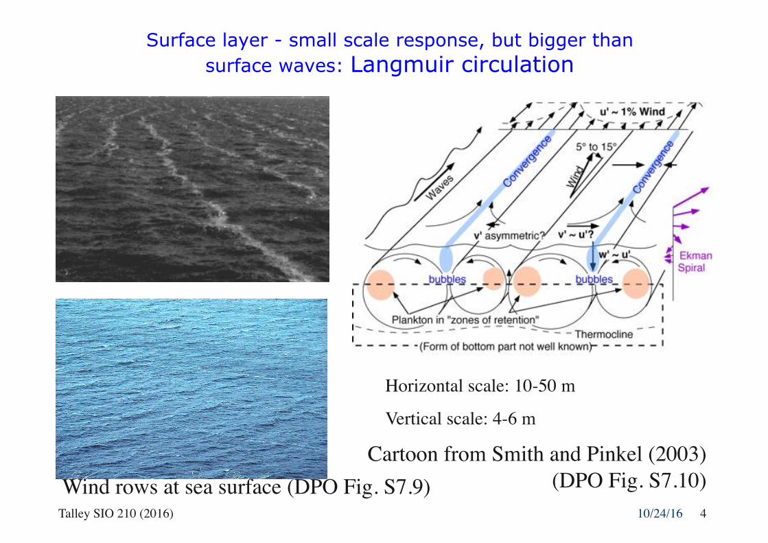
Surface layer - small scale response, but bigger than surface waves: Langmuir circulation

Wind rows at sea surface (DPO Fig. S7.9)

Horizontal scale: 10-50 m

Vertical scale: 4-6 m

Cartoon from Smith and Pinkel (2003) (DPO Fig. S7.10)

Talley SIO 210 (2016) 410/24/16

Surface mixed layer: buoyancy and turbulent mixing effects

Mixing by turbulence only

Mixing by heat loss

Development of mixed layer depends on turbulence input (wind velocity), heat loss or gain (also salt), and pre-existing stratification DPO Fig. 7.3Talley SIO 210 (2016)

510/24/16

Surface mixed layer: maximum mixed layer depth

See also Lecture: Ocean Structure I

DPO Fig. 4.4c from Holte et al al.Talley SIO 210 (2016)6

10/24/16

How does the ocean respond to wind stress at time scales longer than hours?

Talley SIO 210 (2016)7

10/24/16

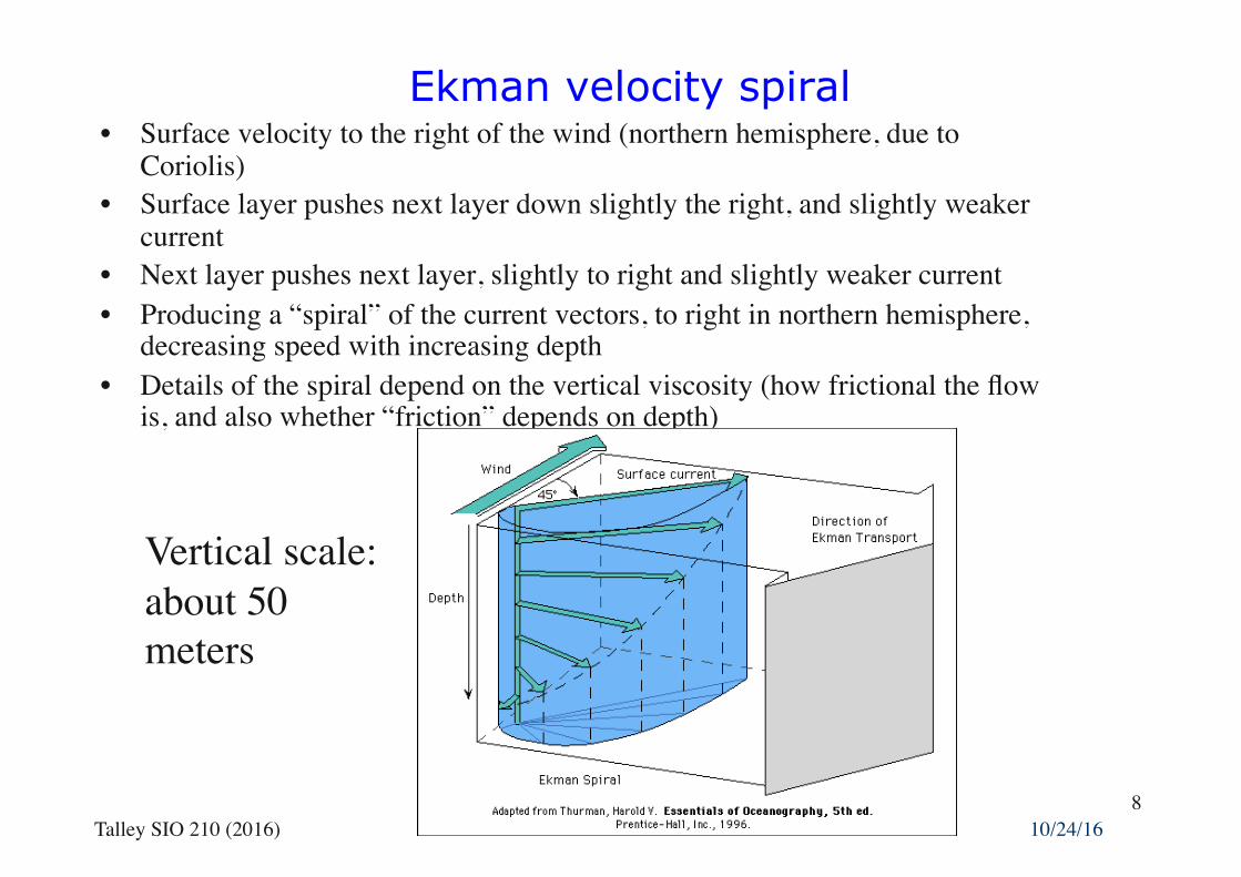
Ekman velocity spiral •  Surface velocity to the right of the wind (northern hemisphere, due to

Coriolis)•  Surface layer pushes next layer down slightly the right, and slightly weaker

current•  Next layer pushes next layer, slightly to right and slightly weaker current•  Producing a “spiral” of the current vectors, to right in northern hemisphere,

decreasing speed with increasing depth•  Details of the spiral depend on the vertical viscosity (how frictional the flow

is, and also whether “friction” depends on depth)

Vertical scale: about 50 meters

Talley SIO 210 (2016)8

10/24/16

Complete force balance with rotation

Three equations:

Horizontal (x) (west-east) acceleration + advection + Coriolis = pressure gradient force + viscous term

Horizontal (y) (south-north) acceleration + advection + Coriolis = pressure gradient force + viscous term

Vertical (z) (down-up) acceleration +advection (+ neglected very small Coriolis) = pressure gradient force + effective gravity

(including centrifugal force) + viscous term

Inertial motionGeostrophic flow

Talley SIO 210 (2016)

Ekman balance

910/24/16

Final equations of motion (momentum equations in Cartesian coordinates)

x: ∂u/∂t + u ∂u/∂x + v ∂u/∂y + w ∂u/∂z - fv = - (1/ρ)∂p/∂x + ∂/∂x(AH∂u/∂x) + ∂/∂y(AH∂u/∂y) +∂/∂z(AV∂u/∂z) (7.11a)

y: ∂v/∂t + u ∂v/∂x + v ∂v/∂y + w ∂v/∂z + fu = - (1/ρ)∂p/∂y + ∂/∂x(AH∂v/∂x) + ∂/∂y(AH∂v/∂y) +∂/∂z(AV∂v/∂z) (7.11b)

z: ∂w/∂t + u ∂w/∂x + v ∂w/∂y + w ∂w/∂z (+ neglected small Coriolis) = - (1/ρ)∂p/∂z - g + ∂/∂x(AH∂w/∂x) + ∂/∂y(AH∂w/∂y) +∂/∂z(AV∂w/∂z) (7.11c)

Talley SIO 210 (2016)10

Ekman balance

Hydrostatic (doesn’t figure in)

10/24/16

Equations of motion and frictional balance in an Ekman layer

Three APPROXIMATE equations:

Horizontal (x) (west-east) Coriolis = vertical viscosity

Horizontal (y) (south-north) Coriolis = vertical viscosity

Vertical (z) (down-up) (hydrostatic balance) 0 = pressure gradient force + effective gravity

NOTE: NO HORIZONTAL PRESSURE GRADIENT FORCE OR ACCELERATION in an Ekman layer

That is: x: -fv = ∂/∂z(AV∂u/∂z)

y: fu = ∂/∂z(AV∂v/∂z)Talley SIO 210 (2016)

1110/24/16

Ekman transport The wind stress on the ocean surface is the vector

τ = ( τ(x) , τ(y) )

Integrate the Coriolis/friction balances in the vertical

x: -fv = ∂/∂z(AV∂u/∂z) -> -fVEK= AV∂u/∂z = τ(x) /ρ y: fu = ∂/∂z(AV∂v/∂z) -> fUEK= AV∂v/∂z = τ(y) /ρ

• UEK and VEK are the “Ekman transport” ∫udz, ∫vdz

• Ekman “transport” is exactly to the right of the wind stress (northern hemisphere ) (to left of wind stress in southern hemisphere since f has the opposite sign).

• Ekman transport does not depend on the size or structure of AV (but the detailed structure of the spiral DOES depend on it)

Talley SIO 210 (2016)12

10/24/16

Ekman layer “transport” •  “Transport”: 90° to wind, to right in NH and left in SH •  UEk= τ/ρf (units are m2/s, not m3/s so technically this is not a

transport; need to sum horizontally along a section to get a transport).

•  Typical size: for wind stress 0.1 N/m2, UEk= 1 m2/s. Integrate over width of ocean, say 5000 km, get total transport of 5 x 106 m3/sec = 5 Sv.

Talley SIO 210 (2016)13

10/24/16

Ekman layer depth

•  Depth: depends on eddy viscosity AV (why?) Dek = (2AV/f)1/2

•  Eddy viscosity AV is about 0.05 m2/sec in turbulent surface layer, so Ekman layer depth is 20 to 60 m for latitudes 80° to 10°.

Talley SIO 210 (2016)14

10/24/16

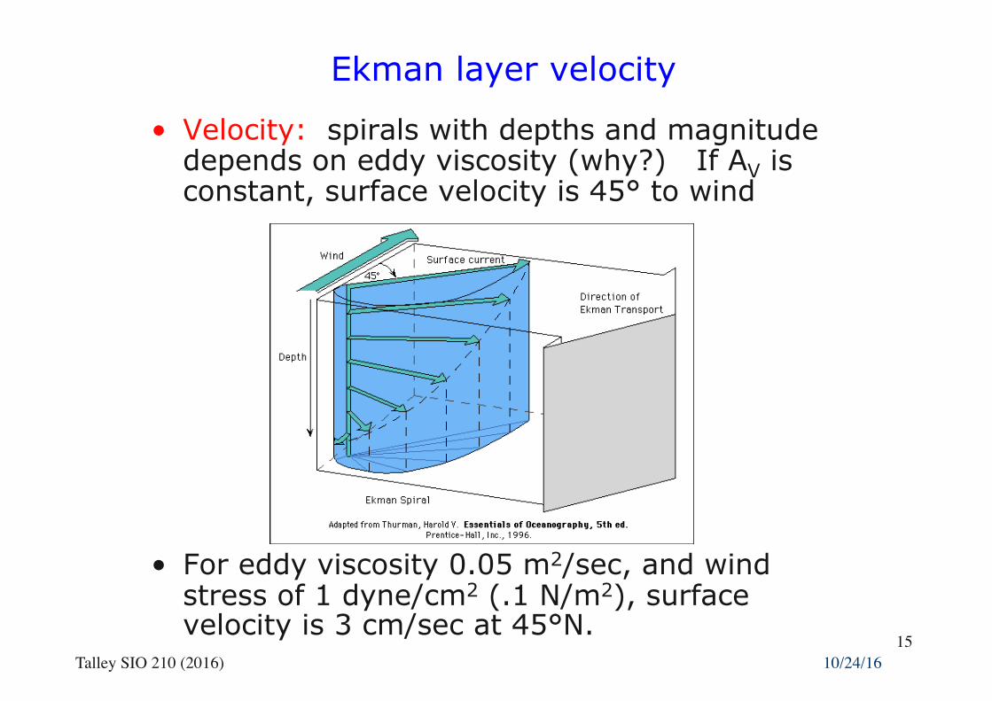
Ekman layer velocity

•  Velocity: spirals with depths and magnitude depends on eddy viscosity (why?) If AV is constant, surface velocity is 45° to wind

•  For eddy viscosity 0.05 m2/sec, and wind stress of 1 dyne/cm2 (.1 N/m2), surface velocity is 3 cm/sec at 45°N.

Talley SIO 210 (2016)15

10/24/16

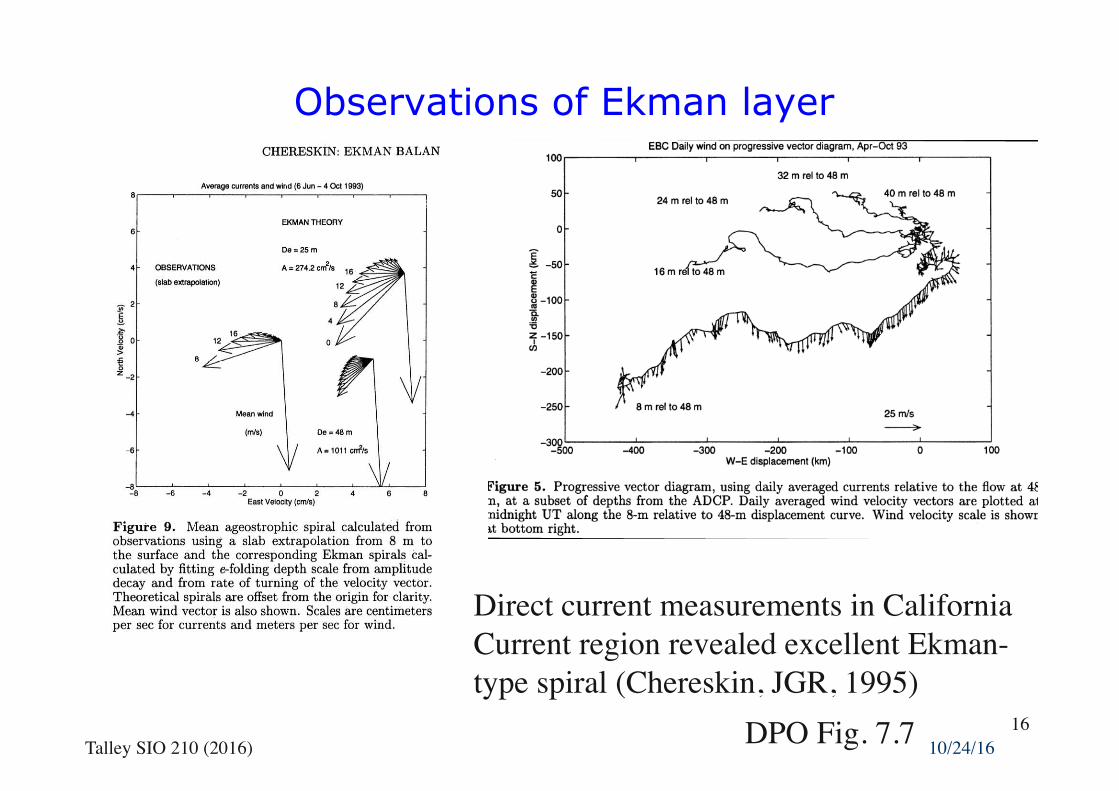
Observations of Ekman layer

Direct current measurements in California Current region revealed excellent Ekman-type spiral (Chereskin, JGR, 1995)

DPO Fig. 7.7Talley SIO 210 (2016)16

10/24/16

Basinwide demonstration of Ekman balance using surface drifters (Ralph and Niiler, 1999)

Blue - average wind

Red - average 15 meter current

DPO Fig. 7.8

Talley SIO 210 (2016)17

10/24/16

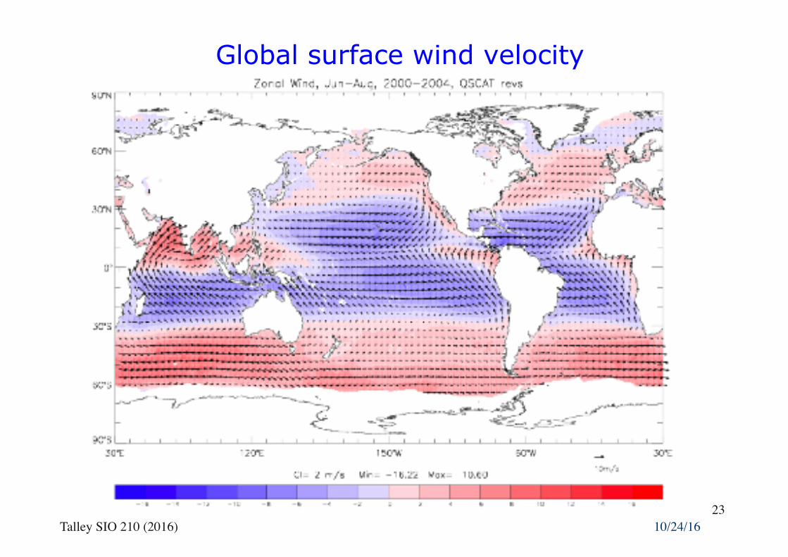
Global surface wind velocity

Talley SIO 210 (2016)18

10/24/16

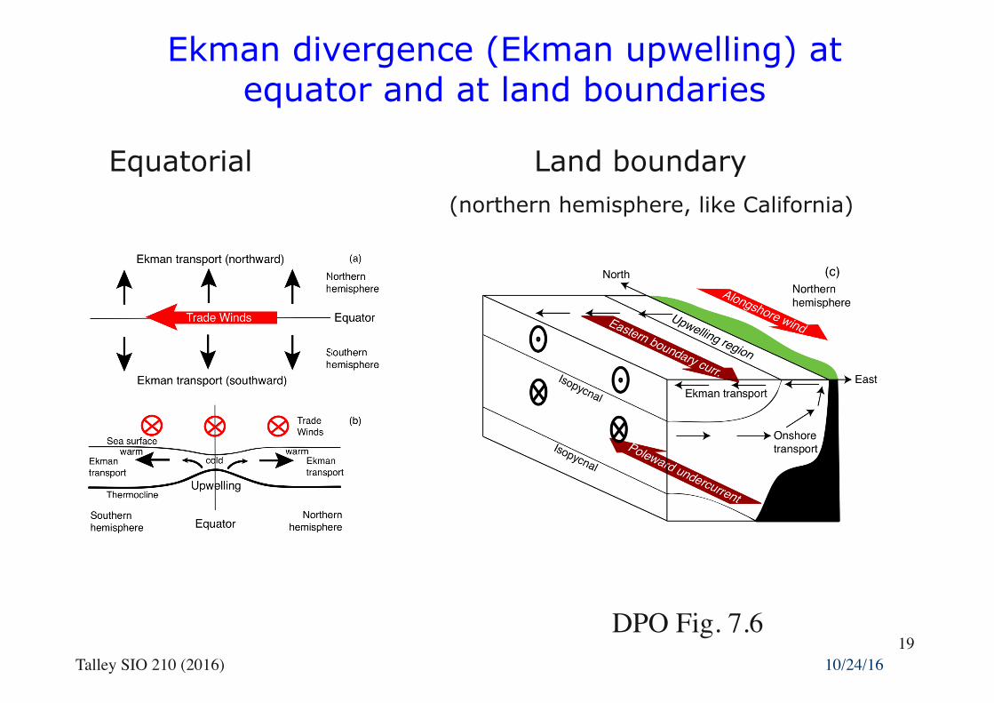
Ekman divergence (Ekman upwelling) at equator and at land boundaries

DPO Fig. 7.6

Equatorial Land boundary (northern hemisphere, like California)

Talley SIO 210 (2016)19

10/24/16

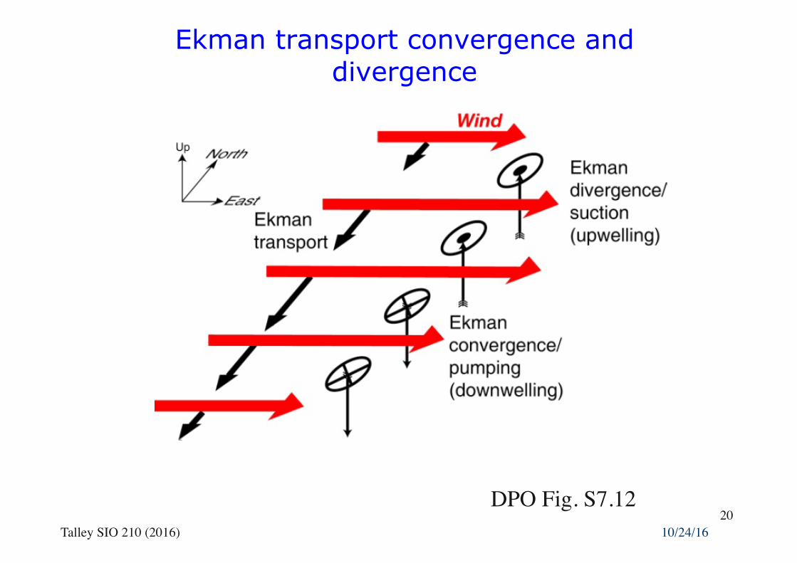
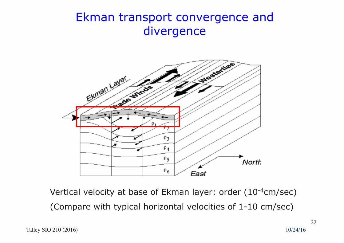
Ekman transport convergence and divergence

DPO Fig. S7.12 Talley SIO 210 (2016)

2010/24/16

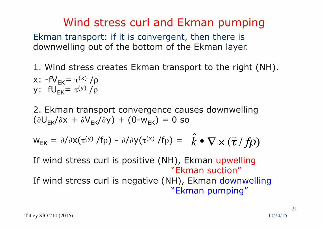
Wind stress curl and Ekman pumping Ekman transport: if it is convergent, then there is downwelling out of the bottom of the Ekman layer.

1. Wind stress creates Ekman transport to the right (NH). x: -fVEK= τ(x) /ρ y: fUEK= τ(y) /ρ

2. Ekman transport convergence causes downwelling (∂UEK/∂x + ∂VEK/∂y) + (0-wEK) = 0 so

wEK = ∂/∂x(τ(y) /fρ) - ∂/∂y(τ(x) /fρ) =

If wind stress curl is positive (NH), Ekman upwelling “Ekman suction”

If wind stress curl is negative (NH), Ekman downwelling “Ekman pumping”

€

ˆ k •∇ × (! τ / fρ)

Talley SIO 210 (2016)21

10/24/16

Ekman transport convergence and divergence

Vertical velocity at base of Ekman layer: order (10-4cm/sec)

(Compare with typical horizontal velocities of 1-10 cm/sec)

Talley SIO 210 (2016)22

10/24/16

Global surface wind velocity

Talley SIO 210 (2016)23

10/24/16

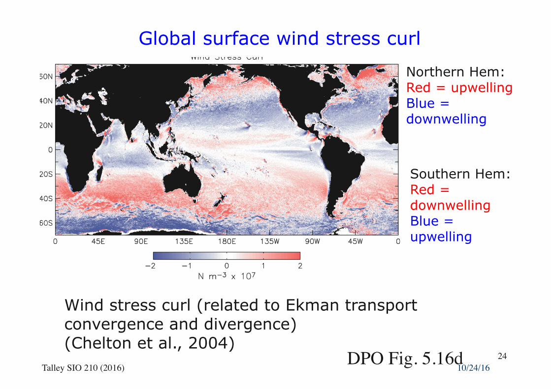
Global surface wind stress curl

DPO Fig. 5.16d

Wind stress curl (related to Ekman transport convergence and divergence) (Chelton et al., 2004)

Northern Hem: Red = upwelling Blue = downwelling

Southern Hem: Red = downwelling Blue = upwelling

Talley SIO 210 (2016)24

10/24/16

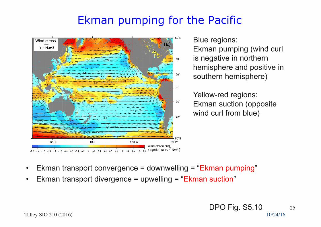
Ekman pumping for the Pacific

•  Ekman transport convergence = downwelling = “Ekman pumping” •  Ekman transport divergence = upwelling = “Ekman suction”

DPO Fig. S5.10

Blue regions: Ekman pumping (wind curl is negative in northern hemisphere and positive in southern hemisphere)

Yellow-red regions: Ekman suction (opposite wind curl from blue)

Talley SIO 210 (2016)25

10/24/16

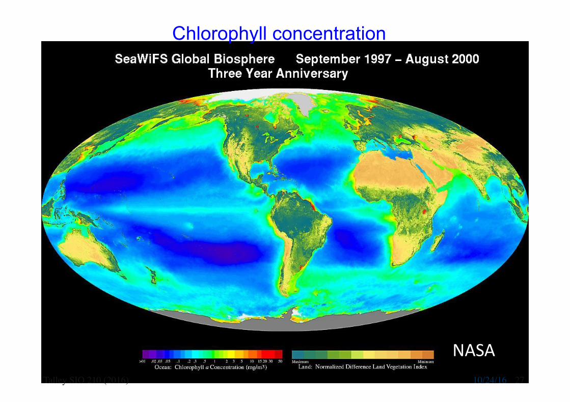
Evidence of Ekman upwelling: surface nitrate concentration

Data from gridded climatology, NODC (Levitus and Boyer, 1994)

DPO Fig. 4.23 Talley SIO 210 (2016)

2610/24/16

NASA  Talley SIO 210 (2016) 2710/24/16

Chlorophyll concentration