43
Operating Instructions easyScan E-AFM (Version 1.0)

1
Operating Instructions
easyScan E-AFM(Version 1.0)

2
‘NANOSURF’ AND THE NANOSURF LOGO ARE TRADEMARKS OF NANOSURF AG, REGISTERED AND/OR
OTHERWISE PROTECTED IN VARIOUS COUNTRIES.© AUGUST 2003 BY NANOSURF AG, SWITZERLAND, R0.2
TEXT & LAYOUT: ROBERT SUM, PIETER VAN SCHENDEL
ENGLISH: VICKI CONNOLLY

3
Table of contents
Introduction 5What is AFM? ....................................................................................... 5Scanning with the ‘easyScan E-AFM’ ................................................... 6
(Un)packing and Installation 9Unpacking the instrument ................................................................... 10Storing the Instrument ........................................................................ 12Hardware installation .......................................................................... 12Software installation ............................................................................ 14
System requirements 14Installation Procedure 15Simulated microscope 17
Preparing for Measurement 18Installing the sensor ............................................................................ 18
Selecting a sensor 18Inserting the sensor in the scan head 19
Installing the sample ........................................................................... 21Preparing the Sample 21Stand-alone measurements 22The small sample stage 23
A First Measurement 24Starting the microscope ...................................................................... 24Approaching the sample ..................................................................... 26
1. Coarse approach by hand 262. Fine approach by linear motor 273. Automatic final approach 28
Starting a measurement ..................................................................... 29Adjusting the measurement plane ...................................................... 30Optimising resolution .......................................................................... 32 Snapshots of images ......................................................................... 35Judging the quality of the images ....................................................... 36Finish measuring ................................................................................ 37
Maintenance 38Scan head 38Scan electronics 38

4
Problems and Solutions 39Sensor Fail LED 39Image quality suddenly deteriorates 39‘No connection to microscope!’ 40
Technical Data 41

5
Introduction
This manual gives instructions on how to set up and use your easyScan E-AFM system. This introduction chapter gives some general information onthe atomic force microscopy technique, and its implementation in the easy-Scan E-AFM. The next chapter, (Un)packing and Installation, should beread when installing your easyScan system. The chapters Preparing for Meas-urement and A First Measurement should be read by all users, because theycontain useful instructions for everyday measurements. The other chaptersgive more information for advanced users. Those who need a more detaileddescription of the functions of the easyScan software should refer to theSoftware Reference manual.
What is AFM?Microscopy is one of the most exciting scientific techniques. The insightinto small dimensions has led to a new understanding of the structure ofmaterials and forms of life.
With the invention of the scanning tunnelling microscope (STM) in theearly eighties it became possible to look into the fascinating world of atoms.The STM was developed by Gerd Binnig and Heinrich Rohrer in the early80’s at the IBM research laboratory in Rüschlikon, Switzerland. For thisrevolutionary innovation Binnig and Rohrer were awarded the Nobel prizein Physics of 1986.
However, the STM technique is restricted to electrically conducting sur-faces. A further development of the STM called the Atomic Force Micro-scope (AFM) was developed by Gerd Binnig, Calvin Quate and ChristophGerber. The AFM extended the abilities of the STM to include insulatingmaterial. Both the AFM and the STM microscopy techniques works with-out optical focusing elements. Instead, a small sharp probing tip is scannedvery closely across the sample’s surface. The distance between the tip andthe sample surface is so small, that atomic-range forces act between them.The tip is attached to the end of a cantilever in order to measure theseforces. The force acting on the tip can then be determined by detecting thedeflection of this cantilever.
INTRODUCTIONWHAT IS AFM?

6
The measurement of the cantilever deflection can be used to control thetip-surface distance on an atomic scale. Thus, enormous resolution can beachieved, such that even atomic arrangements of surfaces can be ‘probed’.This measurement is a so-called static measurement mode, in which thestatic deflection of the cantilever is used.
However, to achieve atomic resolution, ultra-clean and flat surfaces pre-pared in highly sophisticated vacuum systems are needed . Nevertheless,measurements in air can though give useful results for many technicallyrelevant surfaces. In this manual, the use of the dynamic modes in air, ontechnically such surfaces will be described.
Scanning with the ‘easyScan E-AFM’The easyScan E-line atomic force microscope (E-AFM) can be used in thestatic force (contact) operating mode. The AFM sensor is a microfabricatedcantilever with an integrated tip mounted on a sensor holder chip (see fig-ure Cantilever).
When the sensor tip comes in contact with the sample, a repulsive force actson it, that increases with decreasing tip-sample distance. In the static forceoperating mode, the cantilever bending due to the force acting on the tip ismeasured using a laser beam deflection system.
easyScanelectronics
E-AFM system: Computer, Cantilever with deflection measurement system scanning the sample.
INTRODUCTION SCANNING WITH THE ‘EASYSCAN E-AFM’

7
Cantilever: microfabricated silicon cantilever with integrated tip, 450 µm long, 50 µmwide.
The measured laser beam deflection can now be used as an input for afeedback loop that keeps the tip-sample interaction constant by changingthe tip height. The output of this feedback loop thus corresponds to thelocal sample height.
x
y
Scanner coordinate system
An image of the surface is made by recording the sample height as the tip isscanned over the sample surface in the x and y direction. The direction ofthe x- and y-axes of the scanner is shown in the figure Scanner coordinatesystem. The scanner axes may not be the same as the measurement axes,
INTRODUCTIONSCANNING WITH THE ‘EASYSCAN E-AFM’
8
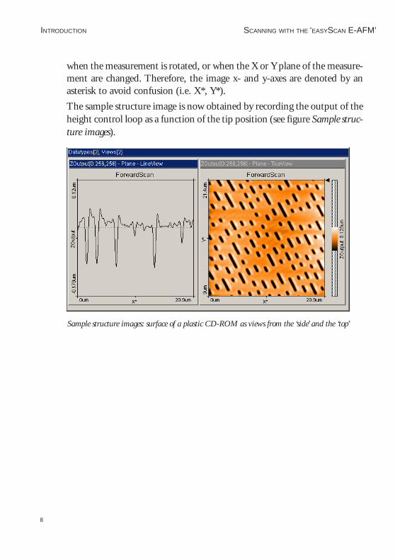
when the measurement is rotated, or when the X or Y plane of the measure-ment are changed. Therefore, the image x- and y-axes are denoted by anasterisk to avoid confusion (i.e. X*, Y*).
The sample structure image is now obtained by recording the output of theheight control loop as a function of the tip position (see figure Sample struc-ture images).
Sample structure images: surface of a plastic CD-ROM as views from the ‘side’ and the ‘top’
INTRODUCTION SCANNING WITH THE ‘EASYSCAN E-AFM’

9
(Un)packing and Installation
The following sections describe the installation of the easyScan E-AFM.
Important!
To make high quality measurements, the following precautions must betaken to keep equipment clean:
• Never touch the sensor tips, the cantilevers (figure Components, 11 d), orthe open part of the scan head (figure Components, 3).
• Ensure that the surface to be measured is free of dust and possible residues.
• Note that the scan head is fixed onto the small-sample stage by threelevelling screws (figure Scan head mounting, left). ALWAYS secure thescan head in this way for transportation or storage.
Scan head mounting: left: transport position - right: operating position
(UN)PACKING AND INSTALLATION

10
Unpacking the instrumentBefore unpacking the instrument suitcase, check for the following items:
13
1
Documents and software (12)
11
87
65
4
2
h
103
9
gi
a
c de
b
f
Components: The easyScan E-AFM system
The easyScan E-AFM system consists of the following components:
1 - easyScan E-SPM electronics
2 - E-AFM Drive electronics
3 - E-AFM scan head
4 - Power supply LPS-1
5 - RS232 cable, connects the easyScan SPM electronics to the computer’sserial port
(UN)PACKING AND INSTALLATION UNPACKING THE INSTRUMENT

11
6 - Mains cable
7 - Cable, connects the easyScan SPM electronics to the E-AFM Drive
8 - Helix cable, connects the E-AFM scan head to the E-AFM Drive
9 - Small sample stage
10 - HeadGuard
11 - E-AFM tool set containing:
a: Sample holder
b: 2 Samples (CD-ROM piece, Microstructure)
c: screwdriver
d: Set of 10 sensors, type CONTR
e: tweezers
f: DropStop
g: sensor insertion tool
h: Allen key
i: Protection feet. The sensor insertion tool is normally mounted insidethe DropStop.
12 - Software installation CD containing easyScan E-Line software, a cali-bration file, E-AFM Operating Instructions (this manual), easyScan E-Line software reference
- A calibration certificate for your E-AFM scan head and electronics
13 - Instrument case
In addition, a computer is needed that meets the requirements described inthe section Software Installation.
Storing the InstrumentIf you have to send in the instrument, transport it or if you are not using itfor some time, please pack it in the instrument suitcase. Then the instru-ment is protected from dust, and the rubber feet of the sample stage (vibra-tion isolation) are relieved.
(UN)PACKING AND INSTALLATIONSTORING THE INSTRUMENT

12
- Turn off the instrument as described in the section finish measuring, andremove all cables in the opposite order as they were mounted.
- Fix the microscope in the transport position and fix the HeadGuard withits two screws (see figure Scan head mounting).
- Pack all components as shown in figure Components.
Important!
For transport, always secure the microscope to the small sample stage, andput it in the original Nanosurf case.
Hardware installation
Important!
- Please check that your local mains voltage corresponds to that of the powersupply (figure Components, 4).
- Make sure that your mains connection is protected against excess voltagesurges.
- Choose a steady table where you can work undisturbed. To ensure thefaultless operation of the E-AFM it has to be isolated from vibrations,heat emission and air current. We also recommend covering the instru-ment with a box to shield it from ‘near infrared’ light from artificial lightsources, because this light may cause noise in the cantilever deflectiondetection system. If the vibration isolation of your table is insufficient foryour measurement purposes, an optional active vibration isolation tableis available.
- Keep the E-AFM scan head (figure Components, 3) in the transport posi-tion (figure Scan head mounting: left) on the small sample stage (whenusing small sized samples) (9). Fix the helix cable (8) to the plug using thescrewdriver (11 c). The helix cable is used to isolate the scan head fromvibrations of the table it is standing on. Take care that it is lying loosely onthe table to ensure proper operation, and avoid stretching it.
- Connect the helix cable (8) to the E-AFM Drive electronics (2).
(UN)PACKING AND INSTALLATION HARDWARE INSTALLATION
13
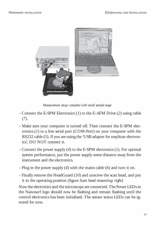
Measurement setup: complete with small sample stage
- Connect the E-SPM Electronics (1) to the E-AFM Drive (2) using cable(7).
- Make sure your computer is turned off. Then connect the E-SPM elec-tronics (1) to a free serial port (COM-Port) on your computer with theRS232 cable (5). If you are using the ‘USB adapter for easyScan electron-ics’, DO NOT connect it.
- Connect the power supply (4) to the E-SPM electronics (1). For optimalsystem performance, put the power supply some distance away from theinstrument and the electronics.
- Plug in the power supply (4) with the mains cable (6) and turn it on.
- Finally remove the HeadGuard (10) and unscrew the scan head, and putit in the operating position (figure Scan head mounting: right)
Now the electronics and the microscope are connected. The Power LEDs inthe Nanosurf logo should now be flashing and remain flashing until thecontrol electronics has been initialized. The sensor status LEDs can be ig-nored for now.
(UN)PACKING AND INSTALLATIONHARDWARE INSTALLATION
14
Warning !This product contains a
Class 1 LaserInvisible laser radiation !
The laser is located behind the sensor.
Although the optical power should do no damage when the instrument isassembled, avoid looking directly into the laser beam.
Laser source information:
Wavelength: 830nm
Optical power: <0.4mW
Class one Laser
Software installation
System requirementsThe System requirements for the easyScan E-Line software are:
• PC with a Pentium 133MHz processor or higher
• a free COM-Port or USB port.*
• Windows 95 or higher
• 8MB RAM or more (16MB recommended)
• graphics adapter with 800 x 600 resolution and 16-bit colours (‘highcolor’) or better (resolution of 1024 x 768 recommended)
* The Nanosurf ‘USB Adapter for easyScan’ option must be acquired touse the USB port.
Installation Procedure
- Turn on your computer and start Windows.
Do not run any other program while installing the scan software.
(UN)PACKING AND INSTALLATION SOFTWARE INSTALLATION

15
- If you want to use the USB Adapter for easyScan, install it first followingthe instructions included with the adapter.
- Insert (the backup copy of ) your E-Line CD.
Windows NT/2000/XP
- Make sure you have administrator privileges before installing the soft-ware.
All operating systems
- Start the ‘setup.exe’ program on the CD, the following screen will nowappear:
- Select the button ‘Install’, to install the data acquisition program ‘easy-Scan’ on your computer.
(UN)PACKING AND INSTALLATIONSOFTWARE INSTALLATION

16
Setup will ask for the directory in which the program files are to be copied:
- Put them in the proposed directory, unless the ‘Program Files’ directoryhas a different name in your language of the Windows operating system.
Afterwards setup will ask for the start menu entry or program group inwhich ‘easyScan’ is to be placed:
- Accept the proposed name by clicking ‘OK’ or type another name.
The installation setup will now ask for the ’COM-Port’:
- Select the serial port to which you have connected the E-SPM electronics(See section hardware installation)
The setup program will start copying files onto your hard-disk.
After successful installation you will get this confirmation:
(UN)PACKING AND INSTALLATION SOFTWARE INSTALLATION

17
Important!
The E-Line software CD delivered with the instrument contains calibra-tion information specific to your instrument, therefore you should keep (abackup copy of ) the CD delivered with the instrument.
Simulated microscopeYou can start the easyScan software without having the microscope con-nected to your computer. We recommend using this simulation to explorethe easyScan-system (measurements and software) ‘off-line’.
When the simulate microscope mode is started, the following dialog boxappears:
By clicking ‘Start Simulation’ a simulation of the microscope is started.This imitates most of the functions of the real microscope. The sample isreplaced by a mathematical description of a surface. You can now follow theinstructions in the chapter A first measurement.
- To explore the system in the ‘Simulate Microscope’ mode with the micro-scope connected, activate it in the menu ‘Options’.
(UN)PACKING AND INSTALLATIONSOFTWARE INSTALLATION

18
Preparing for Measurement
This chapter describes actions that you perform on a day-to-day basis as apreparation for your measurements. These steps are changing the sensor,selecting a sample stage, and preparing the sample.
Installing the sensorTo maximise ease of use, the Nanosurf E-AFM is designed so that the sen-sor can be installed and removed without having to readjust the cantileverdeflection detection system. This is possible because an alignment system isused that consists of an alignment chip and matching grooves in the backside of the sensor. This positions the sensor with micrometer accuracy (seefigure Sensor, Left). Note though, that this accuracy is only guaranteed whenthe sensor and the mounting chip are absolutely clean. Installation of thesensor should therefore still be carried out with great care because goodresults are strongly dependant on the accuracy of this process.
Important!
• Nothing should ever touch the sensor, especially the tip end!
• The sensor holder spring in the open part of the scan head (see figuremounting the sensor) is very delicate and should not be bent!
Selecting a sensorThe sensor should have the following properties:
• The bottom of the sensor chip must have grooves that fit into the align-ment chip.
• The cantilever should have a nominal length of 225 µm or more, and awidth of 40 µm or more.
• The backside of the cantilever must have a reflective coating. Uncoatedcantilevers transmit much of the infrared light of the deflection detectionsystem.
Presently, only sensors from the companies NanoWorld and NanoSensorscan be used. Type CONTR and ZEILR sensors can be used.
PREPARING FOR MEASUREMENT INSTALLING THE SENSOR

19
Sensor: Left: Sensor alignment system, Right: Sensor chip viewed from the top.
Inserting the sensor in the scan head
1. Turn the scan-head upside-down.
2. Take the DropStop (figure Contents, 11 f), and remove the sensor inser-tion tool. Gently snap the DropStop over the scan head (see drawingInstalling the DropStop).
Installing the DropStop
3. Plug the sensor insertion tool (Components, 11 g) into the hole behind thesensor holder (figure mounting the sensor, top right). The sensor holderflap opens.
4. Use the tweezers to take the sensor out of its box. The sensor is noworiented face up.
5. Let the sensor carefully slide into the silver alignment chip in the scanhead. Make sure the sensor lies precisely in the alignment chip (figuremounting the sensor, bottom left).
PREPARING FOR MEASUREMENTINSTALLING THE SENSOR

20
Mounting the sensor: top left: The sensor holder spring, top right: Plugging in the sensor insertiontool, bottom left: inserting the sensor. Bottom right: a correctly built in sensor.
6. GENTLY pull the sensor insertion tool out of the hole; the sensor holderflap closes and holds the sensor chip tightly (figure mounting the sensor,bottom right).
7. Remove the DropStop from the scan head. Please note that the laserbeam is blocked by the DropStop as long as it is in place. The sensorLED on the E-AFM Drive only displays the actual status of the sensorafter removing the DropStop .
8. The green ‘OK’ sensor control LED on the E-AFM Drive electronicsshould now be on. If this is not the case refer to Chapter Problems andSolutions.
PREPARING FOR MEASUREMENT INSTALLING THE SENSOR

21
Sensor status LEDs
Installing the sample
Preparing the SampleThe E-AFM can be used to examine any material with a surface roughnessthat does not exceed the height range of the scanning tip. Nevertheless thechoice and preparation of the surface can influence the surface-tip interaction.Examples of influencing factors are excess moisture, dust, grease etc. Be-cause of this some of the samples need special preparation to clean its sur-face. Generally, clean as little as possible.
If the surface is dusty, try to measure on a clean area between the dust. It ispossible to blow coarse particles away with dry, oil free air, but small parti-cles generally stick so well to the surface, that they can not be removed.Note that bottled pressurized air is generally dry, but pressurised air froman in-house supply is generally not. In this case an oil filter should be in-stalled. Blowing dust away by breath is not advisable, because it is not dry.
If surface contaminants, such as grease or oil are present, the surface shouldbe cleaned with a solvent. Suitable solvents are distilled or demineralisedwater, alcohol or acetone, depending on the contaminant. The solvent shouldbe very pure, in order to prevent the collection of impurities on the surfacewhen the solvent evaporates. The sample should be cleaned several times toremove dissolved and redeposited contaminants if it is very contaminated.Delicate samples can be cleaned in an ultrasound bath.
PREPARING FOR MEASUREMENTINSTALLING THE SAMPLE

Standard samples
The Microstructure sample supplied with the instrument (figure Compo-nents, 11 b) is meant as a test sample. It can be used to check the correctnessof the instrument calibration. The grid is manufactured using a standardsilicon process that creates square holes in a silicon oxide layer on a siliconsubstrate. The grid period is 10 µm for the large scan heads, the depth of theholes is approximately 100 nm. The exact period and height (with 3 %accuracy) are given on the box. Certified XYZ calibration grids are availableas an option.
The CD-ROM piece is a part of a stamped CD-ROM on which no reflec-tive and protective coatings have been deposited. This allows you to meas-ure the pits that have been stamped in the CD.
Both sample should be kept in their boxes. Then it should be unnecessaryto clean them. Cleaning is not advisable, because the samples are ratherdelicate.
Stand-alone measurementsYou can either use the instrument with the supplied small-sample stage, oras a stand-alone instrument. Use the small-sample stage if possible, andlimit the stand-alone operation to samples that are too large. For stand-alone measurements, the scan head itself can be put directly on top of thesample. Small plastic protection feet for under the three metal feet are pro-vided to protect delicate samples from scratching (figure components, 11 i).
E-AFM used as Stand-Alone instrument
PREPARING FOR MEASUREMENT INSTALLING THE SAMPLE

The small sample stageThe small-sample stage can be used to comfortably position the sample. Anx-y positioning table with micrometer screws is available as an option.
Small-Sample Stage
- Mount the small sample onto the sample holder. The simplest way to dothis is to use put the sample on the sticky side of a Post-it® note that isattached to the sample holder using double sided adhesive tape. It is ad-vantageous to measure the standard samples using the small sample stage,because it allows better positioning.
Sample mounted onto the sample holder
Important!
Avoid all mechanical impact on the sensor when placing the sample holderunder the scan head. Any impact will damage the tip.
PREPARING FOR MEASUREMENTINSTALLING THE SAMPLE

24
A First Measurement
Preparations are now complete: The instrument has been assembled andthe software installed. A static force mode sensor and the microstructuresample (figure Components, 11 b) are ready for measurement.
In this chapter, step by step instructions are given as to how to operate themicroscope and get your first pictures. More detailed explanations for thesoftware and the system are given in the software reference manual.
Important!
• Never touch the sensor or the surface of the sample ! Good results relyheavily on the accuracy of the preparation of the tip and the sample.
• Avoid exposing the system to direct light during measuring. This couldinfluence the sensor unit and deteriorate the quality of the measurement.
Starting the microscope
- Check that the power supply (4) is connected to the AC mains powersupply, and that the power supply is on.
The red LEDs of the control electronics (2, 3) are flashing and the green‘Sensor OK’ LED is shining.
- Start the ‘easyScan E-Line’ software on your computer.
The main program window and a message box appear:
Now, your computer is communicating with the control electronics to ini-tialise the system. This process is repeated every time the control electronicsis turned off and on again. When download is completed, the electronic’sred LEDs change from flashing to constantly shining, some control panelsappear (see figure Main program window).
A FIRST MEASUREMENT STARTING THE MICROSCOPE

25
Main program window
Check that the spring constant corresponds to that of your cantilever:
- Open the Sensor Configuration dialog via the menu ‘Options/Config.Sensor’
- Enter the correct spring constant. The value is approximately 0.2 forCONTR cantilevers, the exact value is sometimes given on a separatepiece of paper delivered with the sensors.
A FIRST MEASUREMENTSTARTING THE MICROSCOPE

26
Approaching the sampleTo start measuring, the sensor’s tip must come within a fraction of a nano-meter of the sample, without touching it with to much force. To achievethis, a very careful and sensitive approach of the sensor is required. Thisdelicate operation is carried out in three steps: Coarse approach by hand,fine approach by motor, and the automatic final approach.
If the sample is reflective, the different stages of the approach are best ob-served using the side view of the integrated optics of the scan head (figureIntegrated optics, right). You can use the cantilever as a ‘yardstick’ to judgedistances in the views of the integrated optics.
Integrated optics: left: view through the magnifier from top, right: side view
An optional video camera is available, that allows you to see both viewsfrom your chair. This camera is particularly useful when the microscope isin a position that is difficult to reach, or when you do not wish to contami-
nate the sample with dust particles from your body. Click for the top-
view, click for the side view.
1. Coarse approach by hand
- Ensure a large enough distance is available between sensor and samplesurface so as not to break the cantilever off, then push the sample holder(12) carefully under the sensor.
A FIRST MEASUREMENT APPROACHING THE SAMPLE

27
- Use the three levelling screws to lower the scan head so that the sensor iswithin 1-2 mm of the sample. (Figure coarse approach) Take care that allscrews are moved approximately the same distance, so that the scan headremains levelled.
Coarse approach with the levelling screws
When the sample is reflective, the mirror image of the cantilever should bevisible in the side view of the integrated optics. When the sample is notreflective, the shadow of the cantilever may be visible. If neither a mirrorimage nor a shadow are visible, change the lighting conditions until it isvisible, for example by changing the illumination, or by shading the lightfrom bright surfaces in the room or outside.
2. Fine approach by linear motor
- Choose the menu ‘Panels’ in the ‘easyScan’ program.
- Open the ‘Approach Panel’.
A FIRST MEASUREMENTAPPROACHING THE SAMPLE

28
- Watch the distance between tip and sample in the side view of the inte-grated optics. Now click and hold in the ‘Approach Panel’ to movethe tip towards the sample, to a distance of a fraction of a millimetre.
The distance between the cantilever and its mirror image should now bearound a cantilever length (depending on the type of cantilever).
3. Automatic final approach
- Open the ‘Feedback Panel’ in the menu ‘Panels’.
- Check that the correct settings are used:
• ‘SetPoint’: 20nN or less.
• ‘P-Gain’, ‘I-Gain’: 10.
When you have to change the instrument settings in any panel, you can usethe following methods to change them:
• Activate any input by clicking in it with the mouse pointer, or by select-ing it with the Tab-key.
• The value of an activated input can be increased and decreased using theup and down arrow keys on the keyboard. The new value is automaticallyused after one second.
• The value of a numerical input can also be increased and decreased byclicking the arrow buttons with the mouse pointer. The new value isautomatically applied after one second.
• The value of an active numerical input can be entered using the key-board. The entered value must be confirmed by pressing the ‘Enter’ or‘Return’ key, or by clicking with the mouse pointer.
A FIRST MEASUREMENT APPROACHING THE SAMPLE

29
• The selection of a drop-down menu (e.g.: ) can be changedusing the mouse. The selected value must be confirmed by pressing the‘Enter’ or ‘Return’ key, or by clicking with the mouse pointer.
- Click in the ‘Approach Panel’.
The sensor holder is now moved towards the sample with the help of alinear motor. The motion continues until the measured signal crosses thethreshold value given in the ‘SetPoint’ input of the feedback panel. Fromnow on the distance between sample and sensor is controlled automaticallyby the electronics. The dialogue box ‘Approach done’ appears when theapproach has been completed.
- Click ‘OK’.
Starting a measurementAfter a successful approach the instrument starts measuring automatically.
In the scan panel enter an image size of about half the maximum scan rangeof your scan head in the ‘scan range’ input.
An image of the measurement will be drawn on your screen, showing a linein the ‘LineView’ and a plane in the ‘TopView’. Watch the displays for awhile until about a quarter of the ‘TopView’-image has been measured.
A ‘nervous’ line in the ‘LineView’ indicates too many vibrations, too muchacoustic noise or direct light shining onto the sensor. This means that youshould stop measuring and reduce or eliminate the disturbances:
- Click and follow the instructions of the chapter Problems and Solu-tions.
When the line in the ‘LineView’ is calm and reproduces consistently youcan continue with the next section.
A FIRST MEASUREMENTSTARTING A MEASUREMENT

30
Adjusting the measurement plane
Unadjusted slope: measurement with improperly set X*-slope
Ideally, the plane of the measurement and the sample surface lie in the x-y-plane of the scanner. But mostly the sample plane is tilted with respect tothat ideal plane, as shown is figure Unadjusted slope. In this case, the samplecross section in the X* measurement direction, as shown in the ‘LineView’window, has a certain slope. This slope depends on the direction of the X*direction and therefore on the rotation of the measurement, as shown infigure Slope, position A and B. The measurement plane should be parallel tothe sample plane, because this makes it easier to see smaller details in themeasurement, and because the z-feedback loop functions more accuratelyin this case. Therefore, the measurement plane should adjusted by properlysetting the values of ‘X-Slope’ and ‘Y-Slope’. It is also possible to align the x-
A FIRST MEASUREMENT ADJUSTING THE MEASUREMENT PLANE

31
y-plane of the scanner with the sample plane using the three coarse ap-proach screws on the scan head, but this should not be done when the tip isapproached to the sample.
Slope: Sample’s and measurement orientation before slope adjustment
You can align the measurement plane using the following procedure:
- Alter the value of ‘X-Slope’ using the arrow buttons until the x-axis of thescan line lies parallel to the x-axis of the sample. You can measure theslope in the LineView using the angle tool (see Software Reference).
- Enter the value 90 in the ‘Rotation’ input to scan along the y-direction ofthe scanner i.e. the sample’s slope as shown in the schematics view B. Ifthe input for ‘Rotation’ is not visible, you can make it visible by clicking
.
- If the scan line is not horizontal, alter the value for ‘Y-slope’ until the y-axis of the scan lies parallel to the y-axis of the sample.
- Reset the ‘Rotation’ to 0°. The ‘LineView’ shows the X-slope again.
A FIRST MEASUREMENTADJUSTING THE MEASUREMENT PLANE

32
The value of the ‘Z-Offset’ varies slightly during measurement. This is cor-rect because the option ‘Auto. Adjust Z-Offset’ in the menu ‘Options’ shouldbe active.
Displays after adjusting the slopes
Optimising resolutionYou have prepared your measurement so that the scan line in the centre ofthe ‘LineView’ reproduces stably. Now the scan range has to be reduced andthe measured signals amplified in order to observe the surface structure.
Reminder: Measurements on the micrometer/nanometer scale are very sen-sitive. Direct light, fast movements causing air flow and temperature varia-tions near the scan head can influence and disturb the measurement.
The following procedure applies to measurements on the Microstructuresample (figure components, 11 b):
A FIRST MEASUREMENT OPTIMISING RESOLUTION

33
1. Reduce the data range by reducing ‘Z-Range’ in the ‘Scan Panel’ to about0.3 µm in order to improve the resolution of the measured data.
Diminishing ‘Z-Range’ amplifies the signal in Z-direction
2. Reduce the scan range as follows:
- click the ‘TopView’-Display to activate it: its title bar should be the samecolour as the title bar of the scan panel.
- click : The mouse pointer becomes a cross and the ‘Tool Info Panel’opens.
- look for an ‘interesting’ region in ‘TopView’ and make a square there withthe mouse pointer. The size of the square is shown in the ‘Tool Info Panel’.
A FIRST MEASUREMENTOPTIMISING RESOLUTION
34
- Release the mouse button when the square’s size is for example about 20µm.
- Confirm the selection by double clicking the display using the left mousebutton. Now the selection is enlarged to the whole display size. You canabort the zoom function by clicking the right mouse button.
3. The best resolution very much depends on the tip-sample conditions(effective tip radius, sample cleanness etc.) In the following, an exampleis given on the XYZ calibration grid to examine the step quality.
- Reduce the Z-range so that the signal displayed in the ‘LineView’ windowdoes not exceed the upper or lower limits. Then lower the scan range tobetween 2-5µm
- Set the values in ‘Scan Panel’ one after the other. Experiment with thesevalues, they can be reduced even further. Between changes always allowthe computer to scan a couple of lines before continuing.
- Pay attention to the height of the signal in the ‘LineView’ window. Itshould not exceed the window height, if it does, the z-Range is too smalland should be increased.
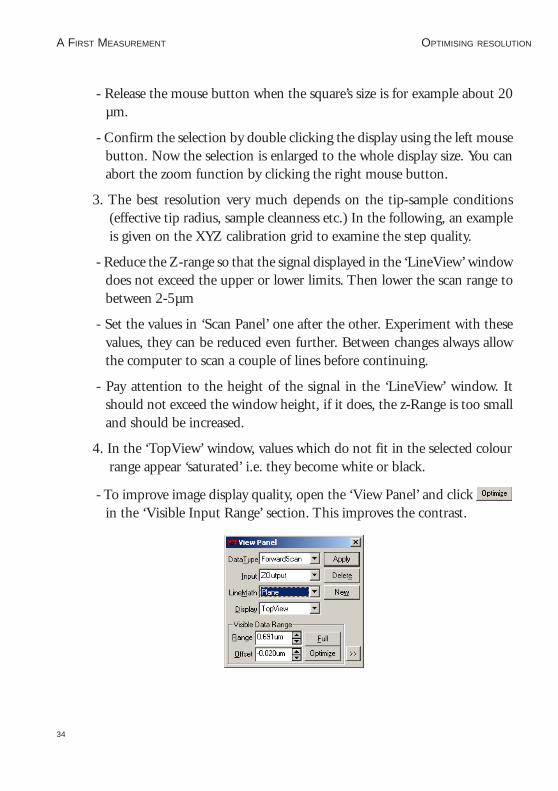
4. In the ‘TopView’ window, values which do not fit in the selected colourrange appear ‘saturated’ i.e. they become white or black.
- To improve image display quality, open the ‘View Panel’ and click in the ‘Visible Input Range’ section. This improves the contrast.
A FIRST MEASUREMENT OPTIMISING RESOLUTION

35
Images of a successful measurement
Snapshots of imagesWhen you are satisfied with your image and would like to keep it, you cantake a snapshot and save it for later:
- During the measurement, you can select in the ‘Scan Panel’. Afterhaving completed the actual frame, a copy of the measured image is takenand displayed in a separate window behind the ‘Scan Panel’.
- If you would like to take the snapshot of the view as it appears during themeasurement without waiting to finish the frame, stop the scanning us-ing and generate a copy of the view using .
After finishing the measurements you can store the ‘photographs’ of yourmeasurements in a storage medium e.g. your PC’s hard drive (see sectionFinish measuring).
A FIRST MEASUREMENT SNAPSHOTS OF IMAGES

36
Judging the quality of the imagesFrom the quality of the measured images the quality of the tip can be ob-served. A good tip quality is necessary for high quality images of high reso-lution.
• When the image quality deteriorates dramatically during a previouslygood measurement, the tip has most probably picked up some particles.
- See section ‘Problems an Solutions: Image quality suddenly deteriorates’
In the following cases the sensor has to be replaced in order to re-establishhigh image quality:
• images in the top view consist of uncorrelated lines only.
• images appear blurred
- First follow the suggestions in section ‘Problems an Solutions: Imagequality suddenly deteriorates’. If these do not help, the cantilever shouldbe changed.
• If all peaks in the image have the same, usually triangular shape, the tip isno longer sharp and has to be replaced. The measured structure is calleda tip artefact.
Image containing tip artifacts
A FIRST MEASUREMENT JUDGING THE QUALITY OF THE IMAGES

37
Finish measuring
- Click to stop measuring.
- You can retract the sensor to a safe and visible distance from the sample byclicking in the ‘Approach Panel’, and afterwards clicking for some time.
- Close all panels in order to see the saved ‘snapshots’.
- Activate the measurement document you would like to save by clicking it.Select the menu ‘File->Save as...’. Select the name and the folder whereyou would like to store the measurement.
These stored measurements can be reload with the ‘easyScan’ software, andthen viewed, analysed and printed (see also Software Reference manual) anytime.
Turning off the instrument
- Exit the ‘easyScan E-Line’ program after having stored all desired images.If you leave the program without saving some data the program asks ifyou wish to save them:
- Turn off the power supply.
If you perform measurements regularly
Leave the instrument and cover the scanner to protect it from dust.
If you do not operate the instrument for several weeks
Put the instrument back into the instrument suitcase. (See also: Storing theInstrument)
A FIRST MEASUREMENTFINISH MEASURING

38
Maintenance
To ensure fault free operation of the microscope the following instructionsfor maintenance have to be followed.
Scan headIt is very important to keep the sample holder and the open part of thescanner clean. If exposed to moisture (high humidity), corrosion will ap-pear.
- Clean the sensor holder adjustment chip by blowing away dust using dry,oil free air.
Scan electronicsClean the case and the controls with a soft cloth lightly moistened with amild detergent solution. Do not use any abrasive pads or solvents like alco-hol or spirits.
MAINTENANCE

39
Problems and Solutions
Sensor Fail LED
• The red ‘Sensor Fail’ LED on the E-AFM Drive electronics can be causedby a misaligned sensor chip.
• Check that the sensor chip is lying perfectly in the alignment chip.
• Remove the sensor using the sensor insertion tool (11 g). Blow awaydust from the alignment chip and the sensor’s back side using dry, oilfree air. Remount the sensor.
Image quality suddenly deteriorates
• When a scan line suddenly starts reproducing badly, the tip may havepicked up some particles:
• Continue measuring for a while (1-2 images), the tip may eventuallyloose these particles again.
• Retract the sensor by clicking then perform a new ap-proach.
• Try to induce changes in the tip’s end: While measuring increase theforce ‘SetPoint’ in the ‘Feedback Panel’. Restore the set point to itsold value when the contrast improves, or nothing happens after scan-ning several lines.
Change the sensor if no improvement can be seen after these procedures.
• If the scan line in the ‘LineView’ suddenly disappears, the tip has lostcontact:
• Increase the value of ‘Z-Range’ in the ‘Scan Panel’
• Increase the force load (Set Point).
• Click in the ‘Approach Panel’ then repeat the steps in chap-ter ‘Start measurement’.
PROBLEMS AND SOLUTIONS

40
‘No connection to microscope!’
This error message appears when the scanning software is waiting for ananswer from scan electronics. This can have various reasons:
• The microscope is not connected:
- If you wish to perform a simulated measurement select .
Otherwise check the connection and select .
• The easyScan SPM electronics is not connected to the power supply:
- check that the power LEDs on the electronics are on.
- check the connection.
• The easyScan SPM electronics is not connected to the computer:
- check the connection.
• The wrong COM-port has been selected during software installation:
- Use , and select the correct COM-port in the dialog:
• The scan electronics is performing a task which lasts an unforeseen lengthof time causing a time-out. Using Windows NT this can happen whenthe system is occupied with itself and blocks the serial port:
- Use .
• The electronics is damaged.
- Contact your dealer.
PROBLEMS AND SOLUTIONS
41
Technical Data
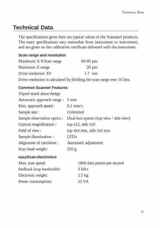
The specifications given here are typical values of the Nanosurf products.The exact specifications vary somewhat from instrument to instrument,and are given on the calibration certificate delivered with the instrument.
Scan range and resolution
Maximum X-Y-Scan range 60-80 µm
Maximum Z-range 20 µm
Drive resolution XY 1.7 nm
Drive resolution is calculated by dividing the scan range over 16 bits.
Common Scanner Features
Tripod stand alone design
Automatic approach range : 5 mm
Max. approach speed : 0.1 mm/s
Sample size : Unlimited
Sample observation optics : Dual lens system (top view / side view)
Optical magnification : top x12, side x10
Field of view : top 4x4 mm, side 3x5 mm
Sample illumination : LEDs
Alignment of cantilever : Automatic adjustment
Scan head weight: 350 g
easyScan electronics
Max. scan speed: 1800 data points per second
feedback loop bandwidth: 3 kHz
Electronic weight: 2.5 kg
Power consumption: 25 VA
TECHNICAL DATA

42
Compatible cantilevers
Manufacturers: NanoSensors, NanoWorld
Static Force Modes: 0.2N/m, Type: CONTR
1.6N/m, Type: ZEILR
Available tips: Standard, SuperSharpSilicon,
HighAspectRatio, Diamond
Typical static load : 10nN
TECHNICAL DATA

43
Am
plifi
er
Lase
r D
rive
1..2
56
-
+A
DC
12B
it
E-A
FM
Sca
n H
ead
E-A
FM
Driv
eea
syS
can
E-L
ine
SP
M E
lect
roni
cs
CP
U
Cus
tom
prog
.Lo
gic
Sca
nZ
-Fee
dbac
kA
ppro
ach
Spe
ctro
scop
y
RS232
Host PC
RAM
ROM
3*16
Bit
DA
C
+-1
0V
+-1
0VS
enso
r S
tatu
s
Opt
iona
l
Opt
iona
l
Cal
ibra
tion
Sta
geS
tatu
s
16B
it D
AC
XYZ - Coil Scanner
Z-Approach
Laser
Can
tilev
er
3*16
Bit
DA
C16
Bit
DA
C+
-12V
Coi
l Driv
esX
/Y/Z
-Axi
s
12 B
it D
AC
+-1
2VA
ppro
ach
spee
d
16 B
it D
AC
+-1
0VG
ap/T
ip V
olta
ge
Set
Poi
nt
Cha
nnel
0
Detector
DC-Motor
AD
C 1
2Bit
Cha
nnel
2
Vid
eo In
Vid
eo o
ut
Vid
eoM
ultip
lexe
r
Hea
d S
tatu
sS
uper
viso
r
Def
lect
ion
Det
ecto
r
Leve
r S
ig
Schematic of the easyScan electronics
TECHNICAL DATA


