arX

iv:1

601.

0776

2v1

[ast

ro-p

h.S

R]

28 J

an 2

016

Astronomy& Astrophysicsmanuscript no. hd5550_v9 c©ESO 2016January 29, 2016

The magnetic field of the double-lined spectroscopic binarysystem HD 5550 ⋆

E. Alecian1, 2, 3, A. Tkachenko4, C. Neiner3, C.P. Folsom1, 2, B. Leroy3, and the BinaMIcS collaboration

1 Univ. Grenoble Alpes, IPAG, F-38000 Grenoble, France2 CNRS, IPAG, F-38000 Grenoble, France3 LESIA, Observatoire de Paris, PSL Research University, CNRS, Sorbonne Universités, UPMC Univ. Paris 06, Univ. Paris Diderot,

Sorbonne Paris Cité, 5 place Jules Janssen, 92195 Meudon, France4 Instituut voor Sterrenkunde, KU Leuven, Celestijnenlaan 200D, 3001 Leuven, Belgium

Received September 15, 1996; accepted March 16, 1997

ABSTRACT

Context. The origin of fossil fields in intermediate- and high-mass stars is poorly understood, as is the interplay between binarityand magnetism during stellar evolution. Thus we have begun astudy of the magnetic properties of a sample of intermediate-mass andmassive short-period binary systems, as a function of binarity properties.Aims. This paper specifically aims to characterise the magnetic field of HD 5550, a double-lined spectroscopic binary system ofintermediate-mass.Methods. We gathered 25 high-resolution spectropolarimetric observations of HD 5550 using the instrument Narval. We first fit theintensity spectra using Zeeman/ATLAS9 LTE synthetic spectra to estimate the effective temperatures, microturbulent velocities, andthe abundances of some elements of both components, as well as the light-ratio of the system. We then applied the multi-line least-square deconvolution (LSD) technique to the intensity and circularly polarised spectra, which provided us with mean LSD I andVline profiles. We fit the StokesI line profiles to determine the radial and projected rotational velocities of both stars. We then analysedthe shape and evolution of theV profiles using the oblique rotator model to characterise themagnetic fields of both stars.Results. We confirm the Ap nature of the primary, previously reported in the literature, and find that the secondary displays spectralcharacteristics typical of an Am star. While a magnetic fieldis clearly detected in the lines of the primary, no magnetic field is detectedin the secondary, in any of our observation. If a dipolar fieldwere present at the surface of the Am star, its polar strengthmust bebelow 40 G. The faint variability observed in the StokesV profiles of the Ap star allowed us to propose a rotation periodof 6.84+0.61

−0.39 d,close to the orbital period (∼6.82 d), suggesting that the star is synchronised with its orbit. By fitting the variability of theV profiles,we propose that the Ap component hosts a dipolar field inclined with the rotation axis at an angleβ = 156± 17 and a polar strengthBd = 65± 20 G. The field strength is the weakest known for an Ap star.

Key words. stars: binaries: close – stars: binaries: spectroscopic – stars: magnetic field – stars: individual: HD 5550 – stars: chemi-cally peculiar

1. Introduction

The last decades brought a wealth of information on the mag-netic fields of A-, B- and O-type stars. It is now well establishedthat a small fraction (5-10%) of OBA stars host strong (∼100 Gto ∼30 kG) fossil (i.e. not continuously maintained againstohmic decay) fields organised on large-scales (dominated bylow-order multipolar fields). These fields are observed in starsof all masses from∼2 M⊙ to ∼40M⊙ and all evolutionary stagesfrom the pre-main sequence to the end of the main sequence, andeven maybe in the red-giant phase (Donati & Landstreet 2009;Alecian et al. 2013a; Aurière et al. 2015; Wade et al. 2015). Thefavoured hypothesis assumes that these fields are fossil andhavebeen shaped during the star formation (Borra et al. 1982; Moss2001). While this hypothesis can explain almost all the proper-ties of the OBA magnetic fields, we still need to understand whyonly a small fraction of the OBA stars host fossil fields, whilethe large majority host very weak or no fields.

⋆ Based on the BinaMIcS Large Program (PI: C. Neiner, runID:L131N02) obtained at the Telescope Bernard Lyot (USR5026) oper-ated by the Observatoire Midi-Pyrénées, Université de Toulouse (PaulSabatier), Centre National de la Recherche Scientifique of France.

The impact of the magnetic fields on the structure and en-vironment of OBA stars can be of different order depending onthe magnetic strength and the temperature of the stars. On onehand, in A-type stars the magnetic fields seem to affect onlythe composition of the upper layers, producing strong chemicalstratification and surface peculiarities. This stratification is dueto the magnetic field impact on diffusion processes as observedin the magnetic Ap/Bp stars (Michaud 1970; Babel & Michaud1991; Alecian & Stift 2010; Stift & Alecian 2012). On the otherhand, magnetic fields in O and early-B type stars have a strongimpact on the close stellar environment by forming complexand highly dynamical magnetospheres within a few stellar radii,and could even modify significantly the mixing processes intheir interiors (ud-Doula & Owocki 2002; Ud-Doula et al. 2008;Townsend & Owocki 2005; Briquet et al. 2012). Fossil fieldscan also affect significantly the angular momentum evolutionof the stars. In early B- and O-type stars the magnetic cou-pling between the radiatively-driven winds and the magneticfields can carry away a large amount of angular momentum,braking the surface of the stars, and forcing an internal redistri-bution of angular momentum (ud-Doula et al. 2009). Observa-tional evidence of rotational braking has been recently obtained

Article number, page 1 of 13

A&A proofs:manuscript no. hd5550_v9

in one magnetic B star (σ Ori E, Townsend et al. 2010). In late-B and A-type stars, a strong dichotomy exists between the non-magnetic single stars that rotate more rapidly than the magneticones (Abt & Morrell 1995). Whether such a dichotomy has beenshaped during the early pre-main sequence phase or even earlierremains to be understood (Stepien 2000; Alecian et al. 2013b).

The presence of a companion, in some cases, can also havean effect on the evolution of stars. An initially eccentric bi-nary system with non-synchronised, non-aligned componentswill tend to an asymptotic state with circular orbits, synchro-nised components, and aligned spins (e.g. Hut 1980). When bothobjects are originally close enough, such an evolution can oc-cur on time-scales shorter than the star lifetime, and producesslowly rotating stars (Zahn 1977). Furthermore such an evo-lution is possible thanks to a dissipation of the kinetic energyof internal flows into heat. Whether or not such flows affectthe fossil fields residing in OBA stars is still an open question(Ogilvie & Lin 2007; Remus et al. 2012; Cébron & Hollerbach2014). In addition, in the case of companions separated by onlya few stellar radii, and depending on the mass of the stars, in-teractions such as magnetospheric interaction, wind-windin-teraction, magnetic reconnection, or magnetic braking - orbitinteraction can occur, affecting the environnement and evolu-tion of the stars (Russell et al. 2011; ud-Doula et al. 2009, 2014;Gregory et al. 2014; Barker & Ogilvie 2009). Finally, it is nowevident that magnetic fields play a major role on the star forma-tion, and in particular on the core fragmentation, hence thefor-mation of binary and multiple systems (Commerçon et al. 2011;Masson et al. 2012). Theoretical studies in recent years haveshown that magnetic flux must be removed from the originalmolecular cloud to be able to reproduce the commonly observedbinary and multiple systems, and young stars with disks. Whenand how this removal occurs, and whether it is at the origin ofthemagnetic dichotomy of the OBA stars remains to be understood.

It is in this context that the Binarity and Magnetic Interactionin various classes of Stars (BinaMIcS1) project has taken place,in order to study the interplay between magnetism and binarity,and their impact on the structure, environment and evolution ofthe stars. To this aim, we need to gather information on thebasic statistics and the magnetic field strength and topology ofa statistically large sample of close binary systems (with orbitalperiods shorter than 20 days). These are the systems in whichweexpect significant mutual interaction via tidal or magnetosphericinteraction.

The system studied in this paper is HD 5550. It was pre-viously reported to be an Ap SrCrEu type star (Renson et al.1991). Based on a measurement of the Geneva Z-index(Cramer & Maeder 1980), North & Cramer (1984) give a pho-tometric estimation of the mean surface field of about 100 G,i.e. one of the faintest fields of their sample. Its SB2 naturewas discovered by Carrier et al. (2002) thanks to CORAVEL andELODIE data for a sample of chemically peculiar stars obtainedto study multiplicity among CP stars. The analysis of their dataallowed them to constrain the orbit. Assuming a null eccentricity,they find an orbital period around 6.8 days, and a mass ratio ofabout 1.5. They also report chemical peculiarities in both com-ponents of the system, but cannot distinguish between Am andAp peculiarities.

In this paper we report on our analysis of the intensity andpolarised spectra of HD 5550. We first describe the observationsin Section 2. Then in Section 3 we detail our analysis of theintensity spectra that allowed us to estimate the effective temper-

1 http://binamics.lesia.obspm.fr/

Table 1. Log of the observations.

Sp. # Date HJD texp S/N(y-m-d) UT (2450000+) (s)

1 2013-07-12 01:31 6485.58380 3600 7802 2013-07-15 01:45 6488.59387 3600 8903 2013-08-05 01:00 6509.56377 3600 8204 2013-08-09 02:02 6513.60659 3600 8605 2013-08-10 02:00 6514.60584 3600 9006 2013-08-11 02:36 6515.63015 3600 9107 2013-08-12 02:09 6516.61210 3600 9108 2013-08-14 02:37 6518.63129 3600 9209 2013-08-15 03:13 6519.65647 3600 950

10 2013-08-16 02:12 6520.61433 3600 95011 2013-08-18 02:53 6522.64248 3600 89012 2013-08-19 02:57 6523.64561 3600 84013 2013-08-20 01:49 6524.59818 3600 95014 2013-08-21 02:46 6525.63789 3600 80015 2013-08-22 02:58 6526.64664 3600 93016 2013-09-02 23:51 6538.51762 3600 81017 2013-09-05 03:23 6540.66447 3600 87018 2013-09-09 02:58 6544.64753 3600 90019 2013-09-11 02:39 6546.63425 3600 91020 2013-09-12 01:18 6547.57834 3600 93021 2013-09-14 00:50 6549.55916 3600 68022 2013-09-16 01:18 6551.57837 3600 93023 2013-09-18 00:49 6553.55839 3600 78024 2013-09-20 01:50 6555.60065 3600 95025 2013-09-21 00:41 6556.55317 3600 960

atures and chemical peculiarities of both stars, as well as the or-bital parameters. The analysis of the polarised spectra, and how itallowed us to constrain the surface magnetic fields of both com-ponents is detailed in Section 4. Finally, a summary is giveninSection 6.

2. Observations

Twenty five observations have been obtained with the instru-ment Narval installed at the Télescope Bernard Lyot (TBL, Picdu Midi, France), in the circular polarimetric mode, as partofa two-year Large Program allocated to the BinaMIcS collabo-ration (PI: C. Neiner) and started in March 2013. Each polari-metric measurement was obtained by acquiring four successiveindividual spectra, between which we rotated the retardersin anappropriate way so as to exchange the beam pass of both orthog-onal polarisation states in the 2nd and 3rd observations. Thisallows to minimise the systematic errors due to small instru-mental defects. All measurements have been reduced using thededicated data reduction software Libre-ESpRIT (Donati etal.1997), available at the telescope. The resulting spectrum coversa wavelength range from 370 to 1048 nm, with a resolution of65000 (for additional information on the Narval instruments anddata, see e.g. Donati et al. 2006, 2008; Silvester et al. 2012).

The intensityI component of the Stokes vector is formedby adding the four individual spectra, while the polarised StokesV component has been obtained by combining them using theratio method (Bagnulo et al. 2009). A diagnostic null spectrumN has also been obtained by combining the spectra in such away as to cancel the polarisation from the object, which mayreveal possible spurious polarisation contributions (Donati et al.1997). Finally, a continuum normalisation of the StokesI spec-tra has been performed order by order to all observations using

Article number, page 2 of 13

E. Alecian et al.: The magnetic field of HD 5550 in the framework of the BinaMIcS project

the IRAF2 routinecontinuum by fitting cubic spline functionsto the line-free portions of the spectra. Table 1 summarisesthelog of the observations. Columns 1 to 5 give the spectrum iden-tification, date and UT time, heliocentric Julian date (HJD)ofthe middle of the observation, total exposure time, and signal-to-noise ratio (S/N) of the observations per spectral pixel at 597 nmin theV spectrum.

3. Analysis of the intensity spectra

3.1. Spectral disentangling

We use the Fourier-based spectral disentangling (spd, hereafter)technique (Hadrava 1995) as implemented in the FDBinary code(Ilijic et al. 2004) to simultaneously optimise the disentangledspectra of both stellar components and the orbital elementsofthe system. The Fourier implementation of the method is su-perior to the original technique introduced by Simon & Sturm(1994) applied in the wavelength domain. It is indeed muchfaster and is thus readily applicable to the (long) time-series ofhigh-resolution spectroscopic data.

3.1.1. Orbital solution

Since thespd method becomes degenerate when the orbital pe-riod is optimised together with other orbital elements, we havechosen to fix the period to the value of 6.82054 d reported byCarrier et al. (2002). Our choice is justified given the precisionof 2×10−4 d on the orbital period that has been reached in theabove mentioned study. For thespd solution to be stable andunique, a uniform spectral coverage of the orbital period isre-quired. As illustrated in Fig. 1, our spectra provide excellentphase coverage, with only a small gap between orbital phases0.1 and 0.2, with phase zero being indicative of the maximumradial velocity (RV, hereafter) separation of the two stars.

We selected six wavelength regions between 4000 and 5000Å from our composite spectra and used them to optimise the so-lution for the following five orbital elements: the time and lon-gitude of periastron (T0 andω), the RV semi-amplitudes of bothstellar components (K1 and K2), and the orbital eccentricity (e).The selection of the wavelength regions used for the calcula-tion of the orbital solution was made very carefully to ensurethey contain a sufficient number of strong metal lines that can becut at the local continuum points. The orbital elements obtainedfrom the individual wavelength regions as well as their averagevalues are reported in Table 2. Our orbital solution is in goodagreement with the solution presented by Carrier et al. (2002).We follow Carrier et al. (2002) and define the primary (A) staras the hottest and more massive one, and the secondary (B) staras the coolest and less massive one.

3.1.2. Disentangling of stellar spectra

We use the orbital solution reported in the last column of Ta-ble 2 to compute the disentangled spectra of the individual stellarcomponents of the HD 5550 system. The spectra are disentan-gled over a wide wavelength range, from 4150 to 5700 Å, andexcludes the spectral region of the Hβ line. This line is not con-sidered because of the pronounced interstellar band present in

2 IRAF is distributed by the National Optical Astronomy Observato-ries, which are operated by the Association of Universitiesfor Researchin Astronomy, Inc., under cooperative agreement with the National Sci-ence Foundation

0.0 0.2 0.4 0.6 0.8 1.0-40

-30

-20

-10

0

10

20

30

40

Orbital phase (P = 6.82054 d)

RV

(km

s-1)

Fig. 1. Orbital phase distribution of the spectra of HD 5550 in termsof the RVs computed from our final orbital solution (see Table2). Theprimary and secondary RVs are shown by circles and triangles, respec-tively. Phase zero corresponds to the maximum RV separationof thetwo stars.

the red wing of the profile. We do not go further to the blue partof the spectrum because the uncertainty in the normalisation ofthe observed spectra rises towards the blue edge of the spectra.The red part of the spectrum is omitted because of large contri-bution from telluric lines. The spectral disentangling techniqueis well-known to suffer from undulations in the resulting decom-posed spectra (Hadrava 1995; Ilijic et al. 2004), which is due tothe instability of the zero frequency mode in the Fourier domain.To minimize the effect, we divide our spectra into∼30 Å over-lapping wavelength regions, and merge them afterwards to pro-duce the disentangled spectra in the complete wavelength range.The remaining low-amplitude undulations are corrected by fit-ting low-degree polynomial to a few carefully selected contin-uum points in both disentangled spectra before the merging ofthe individual wavelength regions. A small portion of the sepa-rated spectra of both components is illustrated in Fig. 2.

3.2. Fundamental parameters determination

We have fit the combined intensity spectrum of the system todetermine many stellar parameters: the radial, microturbulent,and projected rotational velocities (vrad, vmic, v sini), the surfaceabundances, the effective temperatures (Teff), and the light-ratio(LA/LB). The continuum normalisation of our echelle spectra istoo approximate in the wings of the Balmer lines to constrainthesurface gravities. We have fixed them to appropriate numbersformain-sequence A-type stars (logg = 4.0− 4.5). The fitting pro-cedure we have adopted consists of several steps. We first deter-mined approximate guesses of the parameters by fitting with theeye the combined spectrum of one observation. We then applieda semi-automatic fit to derive more accurate values of a set ofpa-rameters: the effective temperatures, microturbulent velocities,abundances, and light-ratio. Next we used these values to com-pute line-masks appropriate to both components and appliedtheLSD technique that computes weighted cross-correlated profiles.We then fit the LSD profile shapes to determine accurately theradial and rotational velocities. Finally, we applied oncemorethe semi-automatic fitting procedure using these new valuesanddetermined new values of the effective temperatures, microtur-

Article number, page 3 of 13

A&A proofs:manuscript no. hd5550_v9

4460 4470 4480 4490 45000.6

0.7

0.8

0.9

1.0

1.1

1.2

N

orm

aliz

ed fl

ux

Wavelength (Angstroem)

Fig. 2. A small part of the disentangled spectra of the components ofHD 5550. The spectrum of the secondary (top, in blue) was shifted comparedto the spectrum of the primary (bottom, in black) for better visibility.

Table 2. Orbital elements of the HD 5550 system computed from six individual wavelength regions. Our final orbital solution is represented by theaverage values computed from these six regions; errors are 1σ standard deviations of the mean and are given in parenthesisin terms of last digits.

Parameter Unit Wavelength range (Å) Average4042–4047 4125–4133 4170–4175 4557–4560 4822–4825 4916–4929

P days 6.82054∗ 6.82054∗ 6.82054∗ 6.82054∗ 6.82054∗ 6.82054∗ 6.82054(20)∗

T0 HJD (24 000 00+) 50988.42 50988.50 50988.47 50988.43 50988.53 50988.43 50988.46(5)e 0.005 0.005 0.006 0.007 0.008 0.006 0.006(1)ω degree 167.1 171.1 169.7 168.1 173.1 167.9 169.5(2.3)KA km s−1 24.97 25.28 24.96 24.86 24.80 24.92 24.97(17)KB km s−1 38.72 38.48 38.43 38.57 38.66 38.60 38.58(11)∗adopted from Carrier et al. (2002). In the last column the uncertainty in bracket is from Carrier et al. (2002).

bulent velocities, abundances, and light-ratio. We find that theeffective temperatures have not significantly changed and thatthe line-masks do not need to be modified, which closes the iter-ation process. We detail below the successive steps.

3.2.1. The eye-fitting procedure

To get initial estimates of the effective temperatures,v sini, andradial velocities of the two components, we first performed afit with the eye using the IDL visualisation script BINMAG1(kindly put at our disposal by O. Kochukhov). BINMAG1 com-putes the composite spectrum of a binary star, and takes as in-put two synthetic spectra of different effective temperatures andgravities, each corresponding to one of the two binary compo-nents. The code convolves the synthetic spectra with instrumen-tal, turbulent and rotational broadening profiles. It then com-bines them according to the ratio of radii of the componentsspecified by the user, and the flux ratio given by the atmo-spheric models, to produce the spectrum of the binary star. Theindividual synthetic spectra were calculated in the local ther-modynamic equilibrium (LTE) approximation, using the codeSYNTH3 (Kochukhov 2007). SYNTH3 requires, as input, at-mosphere models obtained using the ATLAS 9 code (Kurucz1993) and a list of spectral line data obtained from the VALDdatabase3 (Vienna Atomic Line Data base, VALD3 version). Inthis process we fixed the surface gravity to logg = 4.0, and themicroturbulent velocities to 2 km s−1, respectively. We modifiedthe parameters that are affecting most the spectra: the effective

3 http://ams.astro.univie.ac.at/∼vald/

temperatures,v sini, radial velocities of both components, andratio of radii, until a match was approximately found. We first as-sumed solar abundances, then modified the abundances of someelements showing the strongest anomalies (Cr, Fe, Ti) to reacha better match. We emphasise that this procedure was employedonly to estimate first guesses, allowing the semi-automaticpro-cedure described below to work efficiently.

3.2.2. The semi-automatic fitting procedure

To improve the fit and get a better estimates of the parameters,we then used the LMA semi-automatic routine developed byone of us (CPF), and described in detail in Folsom et al. (2012).LMA performs an iterative fit using a Levenberg-Marquardtχ2

minimisation technique and composite synthetic spectra ofa bi-nary star. The synthetic spectra of both stars are computed us-ing the ZEEMAN spectrum synthesis program (Landstreet 1988;Wade et al. 2001), given the effective temperatures, surface grav-ities, rotational and microturbulent velocities for each star. Anadditional local thermal broadening (vth) can also be set to non-zero values. We initially set it to 0 km s−1. We assumed negligi-ble effects of the magnetic fields on the spectral line of the pri-mary, which is reasonable considering the relatively faintmag-netic polar strength of the primary, and the low upper limit onthe magnetic polar strength of the secondary (Sect. 4). Bothsynthetic spectra are computed in absolute flux. Then they areshifted to the appropriate radial velocities, and they are added,weighted by the square of the ratio of radii specified by the user.The spectra are then normalised by the sum of the continuum

Article number, page 4 of 13

E. Alecian et al.: The magnetic field of HD 5550 in the framework of the BinaMIcS project

Fe 2P

Fe 1S

Fe 1S

Nd 3P

Fe 2P

Fe 1S

Fe 2P

Fe 2P

Fe 2S

Fe 2P

Fe 2P

Fe 1S

Fe 2P

Y 2S

Fe 2P

Fe 1S

Fe 2P

Nd 3P

Cr 1S

Cr 1S

Fe 1S

Cr 1P

Fe 1P

52105190 5200

wavelength (Å)

0.8

1.2

1.0

I/Ic

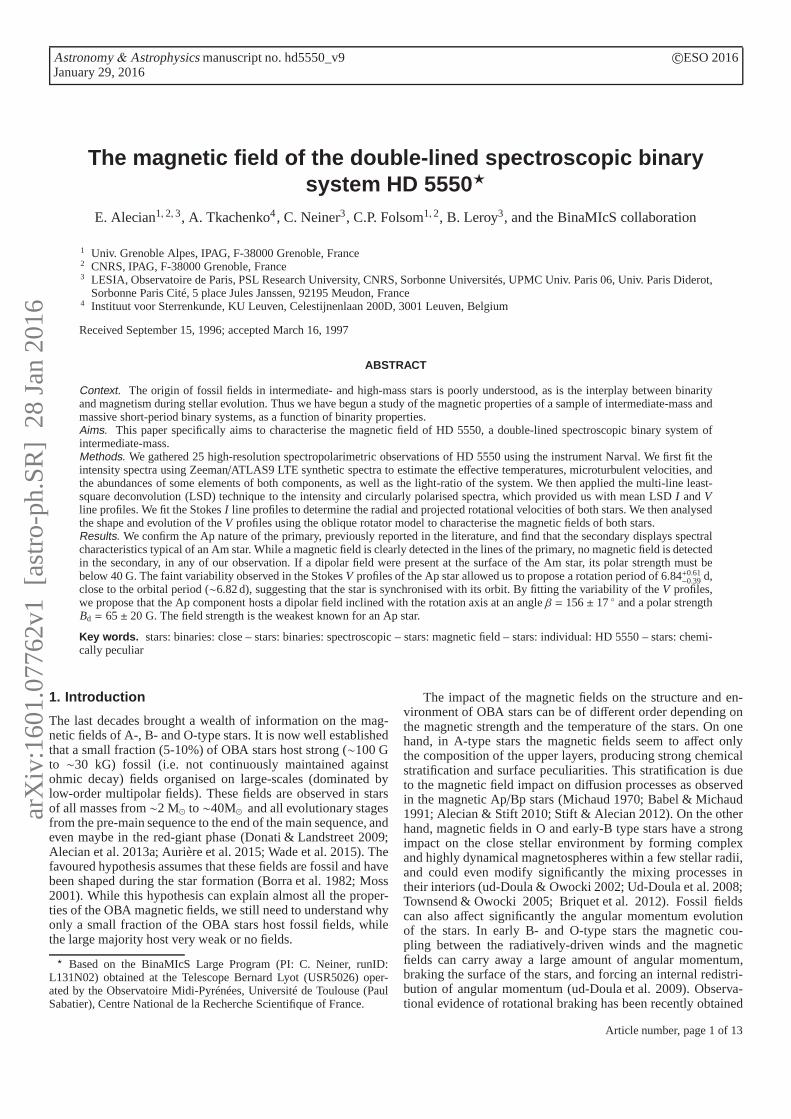
Fig. 3. Observation #1 (black solid line) superimposed with a Zeeman synthetic spectrum (dashed red line) computed with the parameters of Table3 and logg = 4.0. The main transition from the primary (P) or the secondary (S) are indicated with vertical blue bars.

spectra of the two stars, weighted by the square of the ratio ofradii.

The semi-automatic fitting procedure we have adopted con-sists in several steps. Assuming at first solar abundances, wehave alternatively fitted the parameters of one of the two com-ponents (Teff, vmic) and the ratio of radii (RA/RB) while fixingthe parameters of the other component, until a convergence wasfound (i.e. until a relative difference, between one iteration andthe next, below 3% was found for all the parameters). For bothstars, the rotational broadening and radial velocities were fixed tothe eye-fitting estimates. For each iteration, we have fittedsimul-taneously 17 spectral windows of 100 Å maximum width, dis-tributed between 4160 Å and 6460 Å, and avoiding the Balmerlines and the portions of the spectra heavily contaminated withtelluric lines. We then compared the result of the fit with theob-servation, and computed the localχ2 value for each spectral bin,as follows:

χ2i =

(

Ii obs− Ii mod

σ(Ii obs)

)2

(1)

This allows one to estimate the significance of the difference be-tween the observation and the model, and identify the elementswith the strongest anomalies. We found that the abundances ofsome elements (see Table 3) needed to be adjusted for both stars,in order to get a better agreement with the observations. To thisaim we proceeded as above by fitting the parameters of each star,alternatively, until a convergence was reached. For each star, wefit the abundances (logNX/NH) first, by fixing the fundamentalparameters (Teff, vmic, andRA/RB), and then fixed the abundancesto the new ones, and fit once more the fundamental parameters.We proceeded this way as many time as needed until conver-gence was reached. The whole procedure was applied one moretime using the more accurate values ofv sini, vrad andvth, derivedfrom the mean LSD profiles (Sect. 3.5).

3.2.3. Adopted parameters and uncertainty estimation

The uncertainties on the derived parameters can have manysources: uncertainties on logg, v sini, vth and spectral variability.Indeed, Ap stars often show rotational variability in theirspectradue to inhomogeneous abundance patches over the stellar sur-face or to rotational modulation of the Zeeman effect in individ-ual lines. We can therefore expect such variability in our spectra,which would imply uncertainties on the fundamental parametersobtained using only one observation at one rotation phase. Ad-ditional uncertainties could be caused by the blends of the pri-mary and secondary lines, which change with the orbital phase.To estimate the maximum effect on the fitted parameters, we se-lected two observations obtained at different orbital phases, androtational phases. The rotation period of the magnetic star, be-ing yet unknown, we based our choice on the amplitude of the

Zeeman signature of theV observations. We fixed our choiceto the spectra #1 and #11, and performed many semi-automaticfits by fixing the logg values to 4.0 and 4.5, and thev sini andvth to their minimum and maximum values given by their errorbars (Table 3). The average, minimum and maximum values ofall the solutions have been used to determine the adopted valuesand uncertainties on the effective temperatures, microturbulentvelocities, light-ratio, and abundances, summarised in Table 3.Our study confirms that the primary component is an Ap star,and we find that the secondary component is an Am star.

Table 3. Adopted fundamental parameters

Component A BRA/RB 1.24+0.04

−0.23

v sini (km s−1) 4.7+1.3−2.8 3.2+0.3

−1.9

vmic (km s−1) 0.0(8) 3.2+0.3−1.9

vth (km s−1) 1.9+1.5−1.9 4.0+1.3

−2.9

Teff (K) 11400(300) 7800+170−80

logg (cgs) [4.0,4.5]

logNX/NH

C -3.89(19)Mg -5.23(15)Ca -5.996(17)Sc -8.934(24)Ti -6.83(5)Cr -5.72(11) -5.96(6)Mn -6.28(18)Fe -4.36(11) -4.513(9)Ba -8.84(23)Pr -8.18(17)Nd -8.01(17)

Notes. The parameters that have been fitted in the fitting procedure arethose with the uncertainties indicated in brackets. The uncertainties re-fer to the last digits of the associated values. The parameters that havebeen fixed have no uncertainties. The two fixed values of logg used inthe procedure are indicated.

3.3. Extraction of the individual spectra

For the following magnetic analysis, we need to extract individ-ual spectra of both components separately for every observation.To this aim we first checked in the intensity spectra the variabil-ity of the lines of both components, and found that no strongvariability is affecting our data. We can therefore efficiently re-move the companion contamination from the combined spectrausing the disentangled ones, producing individual spectranor-malised to the summed continuum intensity of the binary. We fi-

Article number, page 5 of 13

A&A proofs:manuscript no. hd5550_v9

Fig. 4. Cr ii 5237 Å (left) and Feii 5427 Å (middle) lines of the primary, and Fei 4476 Å (right) line of the secondary, for the 19 observationsdescribed in the text (Sec. 3.3.1, overplotted coloured lines). The mean (diamonds) and standard deviations (verticalbars) of each pixel inside andaround the line have been overplotted and shifted by−0.05 in the y-direction for the left and right panels, and by−0.02 for the middle panelq.Red diamonds represent the pixels inside the spectral line,while blue diamonds represent the pixels in the local continuum. The averages of thestandard deviations inside the line (σ(line)) and in the continuum (σ(cont)) are indicated in the bottom left corners.

nally normalised the spectra to the correct continuum intensity ofthe considered star (primary or secondary) using the fundamen-tal parameters of Table 3. The whole procedure was first doneusing initial-estimate radial velocities, then done a second timeusing the radial velocities determined in Sec. 3.5. We describebelow the steps of the procedure.

3.3.1. Analysis of the variability of the spectra

We first selected the 19 observations at orbital phases wherethe radial velocities between both components are larger than30 km s−1. This allows us to study the variability inside the in-dividual spectral lines of each component without contamina-tion by spectral lines of the same transition from the companion.The temperature difference between both companions is largeenough to also create blends of lines of different transitions evenat large RV shifts, which is amplified by the abundance anoma-lies of both stars. We have therefore selected lines of the pri-mary and secondary that are not blended with any lines from thecompanion whatever the orbital phase. The number of the se-lected lines is less than 10 per component and they correspondto Cr, Fe and Mn for the primary, and Fe and Ti for the sec-ondary. For each line we proceeded as follows. We cancelledthe orbital RV shift and superimposed the lines of all 19 ob-servations. We finally measured the mean and standard devia-tion of each pixel inside the line, and compared them to the lo-cal continuum. An example of the overplotted spectral linesandthe mean and standard deviation for a few transitions is illus-trated in Fig. 4. In the secondary’s lines, the standard deviationsof the line pixels are of the same order as that of the contin-uum, indicating no significant variation of the spectral lines overthe 19 observations, while weak variability is observed in thelines of the primary. The expected main source of variability inAp stars is of rotational origin. According to the ratio of radii(RA/RB = 1.24+0.04

−0.23) and the large uncertainties on the ratio ofv sini (v siniA/v siniB= 1.5+3.1

−0.9), there is a possibility that thesystem could be synchronised (i.e.RA/RB =v siniA/v siniB). Wecannot therefore rule out the possibility that the orbital and rota-tion periods are identical. In that case, the variability ofthe linescannot be tested for RV differences below 30 km s−1.

3.3.2. Extraction and normalisation of the individual spectra

The individual spectra of both components have been extractedin the same way for all observations. We have shifted the dis-

entangled spectrum of the companion to the radial velocity ofthe companion for the relevant observation. We then subtractedthe shifted disentangled spectrum from the observation. Thisprovides the individual spectrum of the star normalised to thesummed continuum of the binary (IcA + IcB). To correct it fromthe continuum intensity of the companion, we computed theflux ratio as follows. The difference in temperatures between thecomponents is large enough for the flux ratio to be significantlydependent on wavelength. We used the fundamental parametersof Table 3 and the ZEEMAN code to compute the flux ratio overthe wavelength range of the disentangled spectra, as detailed inSect. 3.2.

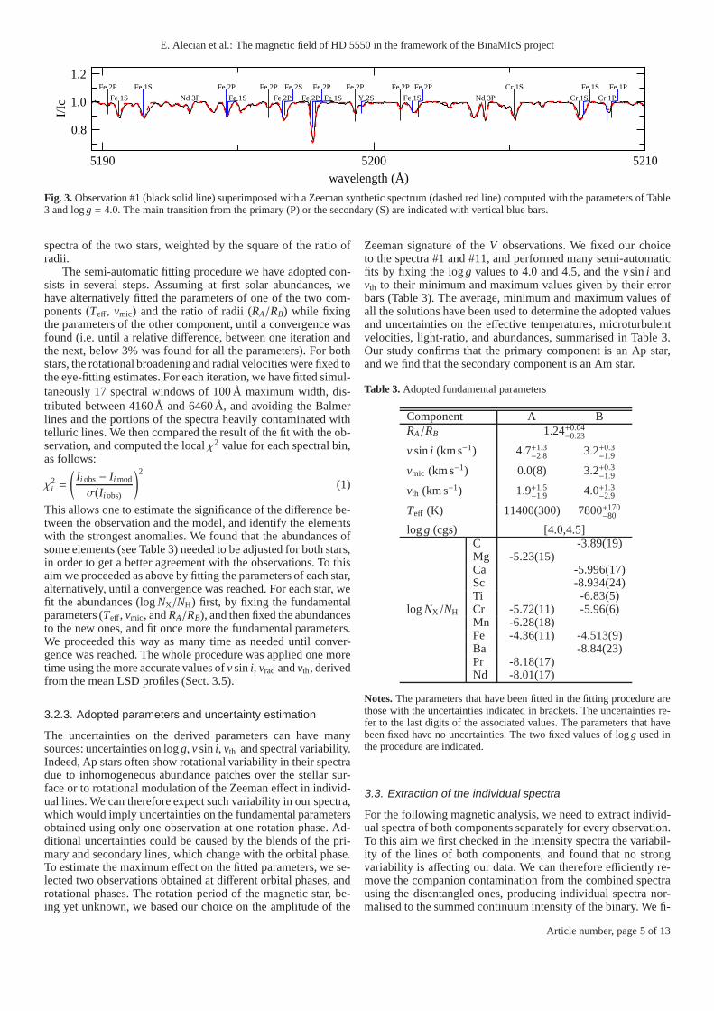
Fig. 5 illustrates a portion of the spectrum of the binary (theoriginal observation), and the extracted individual spectra of theprimary and secondary. The extracted spectra do not show anysignatures from the companion at the noise level. This is true forthe whole wavelength range and all the observations, indicatingthe success of the applied procedure.

3.4. Radial velocity determination

3.4.1. Least-squares deconvolution

We applied the Least Squares Deconvolution (LSD) procedureto our spectra (Donati et al. 1997). This procedure combinestheinformation contained in many metal lines of the spectrum, in or-der to extract the mean intensity (StokesI) and polarised (StokesV) line profiles. In StokesI, each line is weighted according toits central depth, while in StokesV the profiles are weightedaccording to the product of the central depth, wavelength andLandé factor. These parameters are contained in a ’line mask’derived from a synthetic spectrum corresponding to the effec-tive temperature and gravity of the star. The construction of theline mask for each star involved several steps. Our masks werefirst constructed using VALD line lists using stellar temperature,gravity, and abundances adapted to our stars. Our masks con-tain only lines with intrinsic depths larger or equal to 1% ofthecontinuum level. In a second step we excluded from the maskshydrogen Balmer lines, strong resonance lines, and lines con-taminated with telluric lines. Finally, we modified the intrinsicline depths in order to take into account the relative depth of thelines of the observed individual spectra. The last two stepsturnedout to be crucial for a reliable determination of the radial veloc-ities of both components, and therefore for ensuring the absenceof residuals from the companion in the individual spectra aftersubtracting the companion spectrum. Finally, the mean Landé

Article number, page 6 of 13

E. Alecian et al.: The magnetic field of HD 5550 in the framework of the BinaMIcS project

4500 4505 4510 4515 4520wavelength (Å)

0.2

0.4

0.6

0.8

1no

rmal

ised

inte

nsity

Fig. 5. Original combined (top, black) and re-normalised individual primary (middle, red) and secondary (bottom, blue) spectra of observation #1.The primary and secondary spectra have been shifted downward for display purpose.

factor, the mean wavelength, and the mean line depth used tonormalise theI andV profiles are respectively, 1.2, 500 nm, and0.2 of the continuum. The LSD S/N in V are given in column#2 of Table 4 for the primary mask, and in column #5 for thesecondary mask.

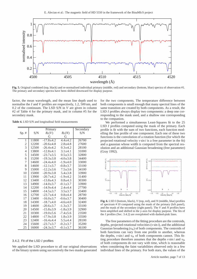
Table 4. LSD S/N and longitudinal field measurements

Primary SecondarySp. # S/N Bℓ(V) Bℓ(N) S/N

G G1 11800 -17.8±4.2 4.4±4.2 267002 12200 -20.6±4.8 2.8±4.8 276003 12500 -26.4±4.2 0.3±4.2 281004 13800 -12.8±4.1 3.1±4.1 310005 14500 -23.7±3.5 0.5±3.5 328006 15200 -19.3±3.8 -4.0±3.8 344007 14600 -24.4±4.0 -1.9±4.0 330008 14600 -12.1±3.7 -0.8±3.7 331009 15000 -12.2±3.6 7.5±3.6 34100

10 15000 -20.9±3.8 5.4±3.8 3390011 13900 -20.7±4.2 -1.9±4.2 3140012 13400 -13.8±4.3 0.8±4.3 3030013 14900 -14.0±3.7 -0.1±3.7 3390014 12200 -14.9±4.4 2.4±4.4 2770015 14800 -14.5±3.7 3.5±3.7 3340016 12700 -23.7±4.4 0.8±4.4 2870017 13400 -16.0±3.7 -0.6±3.7 3040018 14300 -18.7±4.0 -4.6±4.0 3240019 14600 -20.6±3.7 -1.3±3.7 3310020 14500 -15.8±3.9 -1.8±3.9 3290021 10300 -19.0±5.6 -7.4±5.6 2350022 14800 -17.9±3.8 1.8±3.9 3350023 12400 -16.4±4.4 5.5±4.4 2810024 15600 -23.7±3.7 -0.2±3.7 3520025 16000 -24.3±3.7 -0.1±3.7 36100

3.4.2. Fit of the LSD I profiles

We applied the LSD procedure to all our original observationsof the binary system using successively the two masks generated

for the two components. The temperature difference betweenboth components is small enough that many spectral lines of thesame transition are created by both components. As a result,theLSD I profiles always display two components: a deep one cor-responding to the mask used, and a shallow one correspondingto the companion.

We performed a simultaneous Least-Squares fit to the 25LSD I profiles computed using the mask of the primary. Eachprofile is fit with the sum of two functions, each function mod-elling the line profile of one component. Each one of these twofunctions is the convolution of a rotation function (for which theprojected rotational velocityv sini is a free parameter in the fit)and a gaussian whose width is computed from the spectral res-olution and an additional Gaussian broadening (free parameter)(Gray 1992).

Fig. 6. LSD I (bottom, black),V (top, red), andN (middle, blue) profilesof spectrum # 10 computed using the mask of the primary (left panel),and the mask of the secondary (right panel). TheV andN profiles havebeen amplified and shifted in the y-axis for display purpose.The fits ofthe I profiles (Sec. 3.4.2) are overplotted with dashed-pink lines.

The free parameters of the fitting procedure are the centroids,depths, projected rotational velocities (v sini), and the additionalGaussian broadening (vth) of both components. The centroids ofboth functions can vary from one profile to another, whereasthe depths,v sini andvth of both components cannot. This fit-ting procedure therefore assumes that the depthsv sini andvthof both components do not vary with time, which is reasonablewhen considering the faint variabilities observed only in afewindividual lines of the primary. For both stars, the values of the

Article number, page 7 of 13

A&A proofs:manuscript no. hd5550_v9

additional Gaussian broadening are found to be non-zero, andare required to fit well the wings of the lines. Thev sini of bothstars are indeed found to be relatively low (< 5 km s−1) and areclearly not dominating the broadening of the lines. As we haveremoved from the masks used to compute the LSD profiles allstrong lines for which the pressure or natural broadening aredominent, we interpret this additional Gaussian broadening asa local thermal Doppler broadening. Such broadening is faintenough to be usually ignored in case of fast rotation but cannotbe ignored in case of low rotation (v sini . 20 km s−1). Figure 6shows an example of such a fit for spectrum #10, for both masks.This automatic fitting procedure enables us to measure the radialvelocities with 1σ errors of 1.6− 1.8 km s−1for the primary (us-ing the primary mask), and 2− 3 km s−1for the secondary (usingthe secondary mask). Table 5 summarises our adopted radial ve-locity measurements for both components, while thev sini andvth are summarised in Table 3.

Table 5. Radial velocity measurements

Sp. # vradA vradB

km s−1 km s−1

1 10.6±1.8 -49.0±2.42 -30.4±1.8 14.2±3.23 -36.1±1.7 23.3±3.14 11.5±1.7 -50.6±3.05 -3.7±1.8 -27.2±3.16 -26.2±1.7 8.2±2.97 -36.9±1.8 26.1±3.18 -7.6±1.7 -20.2±2.49 9.9±1.8 -48.9±2.3

10 10.3±1.6 -47.4±2.311 -29.7±1.8 13.7±2.512 -37.3±1.8 25.0±2.413 -26.3±1.7 8.7±2.614 -3.6±1.8 -27.3±2.615 11.4±1.7 -50.8±2.416 -20.9±1.8 -0.4±2.317 12.6±1.7 -51.3±3.118 -33.3±1.8 19.2±2.419 7.6±1.7 -41.8±2.820 12.8±1.7 -50.7±2.121 -22.7±1.8 2.9±2.522 -31.4±1.7 17.3±2.623 7.9±1.7 -45.2±2.724 -5.2±1.7 -24.0±2.325 -26.1±1.7 8.3±2.5

4. Magnetic analysis of the primary star

4.1. The LSD V and N profiles

The LSDV profiles of our observations (see an example in Fig.6) show clear signatures in the primary component, but not inthesecondary. The false-alarm probabilities of the primary signa-tures, as defined by Donati et al. (1997), are all lower than 10−9

indicating that the signatures are all significant (definitedetec-tions). The signatures display a typical Zeeman S-shape. Theyare centred on the centroid of the primary component, and areasbroad as the primaryI profiles. TheN profiles display flat signalin all our observations indicating that theV profiles are not con-taminated with spurious signal. All of which allows us to confi-dently conclude that a magnetic field is detected at the surface of

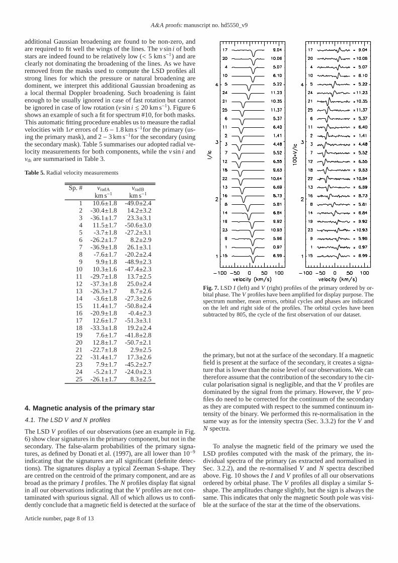
Fig. 7. LSD I (left) andV (right) profiles of the primary ordered by or-bital phase. TheV profiles have been amplified for display purpose. Thespectrum number, mean errors, orbital cycles and phases areindicatedon the left and right side of the profiles. The orbital cycles have beensubtracted by 805, the cycle of the first observation of our dataset.

the primary, but not at the surface of the secondary. If a magneticfield is present at the surface of the secondary, it creates a signa-ture that is lower than the noise level of our observations. We cantherefore assume that the contribution of the secondary to the cir-cular polarisation signal is negligible, and that theV profiles aredominated by the signal from the primary. However, theV pro-files do need to be corrected for the continuum of the secondaryas they are computed with respect to the summed continuum in-tensity of the binary. We performed this re-normalisation in thesame way as for the intensity spectra (Sec. 3.3.2) for theV andN spectra.

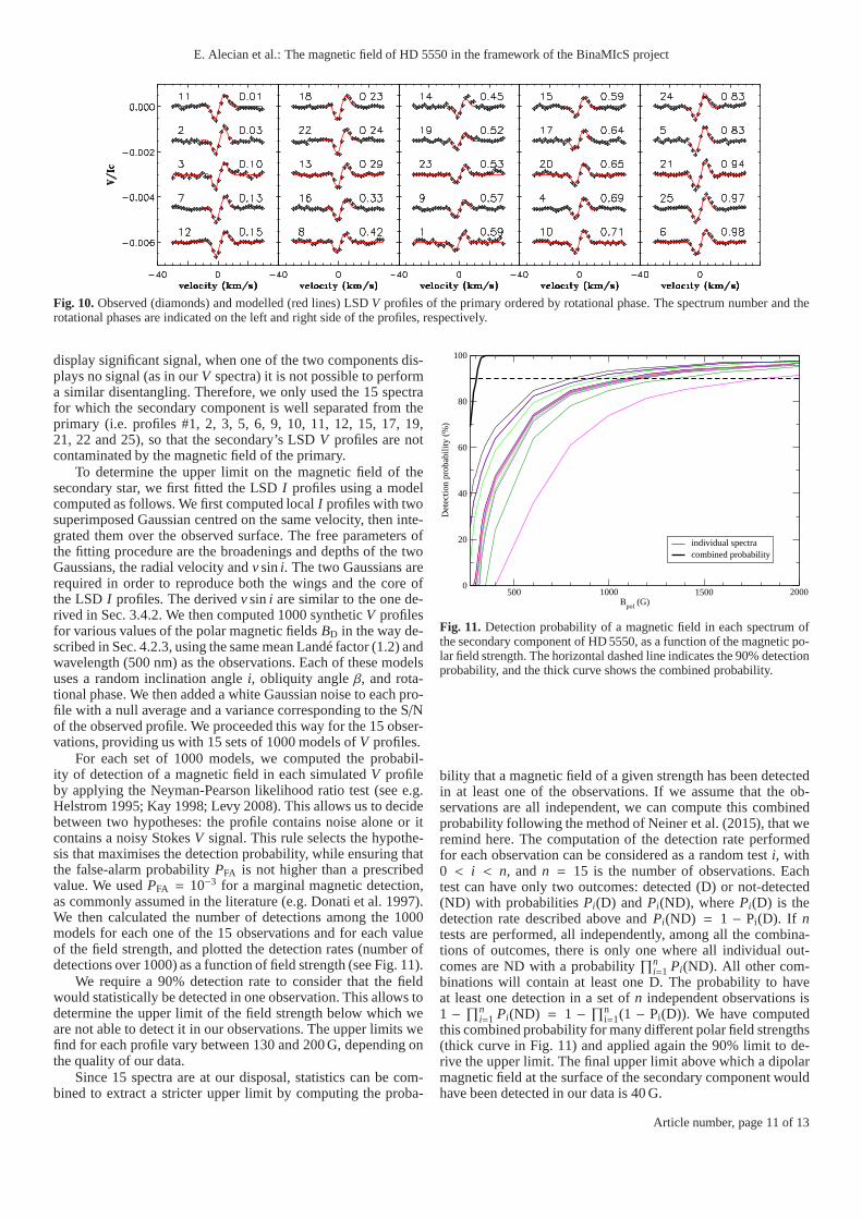
To analyse the magnetic field of the primary we used theLSD profiles computed with the mask of the primary, the in-dividual spectra of the primary (as extracted and normalised inSec. 3.2.2), and the re-normalisedV and N spectra describedabove. Fig. 10 shows theI andV profiles of all our observationsordered by orbital phase. TheV profiles all display a similar S-shape. The amplitudes change slightly, but the sign is always thesame. This indicates that only the magnetic South pole was visi-ble at the surface of the star at the time of the observations.

Article number, page 8 of 13

E. Alecian et al.: The magnetic field of HD 5550 in the framework of the BinaMIcS project

4.2. Determination of the rotation period

The magnetic fields of Ap stars are in most cases dominated bya strong dipolar component. In a few cases a quadrupolar or oc-tupolar component can be as large or even larger than the dipolarone, but in any case the dominant component is a low-order mul-tipolar field. The magnetic axes are usually inclined with respectto the rotation axis, causing rotational modulation of the longi-tudinal magnetic field at the surface. We can therefore expectperiodic variability in our data directly linked to the rotation pe-riod at the surface of the star. We can use this variability oftheV profiles to find the rotation period. To this aim we applied var-ious methods described below.

4.2.1. Search for the rotation period using the longitudinalfield measurements

We measured the line-of-sight component of the magnetic fieldintegrated over the stellar surface (the longitudinal fieldBℓ) fromour data by computing the first order moment ofV and theequivalent width ofI using the method described by Wade et al.(2000). We used integration limits of 23 km s−1 wide centred onthe radial velocity of theI profiles. The values we find are allnegative, and range from∼−26 G to∼−12 G, with typical er-ror bars of about 4 G. Using the same method, we measured thelongitudinal field values in the LSDN profiles. All values arefound to be consistent with 0 G, confirming the absence of spu-rious polarisation in our data. TheBℓ measurements forV andthe pseudo-Bℓ measurements forN are given in columns #3 and#4 of Table 4.

We searched for periodic variations in theBl values usingtwo methods: a simple sine fit to theBl values, and a cleanmethod. The software we used for these searches are describedin Gutiérrez-Soto et al. (2009). The sine fit provided two signifi-cant periods at 5.80 and 6.82 d. The clean method provided peaksaround 5.68, 6.45, 2.63, 3.55 d. None of these periods are iden-tical, we conclude that no periodicity can be found in theBl val-ues. However, we note that one of the periods we found (6.82 d)is close to the orbital period.

4.2.2. Search for the rotation period using the Stokes Vprofiles

Finally, we attempted a search for periodicity using the entireV profiles, using both model-independent and model-dependentmethods.

Model-independent methodsWe first performed a frequency analysis using various meth-

ods. We first used the FAMIAS package4 (Zima 2008). Using amean 1D Fourier technique applied to the LSD StokesV pro-files and a S/N significance criterion of 4, we obtained a mainfrequency peak atf1 =1.14533 c.d−1 with S/N=18, and its 1-daliases at∼0.14, 2.14, 3.14, etc. We also detect peaks at 1, 2, 3,...c.d−1 and combinations of these peaks withf1 at 0.856 c.d−1,etc. Then, we applied the mean 1D Fourier method of FAMIASto the LSD I profiles. We found a frequency at 0.14745 c.d−1

with S/N=9. Again we also find 1-d aliases and combinations.From this frequency analysis of theV andI profiles, we conclude

4 The software package FAMIAS was developed in the frame-work of the FP6 European Coordination Action HELAS(http://www.helas-eu.org/)

that f ∼[0.145-0.148] c.d−1 is the main frequency of variationsof HD 5550, corresponding to a period comprised between 6.75and 6.90 d.

We then fit the individual variation of each pixel within theVprofiles (within±10 km s−1of the line center) with a sinusoidalfunction with three free parameters (amplitude, zero pointandphase) with a fixed period. This was done for each pixel, formany periods between between 0.3 and 50 days, constructing aperiodogram inχ2 and period for that pixel. We then computedthe average of all the periodograms, and looked for mimima inχ2

(Fig. 8). Only one significant minimum at a 5-σ confidence levelis found above 1.2 d, at a period of 6.84± 0.15 d with a reducedχ2 of 0.62. Below 1.2 d there are significant aliasing. However,those periods are highly improbable with the observedv sini,and the magnetic and binary nature of the target. Furthermore,the temporal sampling of our observations suggests we do nothave much sensitivity below 1.2 d.

0 10 20 30 40 50Period (days)

0

1

2

3

4

χ ν2

Fig. 8. Periodogram of the LSDV profiles of the magnetic Ap compo-nent.

Model-dependent methodThe last method we employed has already been described

in detail in Alecian et al. (2008). We assume that the magneticfield of the primary component is a dipole, centered inside thestar, and inclined to the rotation axis by an obliquity angleβ.The rotation axis is inclined with respect to the line-of-sight byan anglei, and the magnetic strength at the pole is defined asBD(Fig. 9). The magnetic pole points towards the observer at phase0.0 (given by the initial epochT0). If both positive and negativepoles are observed over one rotation cycle, then we choose thepositive magnetic pole to point towards the observer at phase0.0. We compute the local intensity line profiles on each point ofa 5041 elements grid simulating the observed surface of the star.The localI profile is a Gaussian with a width dependent on theinstrumental and local thermal broadening, shifted to the localradial velocity according to the givenv sini. The localV profilesare computed in the weak field approximation using the localI profiles, a mean wavelength of 500 nm, and a mean Landéfactor of 1.2, equal to the normalised values used in the LSDcomputation. TheV and I profiles are then integrated over thesurface using a linear limb-darkening law with a coefficient of0.43, suitable for the temperature of the star (Claret & Bloemen2011), and for given values of the rotation phase (φ), i, β andBD.The rotation phase is obtained from the rotation period (Prot),

Article number, page 9 of 13

A&A proofs:manuscript no. hd5550_v9

Fig. 9. A 3D schematic view of the magnetic star at the rotation phase0.0 of our modeling (see the text). The rotation (red, labelledΩ), mag-netic (blue, labelledB), and cartesian (x,y,z) axes are represented out-side (full lines) and inside the star (dotted lines). Thex axis is pointingtowards the observer. The arrows representing the inclination angle (i)and magnetic obliquity (β) angles point towards positive values. Theparallels at 30, 60 and 90 of latitude are plotted with respect to the ro-tation axis for display purpose. The arrows superimposed with the par-allels indicate the direction of rotation of the star. The positive magneticpole (⊕) is plotted as a large blue dot at the intersection of the magneticaxis and the surface of the star.

T0, and the HJD of our observations. For all our observations,we computed a grid of StokesV profiles for various values ofProt (between 1 and 66 d),φ0 (the phase shift betweenT0 andthe HJD of our first observation, varying from 0 to 1),i (between0 and 180), β (between 0 and 180), andBD (between 20 and1000 G). We then computed theχ2 on each point of the grid.Next, we searched for the minimum ofχ2 as a function of therotation period. We find a periodogram very similar to Fig. 8,with only one significant minimum at 6.84 d, with a reducedχ2

of 1.3, and aliasing below 1.2 d.

4.2.3. Conclusions from the rotation period search

We used many different methods to attempt to find a period inourV profiles, as well as in ourI profiles (assuming that the faintvariabilities observed in theI profiles are of rotational origin).We found no common period to all the methods. On the otherhand, all the methods we employed using the entire StokesVprofiles provide us with a common period at 6.84 d. Assumingthis period, the evolution of the profiles as a function of phaseappears coherent with a simple dipolar field for all the profiles.

We estimate the uncertainties of the rotation period at a 3σconfidence level to be 6.84+0.61

−0.39d. This indicates that the rotationperiod is similar to the orbital one (Porb = 6.82054d), whichwould imply that the system is synchronised. We have alreadyreported above that our measurements of thev sini and the ra-tio of radii permits the system to be synchronised. Furthermore,the system is almost circularised (e = 0.005), and the evolution-ary models of a binary system predict that the synchronisationtime is shorter than the circularisation time (Zahn 1977). It is

therefore very likely that HD 5550 is already synchronised,sup-porting our rotation period determination.

4.3. The magnetic topology of the primary

We assume a rotation period of 6.84 d, and propose a solution forthe magnetic topology of the primary. The oblique rotator modelused to fit theV profiles has already been described in Sect.4.2.3. The best model corresponds toi = 32+21

−38, β = 156±17,

andBd = 65±20 G, where the error bars correspond to a 3σ con-fidence level, based onχ2 statistics. The rotational initial epochis found to beT0 = 2 456 481.5± 0.8, which corresponds to aphase shift from the orbital initial epoch of about 0.6. In orderto check the uniqueness of the solution we plottedχ2 maps asa function of two of the four fitted parameters (T0, i, β, BD), byfixing the other parameters to the values at minimum. We plotteda total of 6 maps corresponding to all possible combinationsof2 parameters among 4, and found no otherχ2 minimum. TheVprofiles corresponding to this solution are plotted over theob-servations in Fig. 10. We find that the model reproduces wellthe observations. The uncertainties on the parameters are ratherlarge, which is a consequence on the faint variability of theVprofiles over the rotation cycle.

The uncertainty on the flux ratio between both componentscomputed in Sec. 3.3 has not been taken into account in theabove study. The uncertainty on the flux ratio is controlled bythe uncertainty on the radii ratio (RA/RB) and on the tempera-tures ratio (TeffA/TeffB). The former is the dominant uncertainty,and does not depend on wavelength, while the later is well con-strained, but is dependent on the wavelength. As bothI andVprofiles are computed with respect to the continuum, the uncer-tainty on the radii ratio has no impact on the magnetic model wederived (the continuum terms effectively cancel out). However,the wavelength dependency of the temperature ratio can affectthe solutions of the LSD calculations. To estimate the impact ofthe uncertainty of the temperature ratio on our solution we havecomputedI andV LSD profiles of the primary without correct-ing the continuum for the secondary’s contribution, simulating avery extreme case with a temperature ratio of 1. We find a so-lution very similar to the above solution, and consistent withinthe error bars. We can therefore neglect the uncertainty on thetemperature ratio in our final solution.

5. Upper limit on the magnetic field of thesecondary star

As detailed above, we do not detect a magnetic field at the sur-face of the secondary component of HD 5550 in our data. Thelongitudinal field values we measured by integrating the LSDIandV profiles around±12 km s−1of the line center, are all consis-tent with zero with uncertainties comprised between 3 and 4 G.

The signature of a weak magnetic field may have remainedhidden in the noise of the spectra of the secondary component.We propose to estimate its maximum strength assuming the sim-plest magnetic configuration, i.e. a dipole. To this aim, we needto isolate LSDI and V profiles of the secondary without anycontamination from the primary for as many observations aspossible. Unfortunately, as described above, the LSD profiles,computed with the line-mask tailored for the secondary, arecon-taminated by the primary. This is problematic near conjunctionwhen both line components are partially or entirely superim-posed. While it is possible to disentangle the signals of bothcomponents in the intensity spectrum because both components

Article number, page 10 of 13

E. Alecian et al.: The magnetic field of HD 5550 in the framework of the BinaMIcS project

Fig. 10. Observed (diamonds) and modelled (red lines) LSDV profiles of the primary ordered by rotational phase. The spectrum number and therotational phases are indicated on the left and right side ofthe profiles, respectively.

display significant signal, when one of the two components dis-plays no signal (as in ourV spectra) it is not possible to performa similar disentangling. Therefore, we only used the 15 spectrafor which the secondary component is well separated from theprimary (i.e. profiles #1, 2, 3, 5, 6, 9, 10, 11, 12, 15, 17, 19,21, 22 and 25), so that the secondary’s LSDV profiles are notcontaminated by the magnetic field of the primary.

To determine the upper limit on the magnetic field of thesecondary star, we first fitted the LSDI profiles using a modelcomputed as follows. We first computed localI profiles with twosuperimposed Gaussian centred on the same velocity, then inte-grated them over the observed surface. The free parameters ofthe fitting procedure are the broadenings and depths of the twoGaussians, the radial velocity andv sini. The two Gaussians arerequired in order to reproduce both the wings and the core ofthe LSDI profiles. The derivedv sini are similar to the one de-rived in Sec. 3.4.2. We then computed 1000 syntheticV profilesfor various values of the polar magnetic fieldsBD in the way de-scribed in Sec. 4.2.3, using the same mean Landé factor (1.2)andwavelength (500 nm) as the observations. Each of these modelsuses a random inclination anglei, obliquity angleβ, and rota-tional phase. We then added a white Gaussian noise to each pro-file with a null average and a variance corresponding to the S/Nof the observed profile. We proceeded this way for the 15 obser-vations, providing us with 15 sets of 1000 models ofV profiles.

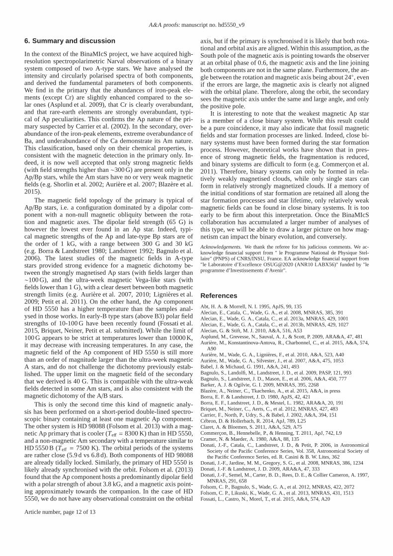
For each set of 1000 models, we computed the probabil-ity of detection of a magnetic field in each simulatedV profileby applying the Neyman-Pearson likelihood ratio test (see e.g.Helstrom 1995; Kay 1998; Levy 2008). This allows us to decidebetween two hypotheses: the profile contains noise alone or itcontains a noisy StokesV signal. This rule selects the hypothe-sis that maximises the detection probability, while ensuring thatthe false-alarm probabilityPFA is not higher than a prescribedvalue. We usedPFA = 10−3 for a marginal magnetic detection,as commonly assumed in the literature (e.g. Donati et al. 1997).We then calculated the number of detections among the 1000models for each one of the 15 observations and for each valueof the field strength, and plotted the detection rates (number ofdetections over 1000) as a function of field strength (see Fig. 11).

We require a 90% detection rate to consider that the fieldwould statistically be detected in one observation. This allows todetermine the upper limit of the field strength below which weare not able to detect it in our observations. The upper limits wefind for each profile vary between 130 and 200 G, depending onthe quality of our data.

Since 15 spectra are at our disposal, statistics can be com-bined to extract a stricter upper limit by computing the proba-

500 1000 1500 2000B

pol (G)

0

20

40

60

80

100

Det

ectio

n pr

obab

ility

(%

)

individual spectracombined probability

Fig. 11. Detection probability of a magnetic field in each spectrum ofthe secondary component of HD 5550, as a function of the magnetic po-lar field strength. The horizontal dashed line indicates the90% detectionprobability, and the thick curve shows the combined probability.

bility that a magnetic field of a given strength has been detectedin at least one of the observations. If we assume that the ob-servations are all independent, we can compute this combinedprobability following the method of Neiner et al. (2015), that weremind here. The computation of the detection rate performedfor each observation can be considered as a random testi, with0 < i < n, andn = 15 is the number of observations. Eachtest can have only two outcomes: detected (D) or not-detected(ND) with probabilitiesPi(D) and Pi(ND), wherePi(D) is thedetection rate described above andPi(ND) = 1 − Pi(D). If ntests are performed, all independently, among all the combina-tions of outcomes, there is only one where all individual out-comes are ND with a probability

∏ni=1 Pi(ND). All other com-

binations will contain at least one D. The probability to haveat least one detection in a set ofn independent observations is1 −

∏ni=1 Pi(ND) = 1 −

∏ni=1(1 − Pi(D)). We have computed

this combined probability for many different polar field strengths(thick curve in Fig. 11) and applied again the 90% limit to de-rive the upper limit. The final upper limit above which a dipolarmagnetic field at the surface of the secondary component wouldhave been detected in our data is 40 G.

Article number, page 11 of 13

A&A proofs:manuscript no. hd5550_v9

6. Summary and discussion

In the context of the BinaMIcS project, we have acquired high-resolution spectropolarimetric Narval observations of a binarysystem composed of two A-type stars. We have analysed theintensity and circularly polarised spectra of both components,and derived the fundamental parameters of both components.We find in the primary that the abundances of iron-peak ele-ments (except Cr) are slightly enhanced compared to the so-lar ones (Asplund et al. 2009), that Cr is clearly overabundant,and that rare-earth elements are strongly overabundant, typi-cal of Ap peculiarities. This confirms the Ap nature of the pri-mary suspected by Carrier et al. (2002). In the secondary, over-abundance of the iron-peak elements, extreme overabundance ofBa, and underabundance of the Ca demonstrate its Am nature.This classification, based only on their chemical properties, isconsistent with the magnetic detection in the primary only.In-deed, it is now well accepted that only strong magnetic fields(with field strengths higher than∼300 G) are present only in theAp/Bp stars, while the Am stars have no or very weak magneticfields (e.g. Shorlin et al. 2002; Aurière et al. 2007; Blazèreet al.2015).

The magnetic field topology of the primary is typical ofAp/Bp stars, i.e. a configuration dominated by a dipolar com-ponent with a non-null magnetic obliquity between the rota-tion and magnetic axes. The dipolar field strength (65 G) ishowever the lowest ever found in an Ap star. Indeed, typi-cal magnetic strengths of the Ap and late-type Bp stars are ofthe order of 1 kG, with a range between 300 G and 30 kG(e.g. Borra & Landstreet 1980; Landstreet 1992; Bagnulo et al.2006). The latest studies of the magnetic fields in A-typestars provided strong evidence for a magnetic dichotomy be-tween the strongly magnetised Ap stars (with fields larger than∼100 G), and the ultra-week magnetic Vega-like stars (withfields lower than 1 G), with a clear desert between both magneticstrength limits (e.g. Aurière et al. 2007, 2010; Lignières et al.2009; Petit et al. 2011). On the other hand, the Ap componentof HD 5550 has a higher temperature than the samples anal-ysed in those works. In early-B type stars (above B3) polar fieldstrengths of 10-100 G have been recently found (Fossati et al.2015, Briquet, Neiner, Petit et al. submitted). While the limit of100 G appears to be strict at temperatures lower than 10000K,it may decrease with increasing temperatures. In any case, themagnetic field of the Ap component of HD 5550 is still morethan an order of magnitude larger than the ultra-week magneticA stars, and do not challenge the dichotomy previously estab-lished. The upper limit on the magnetic field of the secondarythat we derived is 40 G. This is compatible with the ultra-weakfields detected in some Am stars, and is also consistent with themagnetic dichotomy of the A/B stars.

This is only the second time this kind of magnetic analy-sis has been performed on a short-period double-lined spectro-scopic binary containing at least one magnetic Ap component.The other system is HD 98088 (Folsom et al. 2013) with a mag-netic Ap primary that is cooler (Teff = 8300 K) than in HD 5550,and a non-magnetic Am secondary with a temperature similar toHD 5550 B (Teff = 7500 K). The orbital periods of the systemsare rather close (5.9 d vs 6.8 d). Both components of HD 98088are already tidally locked. Similarly, the primary of HD 5550 islikely already synchronised with the orbit. Folsom et al. (2013)found that the Ap component hosts a predominantly dipolar fieldwith a polar strength of about 3.8 kG, and a magnetic axis point-ing approximately towards the companion. In the case of HD5550, we do not have any observational constraint on the orbital

axis, but if the primary is synchronised it is likely that both rota-tional and orbital axis are aligned. Within this assumption, as theSouth pole of the magnetic axis is pointing towards the observerat an orbital phase of 0.6, the magnetic axis and the line joiningboth components are not in the same plane. Furthermore, the an-gle between the rotation and magnetic axis being about 24, evenif the errors are large, the magnetic axis is clearly not alignedwith the orbital plane. Therefore, along the orbit, the secondarysees the magnetic axis under the same and large angle, and onlythe positive pole.

It is interesting to note that the weakest magnetic Ap staris a member of a close binary system. While this result couldbe a pure coincidence, it may also indicate that fossil magneticfields and star formation processes are linked. Indeed, close bi-nary systems must have been formed during the star formationprocess. However, theoretical works have shown that in pres-ence of strong magnetic fields, the fragmentation is reduced,and binary systems are difficult to form (e.g. Commerçon et al.2011). Therefore, binary systems can only be formed in rela-tively weakly magnetised clouds, while only single stars canform in relatively strongly magnetized clouds. If a memory ofthe initial conditions of star formation are retained all along thestar formation processes and star lifetime, only relatively weakmagnetic fields can be found in close binary systems. It is tooearly to be firm about this interpretation. Once the BinaMIcScollaboration has accumulated a larger number of analyses ofthis type, we will be able to draw a larger picture on how mag-netism can impact the binary evolution, and conversely.

Acknowledgements. We thank the referee for his judicious comments. We ac-knowledge financial support from " le Programme National de Physique Stel-laire" (PNPS) of CNRS/INSU, France. EA acknowledge financial support from"le Laboratoire d’Excellence OSUG@2020 (ANR10 LABX56)" funded by "leprogramme d’Investissements d’Avenir".

References

Abt, H. A. & Morrell, N. I. 1995, ApJS, 99, 135Alecian, E., Catala, C., Wade, G. A., et al. 2008, MNRAS, 385,391Alecian, E., Wade, G. A., Catala, C., et al. 2013a, MNRAS, 429, 1001Alecian, E., Wade, G. A., Catala, C., et al. 2013b, MNRAS, 429, 1027Alecian, G. & Stift, M. J. 2010, A&A, 516, A53Asplund, M., Grevesse, N., Sauval, A. J., & Scott, P. 2009, ARA&A, 47, 481Aurière, M., Konstantinova-Antova, R., Charbonnel, C., etal. 2015, A&A, 574,

A90Aurière, M., Wade, G. A., Lignières, F., et al. 2010, A&A, 523, A40Aurière, M., Wade, G. A., Silvester, J., et al. 2007, A&A, 475, 1053Babel, J. & Michaud, G. 1991, A&A, 241, 493Bagnulo, S., Landolfi, M., Landstreet, J. D., et al. 2009, PASP, 121, 993Bagnulo, S., Landstreet, J. D., Mason, E., et al. 2006, A&A, 450, 777Barker, A. J. & Ogilvie, G. I. 2009, MNRAS, 395, 2268Blazère, A., Neiner, C., Tkachenko, A., et al. 2015, A&A, in pressBorra, E. F. & Landstreet, J. D. 1980, ApJS, 42, 421Borra, E. F., Landstreet, J. D., & Mestel, L. 1982, ARA&A, 20,191Briquet, M., Neiner, C., Aerts, C., et al. 2012, MNRAS, 427, 483Carrier, F., North, P., Udry, S., & Babel, J. 2002, A&A, 394, 151Cébron, D. & Hollerbach, R. 2014, ApJ, 789, L25Claret, A. & Bloemen, S. 2011, A&A, 529, A75Commerçon, B., Hennebelle, P., & Henning, T. 2011, ApJ, 742,L9Cramer, N. & Maeder, A. 1980, A&A, 88, 135Donati, J.-F., Catala, C., Landstreet, J. D., & Petit, P. 2006, in Astronomical

Society of the Pacific Conference Series, Vol. 358, Astronomical Society ofthe Pacific Conference Series, ed. R. Casini & B. W. Lites, 362

Donati, J.-F., Jardine, M. M., Gregory, S. G., et al. 2008, MNRAS, 386, 1234Donati, J.-F. & Landstreet, J. D. 2009, ARA&A, 47, 333Donati, J.-F., Semel, M., Carter, B. D., Rees, D. E., & Collier Cameron, A. 1997,

MNRAS, 291, 658Folsom, C. P., Bagnulo, S., Wade, G. A., et al. 2012, MNRAS, 422, 2072Folsom, C. P., Likuski, K., Wade, G. A., et al. 2013, MNRAS, 431, 1513Fossati, L., Castro, N., Morel, T., et al. 2015, A&A, 574, A20

Article number, page 12 of 13

E. Alecian et al.: The magnetic field of HD 5550 in the framework of the BinaMIcS project

Gray, D. F. 1992, The observation and analysis of stellar photospheres (Cam-bridge Astrophysics Series, Cambridge: Cambridge University Press, 1992,2nd ed., ISBN 0521403200.)

Gregory, S. G., Holzwarth, V. R., Donati, J.-F., et al. 2014,in European Physi-cal Journal Web of Conferences, Vol. 64, European Physical Journal Web ofConferences, 8009

Gutiérrez-Soto, J., Floquet, M., Samadi, R., et al. 2009, A&A, 506, 133Hadrava, P. 1995, A&AS, 114, 393Helstrom, C. W. 1995, Elements of Signal Detection and Estimation (Prentice

Hall)Hut, P. 1980, A&A, 92, 167Ilijic, S., Hensberge, H., Pavlovski, K., & Freyhammer, L. M. 2004, in Astro-

nomical Society of the Pacific Conference Series, Vol. 318, Spectroscopicallyand Spatially Resolving the Components of the Close Binary Stars, ed. R. W.Hilditch, H. Hensberge, & K. Pavlovski, 111–113

Kay, S. M. 1998, Fundamentals of Statistical Signal Processing, Volume 2: De-tection Theory (Prentice Hall)

Landstreet, J. D. 1988, ApJ, 326, 967Landstreet, J. D. 1992, A&A Rev., 4, 35Levy, B. C. 2008, Principles of Signal Detection and Parameter Estimation

(Springer)Lignières, F., Petit, P., Böhm, T., & Aurière, M. 2009, A&A, 500, L41Masson, J., Teyssier, R., Mulet-Marquis, C., Hennebelle, P., & Chabrier, G.

2012, ApJS, 201, 24Michaud, G. 1970, ApJ, 160, 641Moss, D. 2001, in Astronomical Society of the Pacific Conference Series,

Vol. 248, Magnetic Fields Across the Hertzsprung-Russell Diagram, ed.G. Mathys, S. K. Solanki, & D. T. Wickramasinghe, 305

Neiner, C., Grunhut, J., Leroy, B., De Becker, M., & Rauw, G. 2015, A&A, 575,A66

North, P. & Cramer, N. 1984, A&AS, 58, 387Ogilvie, G. I. & Lin, D. N. C. 2007, ApJ, 661, 1180Petit, P., Lignières, F., Aurière, M., et al. 2011, A&A, 532,L13Remus, F., Mathis, S., & Zahn, J.-P. 2012, A&A, 544, A132Renson, P., Gerbaldi, M., & Catalano, F. A. 1991, A&AS, 89, 429Russell, C. M. P., Corcoran, M. F., Okazaki, A. T., Madura, T.I., & Owocki, S. P.

2011, Bulletin de la Societe Royale des Sciences de Liege, 80, 719Shorlin, S. L. S., Wade, G. A., Donati, J.-F., et al. 2002, A&A, 392, 637Silvester, J., Wade, G. A., Kochukhov, O., et al. 2012, MNRAS, 426, 1003Simon, K. P. & Sturm, E. 1994, A&A, 281, 286Stepien, K. 2000, A&A, 353, 227Stift, M. J. & Alecian, G. 2012, MNRAS, 425, 2715Townsend, R. H. D., Oksala, M. E., Cohen, D. H., Owocki, S. P.,& ud-Doula,

A. 2010, ApJ, 714, L318Townsend, R. H. D. & Owocki, S. P. 2005, MNRAS, 357, 251ud-Doula, A., Owocki, S., Townsend, R., Petit, V., & Cohen, D. 2014, MNRAS,

441, 3600ud-Doula, A. & Owocki, S. P. 2002, ApJ, 576, 413Ud-Doula, A., Owocki, S. P., & Townsend, R. H. D. 2008, MNRAS,385, 97ud-Doula, A., Owocki, S. P., & Townsend, R. H. D. 2009, MNRAS,392, 1022Wade, G. A., Bagnulo, S., Kochukhov, O., et al. 2001, A&A, 374, 265Wade, G. A., Donati, J.-F., Landstreet, J. D., & Shorlin, S. L. S. 2000, MNRAS,

313, 823Wade, G. A., Neiner, C., Alecian, E., et al. 2015, in MNRAS, submittedZahn, J.-P. 1977, A&A, 57, 383Zima, W. 2008, Communications in Asteroseismology, 155, 17

Article number, page 13 of 13