Efficient Circuit-based PSI via Cuckoo Hashing (Full Version) ? Benny Pinkas 1 , Thomas Schneider 2 , Christian Weinert 2 , and Udi Wieder 3 1 Bar-Ilan University [email protected]2 TU Darmstadt {thomas.schneider,christian.weinert}@crisp-da.de 3 VMware Research [email protected]Abstract. While there has been a lot of progress in designing efficient custom protocols for computing Private Set Intersection (PSI), there has been less research on using generic Multi-Party Computation (MPC) protocols for this task. However, there are many variants of the set intersection functionality that are not addressed by the existing custom PSI solutions and are easy to compute with generic MPC protocols (e.g., comparing the cardinality of the intersection with a threshold or measuring ad conversion rates). Generic PSI protocols work over circuits that compute the intersection. For sets of size n, the best known circuit constructions conduct O(n log n) or O(n log n/ log log n) comparisons (Huang et al., NDSS’12 and Pinkas et al., USENIX Security’15). In this work, we propose new circuit-based protocols for computing variants of the intersection with an almost linear number of comparisons. Our constructions are based on new variants of Cuckoo hashing in two dimensions. We present an asymptotically efficient protocol as well as a protocol with better concrete efficiency. For the latter protocol, we determine the required sizes of tables and circuits experimentally, and show that the run-time is concretely better than that of existing constructions. The protocol can be extended to a larger number of parties. The proof technique for analyzing Cuckoo hashing in two dimensions is new and can be generalized to analyzing standard Cuckoo hashing as well as other new variants of it. Keywords: Private Set Intersection, Secure Computation 1 Introduction Private Set Intersection (PSI) refers to a protocol which enables two parties, holding respective input sets X and Y , to compute the intersection X ∩ Y without revealing any information about the items which are not in the intersection. The PSI functionality is useful for applications where parties need to apply a JOIN operation to private datasets. There are multiple constructions of secure protocols for computing PSI, but there is an advantage for computing PSI by applying a generic Multi-Party Computation (MPC) protocol to a circuit computing the intersection (see §1.1). The problem is that a naive circuit computes O(n 2 ) comparisons, and even the most recent circuit-based constructions require O(n log n) or O(n log n/ log log n) comparisons (see §1.4). In this work, we present a new circuit-based protocol for computing PSI variants. In our protocol, each party first inserts its input elements into bins according to a new hashing algorithm, and then the intersection is computed by securely computing a Boolean comparison circuit over the bins. The insertion of the items is based on new Cuckoo hashing variants which guarantee that if the two ? Please cite the conference version of this work published at EUROCRYPT’18 [PSWW18].
Transcript
Efficient Circuit-based PSI via Cuckoo Hashing
(Full Version)?
Benny Pinkas1, Thomas Schneider2, Christian Weinert2, and Udi Wieder3
Abstract. While there has been a lot of progress in designing efficient custom protocols for computingPrivate Set Intersection (PSI), there has been less research on using generic Multi-Party Computation(MPC) protocols for this task. However, there are many variants of the set intersection functionalitythat are not addressed by the existing custom PSI solutions and are easy to compute with genericMPC protocols (e.g., comparing the cardinality of the intersection with a threshold or measuring adconversion rates).Generic PSI protocols work over circuits that compute the intersection. For sets of size n, the best knowncircuit constructions conduct O(n logn) or O(n logn/ log logn) comparisons (Huang et al., NDSS’12 andPinkas et al., USENIX Security’15). In this work, we propose new circuit-based protocols for computingvariants of the intersection with an almost linear number of comparisons. Our constructions are basedon new variants of Cuckoo hashing in two dimensions.We present an asymptotically efficient protocol as well as a protocol with better concrete efficiency. Forthe latter protocol, we determine the required sizes of tables and circuits experimentally, and show thatthe run-time is concretely better than that of existing constructions.The protocol can be extended to a larger number of parties. The proof technique for analyzing Cuckoohashing in two dimensions is new and can be generalized to analyzing standard Cuckoo hashing as wellas other new variants of it.
Keywords: Private Set Intersection, Secure Computation
1 Introduction
Private Set Intersection (PSI) refers to a protocol which enables two parties, holding respectiveinput sets X and Y , to compute the intersection X ∩Y without revealing any information about theitems which are not in the intersection. The PSI functionality is useful for applications where partiesneed to apply a JOIN operation to private datasets. There are multiple constructions of secureprotocols for computing PSI, but there is an advantage for computing PSI by applying a genericMulti-Party Computation (MPC) protocol to a circuit computing the intersection (see §1.1). Theproblem is that a naive circuit computes O(n2) comparisons, and even the most recent circuit-basedconstructions require O(n log n) or O(n log n/ log log n) comparisons (see §1.4).
In this work, we present a new circuit-based protocol for computing PSI variants. In our protocol,each party first inserts its input elements into bins according to a new hashing algorithm, and thenthe intersection is computed by securely computing a Boolean comparison circuit over the bins. Theinsertion of the items is based on new Cuckoo hashing variants which guarantee that if the two
? Please cite the conference version of this work published at EUROCRYPT’18 [PSWW18].
parties have the same input value, then there is exactly one bin to which both parties map thisvalue. Furthermore, the total number of bins is O(n) and there are O(1) items mapped to each bin,plus ω(1) items which are mapped to a special stash. Hence, the circuit that compares (1) for eachbin, the items that the two parties mapped to it, and (2) all stash items to all items of the otherparty, computes only ω(n) comparisons.
1.1 Motivation for Circuit-based PSI
PSI has many applications, as is detailed for example in [PSZ18]. Consequently, there has been a lotof research on efficient secure computation of PSI, as we describe in §1.4. However, most researchwas focused on computing the intersection itself, while there are interesting applications for theability to securely compute arbitrary functions of the intersection. We demonstrate the need forefficient computation of PSI using generic protocols through the following arguments:
Adaptability. Assume that you are a cryptographer and were asked to propose and implementa protocol for computing PSI. One approach is to use a specialized protocol for computing PSI.Another possible approach is to use a protocol for generic secure computation, and apply it to acircuit that computes PSI. A trivial circuit performs O(n2) comparisons, while more efficient circuits,described in [HEK12] and [PSSZ15], perform only O(n log n) or O(n log n/ log log n) comparisons,respectively. The most efficient specialized PSI protocols are faster by about two orders of magnitudethan circuit-based constructions (see [PSSZ15]), and therefore you will probably choose to use aspecialized PSI protocol. However, what happens if you are later asked to change the protocol tocompute another function of the intersection? For example, output only the size of the intersection,or output 1 iff the size is greater than some threshold, or output the most “representative” itemthat occurs in the intersection (according to some metric). Any change to a specialized protocol willrequire considerable cryptographic know-how, and might not even be possible. On the other hand,the task of writing a new circuit component that computes a different function of the intersection israther trivial, and can even be performed by undergrad students.
Consider the following function as an example of a variant of the PSI functionality for which wedo not know a specialized protocol: Suppose that you want to compute the size of the intersection,but you also wish to preserve the privacy of users by ensuring differential privacy. This is done byadding some noise to the exact count before releasing it. This functionality can easily be computed bya circuit, but it is unclear how to compute it using other PSI protocols. (See [PL15] for constructionsthat add noise to the results of MPC computation in order to ensure differential privacy.)
Existing code base. Circuit-based protocols benefit from all the work that was invested in recentyears in designing, implementing, and optimizing very efficient systems for generic secure computation.Users can download existing secure computation software, e.g., [HEKM11, EFLL12, DSZ15], andonly need to design the circuit to be computed and implement the appropriate hashing technique.
Existing applications. There are existing applications that need to compute functions over theresults of the set intersection. For example, Google reported [Yun15, Kre17] a PSI-based applicationfor measuring ad conversion rates, namely the revenues from ad viewers who later perform a relatedtransaction. This computation can be done by comparing the list of people who have seen an adwith those who have completed a transaction. These lists are held by the advertiser (say, Googleor Facebook), and by merchants, respectively. A simple (non-private) solution is for one side todisclose its list of customers to the other side, which computes the necessary statistics. Anotheroption is to run a secure computation over the results of the set intersection. For example, themerchant inputs pairs of the customer-identity and the value of the transactions made by this
2
customer, and the computation calculates the total revenue from customers who have seen an ad,namely customers in the intersection of the sets known to the advertiser and the merchant. Googlereported implementing this computation using a Diffie-Hellman-based PSI cardinality protocol (forcomputing the cardinality of the intersection) and Paillier encryption (for computing the totalrevenues) [IKN+17]. This protocol additionally reveals the number of items in the intersection, andseems less efficient than our protocol as it uses public key operations, rather than efficient symmetriccryptographic operations.4
1.2 Our Contributions
This work provides the following contributions:Circuit-based PSI protocols with almost linear overhead. We show a new circuit-based
construction for computing any symmetric function on top of PSI, with an asymptotic overhead ofonly ω(n) comparisons. (More accurately, for any function f ∈ ω(n), the overhead of the constructionis o(f(n)).) This construction is based on standard Cuckoo hashing.
Small constants. Standard measures of asymptotic security are not always a good reflectionof the actual performance on reasonable parameters. Therefore, in addition to the asymptoticimprovement, we also show a concrete circuit-based PSI construction. This construction is based ona new variant of Cuckoo hashing, two-dimensional Cuckoo hashing, that we introduce in this work.We carefully handle implementation issues to improve the actual overhead of our protocols, andmake sure that all constants are small. In particular, we ran extensive experiments to analyze thefailure probabilities of the hashing scheme, and find the exact parameters that reduce this statisticalfailure probability to an acceptable level (e.g., 2−40). Our analysis of the concrete complexities isbacked by extensive experiments, which consumed about 5.5 million core hours on the Lichtenberghigh performance computer of the TU Darmstadt and were used to set the parameters of the hashingscheme. Given these parameters we implemented the circuit-based PSI protocol and tested it.
Implementation and experiments. We implemented our protocols using the ABY frameworkfor secure two-party computation [DSZ15]. Our experiments show that our protocols are considerablyfaster than the previously best circuit-based constructions. For example, for input sets of n = 220
elements of arbitrary bitlength, we improve the circuit size over the best previous construction byup to a factor of 3.8x.
New Cuckoo hashing analysis. Our two-dimensional Cuckoo hashing is based on a newCuckoo hashing scheme that employs two tables and each item is mapped to either two locations inthe first table, or two locations in the second table. This is a new Cuckoo hashing variant that hasnot been analyzed before. In addition to measuring its performance using simulations, we provide aprobabilistic analysis of its performance. Interestingly, this analysis can also be used as a new prooftechnique for the success probability of standard Cuckoo hashing.
1.3 Computing Symmetric Functions
A trivial circuit for PSI that performs O(n2) comparisons between all pairs of the input items ofthe two parties allows the parties to set their inputs in any arbitrary order. On the other hand,
4 Facebook is running a computation of this type with companies that have transaction records for a large part ofloyalty card holders in the US. According to the report in https://www.eff.org/deeplinks/2012/09/deep-div
e-facebook-and-datalogix-whats-actually-getting-shared-and-how-you-can-opt, the computation is doneusing an insecure PSI variant based on creating pseudonyms using naive hashing of the items.
there exist more efficient circuit-based PSI constructions where each party first independentlyorders its inputs according to some predefined algorithm: the sorting network-based constructionof [HEK12] requires each party to sort its input to the circuit, while the hashing-based constructionof [PSSZ15] requires the parties to map their inputs to bins using some public hash functions. (Theseconstructions are described in §1.4.) The location of each input item thus depends on the identityof the other inputs of the input owner, and must therefore be kept hidden from the other party.
In this work, we focus on constructing a circuit that computes the intersection. The outputs ofthis circuit can be the items in the intersection, or some functions of the items in the intersection:say, a “1” for each intersecting item, or an arbitrary function of some data associated with the item(for example, if the items are transactions, we might want to output a financial value associatedwith each transaction that appears in the intersection). On top of that circuit it is possible to addcircuits for computing any function that is based on the intersection. In order to preserve privacy,the output of that function must be a symmetric function of the items in the intersection. Namely,the output of the function must not depend on the order of its inputs. There are many examples ofinteresting symmetric functions of the intersection. (In fact, it is hard to come up with examples forinteresting non-symmetric functions of the intersection, except for the intersection itself.) Examplesof symmetric functions include:
– Computing the size of the intersection, i.e., PSI cardinality (PSI-CA).– Computing a threshold function that is based on the size of the intersection. For example,
outputting “1” if the size of the intersection is greater than some threshold (PSI-CAT), oroutputting a rounded value of the percentage of items that are in the intersection. An extensionof PSI-CAT, where the intersection is revealed only if the size of the intersection is greater thana threshold, can be used for privacy-preserving ridesharing [HOS17].
– Computing the size of the intersection while preserving the privacy of users by ensuring differentialprivacy [Dwo06]. This can be done by adding some noise to the exact count.
– Computing the sum of values associated with the items in the intersection. This is used formeasuring ad-generated revenue (cf. §1.1). Similarly, there could be settings where each partyassociates a value with each transaction, and the output is the sum of the differences betweenthese assigned values in the intersection, or the sum of the squares of the differences, etc.
The circuits for computing all these functions are of size O(n). Therefore, with our new con-struction, the total size of the circuits for computing these functions is ω(n), whereas circuit-basedPSI protocols [HEK12, PSSZ15] had size O(n log n).
If one wishes to compute a function that is not symmetric, or wishes to output the intersectionitself, then the circuit must first shuffle the values in the intersection (in order to assign a randomlocation to each item in the intersection) and then compute the function over the shuffled values, oroutput the shuffled intersection. A circuit for this “shuffle” step has size O(n log n), as describedin [HEK12]. (It is unclear, though, why a circuit-based protocol should be used for computingthe intersection, since this job can be done much more efficiently by specialized protocols, e.g.,[KKRT16, PSZ18].)
1.4 Related Work
PSI. Work on protocols for private set intersection was presented as early as [Sha80, Mea86], whichintroduced public key-based protocols using commutative cryptography, namely the Diffie-Hellmanfunction. A survey of PSI protocols appears in [PSZ14]. The goal of these protocols is to let one party
4
learn the intersection itself, rather than to enable the secure computation of arbitrary functionsof the intersection. Other PSI protocols are based on oblivious polynomial evaluation [FNP04],blind RSA [DT10], and Bloom filters [DCW13]. Today’s most efficient PSI protocols are based onhashing the items to bins and then evaluating an oblivious pseudo-random function per bin, whichis implemented using oblivious transfer (OT) extension. These protocols have linear complexity andwere all implemented and evaluated, see, e.g., [PSZ14, PSSZ15, KKRT16, PSZ18]. In cases wherecommunication cost is a crucial and computation cost is a minor factor, recent solutions based onfully homomorphic encryption represent an interesting alternative [CLR17]. PSI protocols have alsobeen adapted to the special requirements of mobile devices [HCE11, ADN+13, KLS+17].
Circuit-based PSI. Circuit-based PSI protocols compute the set intersection functionality byrunning a secure evaluation of a Boolean circuit. These protocols can easily be adapted to computedifferent variants of the PSI functionality. The straightforward solution to the PSI problem requiresO(n2) comparisons – one comparison for each pair of items belonging to the two parties. Huanget al. [HEK12] designed a circuit for computing PSI based on sorting networks, which computesO(n log n) comparisons and is of size O(σn log n), where σ is the bitlength of the inputs. A differentcircuit, based on the usage of Cuckoo hashing by one party and simple hashing by the other party,was proposed in [PSSZ15]. The size of that circuit is O(σn log n/ log logn). In our work we proposeefficient circuits for PSI variants with an asymptotic size of ω(σn) and better concrete efficiency.We give more details and a comparison of the concrete complexities of circuit-based PSI protocolsin §6.2.
PSI Cardinality (PSI-CA). A specific interesting function of the intersection is its cardinality,namely |X∩Y |, and is referred to as PSI-CA. There are several protocols for computing PSI-CA withlinear complexity based on public key cryptography, e.g., [DGT12] which is based on Diffie-Hellmanand is essentially a variant of the DH-based PSI protocol of [Sha80, Mea86] (see also referencesgiven therein for other less efficient public key-based protocols); or [DD15] which is based on Bloomfilters and the public key cryptosystem of Goldwasser-Micali; [EFG+15] additionally allows one tocompute the private set union cardinality using also Bloom filters together with ElGamal encryption.In these protocols, one of the parties learns the cardinality. As we show in our experiments in §6.3,these protocols are slower than our constructions already for relatively small set sizes (n = 212)in the LAN setting and for large set sizes (n = 220) in the WAN setting, since they are based onpublic key cryptography. An advantage of these protocols is that they achieve the lowest amount ofcommunication, but it seems hard to extend them to compute arbitrary functions of the intersection.Protocols for private set intersection and union and their cardinalities with linear complexity aregiven in [DC17]. They use Bloom filters and computationally expensive additively homomorphicencryption, whereas our protocols can flexibly be adapted to different variants and are based onefficient symmetric key cryptography.
2 Preliminaries
Setting. We consider two parties, which we denote as Alice and Bob. They have input sets, Xand Y , respectively, which are each of size n and each item has bitlength σ. We assume that bothparties agree on a symmetric function f and would like to securely compute f(X ∩ Y ). They alsoagree on a circuit that receives the items in the intersection as input and computes f .
5
Security Model. The secure computation literature considers semi-honest adversaries, whichtry to learn as much information as possible from a given protocol execution, but are not able todeviate from the protocol steps, and malicious adversaries, which are able to deviate arbitrarilyfrom the protocol. The semi-honest adversary model is appropriate for scenarios where executionof the intended software is guaranteed via software attestation or business restrictions, and yet anuntrusted third party is able to obtain the transcript of the protocol after its execution, either bystealing it or by legally enforcing its disclosure. Most protocols for private set intersection, as wellas this work, focus on solutions that are secure against semi-honest adversaries. PSI protocols forthe malicious setting exist, but they are less efficient than protocols for the semi-honest setting (see,e.g., [FNP04, HL08, DSMRY09, HN10, DKT10, FHNP16, RR17a, RR17b]).
Secure Computation. There are two main approaches for generic secure two-party computationwith security against semi-honest adversaries that allow to securely evaluate a function that isrepresented as a Boolean circuit: (1) Yao’s garbled circuit protocol [Yao86] has a constant roundcomplexity and with today’s most efficient optimizations provides free XOR gates [KS08], whereassecurely evaluating an AND gate requires a constant number of fixed-key AES evaluations [BHKR13]and sending two ciphertexts [ZRE15]. (2) The GMW protocol [GMW87] also provides free XORgates and requires two ciphertexts of communication per AND gate using OT extension [ALSZ13].The main advantage of the GMW protocol is that all symmetric cryptographic operations can bepre-computed in a constant number of rounds in a setup phase, whereas the online phase is veryefficient, but requires interaction for each layer of AND gates. In more detail, the setup phase isindependent of the actual inputs and pre-computes multiplication triples for each AND gate usingOT extension in a constant number of rounds (cf. [ALSZ13]). The online phase runs from the timethe inputs are provided until the result is obtained and involves sending one message for each layerof AND gates. A detailed description and a comparison between Yao and GMW is given in [SZ13].
Cuckoo Hashing. In its simplest form, Cuckoo hashing [PR01] uses two hash functions h0, h1 tomap n elements to two tables T0, T1, each containing (1 + ε)n bins. Each bin accommodates at mosta single element. The scheme avoids collisions by relocating elements when a collision is found usingthe following procedure: Let b ∈ {0, 1}. An element x is inserted into a bin hb(x) in table Tb. If aprior item y exists in that bin, it is evicted to bin h1−b(y) in T1−b. The pointer b is then assignedthe value 1− b. The procedure is repeated until no more evictions are necessary, or until a thresholdnumber of relocations has been performed. In the latter case, the last element is mapped to a specialstash. It was shown in [KMW09] that, for any constant s, the probability that the size of the stashis greater than s is at most O(n−(s+1)). After inserting all items, each item can be found in one oftwo locations or in the stash. A lookup therefore requires checking only O(1) locations.
Many variants of Cuckoo hashing were suggested and analyzed. See [Wie16] for a thoroughdiscussion and analysis of different Cuckoo hashing schemes. A variant of Cuckoo hashing that issimilar to our constructions was given in [AP11], although in a different application domain. Itconsiders a setting with three tables, where an item must be placed in two out of three tables. Theanalysis of this construction uses a different proof technique than the one we present, and we havenot attempted to generalize their proof to a general number of item insertions (as we do for ourconstruction in §A). Furthermore, there is no tight analysis of the stash size in [AP11]. The workin [EGMT17] builds on the construction of [AP11] and proves that the failure probability whenusing a stash of size s behaves as O(n−s). However, the experiments of [EGMT17, Fig. 6] reveal that
6
the size of the stash is rather large and actually increasing in n within the range of 1 000 to 100 000elements. For example, for table size 7.1n, a stash of at least size 4 is required for inserting 10 000elements, whereas a stash of at least size 11 is required for inserting 100 000 elements. Since eachitem in the stash must be compared to all items of the other party, and since these comparisonscannot use a shorter representation based on permutation-based hashing, the effect of the stash issubstantial, and in the context of circuit-based PSI it is therefore preferable to use constructionsthat place very few or no items in the stash.
PSI based on Hashing. Some existing constructions of circuits for PSI require the parties toreorder their inputs before inputting them to the circuit: The sorting-network based constructionof [HEK12] requires the parties to sort their inputs. The hashing based construction of [PSSZ15]requires that each party maps its items to bins using a hash function. It was observed as earlyas [FNP04] that if the two parties agree on the same hash function and use it to map their respectiveinput to bins, then the items that one party maps to a specific bin need to be compared only to theitems that the other party maps to the same bin. However, the parties must be careful not to revealto each other the number of items they mapped to each bin, since this data leaks information abouttheir other items. Therefore, they agree beforehand on an upper bound m for the maximum numberof items that can be mapped to a bin (such upper bounds are well known for common hashingalgorithms, and can also be substantiated using simulation), and pad each bin with random dummyvalues until it has exactly m items in it. If both parties use the same hash algorithm, then thisapproach considerably reduces the overhead of the computation from O(n2) to O(β ·m2), where mis the maximum number of items mapped to any of the β bins.
When a random hash function h is used to map n items to n bins, where x is mapped to binh(x), the most occupied bin has w.h.p. m = lnn
ln lnn(1 + o(1)) items [Gon81] (a careful analysis shows,e.g., that, for n = 220 and an error probability of 2−40, one needs to set m = 20). Cuckoo hashingis much more promising, since it maps n items to 2(1 + ε)n bins, where each bin stores at mostm = 1 items. Cuckoo hashing typically uses two hash functions h0, h1, where an item x is mappedto one of the two locations h0(x), h1(x), or to a stash of a small size. It is tempting to let bothparties, Alice and Bob, map their items to bins using Cuckoo hashing, and then only compare theitem that one party maps to a bin with the item that the other party maps to the same bin. Theproblem is that Alice might map x to h0(x) whereas Bob might map it to h1(x). They cannot use aprotocol where Alice’s value in bin h0(x) is compared to the two bins h0(x), h1(x) in Bob’s input,since this reveals that Alice has an item that is mapped to these two locations. The solution usedin [FHNP16, PSZ14, PSSZ15] is to let Alice map her items to bins using Cuckoo hashing, and Bobmap his items using simple hashing. Namely, each item of Bob is mapped to both bins h0(x), h1(x).Therefore, Bob needs to pad his bins to have m = O(log n/ log log n) items in each bin, and thetotal number of comparisons is O(n log n/ log logn).
3 Analyzing the Failure Probability
Efficient cryptographic protocols that are based on probabilistic constructions are typically secureas long as the underlying probabilistic constructions do not fail. Our work is based on variantsof Cuckoo hashing, and the protocols are secure as long as the relevant tables and stashes donot overflow. (Specifically, hashing is computed using random hash functions which are chosenindependently of the data. If a party observes that these functions cannot successfully hash its data,
7
it can indeed ask to replace the hash functions, or remove some items from its input. However, thehash functions are then no longer independent of this party’s input and might therefore leak someinformation about the input.)
There are two approaches for arguing about the failure probability of cryptographic protocols:
1. For an asymptotic analysis, the failure probability must be negligible in n.2. For a concrete analysis, the failure probability is set to be smaller than some threshold, say
2−λ, where λ is a statistical security parameter.In typical experiments, the statistical security parameter is set to λ = 40. This means that“unfortunate” events that leak information happen with a probability of at most 2−40. Inparticular, λ = 40 was used in all PSI constructions which are based on hashing (e.g., [DCW13,PSZ14, PSSZ15, FHNP16, KKRT16]).
With regards to the probabilistic constructions, there are different levels of analysis of the failureprobability:
1. For simple constructions, it is sometimes possible to compute the exact failure probability.(For example, suppose that items are hashed to a table using a random hash function, and afailure happens when two items are mapped to the same location. In this case it is trivial tocompute the exact failure probability.)
2. For some constructions there are known asymptotic bounds for the failure probability, butno concrete expressions. (For example, for Cuckoo hashing with a stash of size s, it was shownin [KMW09] that the overflow probability is O(n−(s+1)), but the exact constants are unknown.)5
3. For other constructions there is no analysis for the failure probability, even though they performvery well in practice. For example, Cuckoo hashing variants where items can be mappedto d > 2 locations, or where each bin can hold k > 1 items, were known to have better spaceutilization than standard Cuckoo hashing, but it took several years to theoretically analyze theirperformance [Wie16]. There are also insertion algorithms for these Cuckoo hashing variantswhich are known to perform well but which have not yet been fully analyzed.
3.1 Using Probabilistic Constructions for Cryptography
Suppose that one is using a probabilistic construction (e.g., a hash table) in the design of acryptographic protocol. An asymptotic analysis of the cryptographic protocol can be done if thehash table has either an exact analysis or an asymptotic analysis of its failure probability (items 1and 2 in the previous list).
If the aim is a concrete analysis of the cryptographic protocol, then exact values for the parametersof the hash construction must be identified. If an exact analysis is known (item 1), then it is easy toplug in the desired failure probability (2−λ) and compute the values for the different parameters.However, if only an asymptotic analysis or experimental evidence is known (items 2 and 3), thenexperiments must be run in order to find the parameters that set the failure probability to besmaller than 2−λ.
We stress that a concrete analysis is needed whenever a cryptographic protocol is to be usedin practice. In that case, even an asymptotic analysis is insufficient since it does not specify anyconstants, which are crucial for deriving the exact parameter values.
5 We note though that many probabilistic constructions are analyzed in the algorithms research literature to havea failure probability of o(1), which is fine for many applications, but is typically insufficient for cryptographicapplications.
8
3.2 Experimental Parameter Analysis
Verifying that the failure probability is smaller than 2−λ for λ = 40 requires running many repetitionsof the experiments. Furthermore, for large input sizes (large values of n), each single run of theexperiment can be rather lengthy. (And one could justifiably argue that the more interesting resultsare for the larger values of n, since for smaller n we can use less optimal constructions and still getreasonable performance.)
Examining the failure probability for a specific choice of parameters. For a specific choiceof parameters, running 2λ repetitions of an experiment is insufficient to argue about a 2−λ failureprobability, since it might happen that the experiments were very unlucky and resulted in no failureeven though the failure probability is somewhat larger than 2−λ. Instead, we can argue about aconfidence interval: namely, a confidence interval of 1− α (say, 95%, or 99.9%) states that if thefailure probability is greater than 2−λ, then we would have not seen the results of the experiment,except with a probability that is smaller than α. Therefore, either the experiment was very unlucky,or the failure probability is sufficiently small. For example, an easy to remember confidence levelused in statistics is the “rule of three”, which states that if an event has not occurred in 3 · sexperiments, then the 95% confidence interval for its rate of occurrence in the population is [0, 1/s].For our purposes this means that running 3 · 2λ experiments with no failure suffices to state thatthe failure probability is smaller than 2−λ with 95% confidence. (We will report experiments in §6.1which result in a 99.9% confidence interval for the failure probability.)
Examining the failure probability as a function of n. For large values of n (e.g., n = 220),it might be too costly to run sufficiently many (more than 240) experiments. Suppose that theexperiments spend just 10 cycles on each item. This is an extremely small lower bound, which isprobably optimistic by orders of magnitude compared to the actual run-time. Then the experimentstake at least 10 · 260 cycles. This translates to about a million core hours on 3 GHz machines.
In order to be able to argue about the failure probability for large values of n, we can runexperiments for progressively increasing values of n and identify how the failure probability behavesas a function of n. If we observe that the failure probability is decreasing, or, better still, identifythe dependence on n, we can argue, given experimental results for medium-sized n values, aboutthe failure probabilities for larger values of n.
3.3 Our Constructions
Asymptotic overhead. We present in §4 a construction of circuit-based PSI that we denote asthe “mirror” construction. This construction uses four instances of standard Cuckoo hashing andtherefore we know that a stash of size s guarantees a failure probability of O(n−(s+1)) [KMW09].(Actually, the previously known analysis was only stated for s = O(1). We show in §C that thisfailure probability also holds for s that is not constant.)
The bound on the failure probability implies that for any constant security parameter λ, astash of constant size is sufficient to ensure that the failure probability is smaller than 2−λ forsufficiently large n. In order to achieve a failure probability that is negligible in n, we can set thestash size s to be slightly larger than O(1), e.g, s = log logn, s = log∗ n, or any s = ω(1). The resultis a construction with an overhead of ω(n). (More accurately, the overhead is as close as desired tobeing linear: for any f(n) ∈ ω(n), the overhead is o(f(n)).)
9
Concrete overhead. In §5 we present a new variant of Cuckoo hashing that we denote as two-dimensional (or 2D) Cuckoo hashing. We analyze this construction in §A and show that whenno stash is used, then the failure probability (with tables of size O(n)) is O(1/n), as in standardCuckoo hashing.
We only have a sketch of an analysis for the size of the stash of the construction in §5, but weobserved that this construction performed much better than the asymptotic construction. Also,performance was improved with the heuristic of using half as many bins but letting each bin storetwo items instead of one. (This variant is known to perform much better also in the case of standardCuckoo hashing, see [Wie16].)
Since we do not have a theoretical analysis of this construction, we ran extensive experiments inorder to examine its performance. These experiments follow the analysis paradigm given in §3.2,and are described in §6.1. For a specific ratio between the table size and n, we ran 240 experimentsfor n = 212 and found that the failure probability is at most 2−37 with 99.9% confidence. We alsoran experiments for increasing values of n, up to n = 212, and found that the failure probability haslinear dependence on n−3 (an explanation of this behavior appears in §B). Therefore, we can arguethat for n ≥ 213 = 2 · 212 the failure probability is at most 2−37 · 2−3 = 2−40.
4 An Asymptotic Construction through Mirror Cuckoo Hashing
We show here a construction for circuit-based PSI that has an ω(n) asymptotic overhead. Theanalysis in this section is not intended to be tight, but rather shows the asymptotic behavior of theoverhead.
The analysis is based on a construction which we denote as mirror Cuckoo hashing (as theplacement of the hash functions that are used in one side is a mirror image of the hash functions ofthe other side). Hashing is computed in a single iteration. The main advantage of this constructionis that it is based on four copies of standard Cuckoo hashing. Therefore, we can apply known boundson the failure probability of Cuckoo hashing. Namely, applying the result of [KMW09] that thefailure probability when using a stash of size s is O(n−(s+1)). Given this result, a stash of size ω(1)guarantees that the failure probability is negligible in n (while a constant stash size guarantees thatfor sufficiently large n the failure probability is smaller than any constant, and in particular smallerthan 2−40). We note that while the known results about the size of the stash are only stated fors = O(1), we show in §C that the O(n−(s+1)) bound on the failure probability also applies to anon-constant stash size.
4.1 Mirror Cuckoo Hashing
We describe a hashing scheme that uses two sets of tables. A left set including tables TL,TR, anda right set including tables T ′L,T ′R. Each table is also denoted as a “column”. Each table has twosubtables, or “rows”. So overall there are four tables (columns), each containing two subtables(rows).
Bob maps each of his items to one subtable in each table, namely to one row in each column.Alice maps each of her items to the two subtables in one of the tables, namely to both rows in justone of the columns. These mappings ensure that for any item x that is owned by both Alice andBob, there is exactly one subtable to which it is mapped by both parties.
10
The tables. The construction uses two sets of tables, TL,TR and T ′L,T ′R. Each table is of size 2(1 + ε)nand is composed of two subtables of size (1 + ε)n (TL contains the subtables TL0,TL1, etc.). Eachsubtable is associated with a hash function that will be used by both parties. E.g., function hL0 willbe used for subtable TL0, etc. The tables and the hash functions are depicted in Figure 1.
The hash functions. The hash functions associated with the tables are defined as follows:
– The functions for the left two tables (columns) TL,TR, i.e., hL0,hL1,hR0,hR1, are chosen at random.Each function maps items to the range [0, (1 + ε)n− 1], which corresponds to the number ofbins in each of TL0,TL1,TR0,TR1.
– The functions for the two right tables T ′L,T ′Rare defined as follows:• The two functions of the upper subtables are equal to the functions of the upper subtables
on the left. Namely, h′L0=hL0 and h′R0=hR0.• The two functions of the lower subtables are the mirror image of the functions of the lower
subtables on the left. Namely, h′L1,h′R1 are defined such that h′L1=hR1, and h′R1=hL1.
TL1: hL1
TL0: hL0
TL
TR1: hR1
TR0: hR0
TR
T ′L1: h
′L1 =hR1
T ′L0: h
′L0 =hL0
T ′L
T ′R1: h
′R1 =hL1
T ′R0: h
′R0 =hR0
T ′R
Fig. 1. The tables TL,TRand T ′L,T ′R. The hash functions in the upper subtables of T ′L,T ′R are the same as in TL,TR,and those in the lower subtables are in reverse order.
Bob’s insertion algorithm. Bob needs to insert each of his items to one subtable in each of the tablesTL,TR,T ′L,T ′R. He can do so by simply using Cuckoo hashing for each of these tables. For example,for the table TL and its subtables TL0,TL1, Bob uses the functions hL0,hL1 to insert each input x toeither TL0 or TL1. The same is applied to TR,T ′L, and T ′R. In addition, Bob keeps a small stash ofsize ω(1) for each of the four tables. Overall, based on known properties of Cuckoo hashing, we canclaim that the construction guarantees the following property:
Claim. With all but negligible probability, it holds that for every input x of Bob, and for each of thefour tables TL,TR,T ′L,T ′R, Bob inserts x to exactly one of the two subtables or to the stash.
Alice’s insertion algorithm. Alice’s operation is a little more complex and is described in Algorithm 1.Alice considers the two upper subtables on the left, TL0,TR0, as two subtables for standard Cuckoohashing. Similarly, she considers the two lower subtables on the left, TL1,TR1, as two subtables forstandard Cuckoo hashing. In other words, she considers the left top row and the left bottom row asstandard Cuckoo hashing tables.
Alice then inserts each input item of hers to each of these two tables using standard Cuckoohashing. (She also uses stashes of size ω(1) to store items which cannot be placed in the Cuckootables.) For some input items x it happens that x is inserted in the top row to TL0 and in the
11
Algorithm 1 (Mirror Cuckoo hashing)
1. Alice uses Cuckoo hashing to insert each item x to one of the subtables TL0,TR0, using the hashfunctions hL0,hR0.
2. Similarly, Alice uses Cuckoo hashing to insert each item x to one of the subtables TL1,TR1, using thehash functions hL1,hR1.
3. At this point, Alice observes the result of the first two steps. For some inputs x it happened that theywere mapped to the same “column” in both of these steps. Namely, x was mapped to both TL0 andTL1, or to both TR0 and TR1. These are the “good” items, since they were mapped to the same column,as is required for all of Alice’s inputs.
4. The other inputs of Alice, the “bad” items, were mapped to one column in Step 1 and to the othercolumn in Step 2. Alice applies the following procedure to these items:(a) Each “bad” item x is removed from both locations to which it was mapped in Steps 1 and 2.(b) x is now inserted in either of T ′L0,T ′R0 using the hash functions h′L0 := hL0, h′R0 := hR0 with the
same mapping as in Step 1.(c) x is also inserted in either of T ′L1,T ′R1 using the hash functions h′L1 := hR1, h′R1 := hL1 with the
same mapping as in Step 2.
bottom row to TL1; or x is inserted in the top row to TR0 and in the bottom row to TR1. Therefore,x is inserted in two subtables in the same column. (x is denoted as “good” since this is the outcomethat we want.)
Let x′ be one of the other, “bad”, items. Thus, x′ is inserted in the top row to TL0 and in thebottom row to TR1, or vice versa. In this case, Alice removes x′ from the tables on the left andinserts it to the tables T ′L,T ′R on the right. Since the hash functions that are used in T ′L,T ′R are equalto the functions used on the left side (where in the bottom row the functions are in reverse order),Alice does not need to run a Cuckoo hash insertion algorithm on the right side: Assume that x′
was stored in locations TL0[hL0(x′)] and TR1[hR1(x
′)] on the left. Then Alice inserts it to locationsT ′L0[h
′L0(x
′)] = T ′L0[hL0(x′)] and T ′L1[h
′L1(x
′)] = T ′L1[hR1(x′)] on the right.
In other words, in a global view, one can see the algorithm as composed of the following steps:(1) First, all items are placed in the left tables. (2) Each subtable is divided in two copies, where onecopy contains the good items and the other copy contains the bad items. (3) The subtable copieswith the good items are kept on the left, whereas the copies with the bad items are moved to theright, where in the bottom row on the right we replace the order of the subtables.
This algorithm has two important properties: First, all items that were successfully inserted in thefirst step to the left tables will be placed in tables on either the left or the right hand sides. Moreover,each item will be placed in two subtables in the same column — the good items happened to initiallybe placed in this way in the left tables; whereas the bad items were in different columns on theleft side but were moved to the same column on the right side. Hence, we can state the following claim:
Claim. With all but negligible probability, Alice inserts each of her inputs either to two locations inexactly one of TL,TR,T ′L,T ′R and to no locations in other tables, or to a stash.
Tables size. The total size of the tables is 8(1 + ε)n.
Stash size. With regards to stashes, each party needs to keep a stash for each of the Cuckoo hashingtables that it uses. Since Alice runs the Cuckoo hashing insertion algorithm only for the left tablesand re-uses the mapping for the right tables, she needs only two stashes. Bob on the other hand runsthe Cuckoo hashing insertion algorithm four times and hence needs four stashes. (In order to preserve
12
simplicity, we omitted the stashes in Figure 1 and Algorithm 1.) Given the result of [KMW09],and our observation in §C about its applicability to non-constant stash sizes, it holds that a totalstash of size ω(1) elements suffices to successfully map all items, except with negligible probability.We note that the size of the stash can be arbitrarily close to constant, e.g., it can be set to beO(log log n) or O(log∗ n). Essentially, for any function f(n) ∈ ω(n), the size of the stash can beo(f(n)).
4.2 Circuit-based PSI from Mirror Cuckoo Hashing
Mirror Cuckoo hashing lets the parties map their inputs to tables of size O(n) and stashes of sizeω(1), with negligible failure probability. It is therefore straightforward to construct a PSI protocolbased on this hashing scheme:
1. The parties agree on the parameters that define the size of the tables and the stash for mirrorCuckoo hashing. They also agree on the hash functions that will be used in each table.
2. Each party maps its items to the tables using the hash functions that were agreed upon.3. The parties evaluate a circuit that performs the following operations:
(a) For each bin in the tables, the circuit compares the item that Alice mapped to the bin tothe item that Bob mapped to the same bin.
(b) Each item that Bob mapped to his stashes is compared with all items of Alice. Similarly,each item that Alice mapped to her stashes is compared with all items of Bob.
The properties of mirror Cuckoo hashing ensure: (1) If an item x is in the intersection, then there isexactly one comparison in which x is input by both Alice and Bob. (2) The number of comparisonsin Step 3 is ω(n).
5 A Concretely Efficient Construction through 2D Cuckoo Hashing
Two-dimensional Cuckoo hashing (a.k.a. 2D Cuckoo hashing) is a new construction with the followingproperties:
– It uses overall O(n) memory (specifically, 8(1 + ε)n in our construction, where we set ε = 0.2 inour experiments).
– Both, Alice and Bob, map each of their items to O(1) memory locations (specifically, to two orfour memory locations in our construction).
– If x appears in the input of both parties, then there is exactly one location to which both Aliceand Bob map x.
The construction uses two tables, TL, TR, located on the left and the right side, respectively.Each of these tables is of size 4(1 + ε)n and is composed of two smaller subtables: TL is composedof the two smaller subtables TL0,TL1, while TR is composed of the two smaller tables TR0,TR1. Thehash functions hL0,hL1,hR0,hR1 are used to map items to TL0,TL1,TR0,TR1, respectively. The tablesare depicted in Figure 2.
Hashing is performed in the following way:
– Alice maps each of her items to all subtables on one of the two sides. Namely, each item xof Alice is either mapped to both bins TL0[hL0(x)] and TL1[hL1(x)] on the left side, or to binsTR0[hR0(x)] and TR1[hR1(x)] on the right side. In other words, ALICE maps each item to ALLsubtables on one side.
13
TL1
TL0
TL
TR1
TR0
TR
Fig. 2. The tables TL and TR, consisting of TL0,TL1 and TR0,TR1, respectively.
– Bob maps each of his items to one subtable on each side. This is done using standard Cuckoohashing. Namely, each input x of Bob is mapped to one of the locations TL0[hL0(x)] or TL1[hL1(x)]on the left side, as well as mapped to one of the locations TR0[hR0(x)] or TR1[hR1(x)] on theright side. In other words, BOB maps each item to one subtable on BOTH sides.
The possible options for hashing an item x by both parties are depicted in Figure 3. It is straightfor-ward to see that if both parties have the same item x, there is exactly one table out of TL0,TL1,TR0,TR1
that is used by both Alice and Bob to store x.
Alice Bob
Fig. 3. The possible combinations of locations to which Alice and Bob map their inputs.
We next describe a construction of 2D Cuckoo hashing, followed by a variant based on aheuristic optimization that stores two items in each table entry. The asymptotic behavior of thebasic construction is analyzed in §A. In §6.1 we describe simulations for setting the parameters ofthe heuristic construction in order to reduce the hashing failure probability to below 2−40.
5.1 Iterative 2D Cuckoo Hashing
This construction uses two tables, TL,TR, each of 4(1 + ε)n entries. (In this construction, there isno need to assume that each table is composed of two subtables. We note that even in the mirrorCuckoo hashing construction of §4.1 it was possible to consider each of TL,TR as a single tablethat is not divided into subtables, but we think that a construction using two subtables per table
14
Algorithm 2 (Iterative 2D Cuckoo hashing)
1. Alice maps all of her items to table TL, using simple hashing. That is, each item x is inserted inlocations hL0(x), hL1(x). Obviously, there will be entries in TL that will have more than a single itemmapped to them.Denote TL as the active table.
2. For each entry in the active table with more than one item in it: remove all items – except for the itemthat was mapped to this entry most recently – and move them to the “relocation pool”. For each ofthe removed items, remove the item also from its other appearance in the active table. (At the end ofthis step, all entries in the active table have at most one entry. However, there might be items in therelocation pool.)
3. If the relocation pool is empty, then stop (found a successful mapping).4. Change the designation of the active table to point to the other table.5. Move each item x from the relocation pool to locations h0(x), h1(x) in the active table. (For example,
if TR is the active table, move x to hR0(x), hR1(x).)6. Go to Step 2.
is conceptually simpler to understand.) The parties associate two hash functions with each table,namely hL0,hL1 for TL, and hR0,hR1 for TR.
As in the mirror Cuckoo hashing construction described in §4.1, Bob uses Cuckoo hashing toinsert each of his items into one location in each of the tables.
Alice inserts each item x either into the two locations hL0(x) and hL1(x) in TL, or into the twolocations hR0(x) and hR1(x) in TR. This is achieved by Alice running a modified Cuckoo insertionalgorithm that maps an item to two locations in one table, “kicks out” any item that is currentlypresent in these locations and also removes the other occurrence of this item from the table, andthen tries to insert this item into its two locations in the other table, and so on.
This is a new variant of Cuckoo hashing, where inserting an item into a table might result infour elements that need to be stored in the other table: storing x in hL0(x), hL1(x) might removetwo items, y0, y1, one from each location. These items are also removed from their other occurrencesin TL. They must now be stored in locations hR0(y0), hR1(y0), hR0(y1), hR1(y1) in TR.
It is not initially clear whether such a mapping is possible (with high probability, given randomchoices of the hash functions). We analyze the construction in §A and show that it only fails withprobability O(1/n). We ran extensive simulations, showing that the algorithm (when using a stashand a certain choice of parameters) fails with very small probability, smaller than 2−40.
The insertion algorithm of Alice is described in Algorithm 2. The choice made in Step 2 of thealgorithm, to first remove the oldest items that were mapped to the entry, is motivated by theintuition that it is more likely that the locations to which these items are mapped in the other tableare free.
Storing two items per bin. It is known that the space utilization of Cuckoo hashing can beimproved by storing more than one item per bin (cf. [Pan05, DW07] or the review of multiple choicehashing in [Wie16]). We take a similar approach and use two tables of size 2(1 + ε)n where eachentry can store two items. (These tables have half as many entries as before, but each entry can storetwo items rather than one. The total size of the tables is therefore unchanged.) The change to theinsertion algorithm is minimal and affects only Step 2. The new algorithm is defined in Algorithm 3.
Our experiments in §6.1 show that when using the same amount of space, then this variant ofiterative 2D Cuckoo hashing performs better than the basic protocol with bins of size one. That is,
15
Algorithm 3 (Iterative 2D Cuckoo hashing with bins of size 2)
The algorithm is identical to Algorithm 2, except for the following change in Step 2:
2. For each entry in the active table with more than two items in it: remove all items – except for the twoitems that were mapped to this entry most recently – and move them to the “relocation pool”. Foreach of the removed items, remove the item also from its other appearance in the active table.
it achieves a lower probability of hashing failure, namely of the need to use the stash, and requiresless iterations to finish.
5.2 Circuit-based PSI from 2D Cuckoo Hashing
This section describes how 2D Cuckoo hashing can be used for computing PSI. In addition, wedescribe two optimizations which substantially improve the efficiency of the protocol. The firstoptimization has the parties use permutation-based hashing [ANS10] (as was done in [PSSZ15])in order to reduce the size of the items that are stored in each bin, and hence reduce the numberof gates in the circuit. The second optimization is based on having each party use a single stashinstead of using a separate stash for each Cuckoo hashing instance.
The PSI protocol is pretty straightforward given 2D Cuckoo hashing:
First, the parties agree on the hash functions to be used in each table. (These functions must bechosen at random, independently of the inputs, in order not to disclose any information about theinputs. Therefore, a participant cannot change the hash functions if some items cannot be mapped,and thus we seek parameter values that make the hashing failure probability negligible, e.g., smallerthan 2−40.)
Then, each party maps its items to bins using 2D Cuckoo hashing and the chosen hash functions.The important property is that if Alice and Bob have the same input item then there exists exactlyone bin into which both parties map this item (or, alternatively, at least one of them places thisitem in a stash). Empty bins are padded with dummy elements. This ensures that no information isleaked by how empty the tables and stashes are.
Afterwards, the parties construct a circuit that compares, for each bin, the items that bothparties stored in it. In addition, this circuit compares each item that Alice mapped to the stashwith all of Bob’s items, and vice versa. Since the number of bins is O(n), the number of items ineach bin is O(1), and the number of items in the stash is ω(1), the total size of this circuit is ω(n).The parties can define another circuit that takes the output of this circuit and computes a desiredfunction of it, e.g., the number of items in the intersection.
Finally, the parties run a generic MPC protocol that securely evaluates this circuit (cf. §6.3 fora concrete implementation and benchmarks).
Permutation-based Hashing. The protocol uses permutation-based hashing to reduce thebitlength of the elements that are stored in the bins and thus reduces the size of the circuit comparingthem. This idea was introduced in [ANS10] and used for PSI in [PSSZ15]. It is implemented inthe following way. The hash function h that is used to map an item x to one of the β bins isconstructed as follows: Let x = xL|xR where |xL| = log β. We first assume that β is a power of 2 andthen describe the general case. Let f be a random function with range [0, β − 1]. Then h maps an
16
element x to bin xL ⊕ f(xR) and the value stored in the bin is xR. The important property is thatthe stored value has a reduced bitlength of only |x| − log β, yet there are no collisions (since if x, yare mapped to the same bin and store the same value, then xR = yR and xL ⊕ f(xR) = yL ⊕ f(yR)and therefore x = y).
In the general case, where β is not a power of two, the output of h is reduced modulo β and astored extra bit indicates if the output was reduced or not.
For Cuckoo hashing the protocol uses two hash functions to map the elements to the bins in onetable. To avoid collisions among the two hash functions, a stored extra bit indicates which hashfunction was used.
Using a Combined Stash. Recall that Alice uses 2D Cuckoo hashing, for which we showexperimentally in §6.1 that no stash is needed. Bob, on the other hand, uses two invocations ofstandard Cuckoo hashing, and therefore when he does not succeed in mapping an item to a table,he must store it in a stash and compare it with all items of Alice. In this case, the parties cannotencode their items using permutation-based hashing, and therefore these comparisons must be ofthe full-length original values and not of the shorter values computed using permutation-basedhashing as described before. Therefore, the size of the circuits that handle the stash values have aconsiderable effect on the total overhead of the protocol.
We observe that, instead of keeping several stashes, Bob can collect all the values that he did notmanage to map to any of the tables in a combined stash. Suppose that he maps items to c tables andthat we have an upper bound s which holds w.h.p. on the size of each stash. A naive approach woulduse c stashes of that size, resulting in a total stash size of c · s. A better approach would be to use asingle stash for all these items, since it is very unlikely that all stashes will be of maximal size, andtherefore we can show that with the same probability, the size s′ of the combined stash is much smallerthan c ·s. To do so, we determine the upper bounds for the combined stash for c = 2: The probabilityof having a combined stash of size s′ is
∑s′
i=0 P (i) · P (s′ − i), where P (i) denotes the probability ofhaving a single stash of size i. The value of P (i) is O(n−i)−O(n−(i+1)) ≈ O(n−i) [KMW09]. We canestimate the exact values of these probabilities based on the experiments conducted by [PSSZ15]:they performed 230 Cuckoo hashing experiments for each n ∈ {211, 212, 213, 214} and counted therequired stash sizes. Using linear regression, we extrapolated the results for larger sets of 216 and 220
elements. Table 1 shows the required stash sizes when binding the probability to be below 2−40: itturns out that for 212 and 216 elements the combined stash should include only one more elementcompared to the upper bound for a single stash, whereas for 220 even the same stash size is sufficient.All in all, when comparing to the naive solution with two separate stashes, the combined stash sizeis reduced by almost a factor of 2x.
Table 1. Stash sizes required for binding the error probability to be below 2−40 when inserting n ∈ {212, 216, 220}elements into 2.4n bins using Cuckoo hashing.
Number of elements n 212 216 220
Single stash size s (from [PSSZ15, Table 4]) 6 4 3
Stash size for two separate stashes s′ = 2s 12 8 6
Combined stash size s′ 7 5 3
17
5.3 Extension to a Larger Number of Parties
Computing PSI between the inputs of more than two parties has received relatively little interest. (Thechallenge is to compute the intersection of the inputs of all parties, without disclosing informationabout the intersection of the inputs of any subset of the parties.) Specific protocols for this task weregiven, e.g., in [FNP04, HV17, KMP+17]. We note that our 2D Cuckoo hashing can be generalizedto m dimensions in order to obtain a circuit-based protocol for computing the intersection of theinputs of m parties. The caveat is that the number of tables grows to 2m and therefore the solutionis only relevant for a small number of parties.
We describe the case of three parties: The hashing will be to a set of eight tables Tx,y,z, wherex, y, z ∈ {0, 1}. Any input item of P1 is mapped to either all tables T0,0,0, T0,0,1, T0,1,0, T0,1,1, or toall tables T1,0,0, T1,0,1, T1,1,0, T1,1,1. Namely, the index x is set to either 0 or 1, and the input item ismapped to all tables with that value of x. Every input of P2 is mapped either to all tables whose yindex is 0, or to all tables where y = 1. Every input of P3 is mapped either to all tables whose zindex is 0, or to all tables where z = 1.
It is easy to see that regardless of the choices of the values of x, y, z, the sets of tables to whichall parties map an item intersect in exactly one table. Therefore, the parties can evaluate a simplecircuit that checks every bin for equality of the values that were mapped to it by the three parties.It is guaranteed that if the same value is in the input sets of all parties, then there is exactly onebin to which this value is mapped by all three parties. If some items are mapped to a stash by oneof the parties, they must be compared with all items of the other parties, but the overhead of thiscomparison is ω(n) if the stash is of size ω(1).
The remaining issue is the required size of the tables. In §A.4 we show that inserting an iteminto one of two (big) tables, such that the item is mapped to k locations in that table, requirestables of size greater than k2(1 + ε)n. When computing PSI between three parties using the methoddescribed above, we have eight (small) tables, where each party must insert its items to four tablesin one plane or to four tables in the other plane. Each such set of four small tables corresponds to abig table in the analysis of §A.4 and is therefore of size 16(1 + ε)n. The total size of the tables istherefore 32(1 + ε)n.
5.4 No Extension to Security against Malicious Adversaries
We currently do not see how to extend our hashing-based protocols to achieve security againstmalicious adversaries. As pointed out by [RR17b], it is inherently hard to extend protocols based onCuckoo hashing to obtain security against malicious adversaries. The reason is that the placementof items depends on the exact composition of the input set, and therefore a malicious party mightlearn the placement used by the other party.
Coming up with a similar argument as in [RR17b], assume that in our construction in Figure 3,Bob maps an item x to the two upper subtables and Alice maps x to the two left subtables. Nowassume Alice maliciously deviates from the protocol and places x only in the upper left subtable,but not in the lower left one. This deviation may allow Alice to learn whether Bob placed x in theupper or lower subtables: For example, in a PSI-CA protocol Alice could use only dummy elementsand x as an input set and if the cardinality turns out to be 1, then she knows that Bob placed x inthe upper left subtable. However, the locations in which Bob places an item cannot be simulated inthe ideal world as they depend on other items in his input set. Therefore, we see no trivial way toprovide security against malicious adversaries based on 2D Cuckoo hashing.
18
6 Evaluation
This section describes extensive experiments that set the parameters for the hashing schemes, theresulting circuit sizes, and the results of experiments evaluating PSI using these circuits.
6.1 Simulations for Setting the Parameters of 2D Cuckoo Hashing
We experimented with the iterative 2D Cuckoo hashing scheme described in §5.1, set concrete sizesfor the tables, and examined the failure probabilities of hashing to the tables.
Our implementation is written in C and available online at http://encrypto.de/code/2DCu
ckooHashing. It repeatedly inserts a set of random elements into two tables using random hashfunctions. The insertion algorithm is very simple: All elements are first inserted into the two locationsto which they are mapped (by the hash functions) in the first table. Obviously, many table entrieswill contain multiple items. Afterwards, the implementation iteratively moves items between thetables, in order to reduce the maximum bin occupancy below a certain threshold (cf. Algorithm 2and Algorithm 3 in §5.1).
Run-time. We report in §6.3 the results of experiments analyzing the run-time of the 2D Cuckoohashing insertion algorithm. Overall, the insertion time (a few milliseconds) is negligible comparedto the run-time of the entire PSI protocol.
Hashing to bins of size 1. First, we checked if it is possible to use a maximum bin occupationof 1. For this, we set the sizes of each of the two tables to be 4.8n (corresponding to the threshold sizeof 4(1 + ε)n in the analysis in §A, as well as twice the recommended size for Cuckoo hashing, sinceall elements are inserted twice). We ran the experiment 100 000 times with input size n = 212 andbitlength 32. For all except 828 executions it was possible to reduce the maximum bin occupationto 1 after at least 7 and at most 129 iterations of the insertion algorithm. On average, 20 iterations ofthe insertion algorithm were necessary to achieve the desired result. In said 828 cases there remainedat least one bin with more than one item even after 500 iterations of the insertion algorithm. Thisimplies that iterative 2D Cuckoo hashing works in principle, but, as standard Cuckoo hashing,requires a stash for storing the elements of overfull bins.
Hashing to bins of size 2. For PSI protocols it would be desirable to avoid having an additionalstash on Alice’s side. In standard Cuckoo hashing it is possible to achieve better memory utilizationand less usage of the stash by using fewer bins, where each bin can store two items [Wie16]. Therefore,we changed the parameters as follows: the table size is halved and reduced to 2.4n, but each binis allowed to contain two elements. This way, while consuming the same amount of memory asbefore, we try to achieve better utilization. We followed the paradigm that was described in §3.2 forthe experimental analysis of the failure probability. Namely, we ran massive sets of experiments tomeasure the number of failures for several values of n and several table sizes, and given this data we(1) found confidence intervals for the failure probability for specific values of the parameters, and(2) found how the failure probability behaves as a function of n.
Our first experiment ran 240 tests within ∼ 2 million core hours on the Lichtenberg6 highperformance computer of the TU Darmstadt for input size n = 212. We chose input size 212 (instead
6 See http://www.hhlr.tu-darmstadt.de/hhlr/index.en.jsp for details on the hardware configuration.
of larger sizes like 216 or 220) since running experiments with larger values of n would have takeneven more time and would have simply been impractical. It turned out that the insertion algorithmwas successful in reducing the maximum bin size to 2 (after at most 18 iterations) in all but onetest.
Given this data, we calculated the confidence interval of the failure probability p. The probabilityof observing one failure in N experiments is N · p · (1− p)N−1, where in our experiments N = 240.We checked the values of p for which the probability of this observation is greater than 0.001 andconcluded that with 99.9% confidence, the failure probability for iterative 2D Cuckoo hashing withset size n = 212 and table size 2.4n lies within
[2−50, 2−37
]. (Namely, there is at most a 0.001
probability that we would have seen one failure in 240 runs if p was greater than 2−37 or smallerthan 2−50.)
Measuring the dependence on the parameters. To get a better understanding on how thefailure probability behaves for different input and table sizes, we performed a set of experimentsthat required another ∼ 3.5 million core hours. Concretely, we ran 240 tests for each set sizen ∈ {26, 28, 210} and each table size in the range 2.2n, 2.4n, and 2.6n. We also tested the tablesize 3.6n for n ∈ {26, 28} as well as table sizes 3.0n and 3.2n for n = 210. The results for allexperiments are given in Table 2 and are depicted in Figure 4.
The results demonstrate that, w.r.t. the dependence on n, for set sizes n ∈ {26, 28, 210} it canbe observed that increasing the set size by factor 4x reduces the failure probability by factor 64x.(For larger set sizes, the number of failures is too small to be meaningful.) These experiments alsodemonstrate that the dependence of the failure probability on n is O(n−3). An intuitive theoreticalexplanation why the probability behaves this way is given in §B. As for the dependence on the tablesize, the failure probability decreases by a factor of 2x when increasing the table size in steps of 0.2nwithin the tested range 2.2n to 3.6n.
From these results (a failure probability of at most 2−37 for n = 212 with table size 2.4n and adependence of O(n−3) of the failure probability on n) we conclude that the failure probability forn ≥ 213 and table size 2.4n is at most 2−40.
In total we spent about 5.5 million core hours on our experiments on the Lichtenberg highperformance computer of the TU Darmstadt.
Table 2. Number of observed stashes for different table sizes and set sizes n when performing 240 tests of iterative 2DCuckoo hashing.
Table size Stash size n = 26 n = 28 n = 210 n = 212
2.2n1 64 020 1 021 16 —2 154 1 0 —3 4 0 0 —
2.4n1 31 033 499 8 12 65 0 0 0
2.6n1 16 014 270 5 —2 33 0 0 —
3.0n 1 — — 0 —
3.2n 1 — — 0 —
3.6n 1 1 202 17 — —
20
2.2n 2.4n 2.6n 2.8n 3.0n 3.2n 3.4n 3.6n
20222324
2829210
214215216
Table size
#observed
stashes
n = 26 n = 28
n = 210 n = 212
2.2n 2.4n 2.6n 2.8n 3.0n 3.2n
0
4
8
12
16
Table size
Fig. 4. Number of observed stashes for different table and set sizes when performing 240 tests of iterative 2D Cuckoohashing.
6.2 Circuit Complexities
We compare the complexities of the different circuit-based PSI constructions for two sets, eachwith n elements that have bitlength σ. We consider two possible bitlengths:
1. Fixed bitlength: Here, the elements have fixed bitlength σ = 32 bits (e.g., for IPv4 addresses).
2. Arbitrary bitlength: Here, the elements have arbitrary bitlength and are hashed to values oflength σ = 40 + 2 log2(n) − 1 bits, with a collision probability that is bounded by 2−40. (SeeAppendix A of the full version of [PSZ14] for an analysis.) Therefore, we set the bitlength toσ = 40 + 2 log2(n)− 1 bits.
For all protocols we report the circuit size where we count only the number of AND gates, sincemany secure computation protocols provide free computation of XOR gates. We compute the size ofthe circuits up to the step where single-bit wires indicate if a match was found for the respectiveelement. We note that for many circuits computing functions of the intersection, this part of thecircuit consumes the bulk of the total size. For example, computing the Hamming weight of thesebits is equal to computing the cardinality of the intersection (PSI-CA). The size-optimal Hammingweight circuit of [BP06] has size x − wH(x) and depth log2 x, where x is the number of inputsand wH(·) is the Hamming weight. The size of the Hamming weight circuit is negligible comparedto the rest of the circuit. As another example, if the cardinality is compared with a threshold(yielding a PSI-CAT protocol), this only adds 3 log2 n AND gates and depth log2 log2 n using thedepth-optimized construction described in [SZ13], which is also negligible.
The size of the Sort-Compare-Shuffle circuit. The Sort-Compare-Shuffle circuit [HEK12] has threephases. In the SORT phase, the two sorted lists of inputs are merged into one sorted list, whichtakes 2σn log2(2n) AND gates. In the COMPARE phase, neighboring elements are compared tofind the elements in the intersection, which takes σ(3n− 1)− n AND gates. The SHUFFLE phaserandomly permutes these values and takes σ(n log2(n)−n+1) AND gates. To have a fair comparisonwith our protocols, we remove the SHUFFLE phase and let the COMPARE phase output only a
21
single bit that indicates if a match was found for the respective element or not; this removes nmultiplexers of σ-bit values from the COMPARE phase, i.e., σn AND gates. Hence, the total size is2σn log2(n) + 2σn− n− σ + 2 AND gates.
The size of the Circuit-Phasing circuit. The Circuit-Phasing circuit [PSSZ15] has 2.4nm(σ −log2(2.4n) + 1) + sn(σ − 1) AND gates where m is the maximum occupancy of a bin for simplehashing and s is the size of the stash.
The size of our mirror Cuckoo hashing construction of §4.2. In this protocol, Bob uses a total offour Cuckoo hash tables, so he needs four stashes. Alice uses Cuckoo hashing for the first set oftables, and then she essentially applies the same Cuckoo hashing in reverse order for the secondset of tables, so she needs only two stashes. The total number of stashes is hence 6. The protocolcompares 4 times the shortened representations (using permutation-based hashing) for Cuckootables with 2.4n bins and 6 stashes of s elements each with n elements using the full representationof σ bits. Hence, the total complexity is 4 · 2.4n(σ − log2(2.4n) + 1) + 3s′n(σ − 1), where s′ ≤ 2s isthe size of the combined stash. (The concept of the combined stash, cf. §5.2, can also be applied tothe mirror Cuckoo hashing construction).
The size of our iterative 2D Cuckoo hashing construction of §5.2. Each of the following operations isperformed twice for the left and right side: (1) For each of the 2.4n bins the shortened representation(cf. §5.2) of the single item in Bob’s bin is compared with the two elements in the corresponding bin ofAlice. (2) Bob has a stash of size s′. Each item in the stash is compared to all of Alice’s items (using thefull bitlength representation). Hence, the overall complexity is 4 ·2.4n(σ− log2(2.4n)+1)+s′n(σ−1)AND gates, where s′ is the size of the combined stash. By comparing this formula with the one forthe mirror construction above we directly see that the iterative construction is always better as itrequires only one combined stash.
Concrete Circuit Sizes. The Sort-Compare-Shuffle construction [HEK12] has a circuit of sizeO(σn log n). The Circuit-Phasing construction [PSSZ15] has circuit size O(σn log n/ log logn), whilethe asymptotic construction we present in this paper has a size of ω(σn) and the iterative 2D Cuckoohashing construction has an even smaller size.
For a comparison of the concrete circuit sizes, we use the parameters from the analysis in[PSSZ15]: For n = 212 elements the maximum bin size for simple hashing is m = 18, for n = 216 weset m = 19, and for n = 220 we set m = 20. We set the stash size s and the combined stash size s′
according to Table 1 (on page 17).On the left side of Table 3 we compare the concrete circuit sizes for fixed bitlength σ = 32 bit.
Our best protocol (“Ours Iterative Combined”) improves over the best previous protocol by factor2.0x for n = 212 (over [HEK12]), by factor 2.7x for n = 216 (over [PSSZ15]), and by factor 3.2x forn = 220 (over [PSSZ15]).
On the right side of Table 3 we compare the concrete circuit sizes for arbitrary bitlength σ. Ourbest protocol (Ours Iterative Combined) improves over the best previous protocol by factor 1.8x forn = 212 (over [HEK12]), by factor 2.8x for n = 216 (over [HEK12]), and by factor 3.8x for n = 220
(over [PSSZ15]).Two obvious conclusions from the tables are that the iterative construction always results in a
smaller circuit than the mirror construction, and that a combined stash always results in a smallercircuit than using separate stashes. Our constructions always have smaller circuits than both former
22
constructions, and, due to our better asymptotic size, the savings become greater as n increases.(The Sort-Compare-Shuffle construction of [HEK12] performs better than the Phasing constructionof [PSSZ15] for smaller values of n, but for larger values it is the opposite. This is expected, as theasymptotic sizes are O(σn log n) and O(σn log n/ log log n), respectively.)
Table 3. Concrete circuit sizes in #ANDs for PSI variants on n elements of fixed bitlength σ = 32 (left) and arbitrarybitlength hashed to σ = 40 + 2 log2(n)− 1 bits (right).
Fixed Bitlength σ = 32 Arbitrary Bitlength
Protocol n = 212 n = 216 n = 220 n = 212 n = 216 n = 220
Circuit Depths. For some protocols, the circuit depth is a relevant metric (e.g., for the GMWprotocol the depth determines the round complexity of the online phase). Our constructions havethe same depth as the Circuit-Phasing protocol of [PSSZ15], i.e., log2 σ. This is much more efficientthan the depth of the Sort-Compare-Shuffle circuit of [HEK12] which is O(log σ · log n) when usingdepth-optimized comparison circuits.
Further Optimizations. So far, we computed the comparisons with a Boolean circuit consistingof 2-input gates: For elements of bitlength `, the circuit XORs the elements and afterwards computesa tree of ` − 1 non-XOR gates s.t. the final output is 1 if the elements are equal or 0 otherwise.This circuit allows to use an arbitrary secure computation protocol based on Boolean gates, e.g.,Yao or GMW. However, the construction of evaluating 2-input gates in GMW using 1-out-of-4OTs described in [Gol04, Sect. 7.3.3] can easily be generalized to evaluating d-input gates with1-out-of-2d OTs which can be instantiated very efficiently with the 1-out-of-N OT extension protocolof [KK13].7 Further optimizations and an implementation are described in [DKS+17] who call thesed-input gates lookup tables (LUTs). Their best LUT has 7 inputs and requires only 372 bits of totalcommunication (cf. [DKS+17, Tab. IV]). For computing equality, 6 of the non-XOR gates in thetree can be combined into one 7-input LUT. This improves communication of the Circuit-Phasingprotocol of [PSSZ15] and our protocols by factor 6 · 256/372 = 4.1x.
6.3 Performance
We empirically compare the performance of our iterative 2D Cuckoo hashing PSI-CAT protocolwith a combined stash described in §5.2 with the Circuit-Phasing PSI-CAT protocol of [PSSZ15]. As
7 This observation was made concurrently and independently of each other in [DKS+17, KKW17].
23
a baseline, we also compare with the public key-based PSI-CA protocol of [Sha80, Mea86, DGT12]that leaks the cardinality to one party, and the currently best specialized PSI protocol of [KKRT16]that cannot be easily modified to compute variants of the set intersection functionality. We do notcompare with our mirror hashing scheme from §4.1, as the analysis in §6.2 already showed that thisprotocol is less efficient than the iterative one.
Implementation. Pinkas et al. [PSSZ15] provide the implementation of their Circuit-Phasing PSIprotocol as part of the ABY framework [DSZ15]. This framework allows to securely evaluate thePSI circuit using either Yao’s garbled circuit or the GMW protocol, both implemented with mostrecent optimizations (cf. §2). However, since the evaluation in [PSSZ15] showed that using the GMWprotocol yields much better run-times, we focus only on GMW. We also compare with the LUT-basedevaluation protocols that are described, optimized, and implemented in [DKS+17] (cf. §6.2) andintegrated in ABY. For the Circuit-Phasing PSI-CAT protocol, we extended the existing codebasewith the Hamming weight circuit of [BP06] and the depth-optimized comparison circuit of [SZ13] tocompare the Hamming weight with a threshold. Based on this, we implemented our iterative 2DCuckoo hashing PSI-CAT protocol by duplicating the code for simple hashing and Cuckoo hashing,combining the stashes, and implementing the iterative insertion algorithm. Our implementation isavailable online as part of the ABY framework at http://encrypto.de/code/ABY. For the DH/ECC-based protocol of Shamir/Meadows/De Cristofaro et al. [Sha80, Mea86, DGT12], we use the ECC-based implementation of [PSSZ15] available online at http://encrypto.de/code/PSI that alreadysupports computing the cardinality (PSI-CA). The implementation of the special purpose BaRK-OPRF PSI protocol of [KKRT16] is taken from https://github.com/osu-crypto/BaRK-OPRF.
Benchmarking Environment. For our benchmarks we use two machines, each equipped with anIntel Core i7-4790 CPU @ 3.6 GHz and 16 GB of RAM. The CPUs support the AES-NI instructionset for fast AES evaluations. We distinguish two network settings: a LAN setting and a WAN setting.For the LAN setting, we restrict the bandwidth of the network interfaces to 1 Gbit/s and enforcea round-trip time of 1 ms. For the WAN setting, we limit the bandwidth to 100 Mbit/s and set around-trip time of 100 ms. We instantiate all protocols corresponding to a computational securityparameter of 128 bit and a statistical security parameter of 40 bit. All reported run-times are theaverage of 10 executions with less than 10% variance.
Benchmarking Results. In Table 4, we give the run-times for n ∈ {212, 216, 220} elements8 ofbitlength σ = 32 (suitable, e.g., for IPv4 addresses). The corresponding communication is givenin Table 6. We do not use the LUT-based evaluation in the LAN setting since there is little needfor better communication while the run-times are not competitive. However, to demonstrate theadvantages of the LUT-based evaluation in the WAN setting, we compare the protocols whenrunning with a single thread and four threads.9
Run-times (Table 4 and Table 5). In comparison with the Circuit-Phasing PSI-CAT protocol of[PSSZ15] in Table 4, our iterative combined PSI-CAT protocol is faster by factor 1.4x for n = 212
and up to factor 2.8x for n = 220. This holds when the circuit is evaluated with GMW in both
8 Unfortunately, the LUT-based implementation of [DKS+17] was not capable of evaluating the PSI circuits forn = 220 elements.
9 We do not provide benchmarks with multiple threads for the DH/ECC PSI-CA protocol since the implementationof [PSSZ15] does not support multi-threading.
network settings and for both 1 and 4 threads. With the implementation of the LUT-based protocolsof [DKS+17], we observe a further improvement for the circuit-based protocols by about 13%in the WAN setting, but only for medium set sizes of n = 216 and 4 threads due to the highercomputation complexity.
The circuit-based protocols have two steps: mapping the input items to the tables, and securelyevaluating the circuit. The run-times of the hashing step are shown in Table 5. The times for Cuckoohashing into two tables in our PSI-CAT protocol are exactly twice of those for Cuckoo hashing intoone table in [PSSZ15]. Compared to simple hashing, our 2D Cuckoo hashing is slower by factor 1.6xup to factor 2.1x due to the additional iterations. However, all in all, the hashing procedures areby 2-3 orders of magnitude faster than the times for securely evaluating the circuit, and thereforenegligible w.r.t. the overall run-time.
In comparison with the DH-based PSI-CA protocol of [Sha80, Mea86, DGT12], our iterativecombined PSI-CAT protocol is faster by factor 1.5x for n = 212 up to factor 91x for n = 220 in theLAN setting with a single thread. Also in the WAN setting with a single thread, our protocol isfaster (except for small sets with n = 212), despite the substantially lower communication of theDH-based protocol described below. In both network settings even the best measured run-timesof our PSI-CAT protocol are between 19x to 36x slower than the BaRK-OPRF specialized PSIprotocol of [KKRT16], but our protocols are generic.
Table 5. Run-times in ms for hashing n elements of bitlength σ = 32 bit.
Hashing Procedure Set size n 212 216 220
Circuit-Phasing PSI-CAT [PSSZ15]
Simple Hashing 3.50 27.96 557.54
Cuckoo Hashing 2.43 15.87 391.16
Ours Iterative PSI-CAT
2D Cuckoo Hashing 6.23 58.90 873.19
Cuckoo Hashing (for two tables with a combined stash) 4.85 31.75 782.32
25
Communication (Table 6). The communication given in Table 6 is measured on the network interface,so these numbers are slightly larger than the theoretical communication (derived from the numberof AND gates on the left side in Table 3) due to TCP/IP headers and padding of messages. Thelowest communication is achieved by the DH-based PSI-CA protocol of [Sha80, Mea86, DGT12]which is in line with the experiments in [PSSZ15]. Our best protocol for PSI-CAT has between 132x(for n = 212) and 66x (for n = 220) more communication than the DH-based PSI-CA protocol whenevaluated with GMW. Recall, however, that our protocol does not leak the cardinality. Our bestprotocol improves the communication over the PSI-CAT protocol of [PSSZ15] by factor 2.3x (forn = 212) to 2.9x (for n = 220). When using LUT-based evaluation with optimizations of [DKS+17],we observe that the communication of all circuit-based PSI-CAT protocols improves over GMW byfactor 3.7x which is close to the theoretical upper bound of 4.1x (cf. §6.2). Still, our best LUT-basedprotocol has more than 20x higher communication than the BaRK-OPRF specialized PSI protocolof [KKRT16], but it is generic.
Table 6. Communication in MB for PSI variants on n elements of bitlength σ = 32 bit.
Application to privacy-preserving ridesharing. Our PSI-CAT protocol can easily be extendedfor the privacy-preserving ridesharing functionality of [HOS17], where the intersection is revealedonly if the size of the intersection is larger than a threshold. The authors of [HOS17] give a protocolthat securely computes this functionality, but has quadratic computation complexity. By slightlyextending our circuit for PSI-CAT to encapsulate a key that is released only if the size of theintersection is larger than the threshold and using this key to symmetrically encrypt the last messagein any linear complexity PSI protocol (e.g., [PSZ14, PSSZ15, KKRT16, PSZ18]), we get a protocolwith almost linear complexity. Our key encapsulation would take less than 3 seconds for n = 212
elements (cf. our results for PSI-CAT in Table 4), whereas the solution of [HOS17] takes 5 627seconds, i.e., we improve by factor 1 876x and also asymptotically.
Acknowledgments. We thank Oleksandr Tkachenko for his invaluable help with the implemen-tation and benchmarking. We also thank Moni Naor for suggesting the application to achievedifferential privacy. Finally, we thank Karn Seth for clarifying the description of the protocolfrom [IKN+17]. This work has been co-funded by the DFG as part of project E4 within the CRC1119 CROSSING and by the German Federal Ministry of Education and Research (BMBF), theHessen State Ministry for Higher Education, Research and the Arts (HMWK) within CRISP, and
26
the BIU Center for Research in Applied Cryptography and Cyber Security in conjunction with theIsrael National Cyber Bureau in the Prime Minister’s Office. Calculations for this research wereconducted on the Lichtenberg high performance computer of the TU Darmstadt.
References
ADN+13. N. Asokan, A. Dmitrienko, M. Nagy, E. Reshetova, A.-R. Sadeghi, T. Schneider, and S. Stelle. CrowdShare:Secure mobile resource sharing. In Applied Cryptography and Network Security (ACNS’13), volume 7954of LNCS, pages 432–440. Springer, 2013.
ALSZ13. G. Asharov, Y. Lindell, T. Schneider, and M. Zohner. More efficient oblivious transfer and extensions forfaster secure computation. In Computer and Communications Security (CCS’13), pages 535–548. ACM,2013.
ANS10. Y. Arbitman, M. Naor, and G. Segev. Backyard Cuckoo hashing: Constant worst-case operations with asuccinct representation. In Foundations of Computer Science (FOCS’10), pages 787–796. IEEE, 2010.
AP11. R. R. Amossen and R. Pagh. A new data layout for set intersection on GPUs. In International Symposiumon Parallel and Distributed Processing (IPDPS’11), pages 698–708. IEEE, 2011.
BHKR13. M. Bellare, V. Hoang, S. Keelveedhi, and P. Rogaway. Efficient garbling from a fixed-key blockcipher. InSymposium on Security and Privacy (S&P’13), pages 478–492. IEEE, 2013.
BP06. J. Boyar and R. Peralta. Concrete multiplicative complexity of symmetric functions. In MathematicalFoundations of Computer Science (MFCS’06), volume 4162 of LNCS, pages 179–189. Springer, 2006.
CLR17. H. Chen, K. Laine, and P. Rindal. Fast private set intersection from homomorphic encryption. InComputer and Communications Security (CCS’17), pages 1243–1255. ACM, 2017.
DC17. A. Davidson and C. Cid. An efficient toolkit for computing private set operations. In Australian Conferenceon Information Security and Privacy (ACISP’17), volume 10343 of LNCS, pages 261–278. Springer, 2017.
DCW13. C. Dong, L. Chen, and Z. Wen. When private set intersection meets big data: An efficient and scalableprotocol. In Computer and Communications Security (CCS’13), pages 789–800. ACM, 2013.
DD15. S. K. Debnath and R. Dutta. Secure and efficient private set intersection cardinality using Bloom filter.In Information Security Conference (ISC’15), volume 9290 of LNCS, pages 209–226. Springer, 2015.
DGT12. E. De Cristofaro, P. Gasti, and G. Tsudik. Fast and private computation of cardinality of set intersectionand union. In Cryptology and Network Security (CANS’12), volume 7712 of LNCS, pages 218–231.Springer, 2012.
DKS+17. G. Dessouky, F. Koushanfar, A.-R. Sadeghi, T. Schneider, S. Zeitouni, and M. Zohner. Pushing thecommunication barrier in secure computation using lookup tables. In Network and Distributed SystemSecurity (NDSS’17). The Internet Society, 2017.
DKT10. E. De Cristofaro, J. Kim, and G. Tsudik. Linear-complexity private set intersection protocols secure inmalicious model. In Advances in Cryptology – ASIACRYPT’10, volume 6477 of LNCS, pages 213–231.Springer, 2010.
DSMRY09. D. Dachman-Soled, T. Malkin, M. Raykova, and M. Yung. Efficient robust private set intersection. InApplied Cryptography and Network Security (ACNS’09), volume 5536 of LNCS, pages 125–142. Springer,2009.
DSZ15. D. Demmler, T. Schneider, and M. Zohner. ABY – a framework for efficient mixed-protocol securetwo-party computation. In Network and Distributed System Security (NDSS’15). The Internet Society,2015.
DT10. E. De Cristofaro and G. Tsudik. Practical private set intersection protocols with linear complexity. InFinancial Cryptography (FC’10), volume 6052 of LNCS, pages 143–159. Springer, 2010.
DW07. M. Dietzfelbinger and C. Weidling. Balanced allocation and dictionaries with tightly packed constant sizebins. Theoretical Computer Science, 380(1-2):47–68, 2007.
Dwo06. C. Dwork. Differential privacy. In International Colloquium on Automata, Languages and Programming(ICALP’06), volume 4052 of LNCS, pages 1–12. Springer, 2006.
EFG+15. R. Egert, M. Fischlin, D. Gens, S. Jacob, M. Senker, and J. Tillmanns. Privately computing set-unionand set-intersection cardinality via Bloom filters. In Australasian Conference on Information Securityand Privacy (ACISP’15), volume 9144 of LNCS, pages 413–430. Springer, 2015.
EFLL12. Y. Ejgenberg, M. Farbstein, M. Levy, and Y. Lindell. SCAPI: The secure computation applicationprogramming interface. Cryptology ePrint Archive, Report 2012/629, 2012. http://ia.cr/2012/629.
EGMT17. D. Eppstein, M. Goodrich, M. Mitzenmacher, and M. Torres. 2-3 cuckoo filters for faster triangle listingand set intersection. In Symposium on Principles of Database Systems (PODS’17), pages 247–260. ACM,2017.
FHNP16. M. J. Freedman, C. Hazay, K. Nissim, and B. Pinkas. Efficient set intersection with simulation-basedsecurity. Journal of Cryptology, 29(1):115–155, 2016.
FNP04. M. J. Freedman, K. Nissim, and B. Pinkas. Efficient private matching and set intersection. In Advancesin Cryptology – EUROCRYPT’04, volume 3027 of LNCS, pages 1–19. Springer, 2004.
GMW87. O. Goldreich, S. Micali, and A. Wigderson. How to play any mental game or a completeness theoremfor protocols with honest majority. In Symposium on Theory of Computing (STOC’87), pages 218–229.ACM, 1987.
Gol04. O. Goldreich. Foundations of Cryptography, volume 2: Basic Applications. Cambridge University Press,2004.
Gon81. G. H. Gonnet. Expected length of the longest probe sequence in hash code searching. Journal of theACM, 28(2):289–304, 1981.
HCE11. Y. Huang, P. Chapman, and D. Evans. Privacy-preserving applications on smartphones. In Hot topics inSecurity (HotSec’11). USENIX, 2011.
HEK12. Y. Huang, D. Evans, and J. Katz. Private set intersection: Are garbled circuits better than customprotocols? In Network and Distributed System Security (NDSS’12). The Internet Society, 2012.
HEKM11. Y. Huang, D. Evans, J. Katz, and L. Malka. Faster secure two-party computation using garbled circuits.In USENIX Security’11, pages 539–554. USENIX, 2011.
HL08. C. Hazay and Y. Lindell. Efficient protocols for set intersection and pattern matching with securityagainst malicious and covert adversaries. In Theory of Cryptography Conference (TCC’08), volume 4948of LNCS, pages 155–175. Springer, 2008.
HN10. C. Hazay and K. Nissim. Efficient set operations in the presence of malicious adversaries. In Public KeyCryptography (PKC’10), volume 6056 of LNCS, pages 312–331. Springer, 2010.
HOS17. P. Hallgren, C. Orlandi, and A. Sabelfeld. PrivatePool: Privacy-preserving ridesharing. In ComputerSecurity Foundations Symposium (CSF’17), pages 276–291. IEEE, 2017.
HV17. C. Hazay and M. Venkitasubramaniam. Scalable multi-party private set-intersection. In Public KeyCryptography (PKC’17), volume 10174 of LNCS, pages 175–203. Springer, 2017.
IKN+17. M. Ion, B. Kreuter, E. Nergiz, S. Patel, S. Saxena, K. Seth, D. Shanahan, and M. Yung. Privateintersection-sum protocol with applications to attributing aggregate ad conversions. Cryptology ePrintArchive, Report 2017/738, 2017. http://ia.cr/2017/738.
KK13. V. Kolesnikov and R. Kumaresan. Improved OT extension for transferring short secrets. In Advances inCryptology – CRYPTO’13 (2), volume 8043 of LNCS, pages 54–70. Springer, 2013.
KKRT16. V. Kolesnikov, R. Kumaresan, M. Rosulek, and N. Trieu. Efficient batched oblivious PRF with applicationsto private set intersection. In Computer and Communications Security (CCS’16), pages 818–829. ACM,2016.
KKW17. W. S. Kennedy, V. Kolesnikov, and G. T. Wilfong. Overlaying conditional circuit clauses for securecomputation. In Advances in Cryptology – ASIACRYPT’17, volume 10625 of LNCS, pages 499–528.Springer, 2017.
KLS+17. A. Kiss, J. Liu, T. Schneider, N. Asokan, and B. Pinkas. Private set intersection for unequal set sizes withmobile applications. Proceedings on Privacy Enhancing Technologies (PoPETs), 2017(4):97–117, 2017.
KMP+17. V. Kolesnikov, N. Matania, B. Pinkas, M. Rosulek, and N. Trieu. Practical multi-party private setintersection from symmetric-key techniques. In Computer and Communications Security (CCS’17), pages1257–1272. ACM, 2017.
KMW09. A. Kirsch, M. Mitzenmacher, and U. Wieder. More robust hashing: Cuckoo hashing with a stash. SIAMJournal on Computing, 39(4):1543–1561, 2009.
Kre17. B. Kreuter. Secure multiparty computation at Google. In Real World Crypto Conference (RWC’17),2017. http://www.totalwebcasting.com/view/?id=columbia&date=2017-01-04&seq=1.
KS08. V. Kolesnikov and T. Schneider. Improved garbled circuit: Free XOR gates and applications. InInternational Colloquium on Automata, Languages and Programming (ICALP’08), volume 5126 of LNCS,pages 486–498. Springer, 2008.
Mea86. C. Meadows. A more efficient cryptographic matchmaking protocol for use in the absence of a continuouslyavailable third party. In Symposium on Security and Privacy (S&P’86), pages 134–137. IEEE, 1986.
Pan05. R. Panigrahy. Efficient hashing with lookups in two memory accesses. In ACM-SIAM Symposium onDiscrete Algorithms (SODA’05), pages 830–839. Society for Industrial and Applied Mathematics, 2005.
PL15. M. Pettai and P. Laud. Combining differential privacy and secure multiparty computation. In AnnualComputer Security Applications Conference (ACSAC’15), pages 421–430. ACM, 2015.
PR01. R. Pagh and F. F. Rodler. Cuckoo hashing. In European Symposium on Algorithms (ESA’01), volume2161 of LNCS, pages 121–133. Springer, 2001.
PR04. R. Pagh and F. F. Rodler. Cuckoo hashing. Journal of Algorithms, 51(2):122–144, 2004.PSSZ15. B. Pinkas, T. Schneider, G. Segev, and M. Zohner. Phasing: Private set intersection using permutation-
based hashing. In USENIX Security’15, pages 515–530. USENIX, 2015.PSWW18. B. Pinkas, T. Schneider, C. Weinert, and U. Wieder. Efficient circuit-based PSI via cuckoo hashing. In
Advances in Cryptology – EUROCRYPT’18, volume 10822 of LNCS, pages 125–157. Springer, 2018.PSZ14. B. Pinkas, T. Schneider, and M. Zohner. Faster private set intersection based on OT extension. In
USENIX Security’14, pages 797–812. USENIX, 2014. Full version: http://ia.cr/2014/447.PSZ18. B. Pinkas, T. Schneider, and M. Zohner. Scalable private set intersection based on OT extension. ACM
Transactions on Privacy and Security (TOPS’18), 21(2), 2018.RR17a. P. Rindal and M. Rosulek. Improved private set intersection against malicious adversaries. In Advances
in Cryptology – EUROCRYPT’17, volume 10210 of LNCS, pages 235–259. Springer, 2017.RR17b. P. Rindal and M. Rosulek. Malicious-secure private set intersection via dual execution. In Computer and
Communications Security (CCS’17), pages 1229–1242. ACM, 2017.Sha80. A. Shamir. On the power of commutativity in cryptography. In International Colloquium on Automata,
Languages and Programming (ICALP’80), volume 85 of LNCS, pages 582–595. Springer, 1980.SZ13. T. Schneider and M. Zohner. GMW vs. Yao? Efficient secure two-party computation with low depth
circuits. In Financial Cryptography (FC’13), volume 7859 of LNCS, pages 275–292. Springer, 2013.Wie16. U. Wieder. Hashing, load balancing and multiple choice. https://udiwieder.files.wordpress.com/
2014/10/hashbook.pdf, 2016.Yao86. A. C. Yao. How to generate and exchange secrets. In Foundations of Computer Science (FOCS’86), pages
162–167. IEEE, 1986.Yun15. M. Yung. From mental poker to core business: Why and how to deploy secure computation protocols? In
Computer and Communications Security (CCS’15), pages 1–2. ACM, 2015.ZRE15. S. Zahur, M. Rosulek, and D. Evans. Two halves make a whole: Reducing data transfer in garbled circuits
using half gates. In Advances in Cryptology – EUROCRYPT’15, volume 9057 of LNCS, pages 220–250.Springer, 2015.
A Analysis of 2D Cuckoo Hashing
We analyze a setting which corresponds to the basic iterative 2D Cuckoo hashing of §5.1. The tablesare of size 4(1 + ε)n, and each bin can accommodate a single item. We show that in this setting, andwhen the hash functions are chosen at random, the probability that it is impossible to successfullymap all items to bins is at most O(1/n). This success probability is similar to the success probabilityof Cuckoo hashing [AP11].
We note that we currently do not have an analysis of the optimized construction that mapsitems to bins of capacity 2 (defined at the end of §5.1), and therefore need to rely on simulationsfor this case. (This issue is not straightforward for standard Cuckoo hashing as well, see [Wie16].)We also do not analyze the size of the stash that is required for bins of capacity 2, and rely onsimulations for this purpose.
On the other hand, we present a new proof technique that is interesting by itself, and can beused to analyze the general case of Cuckoo hashing, which stores k copies of each item. k is aparameter that can take arbitrary values, where k = 1 corresponds to basic Cuckoo hashing, andk = 2 corresponds to our 2D Cuckoo hashing.
A.1 The Problem Setting
We model the problem in the following straightforward way: There are n items to store, x1, . . . , xn,drawn from a universe U . There are two tables T0, T1, each with m bins where m ≥ 4(1 + ε)n.
A bin can contain at most one item. There exist two hash functions h0, h1, where each functiontakes an item xi and returns a pair of random indexes in [m]. In other words, for σ ∈ {0, 1},hσ : U → [m] × [m]. (Namely, we represent by hσ the two hash functions that were assigned totable Tσ, in order to simplify the notation.)
A placement of the item is a mapping of each xi either to T0[h0(x)] or to T1[h1(x)], such thatevery bin is assigned at most one item. So if xi is assigned to Tσ, it is placed in both bins indexedby hσ(xi). (Note that this setting of two-dimensional Cuckoo hashing is closely related to that ofbasic Cuckoo hashing. The difference is that in Cuckoo hashing the hash functions return a singleindex and not a pair, so that each item is placed in one bin, while here each item is placed twice, intwo bins, either in T0 or in T1.)
We define a combinatorial structure, the inference graph, which represents the constraints onplacing items in this setting. We define an item xi to be bad if it prevents placing another item xjin any of the tables. Our main theorem, Theorem 1, shows that if the size of each table is > 4n,then the probability of a specific item being bad is O(1)
n2 , and thus the probability there exists a baditem is O(1/n).
A.2 The Inference Graph
Given a pair of functions h0, h1 and a set of items S, we build an Inference Graph G(S, h0, h1) asfollows:
nodes: The set of nodes is comprised of two sets a01, . . . , a0n and a11, . . . , a
1n. Semantically we think
of node aσi as representing the event that xi was placed in Tσ.edges: The edges of the graph are directed and represent inferences between the events, so ifhσ(xi)∩ hσ(xj) 6= ∅, then G has the directed edges (aσi , a
1−σj ) and (aσj , a
1−σi ). In words, the edge
(a0i , a1j ) means that if xi is placed in T0 then xj must be placed in T1 and vice versa.
Informally, an edge from a0i to a1j represents the fact that placing xi in table T0 makes itimpossible to place xj in table T0, and therefore xj must be placed in table T1. An example for aninference graph is depicted in Figure 5.
a01
a02
a03
a04
a05
a06
a11
a12
a13
a14
a15
a16
Fig. 5. The inference graph for 6 items. Node aσi corresponds to the event that xi is mapped to table Tσ. In thisexample h0(x2) ∩ h0(x4) 6= ∅, and therefore placing x2 in T0 induces placing x4 in T1, and vice versa.
Placement. The goal of the following definitions is to form conditions under which an item xicould be placed. We then will show that these conditions hold w.h.p. for all items. We denote by
30
G(aσi ) the set of nodes reachable from aσi (including aσi ). We may drop the σ in our notation asour claims hold for both σ = 0 and σ = 1. When we refer to the items in G(ai), we mean all itemsassociated with nodes in G(ai), that is: {xj : aj ∈ G(ai)}.
If a node aγj ∈ G(aσi ), then a placement of xi in table Tσ implies that xj must be placed in tableTγ .
Definition 1. A node ai in the Inference Graph is called bad if there is a j such that botha0j , a
1j ∈ G(ai). An item xi is bad if both a0i and a1i are bad.
Namely, a node aσi is bad if there is an item xj such that placing xi in table Tσ prevents a placementof xj in either table T0 or table T1. (This is depicted in Figure 6.) An item xi is bad if placing it ineither table T0, T1 prevents finding a placement for other items.
a01
a02
a03
a04
a05
a06
a11
a12
a13
a14
a15
a16
Fig. 6. Paths coming out of a02 demonstrating that a02 is bad. Namely, placing x2 in T0 prevents placing x4 in T0, andtherefore x4 must be placed in T1. This prevents placing x1 in T1. In addition, this prevents placing x5 in T1, andtherefore it must be placed in T0, but this prevents placing x1 in T0. Therefore, if x2 is placed in T1, then x1 cannotbe placed in any of the tables.
Clearly, a bad item implies that not all items could be placed. The following lemma states theconverse is also true.
Lemma 1. If node aσi is not bad, then all items of G(aσi ) could be placed.
Proof. We first place xi in Tσ. Then we place all its neighbors in T1−σ and continue iteratively. Ifitem xj cannot be placed, then it must intersect items both in T0 and T1, which means both a0j and
a1j are in G(ai), which is a contradiction.
Lemma 2. If none of the items are bad, then all items could be placed.
Proof. The algorithm that places all the items is now straightforward: Let S be the set of currentlyunplaced items. Pick an item xi ∈ S and, since it is not bad, either aσi is not bad for some σ ∈ {0, 1}.Now, according to Lemma 1, all items in G(ai) could be placed successfully. Let S′ be the remainingitems, i.e., S′ = S \G(xi). Given S′ and all the free locations in T0, T1, we compute the new inferencegraph G′ = G(h0, h1, S
′) and continue inductively. The only thing remaining to observe is that ifthere were no bad items in G, then there are no bad items in G′. To see this, observe that G′ is asubgraph of G. Indeed, let xj be an item in G′. Note that all slots of hσ(xj) must be free, otherwiseaσ ∈ G(ai), so every inference made in G′ is true also for G.
31
A.3 Main Result
The goal now is to calculate the probability that an item is bad.
Theorem 1. If the size of each table is greater than 4(1 + ε)n, then for every item xi the probability
of being bad is at most(1+εε
)3 · 2m2 , where the probability is taken over the choice of the hash functions.
Taking a union bound over all xi proves the correctness of the scheme. The remainder of the sectionis dedicated to the proof of the theorem.
Denote by m the size of Tσ. Our approach is to show that it is unlikely that an item is bad. Forthat to happen, both its nodes need to be bad, and we would like to count how many bad graphsare there and show that they are unlikely to appear. In order to facilitate this bound, we need toconstrain further the exact notion of a bad graph, captured by the next definition.
Definition 2. A bad path rooted at aσi is a simple path from aσi to a1−σi in which no item appearstwice. That is, for each j 6= i at most one of {a0j , a1j} can appear in the path.
The next lemma shows that bad paths are the only type of bad subgraphs we need to care about.
Lemma 3. If a node is bad, then it is the root of a bad path.
Proof. Assume aσi is bad, then there must be at least one j for which aσi is connected to both a0j , a1j .
Further, we can assume that there is no k 6= j such that both a0k and a1k appear on the paths fromaσi to a0j , a
1j . We can make this assumption because if there is, we may take the pair a0k, a
1k instead.
Now recall that by construction, if an edge (aσk , a1−σ` ) appears in the inference graph, then so
does the edge (aσ` , a1−σk ). A simple induction shows that if there is a path aσi a1−σj , then there is
a path aσj a1−σi . Thus, we can construct a path aσi aσj a1−σi . Further, there is no item thatis repeated in the path.
We now need to show that the probability of an item being bad is small. We start by boundingthe probability of a node being the root of a bad path.
Lemma 4. If m ≥ 4(1 + ε)n, then for every item xi, the probability of a0i being the root of a badpath is at most 1+ε
εm .
Proof. We count the labeled bad paths rooted at a0i . Let k be the number of edges on the path, andk + 1 the number of nodes. The head of the path is already set to be a0i , and the tail is a1i , so thereare at most nk−1 ways of choosing the nodes in between. We conclude:
#possible labeled bad paths rooted at a0i ≤∑k
nk−1. (1)
Given a labeling of a bad path, we calculate the probability that it actually appears in the graph.Consider an edge aσk , a
1−σ` . This edge appears iff hσ(xk) has a non empty intersection with hσ(x`),
which happens with probability ≤ 4/m. Here we use the fact that no item on the path is repeated,so the occurrences of the k edges are independent events. The probability that a given path appearsin the graph is therefore ≤ 4k/mk.
Combined with (1) we have that the probability of a0i being the root of a bad path is at most
1
m
∑k≥1
(4n
m
)k−1≤ 1
m
∑k≥1
(1
1 + ε
)k−1≤ 1 + ε
εm. (2)
32
Proof (of Theorem 1). Note that we bounded the probability that node a0i is bad. For item xi tobe bad, node a1i has to be bad as well. Again, it is enough to bound the case that a1i is the rootof a bad path. Now, if the bad path covers different items than the path from a0i , then the same
calculation holds and the probability that item xi is bad is at most(1+εεm
)2. Otherwise there is some
item xj which appears on both bad paths rooted at a0i and a1i . Let k1 be the length of the bad pathstarting at a0i and k2 be the length of the prefix of the bad path starting at a1i and ending at aσj .Note that there are at most k1 possibilities for choosing xj . The probability that such a path existsis therefore at most
1
m
∑k1≥1
(1
1 + ε
)k1−1 2k1m
∑k2≥1
(1
1 + ε
)k2−1≤2(1 + ε)
εm2
∑k1≥1
k1
(1
1 + ε
)k1−1≤(
1 + ε
ε
)3
· 2
m2.
Taking a union bound over all items we have:
Corollary 1. If m ≥ 4(1 + ε)n, then the probability that there is a failure is at most 2(1+ε)2
ε3d2· 1n .
A.4 Generalizations
Standard Cuckoo hashing. The proof above is a strict generalization of standard Cuckoo hashing,and in fact could be used to prove tight bounds for Cuckoo hashing. To see this, observe that theonly place where the proof uses the assumption that h0(x) and h1(x) sample pairs of indexes is whencomputing the probability that an edge appears in Lemma 4, which is bounded by 4/m. Indeed, ifh0(x) and h1(x) sample d locations this probability is d2/m. If they are standard hash functionsU → [m] as is in Cuckoo hashing, then d = 1 and the probability of a collision is 1/m. This impliesTheorem 1 holds for space m > (1 + ε)n for each table. This is the tight space requirement as wasshown in [PR04], see also [Wie16].
Placing k copies of each item. We can analyze in a similar way what happens when each hashfunction samples a k-tuple, so k copies of each item must be placed either in T0 or in T1. In thiscase a collision probability of k2/m implies the space of each table must be greater than k2n. It isnot hard to see that 3-party set intersection, as described in §5.3, could be implemented with k = 4,where T0, T1 are each of size > 16n.
B Buckets with more than a Single Item
In our experiments in §6.1, we assume that each slot in the table has room for storing two itemsrather than just one. The experiments showed the following two observations: (1) The total spacethat is required is smaller. (2) The failure probability decreases and seems to behave like O(1/n3).Both observations are expected to some extent, because they are similar to the behavior of standardCuckoo hashing. In the following, there is an heuristic explanation for the O(1/n3) behavior of thefailure probability.
33
Let’s try to construct the smallest example of a scenario where insertion is impossible and thescheme fails. This is a sensible approach, since typically the smallest example is the one most likelyto happen (though this is by no means a proof), so the probability that this type of example occursis a guideline to the real error probability.
Say there are 5 items x1, . . . , x5 such that ∩1≤i≤5h0(xi) 6= ∅ and ∩1≤i≤5h1(xi) 6= ∅. Clearly, inthis case an insertion is not possible, as two items are placed in T0, two are placed in T1, and there isno placement for the fifth item. Let’s calculate the probability that this event happens. For a givenset of 5 items, the probability that they intersect in T0 is roughly d5/m4, where d is the number ofsample locations of the hash functions. To see this, note that the probability that the first two itemsintersect is d2/m and then the probability of each additional intersection is d/m. So the probabilityof 5 items intersecting on both sides is d10/m8. Now we need to multiply this by n5 possibilities topick the 5 items, and, since m ≈ d2n, we have that this is roughly 1/(d6n3).
C Cuckoo Hashing with a Stash of Non-Constant Size
Previous research on the size of the stash in standard Cuckoo hashing, e.g., [KMW09], only considereda stash of constant size. Our asymptotic construction in §4 needs a stash of non-constant size inorder to make the failure probability negligible.
One approach for proving bounds on the size of the stash is examining the Cuckoo graph andbounding the probability that its connected components would have many cycles. This is donecombinatorially by counting all possible such graphs and then computing, for each graph, theprobability that it is instantiated in the actual Cuckoo graph. See Theorem 5.5 in [Wie16]. A carefulexamination of the proof of Theorem 5.5 reveals that in fact there is no assumption that the sizeof the stash is constant. So the probability that the number of stash edges in the Cuckoo graphexceeds s is at most
1
ns·(
2
1 + ε
)s·∑t
t8s
(1 + ε)t(3)
(where t goes over all bad edges in the graph). Setting (say) s = log log n, Equation (3) evaluates toless than O( 1
ns−1 ), which is sub-polynomial.It is important to note that the running time of the insertion algorithm is bounded by the size of
a connected component in the Cuckoo graph, and that is dominated by a Geometric distribution. Sowith negligible probability it is not ruled out that connected components would be super-logarithmicin size. Any insertion algorithm needs to take this into account. Still, the insertion time of eachelement is expected to be O(1), and the running time for inserting all items is tightly concentratedaround O(n).


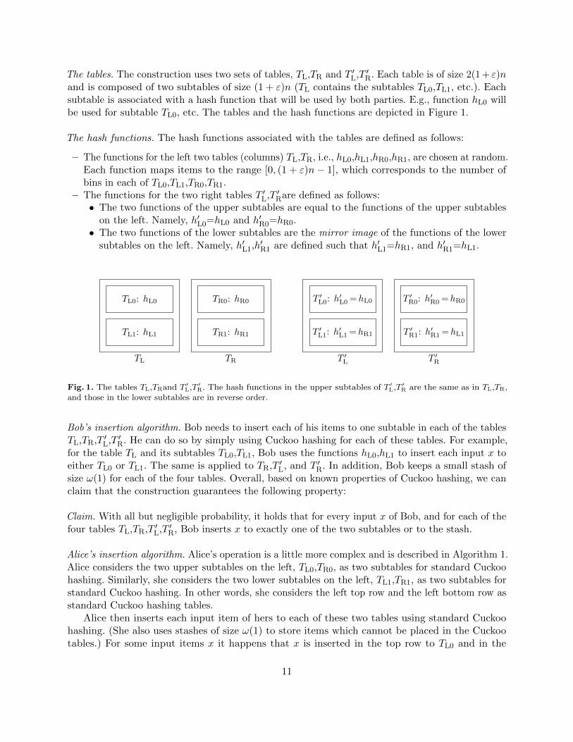


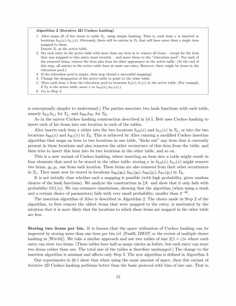
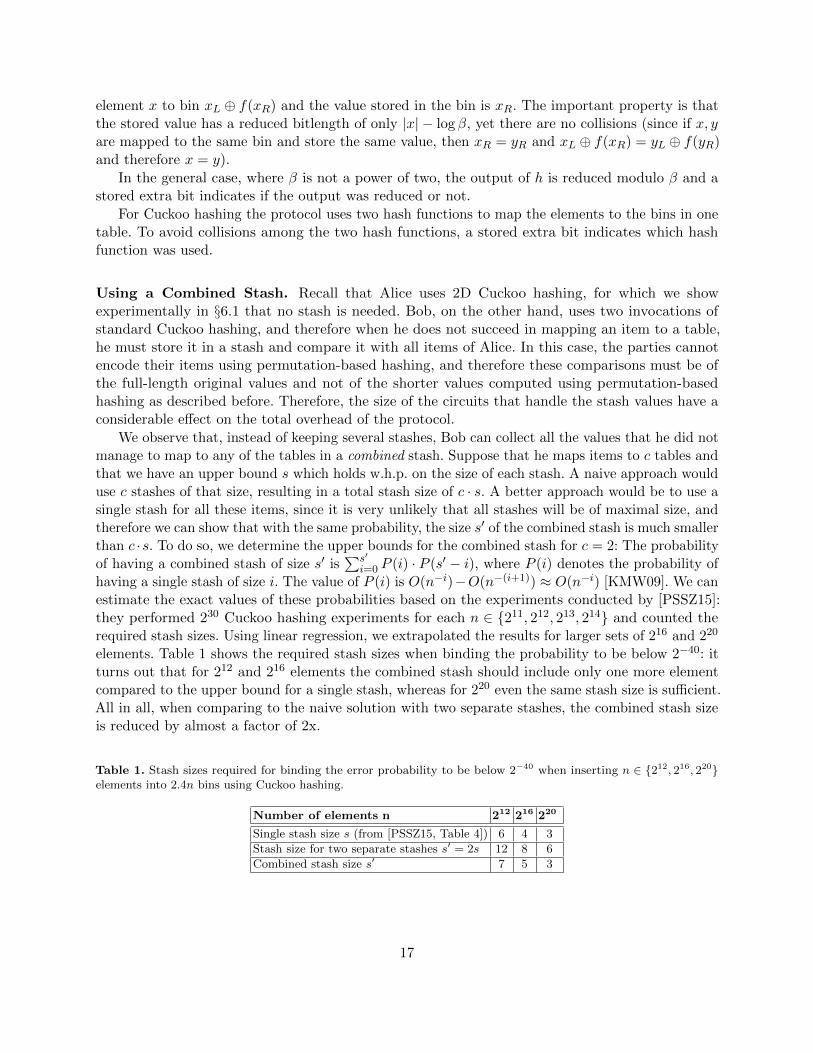


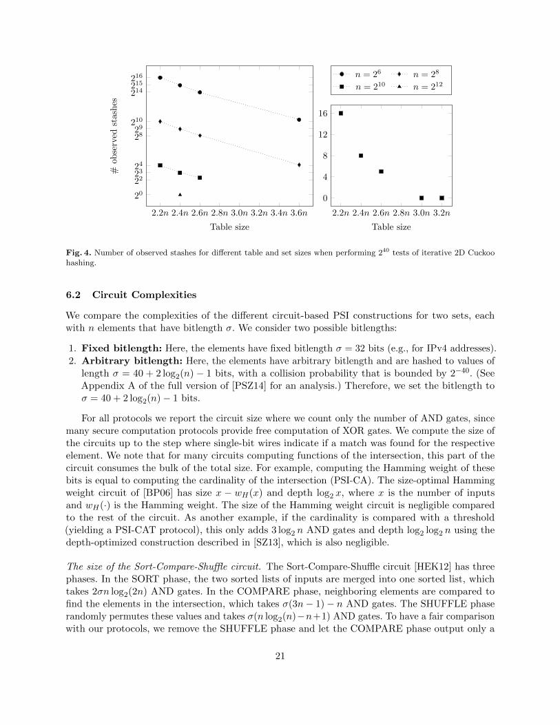
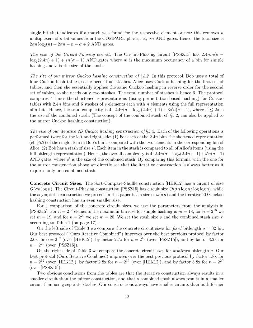


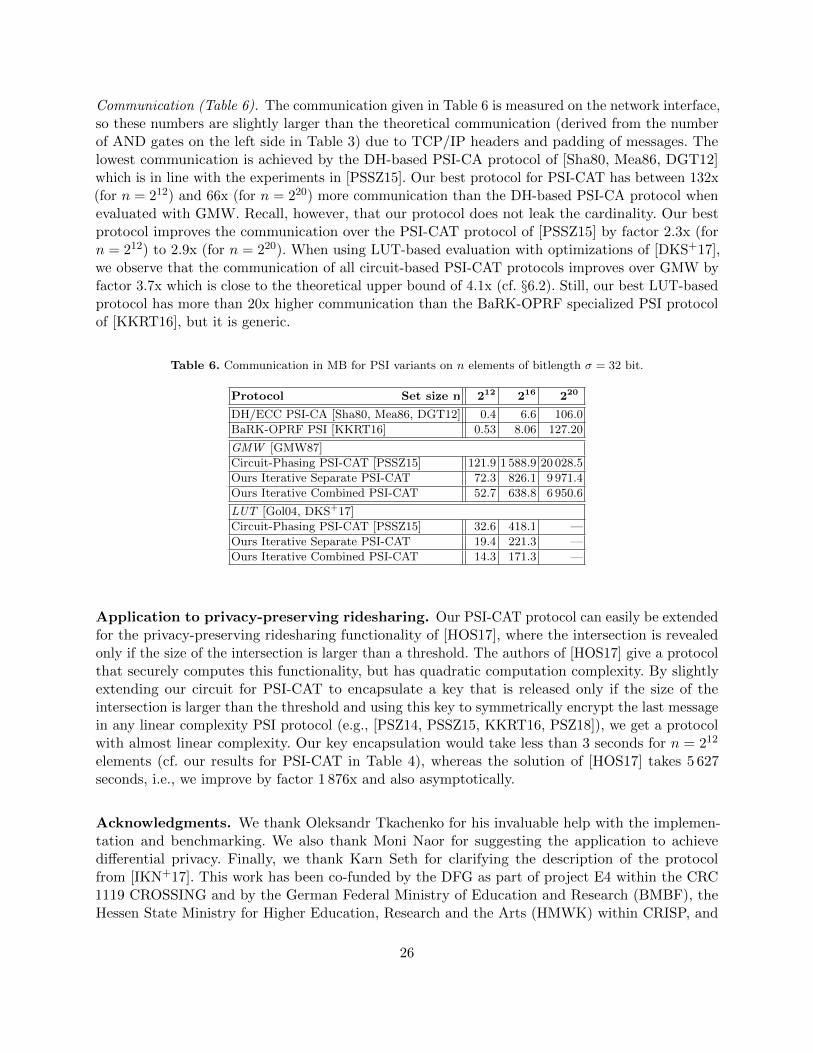


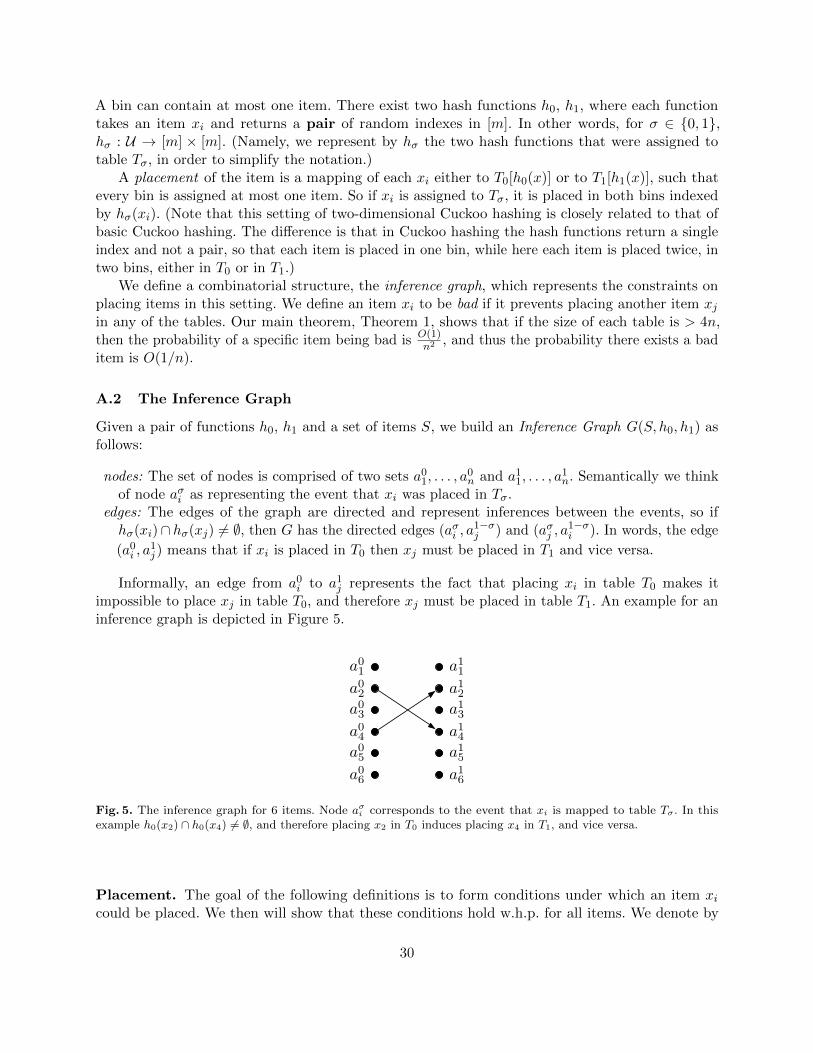
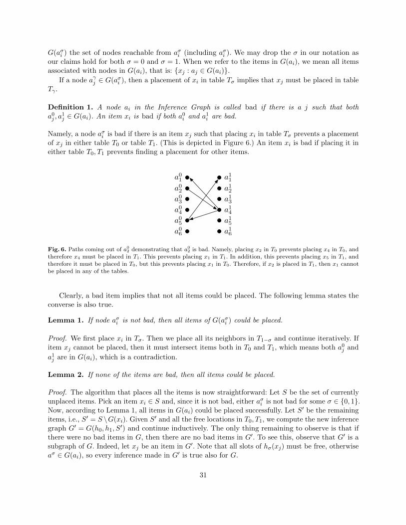


![Maximum Bipartite Matching Size And Application to Cuckoo Hashingdhay/publications/Kanizo10HK.pdf · 2010-10-17 · model of cuckoo hashing [16,27,34]. We provide again an exact expected](https://static.documents.pub/doc/80x56/5f3b8a8540c3ef7caf4f5f36/maximum-bipartite-matching-size-and-application-to-cuckoo-dhaypublicationskanizo10hkpdf.jpg)


