T H E E U R O M O N E Y

I N T E R N AT I O N A L D E B T C A P I TA L M A R K E T S H A N D B O O K

20 0 4

A S P E C I A L R E V I E W BY M O H A M O U D D U A L E H A N D A B U K A R A L IY I E L D C U R V E . C O M

A standardised interest-rate swap contract

247

Standardised

INTEREST-RATE SWAPS:assessing the LIFFE Swapnote®

by Mohamoud Dualeh and Abukar Ali, YieldCurve.com

The ubiquitous interest-rate swap has proved itself, over some notinconsiderable time, to be one of the great success stories offinancial derivatives. It is arguably the most widely-traded derivativecontract and has lent itself to constant development and application.Its flexibility derives in part from its over-the-counter (OTC)bespoke nature. Paradoxically, financial institutions have alsoconsidered that an exchange-traded swap contract, transacted alongsimilar lines to exchange-traded futures, may present uniqueadvantages in combining some of the flexibility of the OTC swapwith the usefulness of standardised contracts.

Thus financial institutions have in recent years

considered a new class of interest-rate futures products –

the exchange-traded swap contract. On March 20, 2001

LIFFE launched Swapnote®. The Swapnote® contract is

essentially a forward starting swap contract that cash

settles on the start/effective date of the underlying swap.

Following its introduction, trading volume in this

instrument can now be considered liquid. The success of

the Swapnote® is due to its simplicity in creating a

standardised exchange-traded futures contract but

combining the price sensitivity of an interest-rate swap.

As such it can be used for a variety of hedging and

trading purposes.

In this article we explore some methods of evaluating

Swapnote® futures. First, we consider briefly the take-up

of Swapnote®. We look at evaluating Swapnote® using

one of the standard interest rate models. We then

consider briefly the standard method for computing the

convexity adjustment necessary when using the contract

for cash market hedging, before concluding the article.

SWAPS AND A NEW BENCHMARK

The Swapnote® has introduced a new dimension to the

interest-rate swap market. Swapnote® is a family of

futures contracts that allows institutions to access the

euro interest-rate swaps market. It is dependent on the

euro swap yield curve, usually simply called the swap

curve. In terms of notional volume the swap market is

the largest fixed income market in the world, being

approximately six times the size of the bond market.1

A standardised interest-rate swap contract

In an era of diminishing liquidity in government bond

markets, and the advent of the euro, the swap market has

become the benchmark for long-term interest rates.

Hence the swap curve has become the primary means of

price discovery in the euro-denominated fixed income

market. The factors which contributed to this included

the size and homogeneity of the swap market, compared

to combined government bond markets, and the decline

in government bond issuance, together with growing

non-government and corporate bond issuance.2 The

turnover of the swap market on the other hand,

consistently trends upwards, for instance it grew by

104% between 1998 and 2001.3

From a trader’s point of view, the best hedges are

achieved through vehicles that are highly liquid and as

closely correlated with the underlying assets as possible.

In Europe (and arguably in other markets) the interest

rate swaps market now appears to achieving this better

than the government debt markets. The efficacy of the

swap curve as a benchmark reflects the fact that the euro

swaps market is now larger than the Eurozone

government bond market.

Exchange-traded swap contracts are traded on the

London International Financial Futures and Options

Exchange (LIFFE) and the Chicago Board of Trade (CBOT).

Both are based on the future value of a swap rate. The

Swapnote® futures contracts have grown rapidly since

their introduction in March 2001. For traders and investors

with exposure to credit risk based on Libor, the Swapnote®

contract has been accepted as an effective hedging tool as,

for instance, the US Treasury futures contract does not

take credit risk into account. Hedging a swap portfolio

with government bonds appears to work extremely well,

however the assumption that the bond-swap spread

remains constant is, in practice, not realistic. The spread

often exhibits significant volatility.4 In fact, hedging with

government bond futures presents significant basis risk.

The Swapnote® is designed to both strengthen the

benchmark status of the swap curve and provide an

effective and accessible hedge for a portfolio of securities.

It should also reduce basis risk for practitioners looking to

hedge (say) corporate bond portfolios.

THE SWAPNOTE® CONTRACT

For readers reference we provide first an overview of the

main features of the Swapnote® contract. Swapnote® is

essentially a forward starting swap contract that cash

settles on the start or effective date of the underlying swap.

The contract can also be regarded as a cash-settled bond

futures contract with a single notional bond in the

deliverable basket. The contract is essentially similar to a

standardised exchange-traded futures contract but with the

price sensitivity of an interest rate swap. Each Swapnote®

contract has a series of notional cash-flows underlying it

comprising a fixed coupon element together with a

principal repayment such that it replicates a notional bond.

At first, the coupon level is set at 6% for each of the

contracts, thereby facilitating spread trading between

government bond futures contracts and Swapnote®

contracts of related maturity. Similarly the contracts are

timed on a quarterly expiry cycle for the months of

March, June, September and December, the usual expiry

months for futures exchanges, and denoted by the letters

H, M, U and Z. Exhibit 1 illustrates the 10-year

Swapnote® contract specification.

Swapnote® is a standardised exchange-traded futures

contract. In other words, the 10-year swap futures will

all be in the same contract month. With Swapnote®, if

we assume that there is sufficient liquidity5 it may be

easier to execute a buy or sale of 10-year swap futures

than it currently is to buy or sell a 10-year strip of

Eurodollar futures contracts.

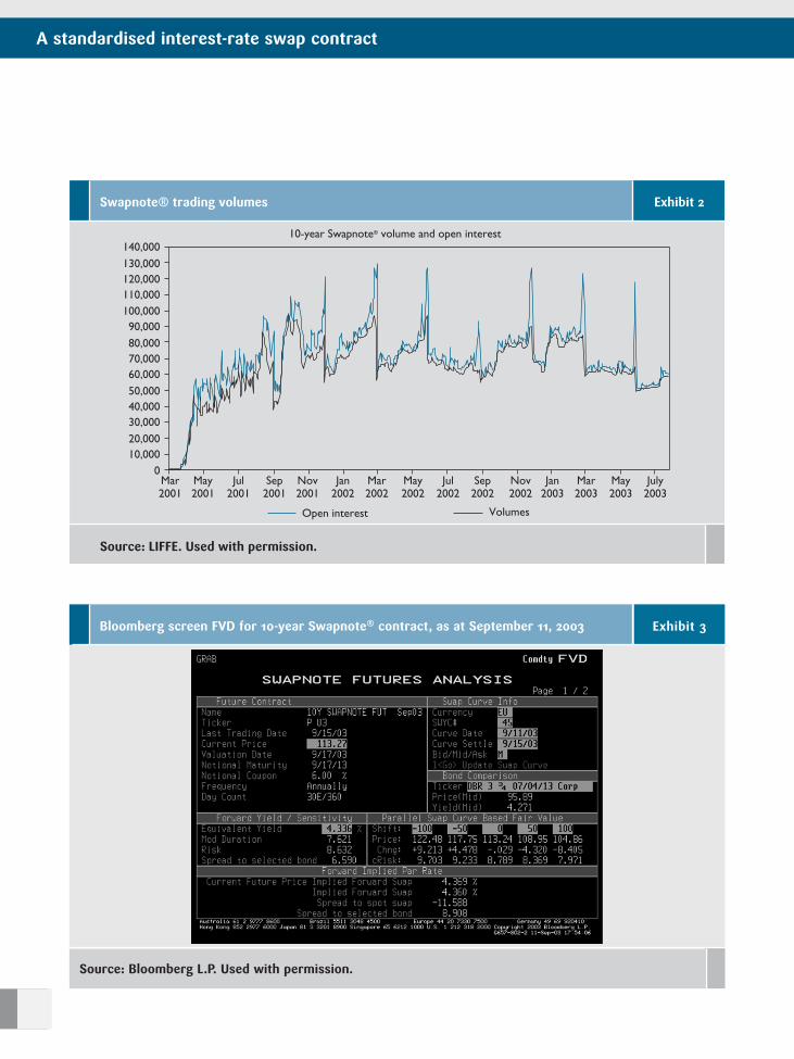
We show trading volumes for the Swapnote® futures

contract in Exhibit 2. During 2003 volumes experienced

new highs, with the 10-year contract recording a daily

volume high of 55,261 in June 2003 (June 13, 2003) and

the five-year contract setting a new volume high record

of 57,761 in the same month.6

A standardised interest-rate swap contract

247

EVALUATING THE SWAPNOTE® CONTRACT

The price of the Swapnote® contract until its expiration

date will reflect underlying supply and demand risk

factors. At expiration, the contract settles based on the

Exchange Delivery Settlement Price (EDSP) fixed by the

exchange. The EDSP is defined as the sum of the

discounted notional cash-flows, each of which has been

present valued using zero coupon discount factors

derived from the ISDA Benchmark Swap Rates on the

last trading day. The discount factors are zero coupon

rates bootstrapped from the current par swap curve.

Cash-flow payment dates are defined as anniversary

dates of the effective date. However, should any of these

dates fall on weekend or holiday, notional cash-flows are

moved to a business day.

Users of the Bloomberg system can use the Bloomberg

Swapnote® Futures Analysis function, screen FVD, to

evaluate the fair value of a Swapnote® contract, which is

illustrated in Exhibit 3. It is obtained by typing

P A Cmdty FVD <GO>.

Screen FVD (see Exhibit 3) shows the market value of the

Swapnote® and its conventions such as the day count and

valuation date. The Swapnote® can be priced as a forward

starting swap where the swaps effective date is set as the

valuation date of the futures contract. The sensitivity

measures from the FVD screen can be replicated by pricing

a 10-year euro-denominated bond with a forward

settlement date of the futures valuation date and maturity

date, day count and frequency from the futures contract.

Note from Exhibit 3 that a 6% notional coupon is used as

the bond's fixed coupon rate. In our example we have

evaluated the 10-year Swapnote®. Exhibit 4 is page 2 from

the same screen, and lists the fixed coupon and forward

rates at each interest fixing date. The forward rates as at

10-year Swapnote® - contract specification Exhibit 1

Source: LIFFE

€100,000 notional principal amount

Notional coupon6.0%

Maturities 2Notional principal amount due 10 years from thedelivery day

Delivery months March, June, September and December such that thenearest two delivery months are always available fortrading

Delivery day Third Wednesday of the delivery month

Last trading day 11:00 Brussels time (10:00 London time)Two London business days prior to the delivery day

QuotationPer €100 nominal value

Minimum price movement(Tick size and value)0.01(€10)

Trading hours on LIFFE CONNECT™07:00 - 18:00

A standardised interest-rate swap contract

Exhibit 2Swapnote® trading volumes

Source: LIFFE. Used with permission.

010,00020,00030,00040,00050,00060,00070,00080,00090,000

100,000110,000120,000130,000140,000

Mar2001

May2001

Jul2001

Sep2001

Nov2001

Jan2002

Mar2002

May2002

Jul2002

Sep2002

Nov2002

Jan2003

Mar2003

May2003

July2003

Open interest Volumes

10-year Swapnote® volume and open interest

Bloomberg screen FVD for 10-year Swapnote® contract, as at September 11, 2003 Exhibit 3

Source: Bloomberg L.P. Used with permission.

each fixing date are also shown. Screen FVD assesses

Swapnote® against a comparison bond. This defaults to the

current 10-year German government bond, shown to be the

3.75% 2013 bond. The ‘equivalent yield' shown is the

notional yield to maturity of a government bond with a 6%

yield priced to settle on the valuation date, and maturing

exactly 10 years from the valuation date. The spread to the

comparison bond is shown to be 6.59 basis points.

The Swapnote® delivery method is cash settlement. The

final settlement value will be determined as

X *[6/r + (1 - 6/r)*(1 + 0.01*r/2)-20]. (1)

The underlying notional cash-flows consist of a series

of fixed notional coupons and a notional principal at

maturity, the dates of which fall on anniversaries of the

delivery day. Once the cash-flows from futures contract

are implicit, any of the standard interest rate models can

be used to price Swapnote® contracts.7

Of course it is not essential that a proper term-structure

model should be used. Fundamentally, the Swapnote®

quoted price corresponds to the forward value of a bond

having a 6% coupon. At maturity, the settlement price is

computed by discounting the 6% coupons plus principal

using a zero coupon curve derived from the official swap

rate fixings.

To illustrate, using linear interpolation we priced the

two-year, five-year and 10-year Swapnote®s. First we

constructed a zero curve off deposit and swap rates and

discounted the coupons and the notional principal of the

underlying swap. From Exhibit 5 we show the quoted

prices and our theoretical prices. Note that we converted

those into equivalent bond yields to get a difference in

term of basis points. In fact we can do the same analysis

using Bloomberg.

We reiterate that the Swapnote® contract is essentially a

forward starting swap contract that cash settles on the

start/effective date of the underlying swap. Thus, a swap

247

A standardised interest-rate swap contract

Bloomberg screen FVD, page 2 Exhibit 4

Source: Bloomberg L.P. Used with permission.

A standardised interest-rate swap contract

position can be interpreted as a package of

forward/futures contracts. Future contracts are designed to

remove the risk of default8 inherent in forward contracts.

Through the device of marking to market9, the value of the

future contract is maintained at zero at all times. Thus,

either party can close out his/her position at any time.

This difference gives rise to the convexity bias. When

hedging or pricing across futures and swaps markets, the

issue of the convexity bias will lead to hedge risk.

If one is pricing the Swapnote® as a forward starting

swap using the swap curve, then there is no issue: the

swap curve already exhibits a convex feature. Hence

there is no need to adjust for the convexity effect. If

however one wishes to price the swap off the Euribor

futures contracts, then one will need to adjust the curve

defaults for convexity bias. The Bloomberg Swapnote®

Futures calculator does not adjust for convexity because

it uses the market swap curve (see Exhibit 3) and not the

curve derived from futures contracts to calculate the

implied forward rates needed when pricing swaps.

Therefore, when using the Euribor futures, the back

month futures do not reflect the true Euribor forward

rates and the volatility of rates required for valuing

swaps. To overcome the imperfections in hedging that

this will cause, one must adjust for this bias. The

simplest approach is to use one of the standard interest

rate models but with a convexity adjustment.

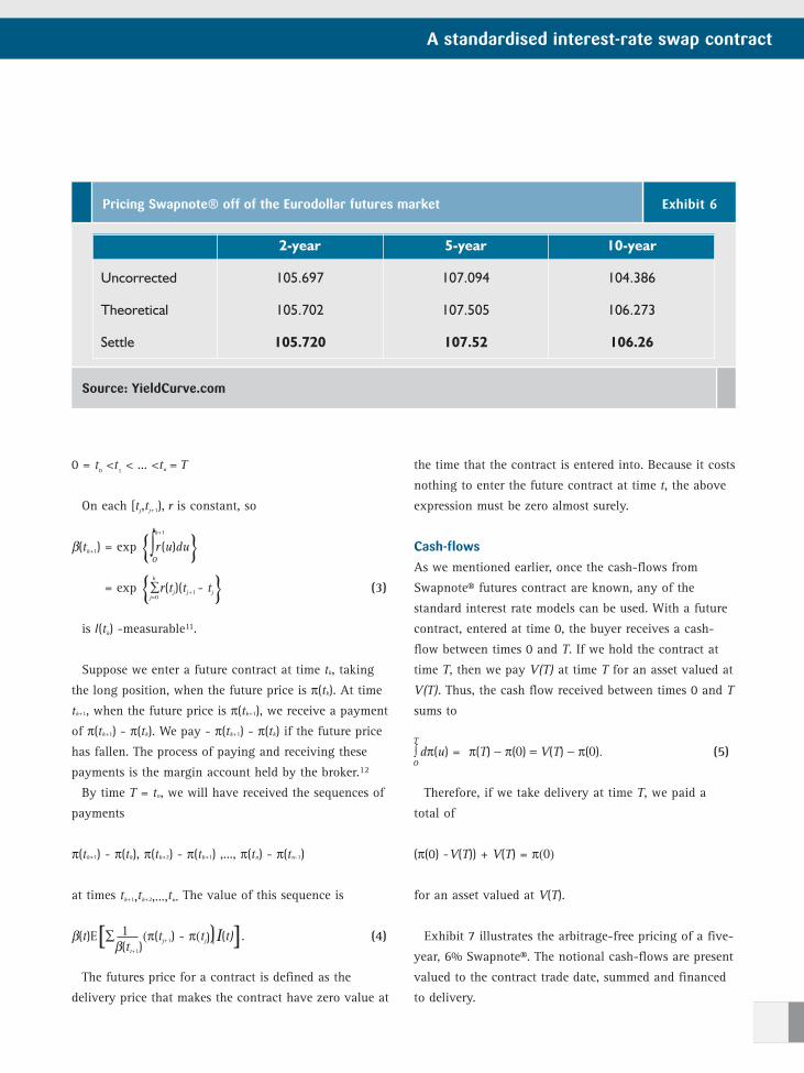
In Exhibits 5 and 6 we are comparing the Swapnote®

settlement prices with those of the Euribor futures

which settle at around the same time. The main

difference between these methods of evaluating the

Swapnote® is that the last method takes into account

the convexity correction discussed below. Exhibit 6

illustrates pricing Swapnote® off the Eurodollar futures

market using the LIFFE Swapnote® calculator, together

with a convexity correction using the Kirikos & Novak

equation. We look at this issue in greater detail later.

PRICING FRAMEWORK

We can now formulate the framework that leads to the

standard methodology for pricing the Swapnote®

contract. Let us start first by defining the accumulation

factor (i.e. the saving account) as

β(t ) = exp [∫r(u)du] (2)

A zero coupon bond, maturing at time T, pays US$1

at time T and nothing before time T10. Intuitively,

Equation (2) represents the price process of a risk-free

security which continuously compounds in value at the

rate r. We first consider the situation with discrete

trading dates

Comparison of quoted and theoretical prices Exhibit 5

Source: YieldCurve.com

2-year 5-year 10-year

Quoted 106.06750 110.46000 113.52500

Theoretical 106.07138 110.46619 113.51066

t

0

0 = t0<t

1< ... <tn = T

On each [tj,tj+1), r is constant, so

β(tk+1) = exp {∫r (u)du}= exp {∑r(tj)(tj+1 - tj} (3)

is I(tk) -measurable11.

Suppose we enter a future contract at time tk, taking

the long position, when the future price is π(tk). At time

tk+1, when the future price is π(tk+1), we receive a payment

of π(tk+1) - π(tk). We pay - π(tk+1) - π(tk) if the future price

has fallen. The process of paying and receiving these

payments is the margin account held by the broker.12

By time T = tn, we will have received the sequences of

payments

π(tk+1) - π(tk), π(tk+2) - π(tk+1) ,..., π(tn) - π(tn-1)

at times tk+1,tk+2,...,tn. The value of this sequence is

β(t)E[∑ 1 (π(tj+1) - π(tj))|I(t)]. (4)

The futures price for a contract is defined as the

delivery price that makes the contract have zero value at

the time that the contract is entered into. Because it costs

nothing to enter the future contract at time t, the above

expression must be zero almost surely.

Cash-flows

As we mentioned earlier, once the cash-flows from

Swapnote® futures contract are known, any of the

standard interest rate models can be used. With a future

contract, entered at time 0, the buyer receives a cash-

flow between times 0 and T. If we hold the contract at

time T, then we pay V(T) at time T for an asset valued at

V(T). Thus, the cash flow received between times 0 and T

sums to

∫ dπ(u) = π(T) − π(0) = V(T) − π(0). (5)

Therefore, if we take delivery at time T, we paid a

total of

(π(0) -V(T)) + V(T) = π(0)

for an asset valued at V(T).

Exhibit 7 illustrates the arbitrage-free pricing of a five-

year, 6% Swapnote®. The notional cash-flows are present

valued to the contract trade date, summed and financed

to delivery.

247

A standardised interest-rate swap contract

Pricing Swapnote® off of the Eurodollar futures market Exhibit 6

Source: YieldCurve.com

2-year 5-year 10-year

Uncorrected 105.697 107.094 104.386

Theoretical 105.702 107.505 106.273

Settle 105.720 107.52 106.26

k

j=0

β(tt+1)

T

0

tk+1

0

A standardised interest-rate swap contract

Forward – future spread

Earlier we suggested an interpretation of a swap as a

package of forward/futures contracts, given that we can

now look at the forward/futures spread.13 First let us

define the future price and the forward price.14

Future price: π(t) = E[V(T)|I(t)].

Forward price:

We can derive the difference between the forward bond price

by using a zero-coupon curve and the future bond price.

Let be the discount factor until time T.15

The forward – future spread is

(6)

If and V(T) are uncorrelated, then π(0) - F(0).

Assuming that V(T) and are perfectly correlated,

then we have, using last expression of Equation (6), and

rearranging

(7)

Therefore, the forward –future spread is given by

Forward - Futures Spread = (8)

β(T) denotes the saving account value at time T (for

US$1 invested at time 0) and V(T) the value of the asset

considered at time T .

Exhibit 7Arbitrage-free pricing of a five-year, 6% Swapnote®

Source: YieldCurve.com

6%xAF1 6%xAF2 6%xAF3 6%xAF4

100 + 6xAF5

Trade date Contractdelivery date

V(t) V(t)F(t) = =B(t,T) 1β(t)E[β(T) |I(t)]

V(0)π(0) - F(0) = E[V(T )] -1

E[β(T)]

E ( 1 )β(T)

1 1 V(T) = [E(β(T))E(V(T)) - E (β(T))]1E (β(T))

1β(T)

1β(T)

V(T ) 1 1E(β(T) ) = E (β(T)) E(VT )+σV(T )*σ(β(T))

1 1(β(T))*σV(T )*σ (β(T))

To calculate the standard deviation of β(T) and V(T) it is

best to use the one factor Hull-White model because other

standard interest rate models such as Black Karasinski,

Black-Derman-Toy and Cox-Ingerosll-Ross are more

knotty.16 Basically the core difference between the models is

skew, and the convexity correction is mainly an at-the-

money phenomenon which is not very sensitive to skew.17

Thus, the H&W model is less opaque and compute intensive.

In the next section we consider the convexity correction.

Convexity adjustment estimation

A tailed hedge for the money market swap possesses a

very desirable property, namely the net value of the swap

plus hedge is positive irrespective of rates going up or

down. Earlier we derived the forward/futures spread to

be zero. However, if the futures position is greater (i.e.

gaining) than the forward position, then as

compensation, there must be an adjustment. There are

several approaches of measuring the convexity effect (i.e.

the convexity bias in futures)18, but the Kirikos and

Novak equation using Hull and White is a robust

treatment for the convexity correction. For a rate that

applies between time t and time T, under the Hull and

White model the difference between the forward and

futures rates is expressed as the z parameter of the

popular Kirikos & Novak equation.19

Convexity adjustments for several futures markets are

provided by brokers or from market data vendors.

Estimating the convexity adjustment requires an

estimation of the future path of interest rates up to the

future contract maturity. In the Hull-White model, the

continuously compounded forward rate, lasting between

times t and T (denominated in years from current date),

equals the continuously compounded future rate with the

following adjustment factor eZ. Of course this is the

Kirikos & Novak factor,

where Z = Λ + Φ

adjusts for the fact that the

underlying is an interest rate, and

where σ is the standard deviation of the change in short-

term interest rates expressed annually, and a is the mean

reversion rate.

Convexity bias estimation requires an estimate of the

mean reversion rate (a) and the standard deviation (σ) of

the change in short-term interest rates expressed

annually. For simplicity, LIFFE assumes a constant

default value for the mean reversion speed. The LIFFE

US$ Swapnote® calculator assumes that the mean

reversion parameter (a) remains at 0.03. Bloomberg does

allow convexity adjustment for pricing swaps if the

underlying interest rate curve is based on traded futures

contracts. There are two input parameters that are

required in order to adjust futures contracts for

convexity: the mean reversion speed which has a default

level of 0.03 and volatility parameters which are fed

from market traded implied cap/floor rates. There are

various alternative methodologies for estimating the

volatility parameters (σ and a). The two most popular

methodologies are:

• to estimate the volatility parameters from prices of

traded securities; and

• as discussed above, a deposit/swap derived curve

could be used to estimate the volatility parameters.

CONCLUSION

Hedging a swap portfolio with government bond curves

presents significant basis risk. A futures contract

referenced to the swap curve provides a far more effective

hedging tool with appreciably reduced basis risk. To

address the problem of basis risk one can use a Swapnote®

contract. The usefulness of Swapnote® as a hedging tool

includes the ability to match and hedge credit exposures

with a derivative instrument that closely correlates with

that exposure. The capacity to hedge swap book exposures

and avoidance of convexity, plus avoidance of problems

247

1 - e-2at 1 - e-a(T-t) 2Λ = σ2 ( 2a )[ a ]

σ2 1 - e-a(T-t) 1 - e-at 2Φ = 2 ( a )[ a ]

A standardised interest-rate swap contract

A standardised interest-rate swap contract

that can be associated with government bond contracts

under adverse market conditions, are key advantages.

The Swapnote® has allowed institutional investors to

access the euro interest rate swaps market in standardised

fashion. It is simple to price, once the cash flows from

futures contracts are known. Any of the standard interest

rate models can be used to evaluate the contract. The

futures/forward spread can be adjusted using the Kirikos

& Novak equation.

Finally we have shown how the convexity bias

adjustment can be effected by following a straightforward

approach and which will allow Swapnote® to be applied

across futures and swaps markets for effective hedging.

Notes:

1. Source: ISDA, “Summary of OTC Derivative Market Data”, www.isda.org/statistics.

2. A number of other factors have contributed to this, resulting in greater use of the swap

curve to as the euro Benchmark. For a general discussion of government bond market

illiquidity and the issues behind alternative benchmarks, see Choudhry (2003).

3. Source: www.isda.org/statistics. For a good discussion and related issues see Remolona and

Wooldridge (2003).

4. See Flavell (2001), chapter 9 for more discussion about how the optimal hedge effectiveness

in this regard can be rather low.

5. From anecdotal evidence the authors conclude that there is sufficient liquidity in the

market. However given the relative youth of this instrument, this cannot be assumed to be

permanent and continued observation would be prudent.

6. The authors express thanks to Kumud Chavda from LIFFE for providing these figures.

7. For instance, the Black 76, Cox-Ingersoll-Ross, Black-Derman-Toy and Hull-White models, to

mention a few.

8. The default risk in a swap agreement is the counterparty risk.

9. That is, at end of each trading day, the margin account is adjusted to reflect the investors

gain or loss.

10. Our approach follows that of Shreve (1997). There are number of sources on derivatives

instruments that one can access on this issue, for instance Hull (2000). For mathematics of

derivatives we refer the reader to Shreve (1997).

11. Some authors write I(t) as F(t), it is matter of choice!

12. A good reference about the margin requirement is Fabozzi (2003).

13. Basically we can view the swap spread as the futures/forward spread.

14. It is important to keep in mind that futures affect the swap through both estimation and

discounting process.

15. Until expiry

16. There is no closed form solution for these models. You could use Monte Carlo simulation for

example to calculate the payments along each path and discount them back.

17. Thanks to Patrick Hagan for pointing this out. See Hagan (2003).

18. See Richard Flavell, Swaps and Other Derivatives, Wiley (2000), pp 185-203.

19. See G. Kirikos and D. Novak (1997). This is also available at www.powerfinance.com/convexity

References:

Choudhry, M., “Illiquidity in government bond markets and the search for alternative

benchmarks”, Department of Management Working Paper, Birkbeck, University of

London 2003

Fabozzi, F., Valuation of Fixed Income Securities and Derivatives, 3rd Edition, John Wiley 2003

Flavell, R., Swaps and other Derivatives, John Wiley 2001

Hagan, P., “Convexity conundrums: Pricing CMS Swaps, Caps and Floors” Wilmott

Magazine, March 2003 pp 38-44

Hull, J., Options, Futures, and Other Derivatives, 4th Edition, FT Prentice Hall 2000

Kirikos, G., and Novak, D., “Convexity conundrums” RISK, March 1997, pp 60-61

Remolona, E., Wooldridge, P., “The euro interest rate swap market”, BIS Quarterly

Review, March 2003

Shreve, S., Lectures on Stochastic Calculus and Finance (1997), available at

www-2.cs.cmu.edu/~chal./shreve.html

Moorad Choudhry, co-founder of YieldCurve.com

Mohamoud Dualeh and Abukar Ali

YieldCurve.com

For further information, please

e-mail: info@yieldcurve.com

247

YieldCurve.com is the specialist fixed income and derivatives market research website

and e-Journal. It produces cutting edge research and development in the field of

capital markets products, financial engineering and quantitative analysis. Its

Associates are a mix of investment banking professionals and published authors in

leading finance and economics Journals.

The website contains articles and presentations on a wide range of topics on finance

and banking. In addition there are training aids, transcripts and video files of

conference presentations and television appearances by YieldCurve.com associates, as

well as software packages for a range of applications including yield curve

modelling, derivatives pricing and hedging, and Monte Carlo simulations.

Group membership and corporate sponsorship packages are available for

market practitioners.

www.YieldCurve.com

info@yieldcurve.com

YieldCurve.publishing is the only publisher working exclusively in the field of fixed

income, derivatives and financial engineering.

A standardised interest-rate swap contract