Effective Conductivity of Spiral and other Radial

Symmetric Assemblages

Andrej CherkaevDepartment of Mathematics, University of Utah

andAlexander D. Pruss

Department of Mathematics, Duke University

June 20, 2012

Keywords: Effective Medium theory, Spiral assemblage, exact effective prop-erties, composite models.

Abstract

Assemblies of circular inclusions with spiraling laminate structure in-side them are studied, such as spirals with inner inclusions, spirals withshells, assemblies of ”wheels” - structures from laminates with radially de-pendent volume fractions, complex axisymmetric three-dimensional micro-geometries called Connected Hubs and Spiky Balls. The described assem-blages model structures met in rock mechanics, biology, etc. The classicaleffective medium theory coupled with hierarchical homogenization is used.It is found that fields in spiral assemblages satisfy a coupled system of twosecond order differential equations, rather than a single differential equa-tion; a homogeneous external field applied to the assembly is transformedinto a rotated homogeneous field inside of the inclusions. The effectiveconductivity of the two-dimensional Star assembly is equivalent to that ofHashin-Shtrikman coated circles, but the conductivity of analogous three-dimensional Spiky Ball is different from the conductivity of coated spheregeometry.

1 Introduction

Structures with explicitly computable effective properties play a specialrole in the theory of composites. They allow for testing, optimizing, anddemonstrating of dependences on the structural parameters and materialproperties. These structures are also used for hierarchical modeling ofmore complicated structures and they permit explicitly computing fieldsinside the structure and track their dependence on structural parameters.There are several known classes of such structures: the Hashin-Shtrikmancoated spheres structure [6] and Schulgasser’s structures [11] are probably

1

arX

iv:1

206.

3604

v2 [

mat

h-ph

] 2

0 Ju

n 20

12

the most investigated geometries of composites. The scheme has been gen-eralized to multiscale multi-coated spheres (see the discussion in [4, 8]),coated ellipsoids [3], and the ”wheel assembly”, studied in [1]. Anotherpopular class is laminate structures and derivatives of them, the laminateof a rank, which exploit a multiscale scheme in which a course scale lam-inate is made from smaller scale laminates in an iterative process. Thelimits of iterations of these structures yields to a differential scheme wherean infinitesimal layer is added at each step, see [4, 8].

In the present paper, we combine the idea of multi-rank laminates andcoated spheres, introducing assemblies of circular inclusions with spiralinglaminate structure inside them. Namely, we study the assemblages of spi-rals with inner inclusions, spirals with shells, and assemblies of ”wheels” -structures from laminates with radially dependent mass fractions. We alsoderive the effective conductivities of complex three-dimensional microge-ometries, which we call Connected Hubs and Spiky Balls. The describedstructures model inhomogeneous materials met in rock mechanics, biol-ogy, etc. For calculating effective properties, we use the classical effectivemedium theory, see [6, 8, 9, 10]) coupled with hierarchical homogeniza-tion. We study spiral assemblies with inclusions and observe an interest-ing phenomenon: a homogeneous external field applied to the assemblyis transformed into a rotated homogeneous field inside of the inclusions.The fields in such structures satisfy a coupled system of two second or-der differential equations, rather than a single differential equation that issatisfied in Hashin-Shtrikman and Schulgasser’s structures. We show thatthe effective conductivity of the two-dimensional Star is equivalent [1] toconductivity of Hashin-Shtrikman coated circles, but the conductivity ofthe analogous three-dimensional Spiky Ball is different from the coatedspheres geometry.

2 Composite circular inclusion

Consider an infinite conducting plane with coordinates (x1, x2) and as-sume that a unit homogeneous electrical field e = (1, 0)T is applied to theplane at infinity, inducing a potential u,

lim||x||→∞

u(x) = x1. (1)

A structured circular inclusion of unit radius ‖x‖ ≤ 1 is inserted in aplane. It consists of a core inner circle of radius r0 and an envelopingannulus. The inner circle (nucleus) Ωi = x : ||x|| < r0 ≤ 1, is filled withan isotropic material of conductivity σi. The annulus Ωa = x : r0 <||x|| < 1 is filled with anisotropic material whose conductivity tensorSe(r) depends only on radius. The plane outside the inclusion is denotedΩ∗, it is filled with an isotropic material of conductivity σ∗.

Effective conductivity of such an assembly is computed by effectivemedium theory. Given the inclusion, we find the conductivity σ∗ so thatthe inclusion is cloaked,

u(x) = x1 if ||x|| > 1. (2)

2

If this is the case, the outer conductivity σ∗ is called the effective conduc-tivity of the inclusion. The inclusion is not seen by an outside observer,therefore the entire plane can be filled with such inclusions, according toeffective medium theory [6, 8, 9, 10].

We show that the field inside the nucleus Ωi has the representation

u = ρ (cos(ψ)x1 + sin(ψ)x2) , ||x|| < r0 (3)

where ρ, ψ are constant. An observer inside Ωi records a homogeneousfield similar to the outside field, but rotated by an angle ψ.

The current j, electric potential u, and electric field e in a conductingmedium are related by equations

∇ · j = 0, e = ∇u, j = K e, (4)

where K is a positively defined symmetric conductivity tensor that rep-resents the material’s properties. In our assemblage,

K =

σiId if x ∈ ΩiSe if x ∈ Ωaσ∗Id if x ∈ Ω∗

,

Here, Id is the identity matrix. Equations (4) are combined as a conven-tional second order conductivity equation

∇ ·K∇u = 0. (5)

On the boundaries between different regions, tensor K is discontin-uous. But the potential u, the normal current j · n, and the tangentialpotential e · t are continuous,

[u]+− = 0, [j · n]+− = 0, [e · t]+− = 0, (6)

where [.]+− denotes the jump. For instance, at the boundary of the nucleus,we have

[u]+− = limε→0,ε>0

u(r + ε, θ)− u(r − ε, θ).

3 Fields in a spiral assemblage

In this section we find the fields, currents, and effective conductivity ofthe described assemblage assuming that the eigenvectors of K in Ωa forma family of logarithmic spirals. We call the resulting structure the Spiralwith Core.

Single Inclusion. Rewrite the problem in polar coordinates r, θ.Solving conductivity equation (5), we find that the potential in the innerand outer isotropic regions is

u(r, θ) = Ar cos(θ) +B r sin(θ) if 0 ≤ r < r0 (x ∈ Ωi)u(r, θ) = r cos(θ) if r > 1, (x ∈ Ω∗)

(7)

A,B are constants. The form of the solution in the outer domain reflectsthe effective medium condition: the inclusion is invisible, and field isunperturbed and agrees with condition (2).

3

Figure 1: Spiral with Core

Assume that the angle φ of orientation of the principle axes of K inΩa to the radius is constant, so that the eigendirections form a family oflogarithmic spirals. In Ωa, K has the form

K =

[Krr Krθ

Krθ Kθθ

]= RSeR

T ,

where

R =

[cos(φ) sin(φ)− sin(φ) cos(φ)

], Se =

[σ1 00 σ2

].

σ1 and σ2 are positive constant eigenvalues of Se, and φ is the angle ofthe spiral. The entries of K are:

Krr = σ1 cos2(φ) + σ2 sin2 φ,Krθ = (σ1 − σ2) cos(φ) sin(φ)Kθθ = σ1 sin2(φ) + σ2 cos2(φ)

Equation (5) in the annulus becomes(1

r

∂

∂rr[Krr

∂

∂r+Krθ

1

r

∂

∂θ

]+

1

r

∂

∂θ

[Krθ

∂

∂r+Kθθ

1

r

∂

∂θ

])u(r, θ) = 0

(8)We separate variables and account for boundary conditions. The solutionhas the form

u(r, θ) = U(r) cos(θ) + V (r) sin(θ).

and U and V satisfy a system of ordinary differential equations

L1U − L2V = 0, L1V + L2U = 0 (9)

where L1 and L2 are linear differential operators,

L1 =(d

drrKr

d

dr− 1

rKθθ

), L2 = −

(d

drKrθ +Krθ

d

dr

). (10)

Notice that equations in (9) are respectively the real and complex part ofa complex-valued differential equation

(L1 + iL2)(U + iV ) = 0 (11)

Write the current in the spiral as j = Ju cos(θ)+Jv sin(θ). We compute

Ju = KrrdU

dr+Krθ

V

r, Jv = Krr

dV

dr−Krθ

U

r. (12)

4

The jump conditions (6) at r = r0 and r = 1 have the form

[U ]+− = 0, [V ]+− = 0, [Ju]+− = 0, [Jv]+− = 0. (13)

Potentials U, V in annulus Ωa are found by solving (9):

U = rα(C1 cos(β)− C2 sin(β)) + r−α(C3 cos(β)− C4 sin(β)), (14)

V = rα(C1 sin(β) + C2 cos(β)) + r−α(C3 sin(β) + C4 cos(β)), (15)

where

α =√σ1σ2, β =

ln(r)Krθ

Kr.

Determination of Constants. Jump conditions (13) at the outerboundary (r = 1) are

C2 + C4 = 0, C2 − C4 = 0 (16)

yielding C2 = 0, C4 = 0. There remain five unknown constants, k∗, C1, C3, A,and B. They appear to be overdetermined by the remaining six bound-ary conditions. However, the four boundary conditions (13) on the innerboundary at r0 can be reduced to just three conditions, allowing the sys-tem to solved.

The potentials U and V in the spiral material are linked together,and knowing either one is sufficient to determine the other. Indeed, uponsubstituting C2 = 0, C4 = 0, we find

V (r) = U(r) tan(β(r)) (17)

dV (r)

dr=dU(r)

drtan(β(r)) +

U(r)(1 + tan2(β(r)))Krθ

rKr. (18)

Substituting this into (12), we see that the same relationship holds for thenormal components of the current,

Jv = KrdU(r)

drtan(β(r)) +

U(r)

rKrθ tan2(β(r)) = Ju tan(β(r), (19)

so we have, in the spiral,

V (r)

U(r)=Jv(r)

Ju(r)= tan(β(r)). (20)

Using (20), the current conditions (13) are redundant, as the two con-ditions on the current are simultaneously satisfied. The four boundaryconditions can be rewritten as three,

[U ]+− = 0, [V ]+− = 0, tan(β(r0)) =B

A. (21)

With this observation, the linear system can be solved for the remain-ing unknowns. Among them is the effective conductivity of the outerregion, σ∗, which is treated as an unknown. Notice that the annulus withspiraling material does not perturb the outside field, and contains a ho-mogeneous inner field that is directed in a different direction than theouter homogeneous field.

5

The value of σ∗ is obtained by solving the system is the effective con-ductivity of the structure; it is given by an explicit formula

σ∗ =σ2σ1(rγ0 − 1) + σi

√σ1σ2(rγ0 + 1)

σi(rγ0 − 1) +

√σ1σ2(rγ0 + 1)

, (22)

where

γ =2√σ1σ2

sin(φ)2σ1 − sin(φ)2σ2 − σ1.

Figure 2: Spiral Assemblage

Effective Medium Theory. The Spiral with Core structure, asdescribed above, extends from the origin to a radius of one. But thisradius is arbitrary in an infinite plane. The spiral can be scaled up ordown with respect to the radius and will still solve the same problem. Asthe spiral leaves the outside field unperturbed, placing multiple spirals sideby side will result in every object placed being rendered invisible to thefield, with each having an inner homogeneous field directed in a differentdirection than the applied field. While none of the myriad inclusions aredetectable by perturbations of the outside field, the field is differentlydirected almost everywhere.

4 Extreme Spiral Geometries

Extremal Spiral Angle. By design, the core of the spiral object containsa uniform electric field directed in a different direction than the outsidefield. The potential in inner region (nucleus) has the representation

u(r, θ) = Ar cos(θ) +Br sin(θ).

The field inside will make an angle of Υ = tan−1(B/A) with the uniformfield outside the spiral. A and B depend on the spiral angle φ, so a

6

substitution shows Υ = γ|σ2 − σ1|, where

γ =ln(r0) cos(φ) sin(φ)

sin2(φ)σ1 − sin2(φ)σ2 − σ1

. (23)

Let us find the angle φ which maximizes the rotation Υ. A straight-

Figure 3: Changing Direction of the Electric Field

forward calculation shows that for a given σ1 and σ2, Υ is maximized bychoosing

φ0 = arctan(√σ1/σ2). (24)

The maximal angle Υmax for a given σ1, σ2, and r0 is

Υmax = −1

2ln(r0)

∣∣∣σ1

σ2− 1

∣∣∣√σ2

σ1. (25)

Here, r0 ≤ 1, the radius of inclusion. It’s clear that the more anisotropicthe spiral and the smaller the inner radius r0 are, the larger the resultingtwist inside the spiral’s core is.

Laminates. The conductivities σ1, σ2 in (25) describe the conductiv-ities of the outer spiral material in the Spiral with Core structure. If thisanisotropic material is a laminate made of materials with conductivitiesk1, k2 and volume fractions m1,m2, then σ1, σ2 can be written as thegeometric and arithmetic means of the conductivities,[4]

σ1 = m1k1 +m2k2, σ2 =(m1

k1+m2

k2

)−1

. (26)

For given materials with conductivities k1, k2, we can optimize Υ withrespect to m1,m2. The maximal angle of rotation is obtained for

m1 = m2 =1

2. (27)

It is equal to

Υmax = −1

4ln(r0)

(k1 − k2)2

(k1 + k2)√k1k2

(28)

7

In particular, Υ = π (and the current inside goes in the opposite direction)if

ln(r0) = −4π

√k1k2(k1 + k2)

(k1 − k2)2. (29)

For instance, if k1 = 1 and k2 = 100, the inner field will be directedopposite to the external field when r0 = 0.274.

Values of Υ greater than 2π are also possible. The relative anglebetween the incident current and the inner current is the value of Υ takenmod 2π.

5 Derivative Assemblages

The parameters in the Spiral with Core structure can be modified toobtain effective conductivity of similar conducting assemblages.

Hashin-Shtrikman Coated Circles. The classical example of theHashin-Shtrikman geometry[3] is an isotropic circle surrounded by anisotropic annulus

Figure 4: Left: Coated Circles. Right: Schulgasser’s Geometry (orange slice)

It is obtained from the Spiral with Core by setting σ1 = σ2. Theouter spiral layer becomes an isotropic shell, and the effective conductivitycoincides with Hashin-Shtrikman’s result

khs = σ1(σi + σ1) + r20(σi − σ1)

(σi + σ1)− r20(σi − σ1). (30)

Notice that m = r20 is the volume fraction of the core material.Schulgasser Structure. Schulgasser [11] suggested another clas-

sical symmetric geometry . It is a radial laminate of two materials.Schulgasser’s structure is obtained from the Spiral with Core by settingr0 = 0, φ = 0. The inner isotropic circle disappears and the logarith-mic spiral laminate is straightened into a radial laminate. The effectiveconductivity agrees with [11].

ksch =√σ1σ2. (31)

Orange with Core. This object has an inner circle of isotropicmaterial surrounded by an annulus made up of a radial laminate.

The Orange with Core is obtained from the Spiral with Core by set-ting φ = 0. The logarithmic spiral laminate is straightened into a radiallaminate. The effective conductivity of the Orange with Core is

8

Figure 5: Left Orange with Core. Right: Orange with Shell

kc = σ1

σiκ(1 + r2κ0

)+ σ2

(1− r2κ0

)σ1κ (1 + r2κ0 ) + σi (1− r2κ0 )

, κ =

√σ2

σ1. (32)

Note that this formula can be written in terms of volume fractions byobserving that the volume fraction mi of the inner material is mi = r20.

Orange with Shell. This object contains an inner radial laminatesurrounded by an isotropic material. Denote the conductivity of the outerisotropic shell by σ1, and the conductivity tensor (in polar coordinates)for the inner laminate by

K =

[σr 00 σθ

]The effective conductivity can be found by a straight calculation. It is

ks = σ1

√σθσr(r

20 + 1) + σ1(1− r20)

√σθσr(1− r20) + σ1(r20 + 1)

. (33)

Indeed, the material in an inner circle is a Schulgasser radial laminate,which has effective property k∗ =

√σrσθ. Thus, this inner material can

be treated as an isotropic material with conductivity√σrσθ. The effective

property of the Orange with Shell can be obtained by substituting σi =√σrσθ into the equation for the effective property of Hashin-Shtrikman

coated circles.Basic Spiral. This object is simply the spiral material centered

around the origin.

Figure 6: Left: Basic Spiral. Right: Spiral with Shell

The Basic Spiral can be obtained from the Spiral with Core by settingr0 = 0. The effective conductivity of the spiral is

ksp =√σ1σ2. (34)

9

As one might expect, it coincides with the effective conductivity of Schul-gasser’s geometry.

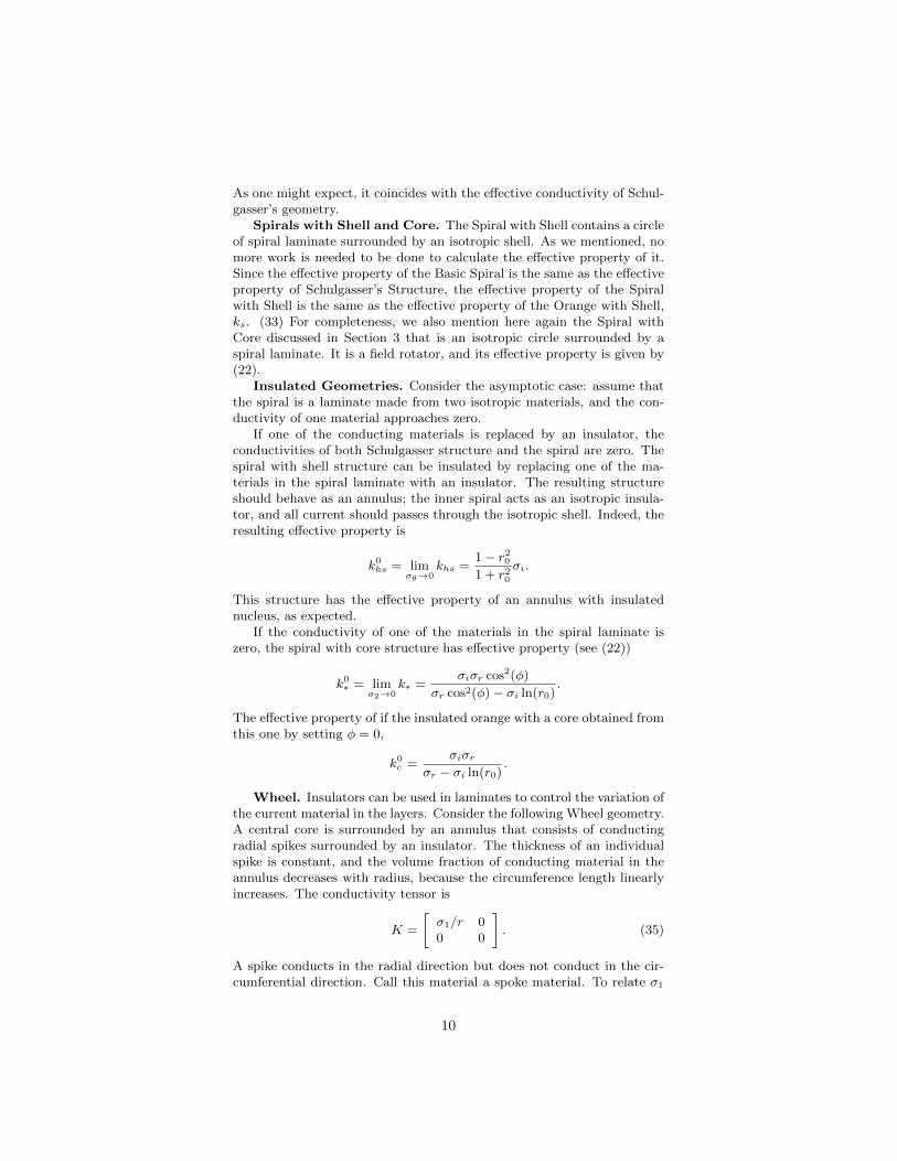
Spirals with Shell and Core. The Spiral with Shell contains a circleof spiral laminate surrounded by an isotropic shell. As we mentioned, nomore work is needed to be done to calculate the effective property of it.Since the effective property of the Basic Spiral is the same as the effectiveproperty of Schulgasser’s Structure, the effective property of the Spiralwith Shell is the same as the effective property of the Orange with Shell,ks. (33) For completeness, we also mention here again the Spiral withCore discussed in Section 3 that is an isotropic circle surrounded by aspiral laminate. It is a field rotator, and its effective property is given by(22).

Insulated Geometries. Consider the asymptotic case: assume thatthe spiral is a laminate made from two isotropic materials, and the con-ductivity of one material approaches zero.

If one of the conducting materials is replaced by an insulator, theconductivities of both Schulgasser structure and the spiral are zero. Thespiral with shell structure can be insulated by replacing one of the ma-terials in the spiral laminate with an insulator. The resulting structureshould behave as an annulus; the inner spiral acts as an isotropic insula-tor, and all current should passes through the isotropic shell. Indeed, theresulting effective property is

k0hs = limσθ→0

khs =1− r201 + r20

σi.

This structure has the effective property of an annulus with insulatednucleus, as expected.

If the conductivity of one of the materials in the spiral laminate iszero, the spiral with core structure has effective property (see (22))

k0∗ = limσ2→0

k∗ =σiσr cos2(φ)

σr cos2(φ)− σi ln(r0).

The effective property of if the insulated orange with a core obtained fromthis one by setting φ = 0,

k0c =σiσr

σr − σi ln(r0).

Wheel. Insulators can be used in laminates to control the variation ofthe current material in the layers. Consider the following Wheel geometry.A central core is surrounded by an annulus that consists of conductingradial spikes surrounded by an insulator. The thickness of an individualspike is constant, and the volume fraction of conducting material in theannulus decreases with radius, because the circumference length linearlyincreases. The conductivity tensor is

K =

[σ1/r 00 0

]. (35)

A spike conducts in the radial direction but does not conduct in the cir-cumferential direction. Call this material a spoke material. To relate σ1

10

to the conductivity σ of the spoke material, we can write σµr0 = σ1. Theparameter µ ∈ [0, 1] shows the relative thickness of the spikes at the radiusr0.

This time we are dealing with a material with anisotropic conductivitythat varies with radius. The solution to the potential inside the spokematerial satisfies (5). The current is constant inside each spoke, thereforethe potential is

u = (Ar +B) cos(θ) + (Cr +D) sin(θ). (36)

The wheel inclusion has an inner isotropic core and an outer isotropicshell, connected by spokes. It conductivity depends on radius as follows

Figure 7: Left: Wheel. Right: Star

K =

σiId if r < r0[σ1/r 00 0

]if r0 < r < r1

σ2Id if r1 < r < 1σ∗Id if r > 1

. (37)

Since the potentials in each region are known, a procedure similar tothat in Section 3 gives that the effective conductivity of the Wheel:

kwheel = σ2A+B

B −A, (38)

where

A = r21σ1σi + r21r0σ2σi − r21σ1σ2 − r31σ2σi,

B = riσiσ2 + σ2σ1 + σ1σi − r0σ2σi.

When r1 → 1, the outer conducting layer disappears and we come tothe structure that we call Star. Its effective conductivity is

kst =σiσ1

σ1 + σi(1− r0). (39)

Star assemblages can model structures of hubs connected by conductingstrands in an insulating space. If the conductor in inner circles and spokeis the same, σi = σ, we write the effective property σstar in terms of thevolume fraction m of conducting material σ,

kstar(r0,m) =σm(r0)

2−m(r0), where m(r0) = r20 + 2µr0(1− r0). (40)

11

If µ = 12, then r0 = m and kstar coincides with the effective con-

ductivity of coated circles, therefore it is an optimal structure for theresistivity minimization problem [1] along with the coated circles [6]. Thevalue µ = 1

2makes intuitive sense. One can see that if the spokes in the

Star cover only half the circumference of the inner sphere at r0, then thecurrent density in the isotropic region of the star will be half that in thespokes region of the star. If two orthogonal currents are separately appliedto the Star structure, the sum of their energy density is constant through-out the structure. This satisfies a necessary and sufficient condition forminimization of resistivity [4]

6 3D radially symmetric assemblages

The same approach can be applied to three-dimensional radially symmet-ric inclusions. Let us consider spherical inclusions, embedded in an infinitethree-dimensional isotropic conducting material with undetermined con-ductivity. A uniform electric field is applied to the plane. The equation(5) is used to solve for the potential in each material. The boundary con-ditions (6) are similar to the two-dimensional case. Applying a uniformcurrent along the z-axis results in the electric potential

u = ρ cos(φ) (41)

outside the inclusion. This solution is obtained by separation of variablesin equation (5) in spherical coordinates.

Hub. We construct an analogue of the two-dimensional spoke mate-rial, which consists of radial spokes of constant thickness. The relativeproportion of conducting material is inversely proportional to the squareof the radius, and the tensor in spherical coordinates is

K =σµρ20ρ2

[1 0 00 0 00 0 0

]. (42)

We choose µ ∈ [0, 1] so that the term µρ20 is the surface area covered bythe spikes at the inner radius ρ0.

The solution for the potential inside this material is

u = (C1 + C2ρ) cos(φ). (43)

Using this material, we construct a Hub structure. The Hub is the three-dimensional analog of the two-dimensional Star structure. It model in-clusions spread through an insulating space and connected by conductingstrands. The Hub consists of an inner isotropic core of conductivity σiout to a radius of ρ, enveloped by a spoke material.

The effective conductivity of the Hub is computed similarly to that ofStar. It depends on two structural parameters, ρ0 and µ and is equal to

khub =σiσρ

20µ

σi(1− ρ0) + σµρ0. (44)

The volume fraction of the Hub is

12

Figure 8: Left: Hub. Right: Spiky Ball.

m = r30 + 3µr20(1− r0). (45)

If, by analogy with the star, we take µ = 13, this relation gives r20 = m,

and the effective conductivity is

khub =σm

3− 2√m. (46)

Unlike the two-dimensional case, this conductivity is different from theconductivity of coated spheres.

Spiky Ball. The Spiky Ball structure is a generalized hub, in whichthe spikes have variable cross-section. The tensor of this generalized ma-terial is

K =σµρn0ρn

[1 0 00 0 00 0 0

]. (47)

The effective conductivity of this assemblage is

ksb =σiσρ

n0µ(n− 1)

σi(1− ρn−10 ) + σµρn−1

0 (n− 1). (48)

Notice that the Spiky Ball, Hub, and Star require that the currentpasses sequentially through insulated spokes and a homogeneous centralcircle (sphere). Because of this, their effective conductivity are of har-monic mean type,

1

k∗=a

σ+

b

σi, (49)

where a and b are constants depending only on the geometry.

7 Conclusion

In constructing the Spiral with Core structure, we constructed a fieldrotator, e.g. a conducting structure that rotates an incident uniform elec-tric field while remaining undetectable. Optimization results show how tomaximize the angle of rotation induced by this field rotator. By modifyingthe Spiral with Core, a large number of other conducting structures can beconstructed and their effective conductivities computed. The analogous3D Hub and 2D Star structures behave differently in the sense that the

13

2D star corresponds to minimal effective conductivity while the 3D Hubdoes not.

Acknowledgement The work was supported by NSF through grantDMS 0707974.

References

[1] A. Cherkaev. Optimal Three-Material Wheel Assemblage of Con-ducting and Elastic Composites arXiv:1105.4302 [math-ph] 22 May2011

[2] N. Albin, A. Cherkaev, V. Nesi. Multiphase laminates of extremaleffective conductivity in two dimensions. Journal of the Mechanicsand Physics of Solids, Volume 51, Issue 10, October 2003, Pages1773-1813.

[3] Y. Benveniste and G.W. Milton, New Exact Results for the Effec-tive Electric, Elastic, Piezoelectric and other Properties of CompositeEllipsoid Assemblages, J. Mech. Phys. Solids, 51, 1773-1813, 2003.

[4] A. Cherkaev. Variational methods for structural optimization, Chap-ter 2. Springer Verlag NY 2000

[5] R. M. Christensen, Mechanics of Composite Materials. Wiley NY1979

[6] Z. Hashin, S. Shtrikman, A Variational Approach to the Theory ofthe Effective Magnetic Permeability of Multiphase Materials. AppliedPhysics 33, 3125 (1962).

[7] P. Lipinskia, El H. Barhadia, M. Cherkaouib. Micromechanical mod-elling of an arbitrary ellipsoidal multi-coated inclusion. PhilosophicalMagazine, Volume 86, Issue 10, 2006.

[8] G. W. Milton, The Theory of Composites. Campridge UniversityPress, 2001.

[9] S. Nemat-Nasser, M. Hori. Micromechanics: Overall Properties ofHeterogenous Materials. Elsevire, NY 1999

[10] J. A. Reynolds and J. M. Hough. Formulae for Dielectric Constantof Mixtures 1957 Proc. Phys. Soc. B 70 769

[11] K. Schulgasser. Sphere assemblage model for polycrystals and sym-metric materials, Journal of Applied Physics, 54, 3, 1380-1382,(1983).

[12] S. Torquato. Effective stiffness tensor of composite media-I. Exactseries expansions. Journal of the Mechanics and Physics of Solids,Volume 45, Issue 9, September 1997, Pages 1421-1448

14