○E

The Earthquake-Source InversionValidation (SIV) Projectby P. Martin Mai, Danijel Schorlemmer, Morgan Page, Jean-PaulAmpuero, Kimiyuki Asano, Mathieu Causse, Susana Custodio, WenyuanFan, Gaetano Festa, Martin Galis, Frantisek Gallovic, Walter Imperatori,Martin Käser, Dmytro Malytskyy, Ryo Okuwaki, Fred Pollitz, LucaPassone, Hoby N. T. Razafindrakoto, Haruko Sekiguchi, Seok Goo Song,Surendra N. Somala, Kiran K. S. Thingbaijam, Cedric Twardzik, Martinvan Driel, Jagdish C. Vyas, Rongjiang Wang, Yuji Yagi, and Olaf Zielke

ABSTRACT

Finite-fault earthquake source inversions infer the (time-depen-dent) displacement on the rupture surface from geophysicaldata. The resulting earthquake source models document thecomplexity of the rupture process. However, multiple sourcemodels for the same earthquake, obtained by different researchteams, often exhibit remarkable dissimilarities. To address theuncertainties in earthquake-source inversion methods and tounderstand strengths and weaknesses of the various approachesused, the Source Inversion Validation (SIV) project conducts aset of forward-modeling exercises and inversion benchmarks. Inthis article, we describe the SIV strategy, the initial benchmarks,and current SIV results. Furthermore, we apply statistical toolsfor quantitative waveform comparison and for investigatingsource-model (dis)similarities that enable us to rank the solu-tions, and to identify particularly promising source inversion ap-proaches. All SIV exercises (with related data and descriptions)and statistical comparison tools are available via an online col-laboration platform, and we encourage source modelers to usethe SIV benchmarks for developing and testing new methods.We envision that the SIV efforts will lead to new developmentsfor tackling the earthquake-source imaging problem.

Online Material: Figures of velocity-density structure, source-receiver geometries, slip-rate functions, input and inverted rup-ture models, quantitative waveform comparisons. Tables of scalarsource parameters and dissimilarity values.

INTRODUCTION

Finite-fault earthquake-source inversions infer the spatiotemporalrupture evolution on one or more fault planes using geologic

information, seismic and/or geodetic data, and potentially in-cluding also (or using exclusively) tsunami measurements. Sourceinversions provide important information on the complexity ofthe earthquake rupture process. Earthquake source-scaling studiesuse finite-fault information to determine rupture parameters fordeveloping empirical scaling laws that shed light on earthquakemechanics (Somerville et al., 1999; Mai and Beroza, 2000; Maiet al., 2005; Manighetti et al., 2005; Blaser et al., 2010; Strasseret al., 2010). Researchers use the space–time-dependent sourceinversion results to develop spontaneous dynamic rupture modelsand to work toward a general understanding of earthquake rup-ture physics (e.g., Heaton, 1990; Bouchon, 1997; Ide and Takeo,1997; Day et al., 1998; Page et al., 2005; Tinti et al., 2005; Maiet al., 2006; Gabriel et al., 2012; Causse et al., 2013). For indi-vidual earthquakes, source studies reveal cascading failure of com-plex fault systems (Yue et al., 2012) or rerupturing of thehypocentral region (Lee et al., 2011). Thus, finite-fault inversionsprovide the key for discerning earthquake source complexity.

A quantitative understanding of rupture complexity is alsoessential for ground-motion prediction studies that require anadequate characterization of slip heterogeneity to generate real-istic scenario earthquakes (e.g., Mai, 2009). Slip-heterogeneitycharacterizations are based on source models of past earth-quakes (e.g., Mai and Beroza, 2002; Lavallée et al., 2006;Causse et al., 2010; Gusev, 2011; K. K. S. Thingbaijam andP. M. Mai, unpublished manuscript, 2016). Inference on rup-ture speed and its variation (e.g., Archuleta, 1984; Dunhamand Archuleta, 2004; Bouchon et al., 2010) provide evidencefor the occurrence of supershear rupture velocity, which is criti-cal not only for realistic ground-motion simulations, but alsofor understanding the dynamic rupture process. Finite-faultslip maps are also needed to compute postmainshock stress

690 Seismological Research Letters Volume 87, Number 3 May/June 2016 doi: 10.1785/0220150231

changes that can be related to the aftershock activity (Kinget al., 1994; Stein et al., 1997).

Much of our understanding of earthquake source com-plexity stems from finite-source rupture models, building onthe pioneering work of Olson and Apsel (1982). A detailedreview of source inversion techniques is beyond the scope ofthis article; instead we refer to Ide (2007). To illustrate the generalconcept, we use the representation theorem (Aki and Richards,2002) written asEQ-TARGET;temp:intralink-;df1;52;637

un�x; t� �Zdτ

ZZΣ�si�ξ;τ��× cijpq × vj ×Gnp;q�x; t − τ;ξ;0�dΣ;

�1�in which �si�ξ; τ�� represents the slip velocity at locations ξ andtimes τ, cijpq is the elasticity tensor, vj is the vector normal to thefault surface Σ, and Gnp;q denotes the medium response to thegeneralized force couple in the xq direction with force in the pdirection. un�x; t� is the nth component of the ground-motiontime series at location x. The representation theorem in equa-tion (1) describes a linear relation between the rupture processsi�ξ; τ� on the fault and the observed displacement un�x; t�.For practical purposes, Earth structure, fault–receiver geometry,and the force-couples responses are combined into the Green’sfunction G�x; ξ; t�. When solving the inverse problem, we seeka kinematic parameterization of the space–time-dependent rup-ture process (e.g., discrete basis functions for the slip-rate distri-bution si�ξ; τ�) that minimizes the differences between recordedgroundmotions and the predictions (computed using equation 1).In principle, equation (1) results in a linear inverse problem, butone that is inherently underdetermined. To solve it, one mustreduce the dimension of the model space to make the problemoverdetermined, for instance through regularization of the solu-tion by applying a spatial and/or temporal operator (or both).

For computational purposes, the rupture surface in equa-tion (1) is discretized into small elements (called subfaults) inwhich the kinematic rupture process is parameterized using oneor more elementary slip-rate functions. Each of these subfaultsis activated as the rupture front sweeps over the fault planewith rupture speed vr . In slip inversions, vr is often assumedconstant, in which case the inversion is run several times atdifferent values of vr to find the optimal vr that leads tothe minimum misfit. A linear multi-time-window source inver-sion applies more than one elementary slip-rate function torepresent the rupture evolution on a single subfault. Rupturespeed vr may be spatially variable, which can be achieved bysolving for the rupture-onset time at each subfault. Typically,this is done using a nonlinear inversion approach. When usingthe discretized form of equation (1) for earthquake-source in-version, the inferred rupture model depends also on the chosendiscretization, parameterization, and misfit function, as well ason the particular method for solving the inverse problem.

Many source inversion methods have been proposed, ei-ther as constrained linear inversions (e.g., Olson and Apsel,1982; Hartzell and Heaton, 1983) or nonlinear inversions thatsearch the model space without stringent constraints (e.g.,Hartzell et al., 1996; Liu and Archuleta, 2004; Monelli and

Mai, 2008). These inversions use seismic data (strong-motion,teleseismic; e.g.,Wald et al., 1991; Yoshida et al., 1996), geodeticmeasurements (to constrain fault geometry and the final staticdisplacement; e.g., Jónsson et al., 2002), or a combination ofboth, potentially augmented with information on surface rup-ture or other constraints (e.g., Asano et al., 2005). Slip duringlarge tsunamigenic megathrust earthquakes can be constrainedby tsunami waveform data (e.g., Satake et al., 2013). Recently,Gallovic et al. (2015) developed a regularized linear inversionthat is unconstrained in the temporal rupture evolution. Therequired Green’s functions G�x; ξ; t� are computed using a va-riety of techniques and parameterizations of the Earth’s crust(layered 1D models, full 3D models; e.g., Graves and Wald,2001; Wald and Graves, 2001), whereas some methods use smallearthquakes as empirical Green’s functions (Dreger, 1994).

Earthquake-source inversions provide tools and models toinvestigate earthquake rupture processes and have become analmost routine analysis for studying rupture kinematics. Forlarge and important earthquakes, near-real-time finite-faultsource inversions are available online only a few hours afterthe event (e.g., Hayes, 2011). Results of many finite-fault stud-ies are collected in the online SRCMOD database (Mai andThingbaijam, 2014; see also Data and Resources). However,the resolution and robustness of these finite-fault rupture mod-els is not well understood. For instance, significant differencesare seen for rupture models of the same earthquake but inferredby different researchers. Figure 1 shows four slip models for the1999 Mw 7.6 İzmit earthquake (out of six solutions in theSRCMOD database) that are strikingly different. The discrep-ancies in these slip distributions have been described previously(Beresnev, 2003; Ide et al., 2005) and may be attributed to(1) differences in the data selection and processing; (2) themethods used for computing the Green’s functions for eachdataset; (3) the assumed Earth structure, fault geometry, andother geophysical parameters; and (4) the method and param-eterization for the inversion itself (linearized or fully nonlinearinversion; spatial and temporal discretization; applied smooth-ing and regularization). Items (2–3) are directly related to us-ing equation (1).

Because of our imperfect knowledge of Earth’s structure andfault geometry, and because of insufficient data, the source inver-sion problem is nonunique: many rupture-model solutions mayfit the data equally well. Also, rigorous uncertainty quantificationin earthquake source studies is needed but, unfortunately, is oftenneglected. An ensemble of solutions is obtained when varyinginversion input parameters and processing steps to investigatethe corresponding model sensitivities (e.g., Custódio et al., 2005;Konca et al., 2013; Liu et al., 2006; Hartzell et al., 2007). Baye-sian approaches provide a more formal way to quantify rupture-model uncertainties (Monelli et al., 2009; Duputel et al., 2012;Minson et al., 2013), but estimating the full posterior probabilitydensity functions of the inverted source quantities is computa-tionally still demanding (e.g., Bernauer et al., 2014; Dettmer et al.,2014; Razafindrakoto and Mai, 2014).

To better understand the limits and robustness of earth-quake-source inversion methods, and to examine how the

Seismological Research Letters Volume 87, Number 3 May/June 2016 691

different steps of the source inversion workflow (steps 1–4,above) affect the rupture-model results, the earthquake SourceInversion Validation (SIV) initiative was launched (Page et al.,2011). The SIVproject extends a previous source inversion test-ing study (Mai et al., 2007) and seeks to develop new methodsfor uncertainty quantification in earthquake source inversions.A long-term goal of the SIV initiative is also to develop a (semi)automated source inversion platform on which variousapproaches can be tested simultaneously with minimal user in-tervention to arrive at transparent, fully testable, and reproduc-ible earthquake source models with comprehensively quantifieduncertainties.

Below, we introduce the SIV initiative, describe the strat-egy of our work, and report the results achieved so far, whichinclude newly developed inversion methods and statisticalanalysis tools that are a direct outcome of the SIVcollaboration.

STRATEGY

The workflow for finite-fault earthquake source inversions re-quires several steps, including data selection and data process-ing, choosing and running a proper forward-solver withadequate input parameterization, and conducting the actualinversion. Each of these steps influences the resulting rupturemodel. The SIV initiative tries to address all aspects of thisworkflow and to isolate their effects on the inversion results.Correspondingly, our strategy is to begin with simple forward-modeling exercises to test various Green’s function computa-tion codes and their use. Next, we define a suite of inversionbenchmarks with increasing complexity. Either certain meta-data are not specified, or only with uncertainty, or noise isadded to the synthetics. Including geometrical variations in therupture model for forward simulations adds another layer of

intricacy to the benchmarks. The Southern California Earth-quake Center (SCEC)/U.S. Geological Survey (USGS) codeverification exercise (Harris et al., 2009) follows a similar strat-egy through a set of forward-modeling problems with increas-ing complexity for testing numerical methods for dynamicearthquake rupture simulations.

To set up the inversion benchmarks, a subgroup of the SIVteam generates input (target) earthquake-rupture models withvarying degrees of source complexity for which forward sim-ulations are run to compute synthetic datasets. Depending onthe benchmark, these may comprise only near-field seismicwaveforms or also include Global Positioning System (GPS)displacements and teleseismic synthetics. The synthetic datasetsare disseminated via an online collaboration platform (see Dataand Resources). The input source model used for each bench-mark is not publicized until the exercise is officially concluded.Registered participants use the collaboration platform to sub-mit their rupture-model solutions and predicted datasets inspecific data formats. The platform provides quantitative analy-sis tools to compare inversion solutions and predicted data be-tween different participants or with respect to the knowninput model (released after the particular benchmark is con-cluded). All benchmark exercises and related data remain acces-sible such that interested scientists can use these for follow-upresearch even after the official closure date.

In the long term, we envision an automated testing center,inspired by the Collaboratory for the Study of Earthquake Pre-dictability (e.g., Zechar et al., 2010). The goal is to establish acomputational platform on which numerous source inversioncodes are applied to a large number of benchmark exercises in atransparent manner. In such a testing center, user-driven deci-sions are replaced by algorithmically derived parameter selec-tions to generate testable and reproducible source inversions

▴ Figure 1. Selected finite-source rupture models for the 1999 Mw 7.6 İzmit earthquake (Turkey), obtained using different inversionstrategies and different datasets. Black stars mark the hypocenter. Colors indicate fault slip (in meters). Note the pronounced dissimi-larities of the slip distributions for this event. The inversion results are from (a) Bouchon et al. (2002), (b) Sekiguchi and Iwata (2002),(c) Delouis et al. (2002), and (d) Yagi and Kikuchi (2000).

692 Seismological Research Letters Volume 87, Number 3 May/June 2016

with proper uncertainty quantification (e.g., Mesirov, 2010;Eddy et al., 2012; Lees, 2012).

Next, we describe the forward-modeling exercises and in-version benchmarks of the SIVproject (summarized in Table 1).We then introduce the statistical comparison tools that the SIVplatform provides and discuss their use to assess the solutionquality and to develop a ranking scheme. Based on the resultsobtained so far, we provide a summary and set of recommen-dations for earthquake-source inversion studies and the con-tinuation of the SIV project.

FORWARD-MODELING EXERCISES

To test numerical methods for Green’s function calculations insource inversion studies, we conduct two sets of forward-mod-eling exercises for the near-fault region. We first examinepoint-source synthetics for near-field seismic waves, and thenwe test the methods with respect to precisely specified finite-fault rupture models.

Near-Source Green’s Function ComputationWe consider two point-source cases: a purely left-lateral strike-slip event on a vertical fault and a reverse-faulting event on a 40°dipping fault. The rupture is parameterized as a 1 km × 1 kmuniform-slip area over which a boxcar slip-rate function ofduration τr � 0:2 s acts. The shear modulus at the source depthof Z � 10 km yields a moment magnitude Mw 5.0(M0 � 3:5 × 1016 N·m). Synthetic seismograms are computedin the 0–5 Hz frequency range. Ⓔ Figure S1 (available in theelectronic supplement to this article) displays the 1D plane-layered velocity–density structure and the source–receiverconfiguration.

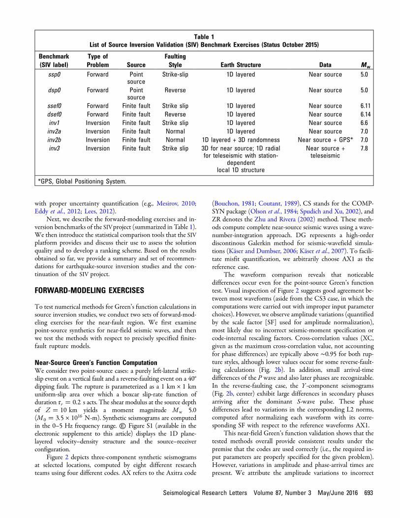
Figure 2 depicts three-component synthetic seismogramsat selected locations, computed by eight different researchteams using four different codes. AX refers to the Axitra code

(Bouchon, 1981; Coutant, 1989), CS stands for the COMP-SYN package (Olson et al., 1984; Spudich and Xu, 2002), andZR denotes the Zhu and Rivera (2002) method. These meth-ods compute complete near-source seismic waves using a wave-number-integration approach. DG represents a high-orderdiscontinous Galerkin method for seismic-wavefield simula-tions (Käser and Dumbser, 2006; Käser et al., 2007). To facili-tate misfit quantification, we arbitrarily choose AX1 as thereference case.

The waveform comparison reveals that noticeabledifferences occur even for the point-source Green’s functiontest. Visual inspection of Figure 2 suggests good agreement be-tween most waveforms (aside from the CS3 case, in which thecomputations were carried out with improper input parameterchoices). However, we observe amplitude variations (quantifiedby the scale factor [SF] used for amplitude normalization),most likely due to incorrect seismic-moment specification orcode-internal rescaling factors. Cross-correlation values (XC,given as the maximum cross-correlation value, not accountingfor phase differences) are typically above ∼0:95 for both rup-ture styles, although lower values occur for some reverse-fault-ing calculations (Fig. 2b). In addition, small arrival-timedifferences of the P wave and also later phases are recognizable.In the reverse-faulting case, the Y -component seismograms(Fig. 2b, center) exhibit large differences in secondary phasesarriving after the dominant S-wave pulse. These phasedifferences lead to variations in the corresponding L2 norms,computed after normalizing each waveform with its corre-sponding SF with respect to the reference waveforms AX1.

This near-field Green’s function validation shows that thetested methods overall provide consistent results under thepremise that the codes are used correctly (i.e., the required in-put parameters are properly specified for the given problem).However, variations in amplitude and phase-arrival times arepresent. We attribute the amplitude variations to incorrect

Table 1List of Source Inversion Validation (SIV) Benchmark Exercises (Status October 2015)

Benchmark(SIV label)

Type ofProblem Source

FaultingStyle Earth Structure Data Mw

ssp0 Forward Pointsource

Strike-slip 1D layered Near source 5.0

dsp0 Forward Pointsource

Reverse 1D layered Near source 5.0

ssef0 Forward Finite fault Strike slip 1D layered Near source 6.11dsef0 Forward Finite fault Reverse 1D layered Near source 6.14inv1 Inversion Finite fault Strike slip 1D layered Near source 6.6inv2a Inversion Finite fault Normal 1D layered Near source 7.0inv2b Inversion Finite fault Normal 1D layered + 3D randomness Near source + GPS* 7.0inv3 Inversion Finite fault Strike slip 3D for near source; 1D radial

for teleseismic with station-dependent

local 1D structure

Near source +teleseismic

7.8

*GPS, Global Positioning System.

Seismological Research Letters Volume 87, Number 3 May/June 2016 693

▴ Figure 2. (a) Three-component waveform comparison at site 10 (Ⓔ Fig. S1b) for the strike-slip point-source forward-modeling case.(b) Same as (a) for the dip-slip case at site 2 (Ⓔ Fig. S1c). Wave amplitudes are normalized by the indicated scale factor (SF) before computingthe L2 norm (L2). Cross-correlation values (XC), scale factor, and L2 norm are calculated with respect to the selected reference (AX1; peakamplitude [in m=s] given in top left). Waveforms are aligned to hypocentral time, t � 0. We observe an overall good visual agreement, withsmall time shifts but occasionally large-amplitude variations. Calculation CS3 used an incorrect input parameterization for the forward solver.

694 Seismological Research Letters Volume 87, Number 3 May/June 2016

code parameterization or incorrect use of units, whereas phase-arrival differences of a few samples are due to the particularimplementation of the source time function. When filteringthese synthetics to the frequency range typically used in sourceinversions (0–1 Hz), these timing issues become insignificant.

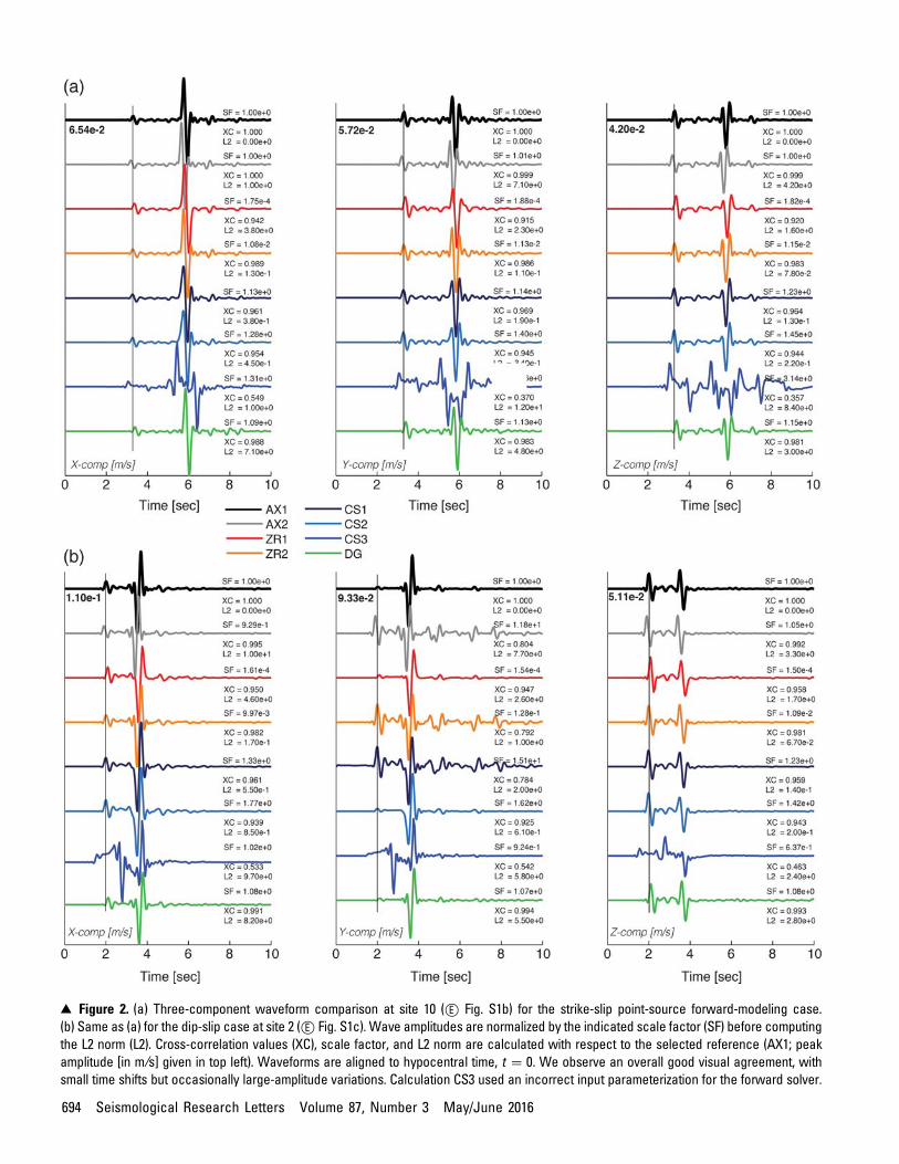
Near-Source Extended-Fault CalculationsNext, we consider two forward-modeling exercises for extended-fault ruptures that are specified in terms of 2D arrays of slip, risetime, and rupture-onset time over a planar fault surface. Thestrike-slip rupture occurs on a 12-km-long by 11-km-wide ver-tical fault, with seismic moment M0 � 1:66 × 1018 N·m(Mw � 6:11) and hypocentral depth Z � 14 km. Slip and risetime are heterogeneous over the fault, the rupture-onset times ateach point reflect variable rupture speed. The slip-rate functionon each point of the fault is a boxcar. The thrust-faulting case issimilar in dimension (12 km × 12 km fault plane) and magni-tude (M0 � 1:82 × 1018 N·m, Mw � 6:14) and in kinematicrupture characteristics, but dips at an angle of 40°. Figure 3 dis-plays the geometry and final slip on the fault for both cases.Station geometry and velocity–density structure are chosenidentical to the point-source exercise (Ⓔ Fig. S1).

Similar to the point-source forward-modeling exercise, weobserve differences in the provided solutions (Fig. 4), relatedmostly to variations in amplitude and frequency content. Forthe strike-slip case, waveforms agree well with each other, withcross-correlation coefficients typically above 0.88 (Fig. 4c). Pro-nounced differences in phase-arrival times are detectable in thedip-slip case for solution 5 (Fig. 4d), but for the other solutionsamplitude variations of different wave packets result in cross-correlation coefficients typically above 0.9 that increase to val-ues ∼0:95 after low-pass filtering (Fig. 4e). The flexible and fastonline calculation and display of the root mean square (rms)misfit and cross-correlation-coefficient matrices (Fig. 4b–e)

help to visually and quantitatively appreciate the differencesbetween the individual solutions.

Lessons Learned From Extended-Fault Forward-ModelingTestsThe SIV forward-modeling exercises for near-source seismo-grams due to point-source and extended-fault ruptures revealthat the tested codes provide overall consistent results. How-ever, we detect small phase-arrival time variations (for the pointsource) and significant amplitude differences (for both cases).Interestingly, in each case one forward-modeling solution is ob-viously incorrect, most likely due to a false input parameter-ization for the particular code used in that simulation.

Subtle variations in amplitude and phase-arrival times forthe generally consistent solutions highlight the necessity thatsource inversion scientists be intimately familiar with the for-ward-modeling codes. Often, several code versions of the samemethod are available but may lead to slightly different results.Also, computer programs may have internal tuning parametersand/or require carefully chosen case-dependent parameter val-ues. If these are not adequately specified, inaccurate results areexpected. In addition, forward-modeling codes may not becomprehensively documented and/or researchers use themin an error-prone black-box mode. We therefore strongly ad-vise source inversion researchers to conduct careful forward-modeling tests and calibrations prior to the actual source in-version study. The SIV project provides appropriate forward-modeling exercises, as well as an online platform for analyzingthe results.

INVERSION BENCHMARKS

Three SIV inversion benchmarks have been defined so far: twofor which only near-field seismograms are disseminated and

▴ Figure 3. Fault–receiver geometry and final slip on the fault for the extended-fault forward-modeling exercises: (left) strike-slip case,and (right) reverse-faulting case. Red lines mark the surface projection of the fault, black dots indicate locations on which the kinematicsource parameters are specified, and green triangles mark the receiver locations (see also Ⓔ Fig. S1b,c).

Seismological Research Letters Volume 87, Number 3 May/June 2016 695

one for which teleseismic or GPS synthetics are also provided.A fourth benchmark is under development. All benchmarkshave different characteristics and are summarized below.

The corresponding results and detailed statistical evaluationof the inversion solutions are described in the Statistical Analy-sis section.

▴ Figure 4. Three-component waveform comparisons for the extended-fault forward-modeling exercises at selected stations (ⒺFig. S1b). (a) Strike-slip case (slip model show in Fig. 3a) with six different modeling solutions at three sites. (b) Example for the rootmean square (rms) misfit matrix for three-component waveforms at a single station. (c) Example for the cross-correlation coefficientmatrix for three waveform components. (d) Dip-slip case (slip model shown in Fig. 3b) with horizontal waveforms at three locationsand corresponding cross-correlation matrices. Notice the time shifts and high-frequency oscillations in solution 5. (e) Same as (d) afterremoving solution 5 from the analysis and low-pass filtering at 1 Hz. (Continued)

696 Seismological Research Letters Volume 87, Number 3 May/June 2016

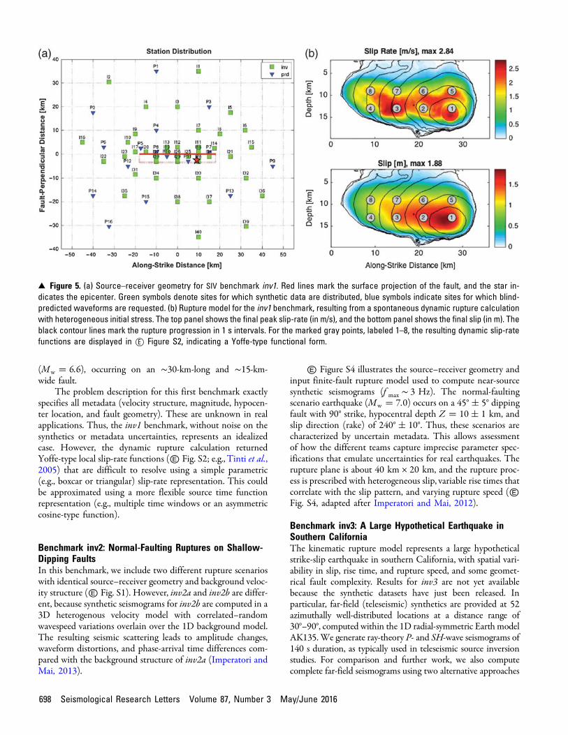
Benchmark inv1: A Strike-Slip Rupture on an 80°Dipping FaultThe first inversion benchmark, inv1, is based on a spontaneousdynamic rupture simulation for a strike-slip fault on an 80° dip-ping fault plane. The initial stress conditions were chosen usingheterogeneous initial shear stress, depth-dependent normalstress, and a slip-weakening length scale of Dc � 0:4 m thatincreased at the fault edges to a larger value (Dc � 2:0 m) to

ensure smooth rupture termination. The velocity–density struc-ture is identical to the one used in the forward-modeling exer-cises (Ⓔ Fig. S1). Near-fault seismograms (f max ∼ 2:5 Hz) werecomputed at 56 sites, but data were distributed for only 40 sites.The modeling teams had to blind-predict the seismograms at theremaining 16 locations. Figure 5 displays the fault–receivergeometry and final peak slip-rate and final slip distributions.The seismic moment of the event is M0 � 1:06 × 1019 N·m

Figure 4. Continued.

Seismological Research Letters Volume 87, Number 3 May/June 2016 697

(Mw � 6:6), occurring on an ∼30-km-long and ∼15-km-wide fault.

The problem description for this first benchmark exactlyspecifies all metadata (velocity structure, magnitude, hypocen-ter location, and fault geometry). These are unknown in realapplications. Thus, the inv1 benchmark, without noise on thesynthetics or metadata uncertainties, represents an idealizedcase. However, the dynamic rupture calculation returnedYoffe-type local slip-rate functions (Ⓔ Fig. S2; e.g., Tinti et al.,2005) that are difficult to resolve using a simple parametric(e.g., boxcar or triangular) slip-rate representation. This couldbe approximated using a more flexible source time functionrepresentation (e.g., multiple time windows or an asymmetriccosine-type function).

Benchmark inv2: Normal-Faulting Ruptures on Shallow-Dipping FaultsIn this benchmark, we include two different rupture scenarioswith identical source–receiver geometry and background veloc-ity structure (Ⓔ Fig. S1). However, inv2a and inv2b are differ-ent, because synthetic seismograms for inv2b are computed in a3D heterogenous velocity model with correlated–randomwavespeed variations overlain over the 1D background model.The resulting seismic scattering leads to amplitude changes,waveform distortions, and phase-arrival time differences com-pared with the background structure of inv2a (Imperatori andMai, 2013).

Ⓔ Figure S4 illustrates the source–receiver geometry andinput finite-fault rupture model used to compute near-sourcesynthetic seismograms (f max ∼ 3 Hz). The normal-faultingscenario earthquake (Mw � 7:0) occurs on a 45°� 5° dippingfault with 90° strike, hypocentral depth Z � 10� 1 km, andslip direction (rake) of 240°� 10°. Thus, these scenarios arecharacterized by uncertain metadata. This allows assessmentof how the different teams capture imprecise parameter spec-ifications that emulate uncertainties for real earthquakes. Therupture plane is about 40 km × 20 km, and the rupture proc-ess is prescribed with heterogeneous slip, variable rise times thatcorrelate with the slip pattern, and varying rupture speed (ⒺFig. S4, adapted after Imperatori and Mai, 2012).

Benchmark inv3: A Large Hypothetical Earthquake inSouthern CaliforniaThe kinematic rupture model represents a large hypotheticalstrike-slip earthquake in southern California, with spatial vari-ability in slip, rise time, and rupture speed, and some geomet-rical fault complexity. Results for inv3 are not yet availablebecause the synthetic datasets have just been released. Inparticular, far-field (teleseismic) synthetics are provided at 52azimuthally well-distributed locations at a distance range of30°–90°, computed within the 1D radial-symmetric Earth modelAK135.We generate ray-theory P- and SH-wave seismograms of140 s duration, as typically used in teleseismic source inversionstudies. For comparison and further work, we also computecomplete far-field seismograms using two alternative approaches

▴ Figure 5. (a) Source–receiver geometry for SIV benchmark inv1. Red lines mark the surface projection of the fault, and the star in-dicates the epicenter. Green symbols denote sites for which synthetic data are distributed, blue symbols indicate sites for which blind-predicted waveforms are requested. (b) Rupture model for the inv1 benchmark, resulting from a spontaneous dynamic rupture calculationwith heterogeneous initial stress. The top panel shows the final peak slip-rate (in m/s), and the bottom panel shows the final slip (in m). Theblack contour lines mark the rupture progression in 1 s intervals. For the marked gray points, labeled 1–8, the resulting dynamic slip-ratefunctions are displayed in Ⓔ Figure S2, indicating a Yoffe-type functional form.

698 Seismological Research Letters Volume 87, Number 3 May/June 2016

(Kikuchi and Kanamori, 1991; Friederich and Dalkolmo, 1995;Nissen-Meyer et al., 2014; van Driel et al., 2015). Figure 6 showsexample waveforms and the station distribution for the inv3-teleseismic synthetic data.

Near-source strong-motion synthetics are computed in a3D Earth model of southern California (SCEC CVM4;

Kohler et al., 2003) with a generalized finite-difference method(Ely et al., 2008). The near-surface velocity structure is trun-cated to a minimum shear wavespeed of 620 m=s, thereforef max ∼ 1 Hz. Near-field synthetics are provided for a dense sta-tion network with an interstation spacing on the order of20 km. Figure 7 depicts the near-source receiver geometry

▴ Figure 6. Example of teleseismic waveforms for inversion benchmark inv3 at four stations. The red star marks the epicenter. SHwaveforms are shown on the left and P-wavetrains are on the right. Synthetics are computed using the direct Green’s function method(DGFunc; Friederich and Dalkolmo, 1995), an axisymmetric spectral-element method (AXIsem; Nissen-Meyer et al., 2014; van Driel et al.,2015), and two implementations of a global ray-theory approach (RayThe1 and RayThe2; Kikuchi and Kanamori, 1991). The first twomethods provide the complete seismic wavefield for a spherically layered isotropic Earth.

Seismological Research Letters Volume 87, Number 3 May/June 2016 699

for the inv3 benchmarks and shows example near-field syn-thetics at selected stations. In this benchmark, source inversionteams may adopt the specified 3D Earth structure in their inver-sion or use an appropriately simplified velocity–density structure.The later analysis of inversion solutions and data predictions willillustrate the effects of the assumed velocity–density structure onsource-model uncertainties (e.g., Razafindrakoto and Mai, 2014;Gallovic et al., 2015).

Forthcoming BenchmarksForthcoming source inversion benchmarks are built on the expe-rience gleaned from the inv1–inv3 exercises. They will include ad-ditional intricacy, in particular in terms of 3D Earth structure(including topography) and geometrical rupture complexity. Com-puting the synthetic datasets at the required resolution such thatthey contain relevant information about the space–time ruptureevolution will require substantial computational resources, modern

high-performance computing (HPC)-architecture, and advancednumerical forward solvers.

We also plan to provide additional datasets that help to es-timate earthquake source processes. Recently, backprojection im-aging has been successfully applied to track the rupture evolutionin space and time (e.g., Ishii et al., 2005; Krüger and Ohrnberger,2005; Koper et al., 2011; Meng et al., 2011, 2012; Kiser and Ishii,2012; Fan and Shearer, 2015). However, it is still unclear howexactly the backprojected image relates to kinematic ruptureproperties (e.g., fault slip), because it utilizes primarily thehigh-frequency seismic wavefield (typically f ∼ 1 Hz). Recentwork attempts to generalize the backprojection technique andto incorporate it into linear inversions (Zhang et al., 2014). Dedi-cated benchmark exercises may help relate backprojection to fi-nite-fault inversions to more comprehensively characterize theunderlying rupture process. For future SIV benchmarks of largesubduction-earthquake scenarios, we may also provide synthetictsunami waveform data, which are used to constrain slip on the

▴ Figure 7. Map view of rupture geometry and near-fault receivers for inversion benchmark inv3. The star marks the epicenter, and the colorcoding reflects the shear-wavespeed at the Earth’s surface. Three-component synthetic seismograms at selected stations reveal effects ofdirectivity and 3D Earth structure. In each seismogram panel, we plot (from top to bottom) north–south, east–west, and the vertical componentvelocity seismogram, normalized with respect to peak absolute amplitude of all three components at that location (shown in cm=s).

700 Seismological Research Letters Volume 87, Number 3 May/June 2016

fault (e.g., Satake et al., 2013). In addition, synthetic Interfero-metric Synthetic Aperture Radar (InSAR) data may be included,because these help to constrain fault geometry, fault slip, and seis-mic moment (e.g., Jónsson et al., 2002). By providing multipledatasets for a single SIV benchmark, we will test how differentdata-weighting schemes affect the inversion solutions.

STATISTICAL ANALYSIS

Our goal is to statistically evaluate how well the SIV solutionsreproduce the synthetic data and the input rupture model. Weuse common waveform misfit measures (L1 norm, L2 norm,variance reduction, cross-correlation coefficient), as well astime–frequency envelope misfits and time-frequency phasemisfits (Kristekova et al., 2009). Quantitatively comparing2D fields of rupture parameters (e.g., slip, rupture time, risetime) requires defining adequate misfit measures. Mai et al.(2007) used the 2D cross-correlation coefficient and thepower-spectral decay of slip. For the SIV inversion solutions,we apply the spatial-prediction comparison test to the slipmodels (Zhang et al., 2015) and the multidimensional scaling(MDS) approach of Razafindrakoto et al. (2015). These meth-ods implement dissimilarity quantification between two physi-cal fields (e.g., slip models) and allow for ranking these fieldswith respect to a chosen reference. If the true model is known,one can define metrics to discriminate between “excellent” sol-utions and “good,” “fair,” or “poor” solutions (Razafindrakotoet al., 2015). For further details, we refer the reader to the cor-responding publications. Below, we describe inversion resultsand their statistical analysis for benchmark exercise inv1 andbriefly summarize the outcome of benchmark inv2a.

Statistic for Benchmark Exercise inv1Figure 8 displays a graphical comparison of four rupture-modelsolutions (Fig. 8b–e), showing slip, rupture-onset time, and risetime, with respect to the known target model (Fig. 8a). The slipmaps in Figure 8b and 8c look similar to the input model(Fig. 8a), whereas the slip maps in Figure 8d and 8e reveal dif-ferent spatial patterns. The same applies to rupture-onset timeand rise time. Remarkably, all three-component waveforms arevery similar (Ⓔ Fig. S3a), with acceptable rms misfit values (ⒺFig. S3b) and high cross-correlation coefficients (typicallyabove∼0:85;Ⓔ Fig. S3c). This illustrates that waveform misfitmeasures are not necessarily diagnostic of model error.

To further examine rupture-model similarities, the SIVplatform provides a summary table of scalar source-parametermetrics (Ⓔ Table S1) that list seismic moment, maximum slip,different source-dimension measures, and the slip centroid.Note that consistency in the macroscopic scalar source param-eters between the various models does not imply an agreementin the corresponding spatial distribution of slip. A first-orderqualitative appraisal for rupture-model similarity can begleaned from contour plots of rupture area, slip, rupture-onsettime, and rise time (Fig. 9). For benchmark inv1, the rupture-onset times agree quite well for about the first 3 s of the rupturebut start deviating subsequently.

Ranking rupture-model solutions with respect to eachother, or with respect to a known solution, requires statisticallyrobust misfit measures. Zhang et al. (2015) developed andtested several misfit measures for earthquake slip models usingthe spatial-prediction comparison test (SPCT, Hering andGenton, 2011), in which a chosen loss function quantifiesthe error between two 2D fields. Zhang et al. (2015) calibratedthe SPCTapproach by testing various loss functions (squared-error loss [SE], absolute-error loss [AE], and correlation skill[CK]) that are sensitive to different spatial correlation lengthsor different heterogeneity levels of slip. Their analysis showsthat the SPCT method provides an effective tool to quantita-tively rank slip models. Razafindrakoto et al. (2015) appliedthe above loss functions to an MDS approach to further compareand rank rupture models. Their work shows the ability of theSPCT and MDS methods to classify slip models even if a truereference solution does not exist. Applying the MDS approach to20 published rupture models for the 2011 Tohoku earthquakedemonstrates quantitatively how different data types affect thefinal slip distribution (Razafindrakoto et al., 2015).

The outcome of the MDS approach for inv1 benchmark isshown graphically (Fig. 10) and in tabulated format (ⒺTable S2)for dissimilarity values computed using the normalized SE. Basedon calibrated test results, Razafindrakoto et al. (2015) proposethat a normalized dissimilarity value <5 indicates an “excel-lent” agreement between two slip models. A “good” agreementis found if this value falls in the 5–20 interval, the 20–40 rangeindicates a “fair” agreement, and beyond the agreement is“poor.” Applying these definitions to solutions of benchmarkinv1 and choosing the known target solution as the reference, wefind that solution fsg is best, obtained using a new frequency-domain inversion approach (Fan et al., 2014), resulting inthe smallest dissimilarity value (Ⓔ Table S2). Solution gallovic2ranks second best. These two solutions are shown in Figure 8b,cfor a visual comparison of the slip patterns.

Many proposed solutions fall in the category “good,” indi-cating consistency between the inferred and known slip distri-bution (Fig. 10). In this example, the “best model” is determinedusing the selected MDS metric (SE). Choosing the AE or CKmay return a different ranking. Note that this ranking does notaccount for other rupture properties (rise time; rupture-onsettime) or waveform misfit.

Statistic for Benchmark Exercise inv2aWe encourage the reader to apply the online comparison toolsof the SIV platform to benchmark exercise inv2a. Examples aregiven in Ⓔ Figures S5 and S6, which show rupture-model sol-utions, scalar source-model parameters, and a selection of seismicwaveforms. For inv1, variations are observed in seismic momentby a factor ∼1:5 and in maximum slip by a factor ∼7. Solutionsfor inv2a appear to be more similar (factor ∼1:4 in seismic mo-ment, factor ∼4 in maximum slip). Ranking the solutions is notpossible based on these macroscopic source parameters or usingthe apparent waveform similarity (Ⓔ Fig. S6b). As for the inv1case, the inv2a benchmark demonstrates that good waveformfitting can be achieved despite remarkably different rupture

Seismological Research Letters Volume 87, Number 3 May/June 2016 701

models. Applying the MDS approach outlined above to thesesolutions, we find that only four models fall in the “good” cat-egory (Ⓔ Fig. S6c,d), but it is clear that two solutions, asano andgallovic1, clearly outperform the other solutions. An alternativeapproach to compare the complete spatial–temporal rupturepropagation by exploiting the eigenstructure of the inverse prob-lem is proposed by Gallovič and Ampuero (2015).

SUMMARY, RECOMMENDATIONS, AND FUTUREGOALS

The SIV collaboration continues its activities, gathering insighton how to optimally conduct earthquake source inversions andto properly test and quantify their resolving power. The SIVtests reveal that even the computation of synthetic seismograms

▴ Figure 8. Slip-inversion results for benchmark inv1. The input model is given in (a), inversion solutions are shown in (b)–(e) in terms offinal slip (top), rupture time (bottom left), and rise time (bottom right). The color scale for each source parameter, shown in (a), is identicalfor the five rupture models. The white star marks the hypocenter. Note that the actual fault-plane dimensions may not be identicalbecause these had to be chosen by the modeling teams.

702 Seismological Research Letters Volume 87, Number 3 May/June 2016

for a point source or precisely specified finite-fault rupture iserror prone. Although validated computer programs generallygenerate consistent results, inadvertently choosing slightly in-correct input parameters for a given code may jeopardize theforward simulations. Many codes are poorly documented (if atall), and/or hidden parameters in the code require tuning for agiven problem. However, users are often not the code authorsand may treat them as “black boxes,” without knowing aboutthe inner workings of the forward-modeling engine and its po-tential problems. Therefore, we recommend that any source-modeler verifies and tests the chosen forward-modeling codewith respect to published solutions. The SIV effort providessuch benchmark tests. We also recommend testing new slipinversion methods using the SIV benchmarks.

The inversion results for benchmarks inv1 and inv2adocument that an excellent waveform fit (quantified by smallrms misfit values) does not guarantee a good recovery of the“true” rupture model. Significantly different kinematic sourcemodels may explain the data equally well. At this point, we havenot investigated the potential influence of a chosen misfit func-tion for a particular inversion method. However, we find thatthe inversion methods proposed by Gallovic et al. (2015) andFan and Shearer (2015) perform particularly well. Common toboth methods is that these regularized linear inversions are un-

constrained in the temporal rupture evolution. The functionalform of the local on-fault slip-rate function is not prescribed,and there is no assumption on rupture speed. Instead, the rup-ture is allowed to develop in space and time as preferred by thedata, with adequately dense temporal sampling to recover thelocal slip-rate function. Given our current test results, thesetypes of methods appear as being best suited to estimate thespatiotemporal rupture evolution from near-fault data suchthat subsequent inferences can be made on the dynamic rup-ture process. However, further tests are needed to confirm thisconjecture, including, for instance, benchmarks with complexrupture geometry in 3D Earth structure. Furthermore, includ-ing backprojecting imaging into the linear inversion (Zhanget al., 2014) may provide a promising path forward. In futurebenchmarks, we plan to supply additional synthetic datasets(GPS; InSAR, tsunami data for a subduction-zone benchmark)to also test joint inversion strategies and corresponding data-weighting schemes.

We describe an approach to quantify the goodness of fit ofinverted rupture models with respect to an input model, basedon statistical analyses using the SPCT (Hering and Genton,2011; Zhang et al., 2015). This approach is extended to rankthe solutions using MDS (Razafindrakoto et al., 2015). Alter-native methods for statistical quantification of rupture-model

▴ Figure 9. Graphical overlay comparison of rupture-model solutions for inv1 shown in Figure 8. The true model is 1. The overlay contourplots show (a) the occupied fault area, (b) slip contours, (c) rupture-time contours, and (d) rise-time contours, using a common spatialsampling of 3 km × 3 km subfault size. These contour plots are generated using the visualization tool available on the SIV platform (seeData and Resources).

Seismological Research Letters Volume 87, Number 3 May/June 2016 703

(dis)similarities are given by Barrall and Harris (2015) or Gal-lovic and Ampuero (2015). Inspired by the SIV benchmarkresults, the latter study proposes to exploit the eigenstructureof the inverse problem. In the end, a combination of variousapproaches may best quantify similarities and differences inrupture models such that we can conclusively extract thestrength and limitations of the underlying method, data, orchosen parameterization for the source inversion problem.

It is also important to note that agreed-upon standards fordocumenting finite-fault earthquake rupture models are neededto facilitate statistical analysis and seismological research usingsource inversion results. Mai et al. (2016) propose a commonrupture-model format and describe the required level of detailfor documenting the inversion method, the data used, the pa-rameterization, and metadata. If such standards are adhered to,transparency and reproducibility of finite-fault inversions is en-sured, lending further credibility to earthquake source inversionstudies. For the SIV benchmarks, a more compact rupture-modelformat has been adopted for simplicity, but the long-term SIVgoal is to develop avenues for reproducible, testable, perhapseven (semi)automated finite-fault inversions. As such, we envi-

sion a prospective testing center in which various earthquake-source inversion codes run side by side on a range of test prob-lems first and then on real data, with minimal user intervention,to generate finite-fault rupture models with properly quantifieduncertainties. The SIV efforts described in this article are a firststep in this direction.

DATA AND RESOURCES

The earthquake rupture models shown in Figure 1 are takenfrom the online finite-fault earthquake source models(SRCMOD), available at http://equake‑rc.info/srcmod (last ac-cessed November 2015). All Source Inversion Validation (SIV)benchmarks and related problem descriptions, data, and meta-data, as well as plotting and analysis routines, can be accessedvia the SIV database (http://equake-rc.info/SIV/, last accessed De-cember 2015). The contour plots in Figure 9 are generated usingthe visualization tool available on the SIV platform (http://equake-rc.info/SIV/sivtools/list_solutions_for_benchmark/inv1/).Slip-heterogeneity characterizations are based on source modelsof past earthquakes, including an unpublished manuscript byK. K. S. Thingbaijam and P. M. Mai, “Evidence for truncatedexponential distribution of earthquake slip.”

ACKNOWLEDGMENTS

We thank Juerg Hauser for developing the initial Source In-version Validation (SIV) benchmark platform. Constructivecriticism by and inspiring discussion with Ralph Archuleta,Greg Beroza, Bill Ellsworth, Chen Ji, Ruth Harris, ThorneLay, Lingsen Meng, Peter Shearer, and others helped to steerthe SIV initiative. Constructive criticism by three anonymousreviewers helped to improve the manuscript. We are grateful tothe SRL editorial staff for their support and guidance. Thisresearch was supported by the Southern California EarthquakeCenter (Contribution Number 6159). Southern CaliforniaEarthquake Center (SCEC) is funded by National ScienceFoundation (NSF) Cooperative Agreement EAR-1033462and U.S. Geological Survey (USGS) Cooperative AgreementG12AC20038. F. G. was supported by the Czech ScienceFoundation project 14-04372S. This study is also funded byKing Abdullah University of Science and Technology(KAUST), Thuwal, Saudi Arabia. Earthquake-rupture simula-tions were carried out using the KAUST Supercomputing Lab-oratory (KSL), and we acknowledge support by KSL staff.

REFERENCES

Aki, K., and P. Richards (2002). Quantitative Seismology, Second Ed.,University Science Books, Sausalito, California.

Archuleta, R. J. (1984). A faulting model for the 1979 Imperial Valleyearthquake, J. Geophys. Res. 89, 4559–4586, doi: 10.1029/JB089iB06p04559.

Asano, K., T. Iwata, and K. Irikura (2005). Estimation of source ruptureprocess and strong ground motion simulation of the 2002 Denali,Alaska, earthquake, Bull. Seismol. Soc. Am. 95, 1701–1715.

▴ Figure 10. Rupture-model statistic for benchmark exerciseinv1, showing the multidimensional scaling (MDS) analysis forall inv1 solutions with respect to the target, “SIVdata” (indicatedby model 1). The classification of the solutions follows Razafin-drakoto et al. (2015). Symbols located in the center of the MDSgraph indicate an excellent fitting model (e.g., fsg, solution 3).Corresponding dissimilarity values are given in Ⓔ Table S2.

704 Seismological Research Letters Volume 87, Number 3 May/June 2016

Barall, M., and R. A. Harris (2015). Metrics for comparing dynamicearthquake rupture simulations, Seismol. Res. Lett. 86, 223–235,doi: 10.1785/0220140122.

Beresnev, I. A. (2003). Uncertainties in finite-fault slip inversions: Towhat extent to believe? (A critical review), Bull. Seismol. Soc.Am. 93, 2445–2458.

Bernauer, B., A. Fichtner, and H. Igel (2014). Reducing non-uniquenessin finite source inversion using rotational ground motions, J. Geo-phys. Res. 119, 4860–4875, doi: 10.1002/2014JB011042.

Blaser, L., F. Krüger, M. Ohrnberger, and F. Scherbaum (2010). Scalingrelations of earthquake source parameter estimates with special focuson subduction environment, Bull. Seismol. Soc. Am. 100, 2914–2926.

Bouchon, M. (1981). A simple method to calculate Green’s functions forelastic layered media, Bull. Seismol. Soc. Am. 71, 959–971.

Bouchon, M. (1997). The state of stress on some faults of the San An-dreas system as inferred from near-field strong motion data, J. Geo-phys. Res. 102, 11,731–11,744.

Bouchon, M., H. Karabulut, M.-P. Bouin, J. Schmittbuhl, M. Vallée, R.Archuleta, S. Das, F. Renard, and D. Marsan (2010). Faulting char-acteristics of supershear earthquakes, Tectonophysics 493, 244–253,doi: 10.1016/j.tecto.2010.06.011.

Bouchon, M., M. N. Toksoz, H. Karabulut, M. P. Bouin, M. Dietrich, M.Aktar, and M. Edie (2002). Space and time evolution of rupture andfaulting during the 1999 Izmit (Turkey) earthquake, Bull. Seismol.Soc. Am. 92, 256–266.

Causse, M., F. Cotton, and P. M. Mai (2010). Constraining the roughnessdegree of slip heterogeneity, J. Geophys. Res. 115, no. B05304, doi:10.1029/2009JB006747.

Causse, M., L. A. Dalguer, and P. M. Mai (2013). Variability of dynamicsource parameters inferred from kinematic models of past earth-quakes, Geophys. J. Int. 196, 1754–1769.

Coutant, O. (1989). Program of numerical simulation AXITRA, ResearchReports LGIT,Université Joseph Fourier, Grenoble, France (in French).

Custódio, S., P. Liu, and R. J. Archuleta (2005). The 2004 Mw 6.0 Park-field, California, earthquake: Inversion of near-source ground mo-tion using multiple data sets, Geophys. Res. Lett. 32, L23312, doi:10.1029/2005GL024417.

Day, S. M., G. Yu, and D. J. Wald (1998). Dynamic stress changes duringearthquake rupture, Bull. Seismol. Soc. Am. 88, 512–522

Delouis, B., D. Giardini, P. Lundgren, and J. Salichon (2002). Joint in-version of InSAR, GPS, teleseismic, and strong-motion data for thespatial and temporal distribution of earthquake slip: Application tothe 1999 Izmit mainshock, Bull. Seismol. Soc. Am. 92, 278–299.

Dettmer, J., R. Benavente, P. R. Cummins, andM. Sambridge (2014). Trans-dimensional finite-fault inversion, Geophys. J. Int. 199, 735–751.

Dreger, D. S. (1994). Empirical Green’s function study of the January 17,1994 Northridge, California earthquake, Geophys. Res. Lett. 21,2633–2636.

Dunham, E. M., and R. J. Archuleta (2004). Evidence for a supersheartransient during the 2002 Denali fault earthquake, Bull. Seismol.Soc. Am. 94, S256–S268, doi: 10.1785/0120040616.

Duputel, Z., L. Rivera, Y. Fukahata, and H. Kanamori (2012). Uncer-tainty estimations for seismic source inversions, Geophys. J. Int.190, doi: 10.1111/j.1365-246X.2012.05554.x.

Eddy, D.M.,W. Hollingworth, J. J. Caro, J. Tsevat, K. M. McDonald, andJ. B. Wong (2012). Model transparency and validation: A report ofthe ISPOR-SMDM Modeling Good Research Practices Task Force-7, Med. Decis. Making 32, 733–743.

Ely, G. P., S. M. Day, and J. B. Minster (2008). A support‐operatormethod for viscoelastic wave modelling in 3‐D heterogeneous me-dia, Geophys. J. Int. 172, no. 1, 331–344.

Fan, W., and P. M. Shearer (2015). Detailed rupture imaging of the 25April 2015 Nepal earthquake using teleseismic P waves, Geophys.Res. Lett. 42, doi: 10.1002/2015GL064587.

Fan, W., P. M. Shearer, and P. Gerstoft (2014). Kinematic earthquakerupture inversion in the frequency domain, Geophys. J. Int. 199,1138–1160.

Friederich, W., and J. Dalkolmo (1995). Complete synthetic seismo-grams for a spherical symmetric Earth by a numerical computationof the Green’s function in the frequency domain, Geophys. J. Int.122, 537–550.

Gabriel, A. A., J.-P. Ampuero, L. A. Dalguer, and P. M. Mai (2012). Thetransition of dynamic rupture modes in elastic media, J. Geophys.Res. 117, no. B9, doi: 10.1029/2012JB009468.

Gallovic, F., and J.-P. Ampuero (2015). A new strategy to compare in-verted rupture models exploiting the eigen-structure of the inverseproblem, Seismol. Res. Lett. 86, 1679–1689.

Gallovic, F.,W. Imperatori, and P. M. Mai (2015). Effects of three-dimen-sional crustal structure and smoothing constraint on earthquake slipinversions: Case study of the Mw 6.3 2009 L’Aquila earthquake,J. Geophys. Res. 120, 428–449, doi: 10.1002/2014JB011650.

Graves, R. W., and D. J. Wald (2001). Resolution analysis of finite faultsource inversion using one- and three-dimensional Green’s func-tions 1. Strong motions, J. Geophys. Res. 106, 8745–8766.

Gusev, A. A. (2011). Statistics of the values of a normalized slip inthe points of an earthquake fault, Izvestiya Phys. Solid Earth 47,176–185.

Harris, R. A., M. Barall, R. Archuleta, B. Aagaard, J.-P. Ampuero, H.Bhat, V. Cruz-Atienza, L. Dalguer, P. Dawson, S. Day, et al.(2009). The SCEC/USGS Dynamic Earthquake Rupture CodeVerification Exercise, Seismol. Res. Lett. 80, 119–126.

Hartzell, S. H., and T. H. Heaton (1983). Inversion of strong groundmotion and teleseismic waveform data for the fault rupture historyof the 1979 Imperial Valley, California, earthquake, Bull. Seismol.Soc. Am. 73, 1553–1583.

Hartzell, S., P. Liu, and C. Mendoza (1996). The 1994 Northridge,California, earthquake: Investigation of rupture velocity, risetime, andhigh-frequency radiation, J. Geophys. Res. 101, 20,091–20,108.

Hartzell, S., P. Liu, C. Mendoza, C. Ji, and K. M. Larson (2007). Sta-bility and uncertainty of finite-fault slip inversions: Application tothe 2004 Parkfield, California, earthquake, Bull. Seismol. Soc. Am.97, 1911–1934.

Hayes, G. (2011). Rapid source characterization of the 2011 Mw 9.0Off the Pacific Coast of Tohoku earthquake, Earth Planets Space63, 529–534.

Heaton, T. H. (1990). Evidence for and implications of self-healing pulsesof slip in earthquake rupture, Phys. Earth Planet. In. 64, 1–20.

Hering, A., and M. G. Genton (2011). Comparing spatial predictions,Technometrics 53, 414–425.

Ide, S. (2007). Slip inversion, in Treatise on Geophysics, in EarthquakeSeismology, H. Kanamori (Series Editor), Vol. 4, Elsevier, Amster-dam, The Netherlands, 193–224, ISBN: 978-0-444-51932-0.

Ide, S., and M. Takeo (1997). Determination of constitutive relations offault slip based on seismic waves analysis, J. Geophys. Res. 102,27,379–27,391.

Ide, S., G. C. Beroza, and J. J. Mcguire (2005). Imaging earthquake sourcecomplexity, in Seismic Earth: Array Analysis of Broadband Seismo-grams, A. Levander and G. Nolet (Editors), American GeophysicalUnion, Washington, D.C., doi: 10.1029/157GM08.

Imperatori,W., and P. M. Mai (2012). Sensitivity of broad-band ground-motion simulations to earthquake source and Earth structure var-iations: An application to the Messina Straits (Italy), Geophys. J. Int.118, 1103–1116, doi: 10.1111/j.1365-246X.2011.05296.x.

Imperatori,W., and P. M.Mai (2013). Broadband near-field ground-motionsimulations in 3D scattering media, Geophys. J. Int. 192, 725–744.

Ishii, M., P. M. Shearer, H. Houston, and J. E. Vidale (2005). Extent,duration and speed of the 2004 Sumatra–Andaman earthquake im-aged by the Hi-net array, Nature 435, 933–936.

Jónsson, S., H. Zebker, P. Segall, and F. Amelung (2002). Fault slip dis-tribution of the 1999Mw 7.1 Hector Mine, California, earthquake,estimated from satellite radar and GPS measurements, Bull. Seismol.Soc. Am. 92, 1377–1389.

Käser, M., and M. Dumbser (2006). An arbitrary high order discontinu-ous Galerkin method for elastic waves on unstructured meshes, I:

Seismological Research Letters Volume 87, Number 3 May/June 2016 705

The two-dimensional isotropic case with external source terms, Geo-phys. J. Int. 166, 855–877.

Käser, M., P. M. Mai, and M. Dumbser (2007). Accurate calculation offault rupture models using the high-order discontinuous Galerkinmethod on tetrahedral meshes, Bull. Seismol. Soc. Am. 97, 1570–1586.

Kikuchi, M., and H. Kanamori (1991). Inversion of complex body wavesIII, Bull. Seismol. Soc. Am. 81, 2335–2350.

King, G. C. P., R. S. Stein, and J. Lin (1994). Static stress changes and thetriggering of earthquakes, Bull. Seismol. Soc. Am. 84, 935–953.

Kiser, E., and M. Ishii (2012). Combining seismic arrays to image the high-frequency characteristics of large earthquakes, Geophys. J. Int. 188,1117–1128, doi: 10.1111/j.1365-246X.2011.05299.x.

Kohler, M. D., H. Magistrale, and R. W. Clayton (2003). Mantle hetero-geneities and the SCEC reference three-dimensional seismic velocitymodel version 3, Bull. Seismol. Soc. Am. 93, 757–774.

Konca, A. O., Y. Kaneko, N. Lapusta, and J. P. Avouac (2013). Kinematicinversion of physically plausible earthquake source models obtainedfrom dynamic rupture simulations, Bull. Seismol. Soc. Am. 103,2621–2644.

Koper, K. D., A. H. T. Lay, C. Ammon, and H. Kanamori (2011). Fre-quency-dependent rupture process of the 2011 Mw 9.0 Tohokuearthquake: Comparison of short-period P-wave backprojection im-ages and broadband seismic rupture models, Earth Planets Space 63,599–602.

Kristekova, M., J. Kristek, and P. Moczo (2009). Time-frequency misfitand goodness-of-fit criteria, Geophys. J. Int. 178, 813–825, doi:10.1111/j.1365-246X.2009.04177.x.

Krüger, F., and M. Ohrnberger (2005). Tracking the rupture of theMw � 9:3 Sumatra earthquake over 1150 km at teleseismic dis-tance, Nature 435, no. 7044, 937–939, doi: 10.1038/nature03696.

Lavallée, D., P. Liu, and R. J. Archuleta (2006). Stochastic model ofheterogeneity in earthquake slip spatial distributions, Geophys.J. Int. 165, 622–640.

Lee, S.-J., B.-S. Huang, M. Ando, H.-C. Chiu, and J.-H. Wang (2011).Evidence of large scale repeating slip during the 2011 Tohoku-Okiearthquake, Geophys. Res. Lett. 38, L19306, doi: 10.1029/2011GL049580.

Lees, J. M. (2012). Open and free: Software and scientific reproducibility,Seismol. Res. Lett. 83, 751–752, doi: 10.1785/0220120091.

Liu, P., and R. J. Archuleta (2004). A new nonlinear finite fault inversionwith three-dimensional Green’s functions: Application to the 1989Loma Prieta, California, earthquake, J. Geophys. Res. 109, no. B02318,doi: 10.1029/2003JB002625.

Liu, P., S. Custódio, and R. J. Archuleta (2006). Kinematic inversion ofthe 2004 Mw 6.0 Parkfield earthquake including an approximationto site effects, Bull. Seismol. Soc. Am. 96, S143–S158, doi: 10.1785/0120050826.

Mai, P. M. (2009) Ground motion: Complexity and scaling in the nearfield of earthquake ruptures, in Encyclopedia of Complexity and Sys-tems Science,W. H. K. Lee and R. Meyers (Editors), Springer, NewYork, 4435–4474, ISBN 978-0-387-30440-3.

Mai, P. M., and G. C. Beroza (2000). Source-scaling properties from fi-nite-fault rupture models, Bull. Seismol. Soc. Am. 90, 604–615.

Mai, P. M., and G. C. Beroza (2002). A spatial random-field model tocharacterize complexity in earthquake slip, J. Geophys. Res. 107, doi:10.1029/2001JB000588.

Mai, P. M., and K. K. S. Thingbaijam (2014). SRCMOD: An onlinedatabase of finite source rupture models, Seismol. Res. Lett. 85,1348–1357.

Mai, P.M., J. Burjanek, B. Delouis, G. Festa, C. Francois-Holden, D.Monelli, T. Uchide, and J. Zahradnik (2007). Earthquake sourceinversion blindtest: Initial results and further developments, EosTrans. AGU 88, no. 52, Fall Meet. Suppl., Abstract S53C-08.

Mai, P. M., P. Shearer, J.-P. Ampuero, and Th. Lay (2016). Standards fordocumenting finite-fault earthquake rupture models, Seismol. Res.Lett. 87, no. 3, doi: 10.1785/0220150204.

Mai, P. M., P. Somerville, A. Pitarka, L. Dalguer, H. Miyake, G. Beroza,S.-G. Song, and K. Irikura (2006). Fracture-energy scaling in dy-namic rupture models of past earthquakes, in Earthquakes: RadiatedEnergy and the Physics of Faulting, A. McGarr, R. Abercrombie, andH. Kanamori (Editors), Geophysical Monograph Series, Vol. 170,283–294

Mai, P. M, P. Spudich, and J. Boatwright (2005). Hypocenter locations infinite-source rupture models, Bull. Seismol. Soc. Am. 95, 965–980.

Manighetti, I., M. Campillo, C. Sammis, P.M. Mai, and G. King (2005).Evidence for self-similar, triangular slip distributions on earth-quakes: Implications for earthquake and fault mechanics, J. Geophys.Res. 110, no. B05302, doi: 10.1029/2004JB003174.

Meng, L., J.-P. Ampuero, J. Stock, Z. Duputel, Y. Luo, and V. C. Tsai(2012). Earthquake in a maze: Compressional rupture branchingduring the 2012 Mw 8.6 Sumatra earthquake, Science 337, 724–726, doi: 10.1126/science.1224030.

Meng, L., A. Inbal, and J.-P. Ampuero (2011). A window into the com-plexity of the dynamic rupture of the 2011 Mw 9 Tohoku-Okiearthquake, Geophys. Res. Lett. 38, doi: 10.1029/2011GL048118.

Mesirov, J. P. (2010). Accessible reproducible research, Science 327, 415–416, doi: 10.1126/science.1179653.

Minson, S. E., M. Simons, and J. L. Beck (2013). Bayesian inversion forfinite fault earthquake source models I—Theory and algorithm,Geophys. J. Int. 194, 1701–1726.

Monelli, D., and P. M. Mai (2008). Bayesian inference of kinematicearthquake rupture parameters through fitting of strong motiondata, Geophys. J. Int. 173, 220–232, doi: 10.1111/j.1365-246X.2008.03733.x.

Monelli, D., P. M. Mai, S. Jónsson, and D. Giardini (2009). Bayesianimaging of the 2000 Western Tottori (Japan) earthquake throughfitting of strong motion and GPS data, Geophys. J. Int. 176, 135–150, doi: 10.1111/j.1365-246X.2008.03943.x.

Nissen-Meyer, T., M. van Driel, S. C. Stähler, K. Hosseini, S. Hempel, L.Auer, A. Colombi, and A. Fournier (2014). AxiSEM: Broadband 3-D seismic wavefields in axisymmetric media, Solid Earth 5, 425–445, doi: 10.5194/se-5-425-2014.

Olson, A. H., and R. J. Apsel (1982). Finite faults and inverse theory withapplications to the 1979 Imperial Valley earthquake, Bull. Seismol.Soc. Am. 72, 1969–2001.

Olson, A. H., J. A. Orcutt, and G. A. Frazier (1984). The discrete wave-number/finite element method for synthetic seismograms, Geophys.J. Roy. Astron. Soc. 77, 421–460.

Page, M. T., E. M. Dunham, and J. Carlson (2005). Distinguishing bar-riers and asperities in near-source ground motion, J. Geophys. Res.no. B11302, doi: 10.1029/2005JB003736.

Page, M., P. M. Mai, and D. Schorlemmer (2011). Testing earthquakesource inversion methodologies, Eos Trans. AGU 92, no. 9, 75.

Razafindrakoto, H. N. T., and P. M. Mai (2014). Uncertainty in earth-quake source imaging due to variations in source time functionand Earth structure, Bull. Seismol. Soc. Am. 104, 855–874, doi:10.1785/0120130195.

Razafindrakoto, H. N. T, P. M. Mai, M. G. Genton, L. Zhang, and K.K. S. Thingbaijam (2015). Quantifying variability in earthquakerupture models using multidimensional scaling: Application tothe 2011 Tohoku earthquake, Geophys. J. Int. 202, 17–40, doi:10.1093/gji/ggv088.

Satake, K.,Y. Fujii, T. Harada, and Y. Namegaya (2013). Time and spacedistribution of coseismic slip of the 2011 Tohoku earthquake asinferred from tsunami waveform data, Bull. Seismol. Soc. Am. 103,1473–1492.

Sekiguchi, H., and T. Iwata (2002). Rupture process of the 1999 Kocaeli,Turkey, earthquake estimated from strong-motion waveforms, Bull.Seismol. Soc. Am. 92, 300–311.

Somerville, P., K. Irikura, R. Graves, S. Sawada, D. Wald, N. Abrahamson,Y. Iwasaki, T. Kagawa, N. Smith, and A. Kowada (1999) Character-izing crustal earthquake slip models for the prediction of strongground motion, Seismol. Res. Lett. 70, 59–80.

706 Seismological Research Letters Volume 87, Number 3 May/June 2016

Spudich, P., and L. Xu (2002). Documentation of Software PackageCompsyn sxv3.11: Programs for Earthquake Ground Motion Cal-culation Using Complete 1-D Green’s Functions, InternationalHandbook of Earthquake and Engineering Seismology, AcademicPress, London.

Stein, R. S., A. A. Barka, and J. H. Dieterich (1997). Progressive failure onthe North Anatolian fault since 1939 by earthquake stress trigger-ing, Geophys. J. Int. 128, 594–604.

Strasser, F. O., M. C. Arango, and J. J. Bommer (2010). Scaling of thesource dimensions of interface and intraslab subduction-zoneearthquakes with moment magnitude, Seismol. Res. Lett. 81,941–950.

Tinti, E., P. Spudich, and M. Cocco (2005). Earthquake fracture energiesinferred from kinematic rupture models on extended faults, J. Geo-phys. Res. 110, no. B12303, doi: 10.1029/2005JB003644.

van Driel, M., L. Krischer, S. C. Stähler, K. Hosseini, and T. Nissen-Meyer (2015). Instaseis: Instant global seismograms based on abroadband waveform database, Solid Earth 6, 701–717, doi:10.5194/se-6-701-2015.

Wald, D. J., and R. W. Graves (2001). Resolution analysis of finite faultsource inversion using one-and three-dimensional Green’s func-tions: 2. Combining seismic and geodetic data, J. Geophys. Res.106, 8767–8788.

Wald, D. J., D. V. Helmberger, and T. H. Heaton (1991). Rupture modelof the 1989 Loma Prieta earthquake from the inversion of strong-motion and broadband teleseismic data, Bull. Seismol. Soc. Am. 81,1540–1572.

Yagi, Y., and M. Kikuchi (2000). Source rupture process of the Kocaeli,Turkey, earthquake of August 17, 1999, obtained by joint inversionof near-field data and teleseismic data, Geophys. Res. Lett. 27, 1969–1972.

Yoshida, S., K. Koketsu, B. Shibazaki, T. Sagiya, T. Kato, and Y. Yoshida(1996). Joint inversion of near- and far-field waveform and geodeticdata for the rupture process of the 1995 Kobe earthquake, J. Phys.Earth 44, no. 5, 437–454.

Yue, H,T. Lay, and K. D. Koper (2012). En echelon and orthogonal faultruptures of the 11 April 2012 Great Intraplate earthquakes, Nature490, 245–249, doi: 10.1038/nature11492.

Zechar, J. D., D. Schorlemmer, M. Liukis, J. Yu, F. Euchner, P. J.Maechling, and T. H. Jordan (2010). The Collaboratory forthe Study of Earthquake Predictability perspective on computa-tional earthquake science, Concurrency Comput. Pract. Ex. 22,1836–1847.

Zhang, L., P. M. Mai, K. K. S. Thingbaijam, H. N. Razafindrakoto, andM. Genton (2015). Comparing earthquake slip models with the spa-tial prediction comparison test, Geophys. J. Int. 200, 185–198, doi:10.1093/gji/ggu383.

Zhang, Y., R. Wang, J. Zschau, Y. T. Chen, S. Parolai, and T. Dahm(2014). Automatic imaging of earthquake rupture processes by iter-ative deconvolution and stacking of high-rate GPS and strong mo-tion seismograms, J. Geophys. Res. 119, 5633–5650.

Zhu, L., and L. A. Rivera (2002). A note on the dynamic and static dis-placements from a point source in multilayered media, Geophys.J. Int. 148, 619–627.

P. Martin MaiMartin Galis

Walter Imperatori1

Luca PassoneHoby N. T. Razafindrakoto2

Kiran K. S. ThingbaijamJagdish C. Vyas

Olaf ZielkeKing Abdullah University of Science and Technology

Division of Physical Sciences and Engineering

Thuwal 23955-6900, Kingdom of Saudi Arabiamartin.mai@kaust.edu.sa

Danijel SchorlemmerRongjiang Wang

Geo-Forschungszentrum Potsdam, GFZTelegrafenberg

14473 Potsdam, Germany

Morgan PageU.S. Geological Survey

525 South Wilson AvenuePasadena, California 91106 U.S.A.

Jean-Paul AmpueroCalifornia Institute of Technology

Seismological Laboratory1200 East California Boulevard

MC 252-21Pasadena, California 91125 U.S.A.

Kimiyuki AsanoHaruko Sekiguchi

Disaster Prevention Research InstituteKyoto University

Gokasho, UjiKyoto 611-0011, Japan

Mathieu CausseISTerre

Universite Grenoble Alpes, IFSTTAR, CNRSCS 40700

38058 GrenobleCedex 9, France

Susana CustodioInstituto Dom Luiz

Faculdade de CiènciasUniversidade de Lisboa

1749-016 Lisboa, Portugal

Wenyuan FanUniversity of California, San DiegoScripps Institution of Oceanography

IGPP 0225La Jolla, California 92093-0225 U.S.A.

Gaetano FestaDepartment of Physics

Università di Napoli Federico IINaples, Italy

Frantisek GallovicCharles University in Prague

Faculty of Mathematics and PhysicsDepartment of Geophysics

Seismological Research Letters Volume 87, Number 3 May/June 2016 707

V Holešovičkách 2180 00 Praha 8Czech Republic

Martin KäserDepartment of Earth and Environmental Sciences

Ludwig-Maximilian UniversityTheresienstr. 41

80333 Munich, Germany

Dmytro MalytskyyCarpathian Branch of Subbotin Institute of Geophysics

National Academy of Sciences of UkraineLviv 79060 Ukraine

Ryo OkuwakiYuji Yagi

Faculty of Life and Environmental SciencesUniversity of Tsukuba

1-1-1 Tennodai, TsukubaIbaraki 305-8572, Japan

Fred PollitzEarthquake Science Center

U.S. Geological Survey345 Middlefield Rd., MS 977

Menlo Park, California 94025 U.S.A.

Seok Goo SongEarthquake Research Center

Korea Institute of Geoscience and Mineral Resources (KI-GAM)

124 Gwahang-no, Yuseong-guDaejeon 34132, South Korea

Surendra N. SomalaDepartment of Civil Engineering

Indian Institute of Technology (IIT) HyderabadHyderabad, India 502285

Cedric TwardzikDepartment of Earth Science

1006 Webb HallUniversity of California, Santa Barbara

Santa Barbara, California 93106-9630 U.S.A.

Martin van DrielDepartment of Earth Sciences, ETH Zürich

Sonneggstrasse 58092 Zurich, Switzerland

Published Online 6 April 2016

1 Also at Department of Earth Sciences, ETH Zürich, Sonneggstrasse 5,8092 Zurich, Switzerland.2 Also at Department of Civil and Natural Resources Engineering, Uni-versity of Canterbury, Christchurch 8040, New Zealand.

708 Seismological Research Letters Volume 87, Number 3 May/June 2016