Numerical Study of Hydrodynamic Characteristics of Gas–Liquid Slug Flow in Vertical Pipe August 2016 Enass Massoud • PhD Student: Department of Naval Architecture, Ocean and Marine Engineering (NAOME), University of Strathclyde, Glasgow, United Kingdom. • Teaching Assistant: Mechanical Engineering Department, Arab Academy for Science, Technology & Maritime Transport (AASTMT), Alexandria, Egypt. • [email protected]Proceeding of Global Summit and Expo on Fluid Dynamics & Aerodynamics
Transcript
Numerical Study of Hydrodynamic Characteristics of Gas–Liquid Slug
Flow in Vertical Pipe
August 2016
Enass Massoud
• PhD Student:Department of Naval Architecture, Ocean and Marine Engineering (NAOME), University of Strathclyde, Glasgow, United Kingdom.
• Teaching Assistant:Mechanical Engineering Department, Arab Academy for Science, Technology & Maritime Transport (AASTMT), Alexandria, Egypt.
Proceeding of Global Summit and Expo onFluid Dynamics & Aerodynamics
Presentation Overview
2
1. Introduction.
2. Aim of the study.
3. Model development;
a) Governing equations.
b) Model geometry and boundary conditions.
c) Solution strategy and convergence criterion.
4. Results and discussions;
a) Taylor bubble shape.
b) Taylor bubble rise velocity.
c) Liquid film.
d) Wake flow structure.
e) Wall shear stress distribution.
5. Conclusions.
6. Recommendations for future work.
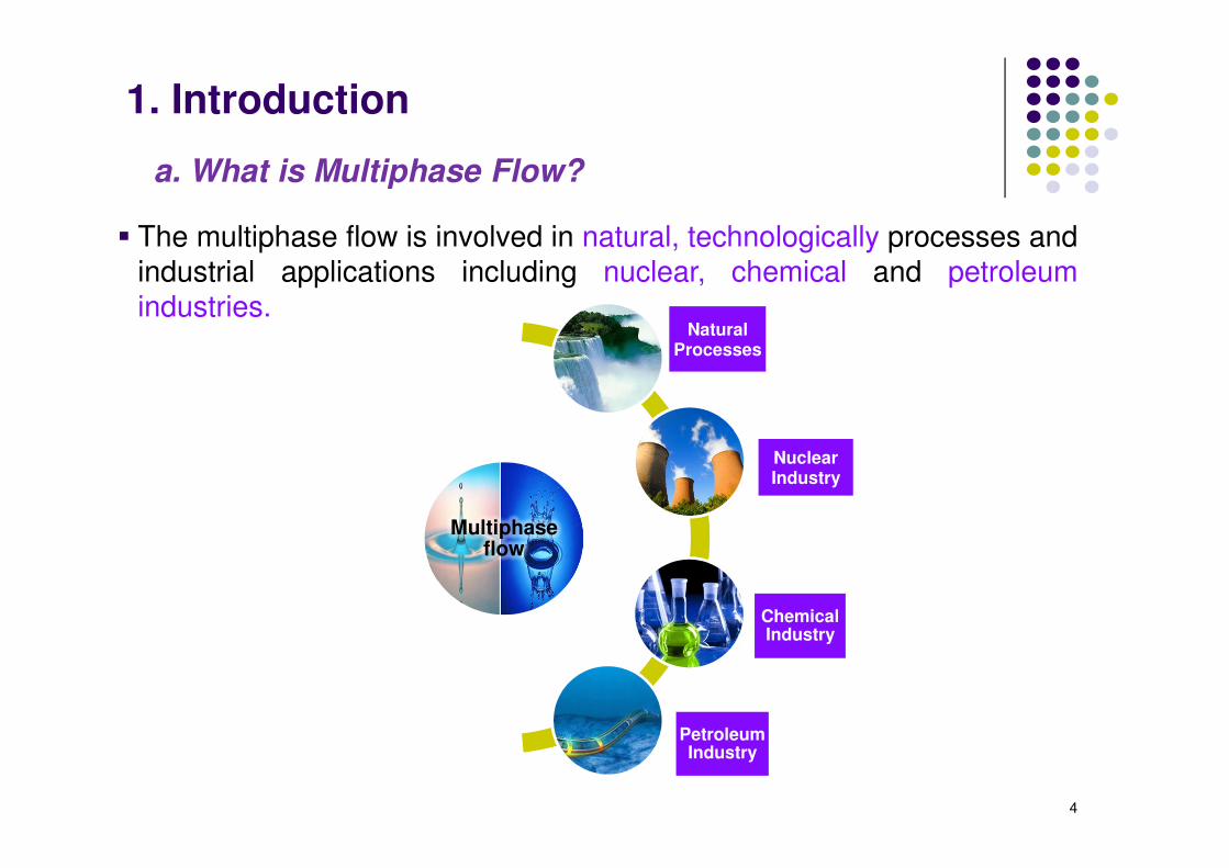
a. What is Multiphase Flow?
3
� A multiphase flow is defined as any fluid system in which there isinteraction between two or more phases (gas, solid and liquid) where theinterface between the phases is influenced by their motion.
� The multiphase flow is involved in natural, technologically processes andindustrial applications including nuclear, chemical and petroleumindustries.
Multiphase flow
Natural Processes
Nuclear Industry
Chemical Industry
Petroleum Industry
a. What is Multiphase Flow?
1. Introduction
5
� Multiphase flow can be classified according to;
b. Classifications of Multiphase Flow?
1. Introduction
Classification of Multiphase flow
Combination of the phases
Two phase flow
Three phase flow
Four phase flow
Structure of the interface (flow regime or flow pattern)
Dispersed bubbly flow
Intermitted flow
Annular flow
6
b. Classifications of Multiphase Flow?
1. Introduction
1) Two Phase Flow
Gas-liquid flows:
� It is found widely in a whole range of industrial applications;
� Pipeline systems for the transport of oil-gas mixtures,
transportation, oil processing and nuclear waste management.
7
b. Classifications of Multiphase Flow?
1. Introduction
1) Two Phase Flow
Gas-solid flows:
� Flows of solids suspended in gases are important in;
� Pulverized fuel combustion,
� Fluidized beds.
2) Three Phase Flow
Gas-liquid-liquid flows:
� Gas-oil-water flows in oil recovery systems.
Gas-liquid-solid flows:
� Two Phase Fluidized bed.
Solid-liquid-liquid flows:
� Presence of sand or solid particles in oil-water mixtures in pipelines.
8
b. Classifications of Multiphase Flow?
1. Introduction
3) Four Phase Flow
� The three phase flow is often encountered as a mixture of gas, oil and water.
� The presence of sand or other particle may result into four phase flow (G-L-L-S).
9
Gas-Liquid flow regimes in vertical pipes
Sketches of flow regimes for two-phase flow in a vertical pipe
b. Classifications of Multiphase Flow?
1. Introduction
Weisman (1983)
Mandal et al. (2010) 10
� A slug unit cell (fundamental unit)consists of an elongated bullet shapedbubbles that fills almost the entirepipeline cross section, known as TaylorBubble, a liquid film flowing downwardsbetween the bubble interface and pipewall, known as liquid slug.
� The body of the slug is liquid. But incases of high gas flow rates, somegases diffuse into the liquid slug and isreferred to as Aerated Slug.
c. Slug Flow
1. Introduction
11
� Severe slugging may appear for low gas and liquid flow rates when asection with downward inclination angle (pipeline) is followed byanother section with an upward inclination (riser). This configuration iscommon in offshore petroleum production systems.
c. Slug Flow
1. Introduction
Malekzadeh, R. (2012)
12
� According to Xing et al. (2014), the liquid slugs generated in the Oil andGas multiphase flowlines can be classified based on their initiationmechanism into;
c. Slug Flow
1. Introduction
At early and late stages of production
Terrain-induced slugs
At middle stages of production
Hydrodynamic slugs
At start up and regular pigging
operation
Operation induced slugs
13
Effects
Higher pressure drop for flow
Could cause platform trips and plant shutdown
Reduces capacity of separation and
compression units
Enhance corrosion, erosion
and fatigue in pipelines
CausesHydrodynamic
SluggingTerrain-Induced
SluggingRiser-Based
SluggingOperation-
Induced Slugging
c. Slug Flow
1. Introduction
http://petronet-
resources.co.uk.websitebu
ilder.prositehosting.co.uk/
ascomp
https://www.software.sl
b.com/products/olga/ol
ga-pipeline-
management/slug-
tracking
Mokhatab, S., & Towler, B. F.
(2007).
http://www.pipelinebundle.co
m/ser_pigging.htm
14
v. Slug flow problems-Why model slug flow?
� Flooding of downstream processing facilities.
� Reservoir flow oscillations and poor management.
� Severe pipe corrosion and structural instability of pipeline.
� The slug induces unsteady loading on pipeline and also on the receivingdevices, such as separators. This causes design problems and hencelower the system efficiency and size.
� Instabilities in liquid control system of separators due to high sudden flowrates which may lead to complete shut down.
� Production loss due to the slug induced high average back pressure.
5. Slug Flow in Subsea Oil & Gas Production System
Presentation Overview
15
1. Introduction.
2. Aim of the study.
3. Model development;
a) Governing equations.
b) Model geometry and boundary conditions.
c) Solution strategy and convergence criterion.
4. Results and discussions;
a) Taylor bubble shape.
b) Taylor bubble rise velocity.
c) Liquid film.
d) Wake flow structure.
e) Wall shear stress distribution.
5. Conclusions.
6. Recommendations for future work.
16
2. Aim of the study
� The hydrodynamic characteristics of gas-liquid vertical slug flowis governed by three main forces, namely; viscous, inertial, andinterfacial forces.
� A dimensionless analysis for two-phase gas-liquid slug flow canbe done by applying Pi-Buckingham theorem.
�� � �� ∗ � ∗ � ⁄� Eötvös number: the ratio between
gravitational forces, and surface tensionforces.
� Froude number: the ratio between the
inertia and gravitational forces ��� � ��� � ∗ �⁄� Inverse viscosity number: the ratio
� The main aim of the present investigation isto study the hydrodynamics characteristicsof single Taylor bubble rising in a stagnantNewtonian liquid using the volume-of-fluid(VOF) methodology implemented in thecomputational dynamic software package,ANSYS Fluent (Release 15.0).
� The results accounts for; Taylor bubbleshape, Taylor bubble rise velocity (��� ),liquid film (���, δ��), wake flow structure,and wall shear stress distribution (τ").
� The simulation has been performed for 2D,unsteady, laminar flow with constant fluidproperties.
� The two phases were assumed asincompressible, viscous, immiscible, andnot penetrating each other.
Presentation Overview
18
1. Introduction.
2. Aim of the study
3. Model development;
a) Governing equations.
b) Model geometry and boundary conditions.
c) Solution strategy and convergence criterion.
4. Results and discussions;
a) Taylor bubble shape.
b) Taylor bubble rise velocity.
c) Liquid film.
d) Wake flow structure.
e) Wall shear stress distribution.
5. Conclusions.
6. Recommendations for future work.
19
3. Model Development
a. Governing Equations
� The simulation domain is a vertical pipeof diameter, �, and length, #.
� The flow consists of single Taylor bubblerising in stagnant fluid.
� The volume-of-fluid (VOF) method isused to track/capture the sharp interfacesbetween two immiscible fluids (freesurface flow).
� This model solves a single set of NaiverStokes equations (NSE) that is shared bythe two fluids, and the volume fraction ofeach of the fluids in each computationalcell throughout the domain.
20
1. Reynolds Average Continuity Equation
$%$& + (. �%�� � )*+,+-.
� �: volume-fraction-averaged density
� � : time average velocity which is computed by solving the momentum
equation for the mixture (not individual components).
� / : number of the phases (for the present two phase flow, /=2).� *+ : mass source (set to zero in the present case)
3. Model Development
a. Governing Equations
2. Reynolds Average Momentum Equation$�%��$& + (. %�� � �(0 + (. 1 (� + (�� + %� + � P: pressure in the domain,
� µ : volume-fraction-averaged viscosity of the flowing fluid,
� g : acceleration due to gravity,
� F : body force.
21
� The VOF formulation relies on the fact that two or more fluids (orphases) are not interpenetrating. For each additional phase that you addto your model, a variable is introduced which is the volume fraction ofthe phase in the computational cell. In each control volume, the volumefractions of all phases sum to unity.
)2+,+-. � 1 2� + 2� � 1
3. Model Development
A. Governing Equations
� The NSEs are thus dependent on the volume fractions of all phasesthrough the volume-fraction-averaged properties; � and �.
% � )�+,+-. 2+ � 2��� + 2��� � 2��� + �1 � 2����
1 � )�+2+ � 2��� + 2��� � 2��� + �1 � 2����,+-.
22
3. Model Development
a. Governing Equations
� Tracking the interface between the two phases is achieved by thetreatment of the volume fraction of the 456 fluid, 2+ through solving a
separate continuity equation, given by;
1�+ $$& 2+�+ + (. �2+�+�+7 � *8+ + )�9:+°,
:-. �9+:° <� *8+: mass source term,
� 9:+° : mass transfer from phase = to phase 4,
� 9+:° : mass transfer from phase 4 to phase =.
3. Volume fraction equation
23
3. Model Development
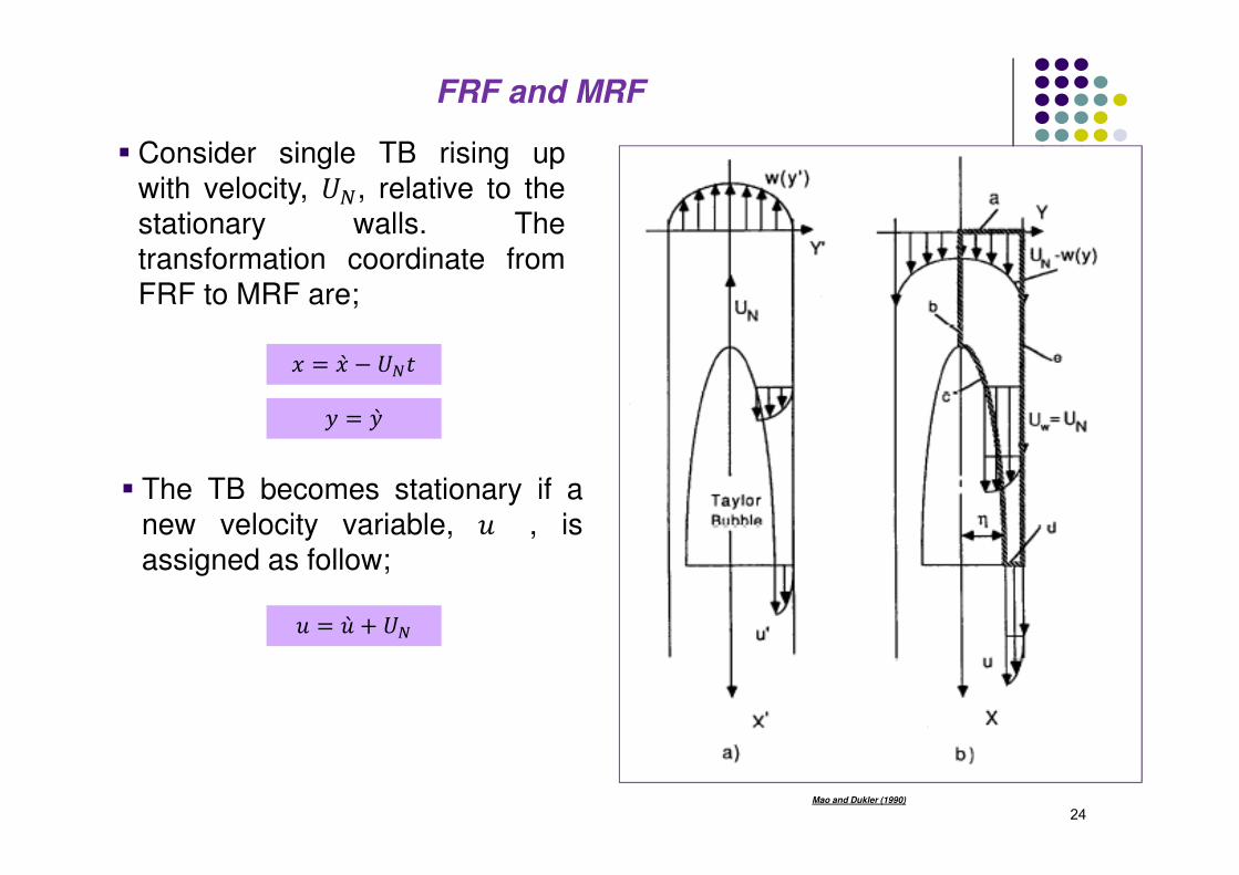
b. Model Geometry and Boundary Conditions
� The simulation is performed byattaching a reference frame to the risingTaylor bubble.
� Enabling moving reference frame(MRF) in the simulation, causes therising Taylor bubble to be stationary andthe pipe wall moves downwards withvelocity equal to that of the bubble.
� � ���� ∗ � � 0.345 1 � BC�.�.DE�.��� 1 � B�.�FCGHIwhere;9 � O25, �� R 1869��C�.��, 18 R �� R 25010, �� V 250
� The initial guess of Taylor bubble velocity, ���,is estimated according to Wallis (1969)correlation;
� The initial guess of the liquid filmthickness,W��, is estimated using Brown (1965)equation;
� Consider single TB rising upwith velocity, �D, relative to thestationary walls. Thetransformation coordinate fromFRF to MRF are;
Z � Z̀ � �D&\ � \̀� The TB becomes stationary if a
new velocity variable, ] , isassigned as follow;
] � ]̀ + �D
25
26
G-L Interface BC
� The pressure variation in the gas phase is assumed to beconstant.
� The boundary conditions at the gas-liquidinterface are given by;
]. / � 02. The dynamic boundary condition, which is
also known by stress jump condition can bedivided into two separate boundaryconditions;
a) the tangential stress balance assumingzero interfacial shear stress along theinterface; �^. /̂�. `̂ � 0
1. The kinematic condition assuming full slip atthe interface is applied;
b) the normal stress balance;
Where; ^, / ̂, `̂, , �a# and b are the shearstress, unit normal vector at the interface, unittangential vector at the interface, surfacetension, liquid phase side pressure, andcurvature of the interface, respectively.
� According to Mao and Dukler (1990),thecurvature of the interface is expressed in termsof radii of the curvature of the bubble surface,as follows;
�c� + b � d�/`&e/&
b � 1�1 + 1�2
27
3. Model Development
c. Solution Strategy and Convergence Criterion
1. Transient solver and a time step size of 0.0001s was employed.
2. The simulation was carried out using the explicit VOF model.
3. A simple scheme for the pressure-velocity coupling is considered.
4. A spatial discretization scheme used are as follows;
• Green Gauss Cell Based for Gradient.
• PRESTO for Pressure.
• Compressive for Volume fraction.
• Quick scheme for Momentum.
• First order implicit for transient formulation
5. The scaled absolute values of the residual of the calculated values ofmass, velocity in x and y directions were monitored and convergencecriterion was set to 10-3 for each time step.
6. Results were obtained using the Engineering and Physical SciencesResearch Council (EPSRC) funded ARCHIE-WeSt high performancecomputer (www.archie-west.ac.uk).
� Four cases were simulated according to the experimental workCampos and Carvalho (1988)
Velocity fields and streamlines of gas-liquid slug flow in vertical pipe of 19mm diameter, and 209 mm length,��=84, ���=0.289, and ��=66.3 using MRF
30
4. Results and Discussions
� Effect of inverse viscosity number �� on
Taylor bubble shape.
� The simulated results are in good
agreement with;
1. the experimental observations of Goldsmith
and Mason (1962); in highly viscous flow
(viscosity dominated flow) the Taylor bubble
has spheroid shape where the top end of
bubble is prolate, and the bottom end is
oblate. While, in low viscosity flow the
flattening or concaving shape of Taylor
bubble bottom end is observed.
2. the numerical work of Araújo et al. (2012),
Taha and Cui (2006), and Zheng et al.
(2007).
a. Taylor Bubble Shape
(1) kl=84, (2) kl=176, (3) kl=205, and
(4) kl=325
31
4. Results and Discussions
a. Taylor Bubble Shape
0
0.2
0.4
0.6
0.8
1
0 1 2 3 4 5 6 7
r/R
(-)
x/R (-)
Present Simulation-Nf=176
Present Simulation-Nf=84
Taha and Cui (2007)-Nf=84
Taha and Cui (2007)-NF=176
Validation of simulation results for Taylor
bubble shape profile for cases 1, and 2
with the work of Taha and Cui (2006) - mis axial distance from bubble nose.
0
0.2
0.4
0.6
0.8
1
0 1 2 3 4 5 6 7
r/R
(-)
x/R (-)
Present Simulation-Nf=176
Present Simulation-Nf=205
Present Simulation-Nf=325
Effect of no on Taylor bubble shape profile for
cases 2, 3 and 4 -m is axial distance from
bubble nose.
32
4. Results and Discussions
b. Taylor Bubble Rise Velocity, pqrCases Simulation White and Beardmore (1961) Wallis Correlation (1969)
1Case ��� 0.1251 0.1381 0.1340
Error (%) … 9.41 6.62
2Case ��� 0.1374 0.1467 0.1473
Error (%) … 6.35 6.71
3Case ��� 0.1390 0.1467 0.1480
Error (%) … 5.24 6.02
4Case ��� 0.1425 0.1424 0.1485
Error (%) … -0.07 4.0
33
4. Results and Discussions
c. Liquid Film
Effect of kl on liquid film thickness WWWWLFLFLFLF -Z is axial distance from bubble nose.
0
0.1
0.2
0.3
0.4
0.5
0.6
0 0.5 1 1.5 2 2.5 3
x/D (-)
Present Simulation-NF=84
Present Simulation-NF=176
Present Simulation-NF=205
Present Simulation-NF=325W LF/�(-
)
-0.15
-0.1
-0.05
0
0.05
0.1
0.15
0.2
0.25
0.3
0.35
0 0.5 1 1.5 2 2.5 3
ULF
(m/s
)
x/D (-)
Present Simulation-NF=84
Present Simulation-NF=176
Present Simulation-NF=205
Present Simulation-NF=325
Effect of no on liquid film axial velocity UUUULFLFLFLF - Zis axial distance from bubble nose.
34
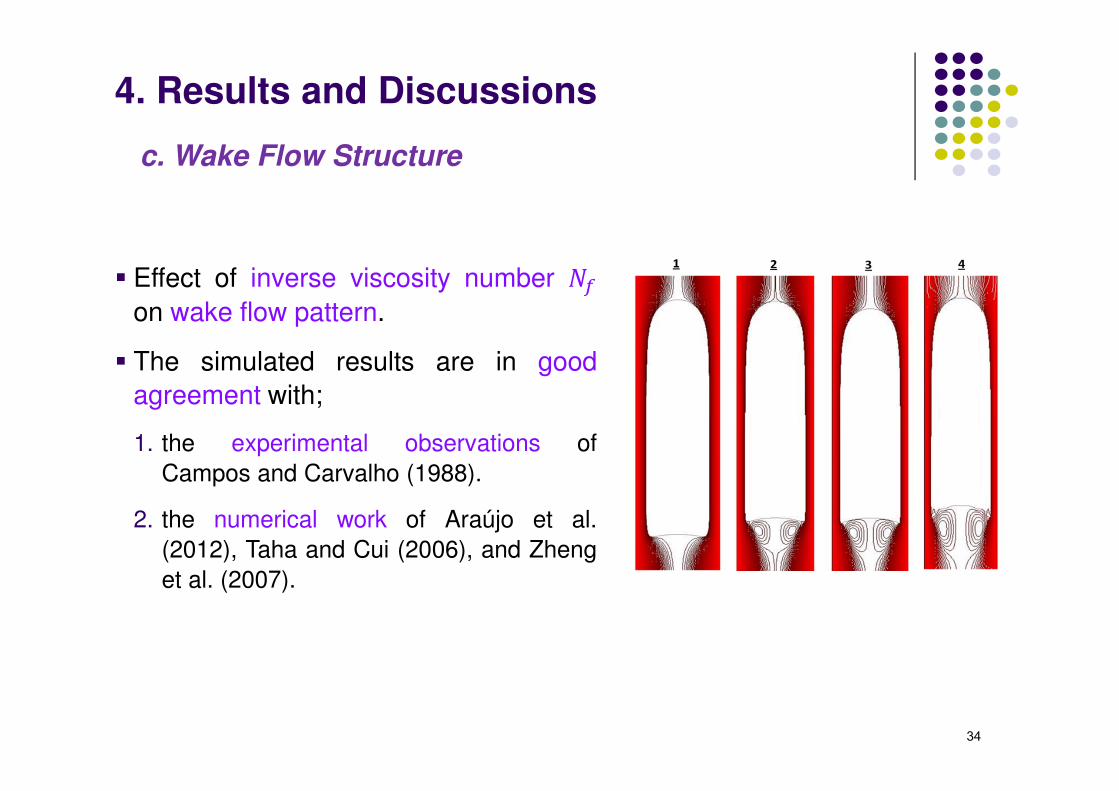
4. Results and Discussions
c. Wake Flow Structure
� Effect of inverse viscosity number ��on wake flow pattern.
� The simulated results are in good
agreement with;
1. the experimental observations of
Campos and Carvalho (1988).
2. the numerical work of Araújo et al.
(2012), Taha and Cui (2006), and Zheng
et al. (2007).
35
4. Results and Discussions
d. Wall Shear Stress Distribution
0
10
20
30
-1 0 1 2 3 4 5 6 7 8 9 10
Wa
ll s
he
ar
stre
ss (
Pa
sca
l)
x/R (-)
Present Simulation-Nf=84
Present Simulation-Nf=176
Present Simulation-Nf=205
Present Simulation-Nf=325
0
10
20
30
-1 0 1 2 3 4 5 6 7 8 9 10
Wa
ll s
he
ar
stre
ss (
Pa
sca
l)
x/R (-)
Taha and Cui (2007)-Nf=176
Taha and Cui (2007)-Nf=84
Present Simulation-Nf=84
Present Simulation-Nf=176
Validation of simulation results for the wall
shear stress distribution wx around a slug unit
with the work of Taha and Cui (2006) - m is axial
distance from bubble nose.
Effect of kl on the wall shear stress
distribution wx around a slug unit-m is axial
distance from bubble nose.
Presentation Overview
36
1. Introduction.
2. Aim of the study.
3. Model development;
a) Governing equations.
b) Model geometry and boundary conditions.
c) Solution strategy and convergence criterion.
4. Results and discussions;
a) Taylor bubble shape.
b) Taylor bubble rise velocity.
c) Liquid film.
d) Wake flow structure.
e) Wall shear stress distribution.
5. Conclusions.
6. Recommendations for future work.
37
� The following conclusions can be pointed out;
1) The Taylor bubble bottom depends on the liquid viscosity where theincrease in the inverse viscosity number,��, increases the concave shape
of the Taylor bubble bottom surface.
2) The calculated Taylor bubble rise velocity,���, is in an acceptable range
when compared with experimental values and commonly used correlations
in the literature.
3) The liquid film zone can be describes using the liquid film thickness, W��,
and the liquid film axial velocity, ��� that are both directly affected by theinverse viscosity number, ��.
4) The wake flow structure has a closed axisymmetric nature for all the
simulation cases with the development of circulatory vortex in the bubblewake with the increase in ��.
5) The wall shear stress, ^" is mainly dependent on the liquid film thickness,W��, and has a peak positive values in the stabilized liquid film zone.
4. Conclusions
Presentation Overview
38
1. Introduction.
2. Aim of the study.
3. Model development;
a) Governing equations.
b) Model geometry and boundary conditions.
c) Solution strategy and convergence criterion.
4. Results and discussions;
a) Taylor bubble shape.
b) Taylor bubble rise velocity.
c) Liquid film.
d) Wake flow structure.
e) Wall shear stress distribution.
5. Conclusions.
6. Recommendations for future work.
39
� This study set out to develop a basic simulation model for gas-liquid slugflow in vertical pipe under laminar flow regime.
� It is recommended that further research could be undertaken in thefollowing areas;
1. Investigating the hydrodynamic characteristics of slug flow fordifferent fluid system including the effect of viscosity and densityratios,
2. Investigating the hydrodynamic characteristics of slug flow underturbulent regime with��V 500,
3. Exploring the hydrodynamic characteristics of slug flow includingthe flow of two consecutive Taylor bubbles in vertical pipe,
4. Studying the wake flow pattern of single Taylor bubble or twoconsecutive Taylor bubbles under turbulent flow regime in terms ofwake volume and length.