E3 System Control Overview and Economic Dispatch...

E3 System Control Overview and Economic Dispatch Calculation 205

All materials are under copyright of PowerLearn. Copyright © 2000, all rights reserved

Module E3 Economic Dispatch Calculation

Primary Author: Gerald B. Sheble, Iowa State University

Email Address: [email protected]

Co-author: James D. McCalley, Iowa State University

Email Address: [email protected]

Prerequisite Competencies: Matrix Algebra, Partial Derivatives, and Synchronous Generator

Operation, found in G1.

Module Objectives: 1. Model the generator cost rate as a function of generator output

2. Apply the Karush-Kuhn-Tucker (KKT) conditions in solving

multi-variable, constrained optimization problems.

3. Solve the economic dispatch problem by applying graphical and

Newton approaches.

4. Identify the meaning of incremental cost and how it relates to

Lagrange multipliers.

E3.1 Introduction

The daily operation of the electric transmission grid is primarily concerned with the balance of satisfying the demand

for electricity with the supply. This is accomplished keeping in mind adherence to all rules of physics and acceptable

operation for security and reliability, while simultaneously minimizing the cost of electricity production.

The main objective of this material is to describe the calculation procedures used in allocating demand among available

units at minimum cost to the generation firm. In preparation for achieving this objective, we will first present the

operational and functional structure in which the calculation is done. We will describe how to model generator costs.

We will then study analytical procedures used in minimizing multivariate functions under constraints. At this point we

will be ready to solve the economic dispatch problem.

E3.2 Operational Structure

The work of the Independent System Operator (ISO) revolves around of a facility called an Energy Control

Center(ECC). Through the ECC, the ISO operates the transmission grid to provide maximum access to all members of

the system within the established operational guidelines. The ISO consists of system operators, of operational planners,

and of operational auditors working to track all schedules and all accounts as to the planned operation and to the actual

operation. The system operators are responsible for the switching operations to isolate equipment for safety or for

maintenance. The system operators are also responsible for the control of the generation to implement the contracted

schedules. The operational planners establish schedules according to the contracts and bids offered by the GENCOs,

TRANSCOs and DISTCOs. This provides that the transmission grid can operate within the established operational

guidelines. The system operators implement the planned schedules and adjust the auxiliary services to meet the actual

grid requirements. The end result is a log of all operational events to implement the schedules and all deviations from

planned schedules. The operational auditors verify all schedule compliance, adjust any log entries for incomplete or

missing data, compute any deviations from the planned schedules, log any needed operational changes for future plans,

any deviations and the required remedies, and document all restrictions to the transmission grid transfer capability. The

computer capability to support the above functions is a major reason for the research and development now occurring

around the world.

mailto:[email protected]



There is an ISO for each location operated as a control area. The control areas are interconnected within the two major

regions of the United States: East and West. Each control area is to operate as a whole, absorbing any demand changes

within the control area, effectively isolating each area. The areas are interconnected to provide the capability to trade

resources between areas when economically feasible and to provide resources, as system needs change until the

communication and control systems can respond. The changes on the electrical grid travel nearly at the speed of light.

Thus, changes must be accommodated immediately. The communication and control systems respond on the order of

seconds, far too slow to respond to changes as they occur. Thus the system has to be designed to inherently, properly

respond to changes as a natural response.

E3.2.1 NERC Guidelines The security and reliability of the present electric power grid is preserved by the consensus of all electric utilities

through the National Electric Reliability Council (NERC). NERC is divided into several regional groups to oversee

the compliance of each company to the agreed operational requirements. NERC is responsible for the standards

generation and evaluation of operating and planning standards.

Two fundamental definitions provided by NERC are as follows :

Adequacy is the ability of the electric systems to supply the aggregate electrical demand and energy requirements

of customers at all times taking into account scheduled and reasonably expected unscheduled outage of system

elements.

Security is the ability of the electric system to withstand sudden disturbances such as electric short circuits and

unanticipated loss of system elements.

E3.3 Energy Management System Overview

The energy control center (ECC) is a facility where the system operators can analyze and operate the transmission

grid through a set of software applications called an energy management system (EMS). There are two basic EMS

functions; security monitoring and control / dispatch.

In security monitoring, the state of the power system is classified into one of the following: secure, alert, alarm,

compromised. A secure state is when the system is operating as planned with no immediate probable problems. An

alert state is when the system is operating as planned with immediate problems probable. An alarmed state is when the

power system is operating outside acceptable levels. A compromised state is when the power system is operating

outside allowable levels and outside acceptable schedule deviations. Network analysis functions operate periodically to

determine the state of the power system (e.g. every five minutes) for the planned schedules and operating conditions.

Alternatively, the operator may analyze the power system under a hypothetical situation to determine the state of the

power system on a demand (or as needed) basis.

The control and dispatch of the generation is directed through the energy management system. The functions which

implement this direction are the Automatic Generation Control (AGC) and the Economic Dispatch calculations (EDC).

These functions determine the set points of the governors and allocate the demand among generators. AGC operates

continuously as a feedback control system that senses instantaneous frequency deviations caused by power imbalance

and adjusts generator MW output to compensate the power imbalance. This is accomplished by the action of the

governor at each generator (see module G1). EDC operates such more slowly, sensing steady-state frequency and tie-

line flow deviation every 3-5 minutes and readjusting all generator MW outputs accordingly. We will focus on the

EDC approach in this module. A fundamental part of this approach is the cost of generators electrical energy.



E3.4 Costs of Generating Electrical Energy

The costs of electrical energy generation arise mainly from three sources: facility construction, ownership costs,

and operating costs. The last is the most significant portion of power system operation, and in this section we focus

on this aspect.

E3.4.1 Operating Costs

These costs include the costs of labor, but they are dominated by the fuel costs necessary to produce electrical

energy (MW) from the plant. Some typical average costs of fuel, as of 2002, are given in the following table for the

most common types in use today.

Table E3.1

Fuel Type $/MBTU

Coal 1.26

Oil 3.34

Uranium 0.65

Natural Gas 3.56

These values do not reflect the actual costs of producing electrical energy because substantial losses occur during

production. Some power plants have overall efficiencies as low as 35%; in addition, the plant efficiency varies as a

function of the generation level Pg . We illustrate this point in what follows.

We represent plant efficiency by . Then =energy output/energy input. We can actually obtain as a function of

gP by measuring the energy output of the plant in MWHRS and the energy input to the plant in MBTU. For

example, we could get the energy output by using a wattmeter to obtain gP as a function of time and then compute

the area under the curve for an interval, and we could get the energy input by measuring the coal tonnage used

during the interval and then multiply by the coal energy content in MBTU/ton). Then is proportional to the ratio

of MWHR/MBTU; a plot of this ratio versus gP would appear as in Figure E3.1.

Figure E3.1 Plot of MWhr/MBTU (proportional to efficiency) vs. Generation (Pg)

Figure E3.1 indicates that efficiency is poor for low generation levels and increases with generation, but at some

optimum level it begins to diminish. Most power plants are designed so that the optimum level is at or close to the

rated output.



The heat rate curve is similar to Figure E3.1 except that the y-axis is inverted to yield MBTU/MWhrs, which is

proportional to ./1 This curve is illustrated in Figure E3.2. Heat rate is denoted by H . Since the heat rate is

dependent on operating point, we write ).( gPHH Some typical heat rates for units at maximum output are (in

MBTU/MWhrs) 9.5 for fossil-steam units, 10.5 for nuclear units, and 13.0 for combustion turbines [1].

Figure E3.2 Plot of Heat Rate (H) vs. Generation (Pg) We are primarily interested in how the cost per MWHR changes with gP . We assume that we know K, the cost of

the input fuel in $/MBTU. Define R as the rate at which the plant uses fuel, in MBTU/hr (which is dependent on

gP ), and C as the cost per hour in $/hour. Then R = PgH(Pg) and C = (R)(K) = PgH(Pg)K. A plot of C vs. gP is

illustrated in Figure E3.3.

Figure E3.3 Plot of Cost per Hour (C) vs. Generation (Pg)

The desired $/MWHR characteristic, called the incremental cost curve for the plant, can be obtained by

differentiating the plot in Figure E3.3. The incremental cost curve is shown in Figure E3.4.



Figure E3.4 Plot of Incremental Cost (IC) vs. Generation (Pg)

Example E 3.1

A 100 MW coal-fired plant uses a type of coal having an energy content of 12,000 BTU/lb (the conversion factor

from joules to BTU is 1054.85 joules/BTU). The coal cost is $1.5/MBTU. Typical coal usage corresponding to the

daily loading schedule for the plant is as follows:

Table E3.2 Time of Day Electric Output (MW) Coal Used (tons)

12:00am-6:00am 40 105.0

6:00am-10:00am 70 94.5

10:00am-4:00pm 80 156.0

4:00pm-12:00am 100 270.0

For each of the four load levels, find (a) the efficiency, (b) the heat rate H (MBTU/MWhr) (c) the cost per hour,

C ($/hr). Also, for the loading levels of 40, 70, and 80 MW, use a piecewise linear plot of F vs P to obtain

incremental costs.

Solution Let T be the number of hours the plant is producing P MW while using y tons of coal.

(a)

ytonsBTU

joules

ton

lb

lb

BTUMW

watts

hrTP

85.10542000000,12

10sec

3600 6

Note that the above expression for efficiency is dimensionless.

(b) TP

BTU

MBTUytons

ton

lb

lb

BTU

H

610

12000000,12

Note that

41.3

85.1054

36001H , and the above expression has units of

MBTU/MWhr.

(c) C = (R)K where R is the rate at which the plant uses fuel and K is fuel cost in



$/MBTU. Note from units of P and H that R = (P)(H) C = (P)(H)(K) where H

is a function of P.

Application of these expressions for each load level yields the following results:

Table E3.3 T (hrs) P (MW) y (tons) Efficiency H (mbtu/mwhr) C ($/hr)

6 40 105.0 0.33 10.5 630

4 70 94.5 0.42 8.1 850

6 80 156.0 0.44 7.8 936

8 100 270.0 0.42 8.1 1215

To obtain incremental cost dP

dCIC , we plot C vs. P and then get an approximation on the derivative by assuming

a piecewise linear model as shown in Figure E3.5.

Figure E3.5 Calculation of Incremental Cost

E3.4.2 Facility Construction Costs and Ownership Costs Construction costs include the costs of all necessary labor and materials necessary to plan, gain regulatory approval,

and construct new generation facilities. In the past, utilities were able to minimize these costs by building fewer, but

larger facilities, due to economies of scale. This is no longer the case for the following reasons:

Smaller plants can be built more quickly and their construction costs are consequently subject to less

uncertainty.



Smaller plants can be located closer to load centers. This attribute decreases system losses and tends to be

advantageous for system security.

Cogeneration facilities are attractive because of their high efficiency. They typically have lower ratings as a

result of their dependency on the industrial steam processes supporting or supported by them.

Plants fueled by renewable energy sources (biomass, wind, solar, and independent hydro) are attractive

because of their low operating costs and environmental appeal. They also tend to have lower ratings.

Ownership costs are not related to how much the plant is used. They arise simply because the plant exists, and they

include maintenance and capital costs. Capital costs include insurance, depreciation, taxes, and administrative

expenses. These costs are sometimes called “existing facilities costs” or “embedded costs.”

E3.5 Optimization Overview with Economic Dispatch Examples

Optimization problems occur in many different fields. There is, in fact, one field, namely operations research,

which is dedicated entirely to the study of posing and solving optimization problems. Perhaps the most common

application is to identify the least expensive way of satisfying a demand. The airline, telephone, and manufacturing

industries are good examples of industries that make heavy use of optimization. Another good example is, of

course, the electric power industry.

Module G1.1 defined a model for representing the operating costs of generation. Here we approximate the cost rate

vs. generation (Figure E3.5) curve using a quadratic function.

E3.5.1 Introduction Economic dispatch is the process of allocating the required load demand between the available generation units such

that the cost of operation is at a minimum. One-dimensional minimization problems are covered in a basic calculus

course. The Economic Dispatch problem is a more general type of optimization problem. We will see that the

Economic Dispatch problem is a non-linear, multivariable, constrained optimization problem.

Nonlinear optimization techniques can be divided by type: unconstrained search, linearly constrained search,

quadratic objective programming, convex programming, separable convex programming, nonconvex programming,

geometric programming, fractional programming, etc. It is easier to classify the techniques by the type of problem

to be solved:

a. Linear objective function, linear constraints

b. Nonlinear objective function, linear constraints

c. Nonlinear objective function, nonlinear constraints

d. Linear objective function, nonlinear constraints

The type “a” problem is most often solved with Linear Programming techniques based on the Simplex method.

Approximating the nonlinear objective function often solves the type “b” problems. If the nonlinear objective

function is of a definite form, then a specialized technique may be used. If the objective function is a quadratic

function, then Quadratic Programming is appropriate. If the objective function is piece-wise linear, then a separable

function is appropriate. Functional characteristics, such as convexity, may simplify the technique and

correspondingly accelerate convergence to the optimal solution. The Reduced Gradient method is best for general

problems of this type.

The type "c" problems are the hardest to solve. Typically, unless the functions demonstrate simplifying

characteristics, the nonlinear functions are approximated or an alternative sequence of approximating problems is

solved. When an alternative sequence of approximate problems is solved, it is assumed that the final approximate

problem replicates the original problem. The General Reduced Gradient method is best for general problems of this

form. The type "d" problems are almost as hard to solve as the type "c" problems since there is only one objective



function and many constraints. The non-linearity of the many overshadows the linearity of the one. The Convex

Simplex (LP) method is best for general problems of this form.

The solution methods presented in this text are the analytical method and the graphical method (also known as the

LaGrangian Relaxation method). The analytical technique solves the optimality conditions as a set of simultaneous

equations to find the solution. The graphical technique uses the conditions of optimality for estimating where the

solution should be, moves to that solution point and then re-estimates where the solution should be. If the solution

point is where it was predicted, then the process has found the optimal solution.

The following sections present the basic principles upon which these solution techniques depend. The Economic

Dispatch problem will be used to illustrate the similarities and the differences between the techniques.

Note that underlined letters are used to denote vectors (x) or arrays (A). The n decision variables x will use the

subscript “i”; the m equality constraints will use the subscript “j”; the r inequality constrains will use the subscript

“k”. The objective function will be represented by f, and the constraint(s) by h (equality) and g (inequality).

Decision variables are the parameters that can be changed through control and communication systems. All other

variables are dependent on decision variables. The relationship between the decision variables and the dependent

variables are found in the constraints. The objective function describes the improvement as a function of the

decision and dependent variables. Inequality constraints typically represent the limitations of equipment (e.g.,

maximum capacity). Equality constraints normally represent physical laws (e.g., conservation of energy).

E3.5.2 General Optimization Problem Statement The general form of a nonlinear programming problem is to find x so as to:

Min f (x) (E3.1)

subject to: g (x) b

h (x) = c

and: x 0

where f, g, and h are given functions of the n decision variables x. Note that the condition x 0 can be satisfied by

appropriate definition of decision variables.

This text does not attempt to survey the general optimization problem. This is a large research area with many texts

appropriate for further study. Considerable research is continuing in this area and will continue for some time.

There are no absolutes in the area of Nonlinear Optimization. Previous and new techniques can only be assessed by

trial and error. Previously judicated good techniques may no longer be appropriate as new constraints or parameter

changes are needed. Fortunately, at least the necessary conditions for an optimum to exist can be identified, most of

the time.

E3.5.3 KKT Conditions and LaGrangian Multipliers The first step is to form the LaGrangian function of (E3.1):

bxgcxhxfxFTT

,, (E3.2)

where m ,, 21 and r ,, 21 are called dual variables. The LaGrangian function is simply

the summation of the objective function with the constraints. It is assumed that f, h, and g are continuous and

differentiable, and that f is convex. Given that x is a feasible point, the conditions for which the optimal solution

occurs are:



nix

F

i

,10

(E3.3a)

mjF

j

,10

(E3.3b)

rkbxgkk ,10 (E3.3c)

nixi ,10 (E3.3d)

These conditions are known as the Karush-Kuhn-Tucker (KKT) conditions or, more simply, as the Kuhn-Tucker

(KT) conditions. The KKT conditions state that for an optimal point

1) The derivatives of the LaGrangian with respect to all decision variables must be zero (Eq. E3.3a).

2) All equality constraints must be satisfied (Eq. E3.3b).

3) A multiplier μk cannot be zero when its corresponding constraint is binding (Eq E3.3c).

4) All decision variables must be non-negative at the optimum (Eq.E3.3d).

Requirement 3, corresponding to E3.3c, is called the “complementary” condition. The complementary condition is

very important to understand. If x occurs on the boundary of the kth inequality constraint, then gk(x) = bk. In this case

Eqn.(E3.3c) allows μk to be non-zero. Once it is known that the kth constraint is binding, then the kth

constraint can be moved to the vector of equality constraints; i.e. gk(x) can then be renamed as hm+1(x) and μk as

λm+1.

On the other hand, if the solution x does not occur on the boundary of the kth inequality constraint, then (assuming x

is an attainable point) gk(x) - bk < 0. In this case, Eq. E3.19c requires that μk = 0 and the kth constraint makes no

contribution to the LaGrangian.

It is important to understand the significance of μ and λ. The optimal values of the LaGrangian Multipliers are in

fact the rates of change of the optimum attainable objective value f(x) with respect to changes in the right-hand-side

elements of the constraints. Economists know these variables as shadow prices or marginal values. This information

can be used not only to investigate changes to the original problem but also to accelerate repeat solutions. The

marginal values λj or μk indicate how much the objective f(x) would improve if a constraint bj or ck, respectively,

were changed. One constraint often investigated for change is the maximum production of a plant.

This is the limit of optimization theory to be presented. The interested reader is referenced to one of the texts in the

references [1-8].

E3.6 Economic Dispatch Formulation

Economic Dispatch is the process of allocating the required load demand between the available generation units

such that the cost of operation is minimized. There have been many algorithms proposed for economic dispatch:

Merit Order Loading, Range Elimination, Binary Section, Secant Section, Graphical/Table Look-Up, Convex

Simplex, Dantzig-Wolf Decomposition, Separable Convex Linear Programming, Reduced Gradient with Linear

Constraints, Steepest Descent Gradient, First Order Gradient, Merit Order Reduced Gradient, etc. The close

1

1

mk

mk xhxg



similarity of the above techniques can be shown if the solution steps are compared. These algorithms are well

documented in the literature. We will use only the analytical and the graphical (LaGrangian Relaxation) techniques.

Economic Dispatch is also the most intensive part of a Unit Commitment program. An Economic Dispatch

algorithm expends approximately seventy (70) percent of the computer time of a Unit Commitment program1. Thus,

the selection and implementation of an Economic Dispatch algorithm is a central issue of any Unit Commitment

research. Also, since Economic Dispatch executes approximately once every five minutes in each energy control

center, any computation reduction has a significant impact. Thus, it is necessary for the selection of the best method

for Economic Dispatch.

This text is directed to introduce the optimization algorithms in the general literature. Thus, the following does not

address the selection of the best method to use for Economic Dispatch for a given problem or data. However, the

following does provide an excellent starting point.

E3.6.1 Generation Models The electric power system representation for Economic Dispatch consists of models for the generating units and can

also include models for the transmission system. The generation model represents the cost of producing electricity

as a function of power generated and the generation capability of each unit. This model was discussed in section 3.4

of this module. We can specify it as:

1. Unit cost function:

COSTi = Ci(Pi) (E3.4)

where COSTi = production cost (units of $/hr)

Ci = energy to cost conversion curve

Pi = production power

2. Unit capacity limits:

P Pi i

ii PP (E3.5)

where

levelgeneratorPP

levelgeneratorPP

i

i

max

min

max

min

E3.6.2 Transmission Model The general transmission model used for EDC represents the balance between power supplied and power consumed

within and delivered from the area of the interconnection for which the calculation is being done. This area of

connection is hereafter referred to as the “control area”. In general, then, we may write

where Pi is the power generation at unit “i”, PD is the total power demanded in the control area, PLOSS is the total

power loss in the control area, and Ptie is the total power flowing out of the control area into other interconnected

control areas. If the power is flowing in, then Ptie is a negative number.

1 Unit commitment is the procedures used to determine which generation units should be connected to the grid.



tieLossD

n

i

i PPPP 1

(E3.6)

Let’s assume that for a given demand PD and tie flow Ptie the losses are fixed. This is an approximation because in

reality the losses will change depending on how power demand is allocated to the various generators. We accept

this approximation here in order to keep the discussion basic. We note that (E3.6) represents an equality constraint.

It is sometimes called the power balance constraint.

E3.6.3 Formulation of the LaGrangian We are now in a position to formulate our optimization problem. Stated in words, we desire to minimize the total

cost of generation subject to the inequality constraints on individual units (E3.5) and the power balance constraint

(E3.6). Stated analytically, we have:

Minimize:

n

i

ii PC1

Subject to: T

n

i

tieLossDi PPPPP 1

0

i

ii

iiii

P

PP

PPPP

(E3.7)

We note that this optimization problem is in the same form as E3.1 if we recognize these similarities:

bxgniPPPP

hP

cPPPP

xfPC

xP

iiii

n

i

i

tieLOSSDT

i

ii

ii

,1,

1

1

The equality constraint h(x) = c for the general case was allowed to contain multiple constraints. Here, in the EDC

problem, we see that there is only one equality constraint, i.e., h and c are both scalars. This implies that λ is a

scalar also. The LaGrangian function, then, is:

nnnnnn

T

n

i

i

n

i

ii

PPPP

PPPP

PPPP

PPPCPF

222222

111111

11

,,

(E 3.8)



Here, we note that r = 2n (n is the number of generators) because there are 2 inequality constraints for each decision

variable Pi: the maximum and minimum levels of generation.

E3.6.4 KKT Conditions Application of the KKT conditions to the LaGrangian function of E.3.2 results in:

niP

PC

P

Fii

i

ii

i

,100

(E3.9)

001

tieLOSSD

n

i

i PPPPF

(E3.10)

0,0

....

0,0

0,00

222222

111111

nnnnnn PPPP

PPPP

PPPPbxg

(E3.11)

The KKT conditions provide us with a set of equations that can be solved. The unknowns in these equations include

the generation levels P1, P2, …, Pn and the LaGrange multipliers,

nn ...,,,...,,, 2121

a total of (3n+1) unknowns. We note that E3.9 provides n equations, E3.10 provides one equation, and E3.11

provides (2n) equations. Thus, we have a total of (3n+1) equations.

E3.6.5 KKT Conditions for a 2-Unit System To illustrate more concretely, let’s consider a simple system having only two generating units. The LaGrangian

function, from E3.8, is:

222222

111111

1

2211221121

2

,,,,,,

PPPP

PPPP

PPP

PCPCPPF

T

(E3.12)

The KKT conditions, from E3.9, E3.10, and E3.11 become:

)31.3(E

)35.3(E



00 11

1

11

1

P

PC

P

F (E3.13)

00 22

2

22

2

P

PC

P

F (E3.14)

00 21

TPPP

F

(E3.15)

0,0

0,00

222222

111111

PPPP

PPPPcxh

We see that there are seven unknowns:

212121 ,,,,,, PP

There are also seven equations.

Example E 3.2 Let’s now provide numerical data for the two-unit problem. The ‘cost-curves’ are approximated using quadratic

functions. In general, the form of these functions is given by:

iiiiiii cPbPaPC 2 (E3.16)

where ai is the ‘quadratic’ term, ib is the ‘linear’ term, and ic is the ‘constant’ term. These terms, together with the

minimum and maximum generation specifications for each generator are given in the table below. The total

generation to be allocated is MWPPPP TIELOSSDT 400

Table E3.4 Dispatch Data for Example Case

Unit 1 Unit 2

Generation Specifications:

Minimum Generation 200 MW 100 MW

Maximum Generation 380 MW 200 MW

Cost Curve Coefficients:

Quadratic Term 0.016 0.019

Linear Term 2.187 2.407

Constant Term 120.312 74.074

)40.3(E



The LaGrangian function is:

200100

380200

400

074.74407.2019.0312.120187.2016.0,,,,,,

2222

1111

21

22

212

1221121

PP

PP

PP

PPPPPPF

(E3.17)

The KKT conditions are then given by:

0187.2032.00 111

1

P

P

F (E3.18)

0407.2038.00 222

2

P

P

F (E3.19)

04000 21

PP

F

(E3.20)

0380,02000 1111

PPcxg (E3.21)

0200,0100 2222 PP (E3.22)

E3.7 Solution Procedures

We will study two solution procedures. The first one is analytical and the second one is graphical. We will

illustrate both solution procedures by extending Example E3.2.

E3.7.1 Analytical Solution One notes that Eqn. (E3.18), (E3.19), and (E3.20) are linear in the unknowns. However, Eqn. (E3.21) and (E3.22)

are not linear due to the product terms consisting of the LaGrange multipliers and the Pi variables. In general,

solving linear equations is “easy”, while solving non-linear equations is not. We desire a solution approach where

we can apply the mathematics of linear equations.

Recall from that Eqs. (E3.21) and (E3.22) are derived from the complementary condition. This condition requires

that, in (E3.21),

03800 11 Por



and in (E3.22),

01000 22 Por

and

02000 22 Por

Our solution procedure is based on the following idea:

For each equation associated with the complementary conditions, we can guess which term is zero.

We then solve the resulting set of equations (E3.18, E3.19, and E3.20), and check to see if the

solution satisfies the original inequality constraints. If it does, our guess was correct. If it does

not, we make another guess and try again.

The most natural starting guess is that all inequality constraints are ‘non-binding’, meaning the solution has all

generation levels within (but not at) their associated limits. The implication of this is that

nand iii ,100

Example E 3.3 For the two-unit system supplying 400 MW, the KKT conditions reduce to

0400

0407.2038.0

0187.2032.0

21

2

1

PP

P

P

(E3.23)

We can rewrite these equations as

400

407.2038.00

187.20032.0

21

21

21

PP

PP

PP

(E3.24)

In matrix form this set of equations is represented by

400

407.2

187.2

011

1038.00

10032.0

2

1

P

P

(E3.25)

Solving this matrix equation (using MATLAB) we have

24.9

71.179

29.220

2

1

P

P

where P1 = 220.29 MW, P2 = 179.71 MW, and λ = 9.24 $/MWhr. From table E3.4 we can see that



200100

350200

2

1

P

P

We have guessed correctly and found the solution.

Example E 3.4 It is important at this point to understand the meaning of λ = 9.24 $/MWhr. This is the system incremental cost. It

indicates how the total system costs would change if we increased the demand by 1 MW for the next hour. We can

check this interpretation by computing the total system cost at 400 MW and again at 401 MW. At 400 MW we have

P1 = 220.29 and P2 = 179.71. Therefore,

hrPC

PC

hrPC

PC

/$25.1120

074.7471.179407.271.179019.0

/$53.1378

312.12029.220187.229.220016.0

22

222

11

211

Total costs are

78.249825.112053.13782211 PCPCCT

Now we need to obtain total costs for PT = 401 MW. Again, guessing that the constraints are non-binding

(guessing that our optimized solution will be within the bounds of operation for the generator),

02211

the KKT conditions reduce to

401

407.2

187.2

011

1038.00

10032.0

2

1

P

P

(E3.26)

The solution is

25.9

17.180

83.220

2

1

P

P

The costs for each generator are

hrPC

PC

hrPC

PC

/$51.1124

074.7417.180407.217.180019.0

/$52.1383

312.12083.220187.283.220016.0

22

222

11

211

The total cost is

03.250851.112452.13832211 PCPCCT

So, as a result of the 1 MW increase in demand, the total cost will change by 2508.03-2498.78 = 9.25 $/hr. This is

in agreement with our solution of λ = 9.25 $/hr.



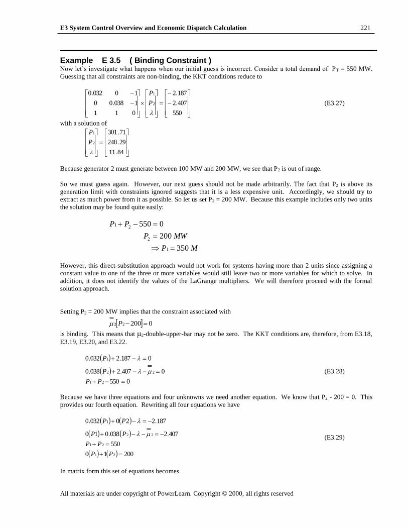
Example E 3.5 ( Binding Constraint ) Now let’s investigate what happens when our initial guess is incorrect. Consider a total demand of PT = 550 MW.

Guessing that all constraints are non-binding, the KKT conditions reduce to

550

407.2

187.2

011

1038.00

10032.0

2

1

P

P

(E3.27)

with a solution of

84.11

29.248

71.301

2

1

P

P

Because generator 2 must generate between 100 MW and 200 MW, we see that P2 is out of range.

So we must guess again. However, our next guess should not be made arbitrarily. The fact that P2 is above its

generation limit with constraints ignored suggests that it is a less expensive unit. Accordingly, we should try to

extract as much power from it as possible. So let us set P2 = 200 MW. Because this example includes only two units

the solution may be found quite easily:

MP

MWP

PP

350

200

0550

1

2

21

However, this direct-substitution approach would not work for systems having more than 2 units since assigning a

constant value to one of the three or more variables would still leave two or more variables for which to solve. In

addition, it does not identify the values of the LaGrange multipliers. We will therefore proceed with the formal

solution approach.

Setting P2 = 200 MW implies that the constraint associated with

020022 P

is binding. This means that μ2-double-upper-bar may not be zero. The KKT conditions are, therefore, from E3.18,

E3.19, E3.20, and E3.22.

0550

0407.2038.0

0187.2032.0

21

22

1

PP

P

P

(E3.28)

Because we have three equations and four unknowns we need another equation. We know that P2 - 200 = 0. This

provides our fourth equation. Rewriting all four equations we have

20010

550

407.2038.010

187.220032.0

21

21

22

1

PP

PP

PP

PP

(E3.29)

In matrix form this set of equations becomes



200

550

407.2

187.2

0010

0011

11038.00

010032.0

2

1

P

P

(E3.30)

The solution is

38.3

39.13

200

350

2

1

P

P

Example E 3.6 (The Meaning of μ) The units of μ are the same as those of λ: $/MWhr. It is important to understand the meaning of

MWhr/$38.32

This is the incremental cost of the constraint associated with the upper limit of unit 2. It indicates the cost of

increasing this limit by 1 MW for the next hour. Since μ2-double-upper-bar is negative, the “cost” is actually a

savings. We can check this conclusion by computing the total system costs when the constraint is 200 MW and

when it is 201 MW. For a total demand of 550 MW with a maximum unit-2 generation capability of 200 MW we

have P1 = 350, P2 = 200 and therefore

Now we need to obtain the total costs for a total demand of 550 MW with an increase in the upper limit of the

second unit, P2, by 1 MW. To do this, we need to re-solve the economic dispatch problem. Since we have already

found the unconstrained problem (refer to Eq. E3.27) to result in P1 = 301.71, P2 = 248.29, we know that the

maximum limit of 201 MW limit will be violated. We simply need to adjust Eq. E3.30, resulting in

201

550

407.2

187.2

0010

0011

11038.00

010032.0

2

1

P

P

with a solution of:

hrPCPCC

hrPC

PC

hrPC

PC

T /$23.416147.131576.2845

/$47.1315

074.74200407.2200019.0

/$76.2845

312.120350187.2350016.0

2211

22

222

11

211

31.3

35.13

201

349

2

1

P

P



The costs for each generator are, then,

hrPCPCC

hrPC

PC

hrPC

PC

T /$89.415750.132539.2832

/$50.1325

074.74201407.2201019.0

/$39.2832

312.120349187.2349016.0

2211

22

222

11

211

The total costs are

89.415750.132539.28322211 PCPCCT

So, as a result of the 1 MW increase in P2max, the total cost will change by

h/$34.323.416189.4157

The small difference between this value and μ-double-upper-bar is due to round-off error and the non-linearity of

the problem.

E3.7.2 Graphical Solution Recall the first KKT condition when applied to the general system eqn.(E3.9) shown again here for convenience:

ni

P

PC

P

Fii

i

ii

i

,100

If we assume that all binding inequality constraints have been converted to equality constraint, so that the mu’s are

zero, then eqn. (E3.32) (above) becomes

Bi

niP

PC

P

F

i

ii

i

,100

where B is the set of all generators without binding constraints. This equation implies that for all regulating

generators (i.e. units not at their limits) each generator’s incremental costs are the same and are equal to λ:

Bini

P

PC

P

PC

P

PC

i

ii

,1

2

22

1

11

This very important principle provides the basis on which to apply the graphical solution method. The graphical

solution is illustrated in Figure E3.6 (note that “ICC” means incremental-cost-curve). The unit's data are simply

plotted adjacent to each other. Then, a value for λ is chosen (judiciously), a “ruler” is placed horizontally across the

graphs at the value of , and the generations are added. If the total generation is equal to the total demand “PT”

then the optimal solution has been found. Otherwise, a new value for λ is chosen and the process repeated. The

limitations of each unit are included as vertical lines since the solution must not include generation beyond unit

capabilities.



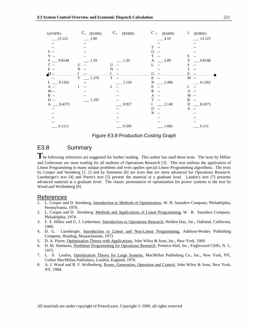
Figure E3.6 Graphical Solution of EDC

Example E 3.7 Our two-unit problem can be solved using a graphical approach as shown in Figure E3.7. The λ axis is on the far

right and is used for all units since all units must have the same value for λ at the optimum solution. The ruler yields

the generation for each unit at the given value of λ and is shown as a line with solid dots at each end. The ruler can

then be used to find the generation for each unit for a given function of λ by moving it up and down. These

generation values are then added to find the total generation. If the total generation is the generation to be

dispatched, then the placement of the ruler is optimal. Otherwise, the ruler has to be moved up if the total

generation is too low, and down if the total generation is too high. To simply the operation, note that the total

generation for each value of λ is shown on the far right. Also the λ axis is provided at both the left and right hand

sides for convenience. A similar production-costing curve is shown in Figure E3.8 with a ruler which would move

in parallel with the above ruler. The solution indicated in Fig E3.7 corresponds to a loading level of about PT = 410

MW, λ = 9.30 $/MWhr, P1 = 223 MW, and P2 = 187 Mw. See if you can verify the solutions found in example 3.3

(PT = 400 MW) and 3.5 (PT = 550 MW).

λ ($/MW) 1P (MW) 2P (MW) TP (MW) ($/MW)

___13.125 ___ 350. ___ 550. ___ 13.125

-- -- -- --

-- -- T -- --

S -- -- O -- --

Y -- -- T -- S --

S ___ 9.8148 ___ 244.1 ___ 200.0 A ___ 444.1 Y ___ 9.8148

T -- U -- U -- L -- S --

E -- N -- N -- -- T --

M -- I -- I -- G -- E --

-- T ___ 222.0 T -- E -- M --

L ___ 9.1262 -- ___ 181.4 N ___ 403.4 ___ 9.1262

A -- 1 -- 2 -- E -- L --

M -- -- -- R -- A --

B -- -- -- A -- M --

D -- ___ 200. -- T -- B --

A ___ 8.4375 ___ 162.8 I ___ 362.8 D ___ 8.4375

-- -- O -- A --

-- -- N -- --

-- -- -- --

-- -- -- --

___ 6.1111 ___ 100. ___ 300. ___ 6.111

Figure E3.7 Economic Dispatch Graphical Solution



λ($/MW) 1C ($1000) 2C ($1000) TC ($1000) ($/MW)

___13.125 ___ 2.80 ___ 4.10 ___ 13.125

-- -- -- --

-- -- T -- --

S -- -- O -- --

Y -- -- T -- S --

S ___ 9.8148 ___ 1.59 ___ 1.30 A ___ 2.89 Y ___ 9.8148

T -- U -- U -- L -- S --

E -- N -- N -- -- T --

M -- I -- I -- G -- E --

-- T ___ 1.376 T -- E -- M --

L ___ 9.1262 -- ___ 1.120 N ___ 2.496 ___ 9.1262

A -- 1 -- 2 -- E -- L --

M -- -- -- R -- A --

B -- -- -- A -- M --

D -- ___ 1.183 -- T -- B --

A ___ 8.4375 ___ 0.957 I ___ 2.140 D ___ 8.4375

-- -- O -- A --

-- -- N -- --

-- -- -- --

-- -- -- --

___ 6.1111 ___ 0.500 ___ 1.683 ___ 6.111

Figure E3.8 Production Costing Graph

E3.8 Summary

The following references are suggested for further reading. This author has used these texts. The texts by Hillier

and Lieberman are must reading for all students of Operations Research [3]. This text outlines the application of

Linear Programming to many unique problems and even applies special Linear Programming algorithms. The texts

by Cooper and Steinberg [1, 2] and by Simmons [6] are texts that are more advanced for Operations Research.

Luenberger's text [4] and Pierre's text [5] present the material at a graduate level. Lasdon's text [7] presents

advanced material at a graduate level. The classic presentation of optimization for power systems is the text by

Wood and Wollenberg [8].

References 1. L. Cooper and D. Steinberg, Introduction to Methods of Optimization, W. B. Saunders Company, Philadelphia,

Pennsylvania, 1970.

2. L. Cooper and D. Steinberg, Methods and Applications of Linear Programming, W. B. Saunders Company,

Philadelphia, 1974.

3. F. S. Hillier and G. J. Lieberman, Introduction to Operations Research, Holden-Day, Inc., Oakland, California,

1986.

4. D. G. Luenberger, Introduction to Linear and Non-Linear Programming, Addison-Wesley Publishing

Company, Reading, Massachusetts, 1973.

5. D. A. Pierre, Optimization Theory with Applications, John Wiley & Sons, Inc., New York, 1969.

6. D. M. Simmons, Nonlinear Programming for Operations Research, Prentice-Hall, Inc., Englewood Cliffs, N. J.,

1975.

7. L. S. Lasdon, Optimization Theory for Large Systems, MacMillan Publishing Co., Inc., New York, NY,

Collier MacMillan Publishers, London, England, 1970.

8. A. J. Wood and B. F. Wollenberg, Power, Generation, Operation and Control, John Wiley & Sons, New York,

NY, 1984.



P R O B L E M S

Problem 1

A two-unit system is given by the following data

37025.0

62015.0

2

2

222

1

2

111

ggg

ggg

PPPC

PPPC

The total system demand is 500MW. The lower and upper limits for each generator unit are 20 and 300MW,

respectively.

(a) Determine the optimal dispatch ignoring inequality constraints

(b) And identify whether it is a feasible dispatch or not (support your answer)

Problem 2

Generator cost rate functions, in $/hr, for a three unit system are given as

2008.5009.0

4005.5006.0

5003.5004.0

3

2

333

2

2

222

1

2

111

PPPC

PPPC

PPPC

Limits on the generation levels are ,450200 1 P ,350150 2 P 225100 3 P . These three generators must

supply a total demand of 975 MW.

(a) Form the linear matrix equation necessary to solve the unconstrained optimization problem.

(b) The solution to the unconstrained optimization problem is ,9.4821 MWP ,3.3052 MWP

.5.1863 MWP For this solution (i.e., ignoring limits)

(i) Compute λ

(ii) Determine the total cost rate

(iii) How much would the total cost rate change if the total load increased from 975 to 976 MW? (Indicate

whether the total cost rate increases or decreases).

(c) Form the linear matrix equation necessary to solve the next iteration of getting the solution to this problem.

Problem 3

A three-unit system is given by the following data. The total system demand is 1100MW. Generator constraints are

5500 1 gP , 3000 2 gP , 3000 3 gP

13.0010.0 1

2

111 ggg PPPC

32.0030.0 2

2

222 ggg PPPC

59.0020.0 3

2

333 ggg PPPC

(a) Identify the objective function for this optimization problem.

(b) Identify the LaGrangian function assuming no constraints are binding.



(c) Identify the KKT conditions assuming no constraints are binding.

(d) Find the solution to the problem assuming no constraints are binding.

(e) Find the solution to the problem accounting for any binding constraints.

(f) Find the total cost of supplying the 1100MW using the solution found in part (e)

(g) Approximately the total cost of supplying the 1100MW change if the upper limit on generator 1 was increased

from 550MW to 560MW.

Problem 4

A three-unit system is given by the following data. The total system demand is 1100MW. Generator constraints are ,7000 1 gP ,2000 2 gP .3.2520 3 gP

55.0008.0 1

2

111 ggg PPPC

32.0030.0 2

2

222 ggg PPPC

5020.0 3

2

333 ggg PPPC

(a) Set up the linear matrix equation to solve the economic dispatch problem, assuming all constraints are satisfied

(i.e., ignore constraints. DO NOT solve the equation.

(b) The solution to the problem in (a) is ,5.6641 MWPg ,2.1822 MWPg and .3.2533 MWPg Reformulate this linear

matrix equation to solve the economic dispatch problem for this system, accounting for any violated constraints.

Again, you DO NOT need to actually solve the equation, just set it up.

(c) Using only the cost function for generator 1, 1g1 PC , together with information given in the part b problem

statement, determine the system λ for the solution to the unconstrained problem.

Problem 5

Recall that the "system λ" is the cost to the system owner of producing the next MW over the next hour; it is equal to

the incremental cost of an individual unit when the system is economically dispatched for minimum cost and the

unit is not at an upper or lower generation limit. A two-unit system is given by the following data.

62015.0 1

2

111 ggg PPPC

46020.0 1

2

222 ggg PPPC

The demand is 300MW

1. Write the KKT conditions that must be satisfied at the optimal solution to this problem, assuming that both units

are operating between their respective upper and lower limits.

2. Set up the linear matrix equation to solve the economic dispatch problem for this system, assuming that both

units are operating between their respective upper and lower limits. Do NOT solve the system of equations.

3. The solution to the problem in (2) is ,57.2281 MWPg MWPg 43.712 . Assuming that each unit has a minimum

generation capability of 80 MW.

(a) Indicate why the given solution is not feasible.

(b) Identify the optimal feasible solution

(c) Identify the incremental costs of each unit at the optimal feasible solution

(d) Identify the system λ at the optimal feasible solution

(e) Would the total cost of supplying the 300MW increase or decrease (relative to the total cost corresponding

to the optimal feasible solution) if the minimum generation capabilities on both units were changed to

79MW?



Problem 6

The ‘system λ’ is the cost to the system owner of producing the next MW over the next hour. It is equal to the

incremental cost of an individual unit when the system is economically dispatched for minimum cost and the unit is

not at an upper or lower generation limit. A three-unit system is given by the following data.

Total system demand is 1000 MW.

5020.0

62015.0

55.0008.0

32

333

22

222

12

111

ggg

ggg

ggg

PPPC

PPPC

PPPC

a) Set up the linear matrix equation to solve the economic dispatch problem for this system. DO NOT

solve the equation.

b) The solution to the problem in (a) is Pg1 = 549.6 MW, Pg2 = 243.1 MW, and Pg3 = 207.3 MW.

Assume that each unit has a maximum generation capability of 350 MW. Reformulate the linear

matrix equation to solve the economic dispatch problem for this system. Again, DO NOT solve the

system.

c) What is the incremental cost for unit 1under the condition specified in part (b)? Do you think the

system λ is greater than or less than this value?

Problem 7

Generator 1 has an incremental cost curve of:

0.205.0 111 gg PPIC

and limits of:

.10010 1 MWPMW g

The generator operates in an economically dispatched system. In this system, it is found that supplying an

additional 5 MW costs an additional $50/hr. Determine Pg1.

Problem 8

A system consists of two generators supplying a load. Generators 1 and 2 have incremental cost curves as indicated

below:

.0.106.0

0.204.0

222

111

gg

gg

PPIC

PPIC

and limits of:

MWPMW

MWPMW

g

g

10030

10010

2

1

a) In this system, when the load is 140 MW, what is the dispatch of these two units?

b) In this system, when the load is 190 MW, what is the dispatch of these two units?

c) In this system, under a certain economically dispatched scenario (a scenario different than in part

(a) and (b)), it is found that supplying an additional 1 MW costs an additional $5.68/hr.

Determine Pg1 and Pg2.



Problem 9

A two unit system has incremental cost curves (the derivatives of the cost curves) of IC1=0.01P1+5, and

IC2=0.02P2+4, where P1 and P2 are given in MW. The demand is 300 MW. Ignoring limits on the generators,

determine the values of P1 and P2 that minimize the cost of supplying the 300 MW.

Problem 10

A two-generator system is operating on economic dispatch and supplying 420 Mw of load. The total cost of supply

is computed from the final EDC solution (i.e., all constraints are satisfied) and found to be $3000/hr. From this same

final solution, the LaGrange multipliers are found to be:

Equality constraint =$15/Mw-hr

Pg1 > 20 Mw 1,L=0

Pg1 < 300 Mw 1,H=0

Pg2 > 10 Mw 2,L=0

Pg2 < 200 Mw 2,H= -$4.00/Mw-hr

Here the subscripts “L” and “H” indicate “Low limit” and “High limit,” respectively, and refer to the corresponding

inequality constraint. For each question below, you must provide some basis or reasoning for your response.

(a) What would be the (approximate) total cost of supply if the total demand was increased to 421 MW?

(b) What would be the total cost of supply if the lower limit for generator 2 was increased from 10 MW to 11

MW?

(c) What would be the total cost of supply if the upper limit for generator 2 was increased from 200 MW to

201 MW?

(d) What are the generation levels in Mw of generators 1 and 2 ?

(e) What is the incremental cost for generator 1?

Problem 11

A two generator system has cost curves ($/hr) of C1(P1)=0.006P12 +5P1+3 , and C2(P2)=0.01P2

2+4P2+2, where P1 and

P2 are given in MW. The total demand is PT=500 MW. The limits on these generators are 0<P1<300 and 0<P2<300.

a. Determine the unconstrained values of P1 and P2 that minimize the cost of supplying the 500 MW, and

indicate whether this solution is feasible or not.

b. For the solution found in (a), how much would the total cost of supply change if the total demand increased

to 501 MW for one hour ?

c. Use the complementary condition (the third condition in the KKT conditions), to identify the values of each

Lagrange multiplier associated with the inequality constraints.

Date post:	28-Aug-2018
Category:	Documents
Upload:	voliem
View:	220 times
Download:	0 times

E3 System Control Overview and Economic Dispatch...

Documents