EA-4 02 M: 1999 Expression of the Uncertainty of Measurement in Calibration · the uncertainty of...

EA-4/02 • Expression of the Uncertainty of Measurement in Calibration

December 1999 rev00 page 1 of 79

Publication Reference

PURPOSE The purpose of this document is to harmonise evaluation of uncertainty of measurement within EA, to set up, in addition to the general requirements of EAL-R1, the specific demands in reporting uncertainty of measurement on calibration certificates issued by accredited laboratories and to assist accreditation bodies with a coherent assignment of best measurement capability to calibration laboratories accredited by them. As the rules laid down in this document are in compliance with the recommendations of the Guide to the Expression of Uncertainty in Measurement, published by seven international organisations concerned with standardisation and metrology, the implementation of EA-4/02 will also foster the global acceptance of European results of measurement.

EA-4/02 M: 1999

Measurement in Calibration

Expression of the

Uncertainty of


December 1999 rev00 Page 2 of 79

Authorship This document has been drafted by EAL Task Force for revision of WECC Doc. 19-1990 on behalf of the EAL Committee 2 (Calibration and Testing Activities). It comprises a thorough revision of WECC Doc. 19-1990 which it replaces.

Official language The text may be translated into other languages as required. The English language version remains the definitive version.

Copyright The copyright of this text is held by EA. The text may not be copied for resale.

Further information For further information about this publication, contact your National member of EA. You will find the list of members at the web-site: www.european-accreditation.org Category: Application documents and Technical Adcvisory documents for

Conformity Assessment Bodies EA-4/02 is mandatory document Date of Approval: December 1999 Date of Implementation: December 2000 Transitional Period: one year

http://www.european-accreditation.org/



CONTENTS

1 INTRODUCTION 4

2 OUTLINE AND DEFINITIONS 4

3 EVALUATION OF UNCERTAINTY OF MEASUREMENT OF INPUT ESTIMATES 6

4 CALCULATION OF THE STANDARD UNCERTAINTY OF THE OUTPUT ESTIMATE 8

5 EXPANDED UNCERTAINTY OF MEASUREMENT 11

6 STATEMENT OF UNCERTAINTY OF MEASUREMENT IN CALIBRATION CERTIFICATES 12

7 STEP-BY-STEP PROCEDURE FOR CALCULATING THE UNCERTAINTY OF MEASUREMENT 13

8 REFERENCES 13

APPENDIX A 15

APPENDIX B 18

APPENDIX C 20

APPENDIX D 21

APPENDIX E 24

SUPPLEMENT 1 27

SUPPLEMENT 2 51



1 INTRODUCTION

1.1 This document sets down the principles of and the requirements on the evaluation of the uncertainty of measurement in calibration and the statement of this uncertainty in calibration certificates. The treatment is kept on a general level to suit all fields of calibration. The method outlined may have to be supplemented by more specific advice for different fields, to make the information more readily applicable. In developing such supplementary guidelines the general principles stated in this document should be followed to ensure harmonisation between the different fields.

1.2 The treatment in this document is in accordance with the Guide to the Expression of

Uncertainty in Measurement, first published in 1993 in the name of BIPM, IEC, IFCC, ISO, IUPAC, IUPAP and OIML [ref. 1]. But whereas [ref. 1] establishes general rules for evaluating and expressing uncertainty in measurement that can be followed in most fields of physical measurements, this document concentrates on the method most suitable for the measurements in calibration laboratories and describes an unambiguous and harmonised way of evaluating and stating the uncertainty of measurement. It comprises the following subjects:

definitions basic to the document;

methods for evaluating the uncertainty of measurement of input quantities;

relationship between the uncertainty of measurement of the output quantity and the uncertainty of measurement of the input quantities;

expanded uncertainty of measurement of the output quantity;

statement of the uncertainty of measurement;

a step by step procedure for calculating the uncertainty of measurement. Worked out examples showing the application of the method outlined here to specific measurement problems in different fields will be given in supplements. Evaluation of uncertainty of measurement is also addressed in several of the EAL documents which provide guidance on calibration methods, some of these documents containing specific worked out examples.

1.3 Within EAL the best measurement capability (always referring to a particular

quantity, viz. the measurand) is defined as the smallest uncertainty of measurement that a laboratory can achieve within its scope of accreditation, when performing more or less routine calibrations of nearly ideal measurement standards intended to define, realize, conserve or reproduce a unit of that quantity or one or more of its values, or when performing more or less routine calibrations of nearly ideal measuring instruments designed for the measurement of that quantity. The assessment of best measurement capability of accredited calibration laboratories has to be based on the method described in this document but shall normally be supported or confirmed by experimental evidence. To assist accreditation bodies with the assessment of the best measurement capability some further explanations are given in Annex A.

2 OUTLINE AND DEFINITIONS

Note: Terms of special relevance to the context of the main text are written in bold when they appear for the first time in this document. Appendix B contains a glossary of these terms together with references



2.1 The statement of the result of a measurement is complete only if it contains both the value attributed to the measurand and the uncertainty of measurement associated with that value. In this document all quantities which are not exactly known are treated as random variables, including the influence quantities which may affect the measured value.

2.2 The uncertainty of measurement is a parameter, associated with the result of a measurement, that characterises the dispersion of the values that could reasonably be attributed to the measurand [ref. 2]. In this document the shorthand term uncertainty is used for uncertainty of measurement if there is no risk of misunderstanding. For typical sources of uncertainty in a measurement see the list given in Annex C.

2.3 The measurands are the particular quantities subject to measurement. In

calibration one usually deals with only one measurand or output quantity Y that depends upon a number of input quantities Xi (i = 1, 2 ,…, N) according to the functional relationship

Y = f(X1, X2, …, XN

) (2.1)

The model function f represents the procedure of the measurement and the method of evaluation. It describes how values of the output quantity Y are obtained from values of the input quantities Xi. In most cases it will be an analytical expression, but it may also be a group of such expressions which include corrections and correction factors for systematic effects, thereby leading to a more complicated relationship that is not written down as one function explicitly. Further, f may be determined experimentally, or exist only as a computer algorithm that must be evaluated numerically, or it may be a combination of all of these.

2.4 The set of input quantities Xi may be grouped into two categories according to the way in which the value of the quantity and its associated uncertainty have been determined:

(a) quantities whose estimate and associated uncertainty are directly determined in the current measurement. These values may be obtained, for example, from a single observation, repeated observations, or judgement based on experience. They may involve the determination of corrections to instrument readings as well as corrections for influence quantities, such as ambient temperature, barometric pressure or humidity;

(b) quantities whose estimate and associated uncertainty are brought into the measurement from external sources, such as quantities associated with calibrated measurement standards, certified reference materials or reference data obtained from handbooks.

2.5 An estimate of the measurand Y, the output estimate denoted by y, is obtained from equation (2.1) using input estimates xi for the values of the input quantities Xi

y f x x xN ( , ,.., )1 2 (2.2)

It is understood that the input values are best estimates that have been corrected for all effects significant for the model. If not, the necessary corrections have been introduced as separate input quantities.



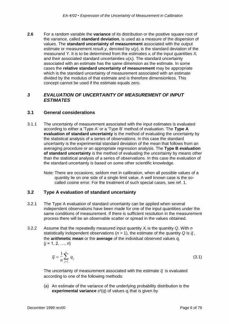
2.6 For a random variable the variance of its distribution or the positive square root of

the variance, called standard deviation, is used as a measure of the dispersion of values. The standard uncertainty of measurement associated with the output estimate or measurement result y, denoted by u(y), is the standard deviation of the measurand Y. It is to be determined from the estimates xi of the input quantities Xi and their associated standard uncertainties u(xi). The standard uncertainty associated with an estimate has the same dimension as the estimate. In some cases the relative standard uncertainty of measurement may be appropriate which is the standard uncertainty of measurement associated with an estimate divided by the modulus of that estimate and is therefore dimensionless. This concept cannot be used if the estimate equals zero.

3 EVALUATION OF UNCERTAINTY OF MEASUREMENT OF INPUT ESTIMATES

3.1 General considerations

3.1.1 The uncertainty of measurement associated with the input estimates is evaluated

according to either a 'Type A' or a 'Type B' method of evaluation. The Type A evaluation of standard uncertainty is the method of evaluating the uncertainty by the statistical analysis of a series of observations. In this case the standard uncertainty is the experimental standard deviation of the mean that follows from an averaging procedure or an appropriate regression analysis. The Type B evaluation of standard uncertainty is the method of evaluating the uncertainty by means other than the statistical analysis of a series of observations. In this case the evaluation of the standard uncertainty is based on some other scientific knowledge. Note: There are occasions, seldom met in calibration, when all possible values of a

quantity lie on one side of a single limit value. A well known case is the so-called cosine error. For the treatment of such special cases, see ref. 1.

3.2 Type A evaluation of standard uncertainty

3.2.1 The Type A evaluation of standard uncertainty can be applied when several

independent observations have been made for one of the input quantities under the same conditions of measurement. If there is sufficient resolution in the measurement process there will be an observable scatter or spread in the values obtained.

3.2.2 Assume that the repeatedly measured input quantity Xi is the quantity Q. With n statistically independent observations (n > 1), the estimate of the quantity Q is q ,

the arithmetic mean or the average of the individual observed values qj (j = 1, 2, …, n)

qn

q jj

n

1

1

(3.1)

The uncertainty of measurement associated with the estimate q is evaluated

according to one of the following methods: (a) An estimate of the variance of the underlying probability distribution is the

experimental variance s²(q) of values qj that is given by



s qn

q qjj

n2

1

21

1( ) ( )

(3.2)

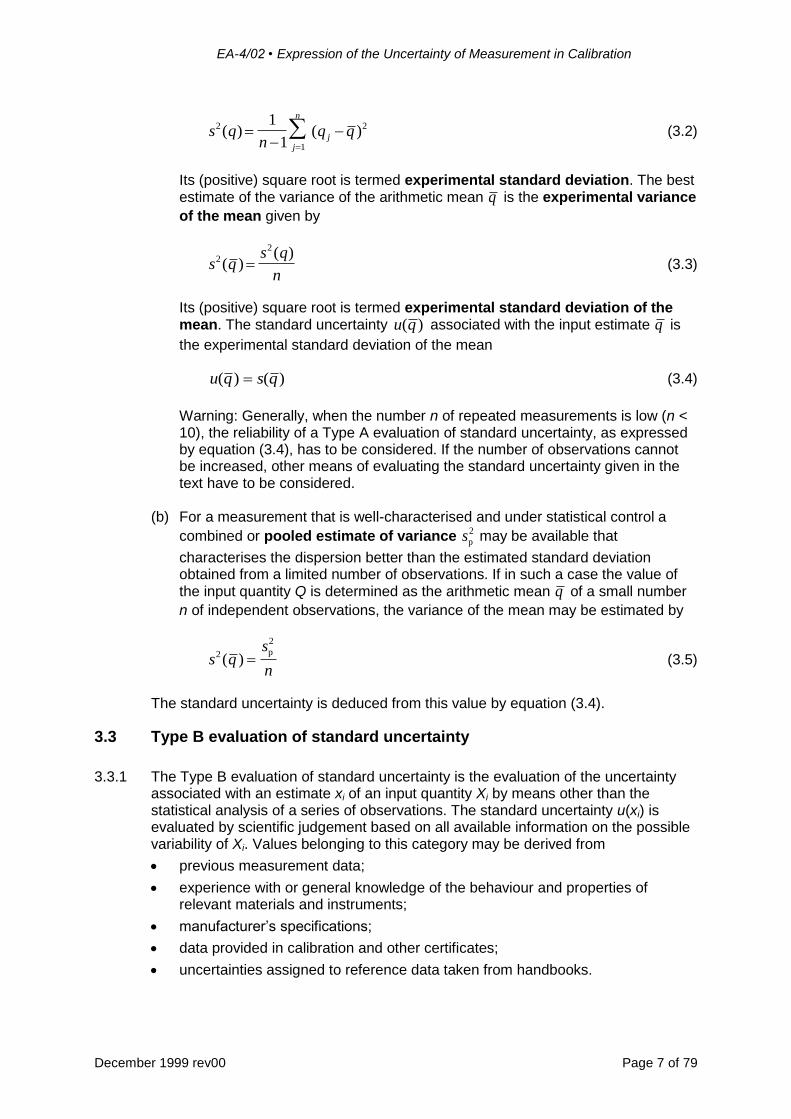
Its (positive) square root is termed experimental standard deviation. The best estimate of the variance of the arithmetic mean q is the experimental variance

of the mean given by

s qs q

n

2

2

( )( )

(3.3)

Its (positive) square root is termed experimental standard deviation of the mean. The standard uncertainty u q( ) associated with the input estimate q is

the experimental standard deviation of the mean

u q s q( ) ( ) (3.4)

Warning: Generally, when the number n of repeated measurements is low (n < 10), the reliability of a Type A evaluation of standard uncertainty, as expressed by equation (3.4), has to be considered. If the number of observations cannot be increased, other means of evaluating the standard uncertainty given in the text have to be considered.

(b) For a measurement that is well-characterised and under statistical control a

combined or pooled estimate of variance sp

2 may be available that

characterises the dispersion better than the estimated standard deviation obtained from a limited number of observations. If in such a case the value of the input quantity Q is determined as the arithmetic mean q of a small number

n of independent observations, the variance of the mean may be estimated by

s qs

n

2

2

( )p

(3.5)

The standard uncertainty is deduced from this value by equation (3.4).

3.3 Type B evaluation of standard uncertainty

3.3.1 The Type B evaluation of standard uncertainty is the evaluation of the uncertainty

associated with an estimate xi of an input quantity Xi by means other than the statistical analysis of a series of observations. The standard uncertainty u(xi) is evaluated by scientific judgement based on all available information on the possible variability of Xi. Values belonging to this category may be derived from

previous measurement data;

experience with or general knowledge of the behaviour and properties of relevant materials and instruments;

manufacturer’s specifications;

data provided in calibration and other certificates;

uncertainties assigned to reference data taken from handbooks.



3.3.2 The proper use of the available information for a Type B evaluation of standard uncertainty of measurement calls for insight based on experience and general knowledge. It is a skill that can be learned with practice. A well-based Type B evaluation of standard uncertainty can be as reliable as a Type A evaluation of standard uncertainty, especially in a measurement situation where a Type A evaluation is based only on a comparatively small number of statistically independent observations. The following cases must be discerned:

(a) When only a single value is known for the quantity Xi, e.g. a single measured value, a resultant value of a previous measurement, a reference value from the literature, or a correction value, this value will be used for xi. The standard uncertainty u(xi) associated with xi is to be adopted where it is given. Otherwise it has to be calculated from unequivocal uncertainty data. If data of this kind are not available, the uncertainty has to be evaluated on the basis of experience.

(b) When a probability distribution can be assumed for the quantity Xi, based on theory or experience, then the appropriate expectation or expected value and the square root of the variance of this distribution have to be taken as the estimate xi and the associated standard uncertainty u(xi), respectively.

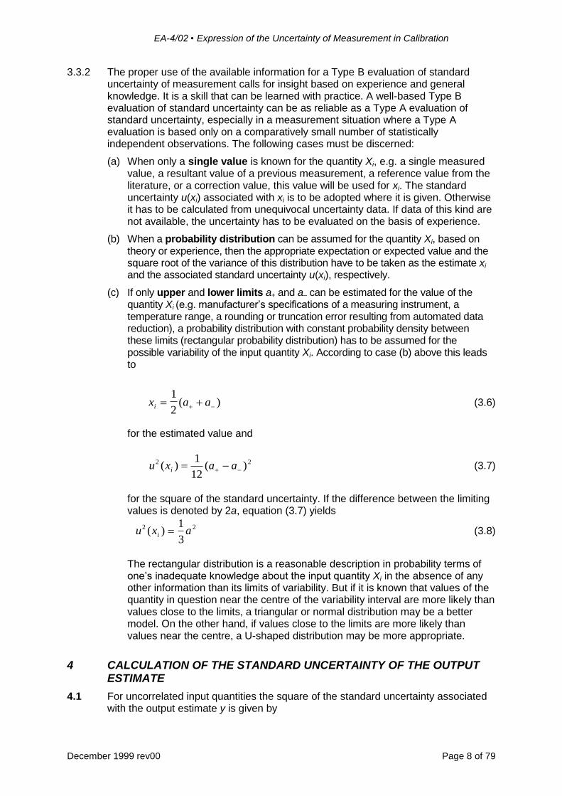
(c) If only upper and lower limits a+ and a– can be estimated for the value of the quantity Xi (e.g. manufacturer’s specifications of a measuring instrument, a temperature range, a rounding or truncation error resulting from automated data reduction), a probability distribution with constant probability density between these limits (rectangular probability distribution) has to be assumed for the possible variability of the input quantity Xi. According to case (b) above this leads to

x a ai

1

2( ) (3.6)

for the estimated value and

u x a ai

2 21

12( ) ( ) (3.7)

for the square of the standard uncertainty. If the difference between the limiting values is denoted by 2a, equation (3.7) yields

u x ai

2 21

3( ) (3.8)

The rectangular distribution is a reasonable description in probability terms of one’s inadequate knowledge about the input quantity Xi in the absence of any other information than its limits of variability. But if it is known that values of the quantity in question near the centre of the variability interval are more likely than values close to the limits, a triangular or normal distribution may be a better model. On the other hand, if values close to the limits are more likely than values near the centre, a U-shaped distribution may be more appropriate.

4 CALCULATION OF THE STANDARD UNCERTAINTY OF THE OUTPUT ESTIMATE

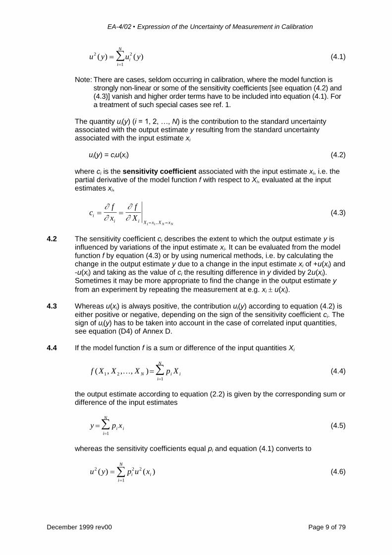
4.1 For uncorrelated input quantities the square of the standard uncertainty associated with the output estimate y is given by



u y u yii

N2 2

1

( ) ( )

(4.1)

Note: There are cases, seldom occurring in calibration, where the model function is

strongly non-linear or some of the sensitivity coefficients [see equation (4.2) and (4.3)] vanish and higher order terms have to be included into equation (4.1). For a treatment of such special cases see ref. 1.

The quantity ui(y) (i = 1, 2, …, N) is the contribution to the standard uncertainty associated with the output estimate y resulting from the standard uncertainty associated with the input estimate xi

ui(y) = ciu(xi) (4.2) where ci is the sensitivity coefficient associated with the input estimate xi, i.e. the partial derivative of the model function f with respect to Xi, evaluated at the input estimates xi,

cf

x

f

Xi

i i X x X xN N

1 1 ..

(4.3)

4.2 The sensitivity coefficient ci describes the extent to which the output estimate y is

influenced by variations of the input estimate xi. It can be evaluated from the model function f by equation (4.3) or by using numerical methods, i.e. by calculating the change in the output estimate y due to a change in the input estimate xi of +u(xi) and -u(xi) and taking as the value of ci the resulting difference in y divided by 2u(xi). Sometimes it may be more appropriate to find the change in the output estimate y

from an experiment by repeating the measurement at e.g. xi u(xi).

4.3 Whereas u(xi) is always positive, the contribution ui(y) according to equation (4.2) is either positive or negative, depending on the sign of the sensitivity coefficient ci. The sign of ui(y) has to be taken into account in the case of correlated input quantities, see equation (D4) of Annex D.

4.4 If the model function f is a sum or difference of the input quantities Xi

f X X X p XN i ii

N

( , , , )1 21

(4.4)

the output estimate according to equation (2.2) is given by the corresponding sum or difference of the input estimates

y p xi ii

N

1

(4.5)

whereas the sensitivity coefficients equal pi and equation (4.1) converts to

u y p u xi i

i

N2 2 2

1

( ) ( )

(4.6)



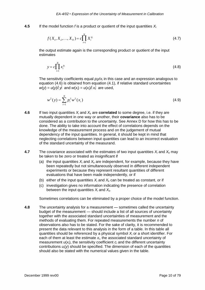
4.5 If the model function f is a product or quotient of the input quantities Xi

f X X X c XN i

p

i

N

i( , , , )1 21

(4.7)

the output estimate again is the corresponding product or quotient of the input estimates

y c xi

p

i

N

i

1

(4.8)

The sensitivity coefficients equal piy/xi in this case and an expression analogous to equation (4.6) is obtained from equation (4.1), if relative standard uncertainties

w(y) = u(y)/y and w(xi) = u(xi)/xi are used,

w y p w xi i

i

N2 2 2

1

( ) ( )

(4.9)

4.6 If two input quantities Xi and Xk are correlated to some degree, i.e. if they are

mutually dependent in one way or another, their covariance also has to be considered as a contribution to the uncertainty. See Annex D for how this has to be done. The ability to take into account the effect of correlations depends on the knowledge of the measurement process and on the judgement of mutual dependency of the input quantities. In general, it should be kept in mind that neglecting correlations between input quantities can lead to an incorrect evaluation of the standard uncertainty of the measurand.

4.7 The covariance associated with the estimates of two input quantities Xi and Xk may be taken to be zero or treated as insignificant if

(a) the input quantities Xi and Xk are independent, for example, because they have been repeatedly but not simultaneously observed in different independent experiments or because they represent resultant quantities of different evaluations that have been made independently, or if

(b) either of the input quantities Xi and Xk can be treated as constant, or if

(c) investigation gives no information indicating the presence of correlation between the input quantities Xi and Xk.

Sometimes correlations can be eliminated by a proper choice of the model function.

4.8 The uncertainty analysis for a measurement — sometimes called the uncertainty budget of the measurement — should include a list of all sources of uncertainty together with the associated standard uncertainties of measurement and the methods of evaluating them. For repeated measurements the number n of observations also has to be stated. For the sake of clarity, it is recommended to present the data relevant to this analysis in the form of a table. In this table all quantities should be referenced by a physical symbol Xi or a short identifier. For each of them at least the estimate xi, the associated standard uncertainty of measurement u(xi), the sensitivity coefficient ci and the different uncertainty contributions ui(y) should be specified. The dimension of each of the quantities should also be stated with the numerical values given in the table.



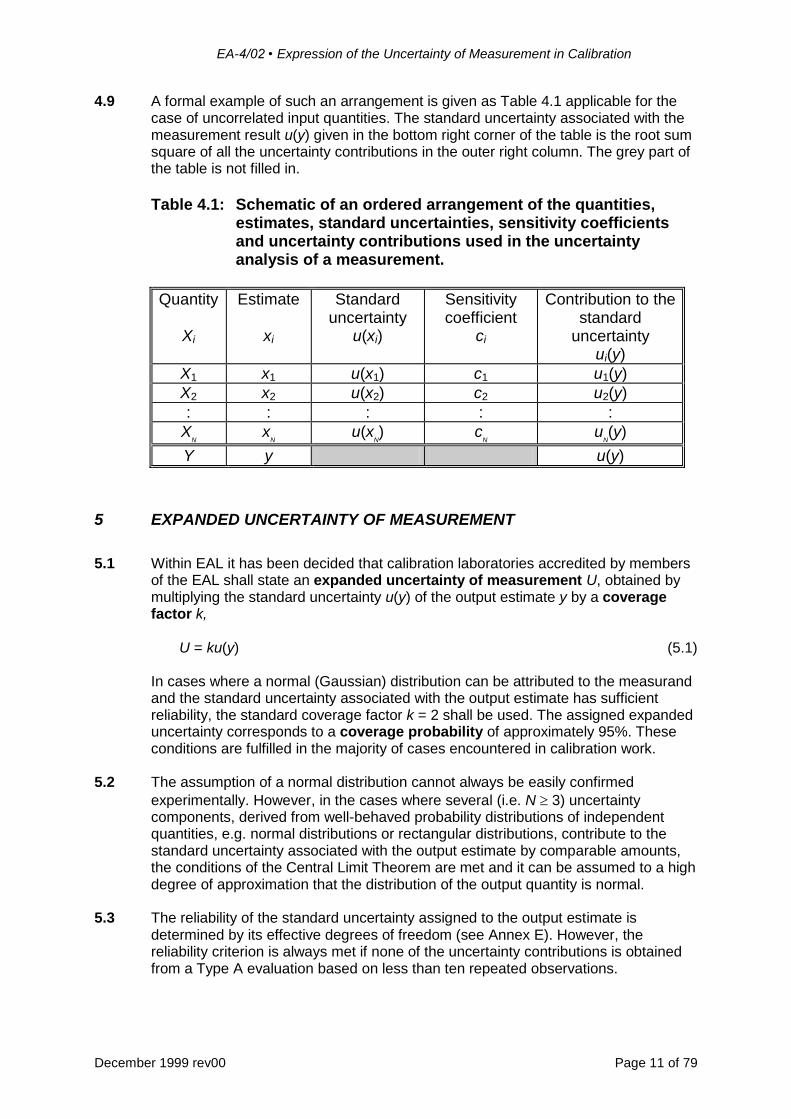
4.9 A formal example of such an arrangement is given as Table 4.1 applicable for the case of uncorrelated input quantities. The standard uncertainty associated with the measurement result u(y) given in the bottom right corner of the table is the root sum square of all the uncertainty contributions in the outer right column. The grey part of the table is not filled in.

Table 4.1: Schematic of an ordered arrangement of the quantities,

estimates, standard uncertainties, sensitivity coefficients and uncertainty contributions used in the uncertainty analysis of a measurement.

Quantity

Xi

Estimate

xi

Standard uncertainty

u(xi)

Sensitivity coefficient

ci

Contribution to the standard

uncertainty ui(y)

X1 x1 u(x1) c1 u1(y)

X2 x2 u(x2) c2 u2(y)

: : : : :

XN x

N u(x

N) c

N u

N(y)

Y y u(y)

5 EXPANDED UNCERTAINTY OF MEASUREMENT

5.1 Within EAL it has been decided that calibration laboratories accredited by members

of the EAL shall state an expanded uncertainty of measurement U, obtained by multiplying the standard uncertainty u(y) of the output estimate y by a coverage factor k,

U = ku(y) (5.1) In cases where a normal (Gaussian) distribution can be attributed to the measurand and the standard uncertainty associated with the output estimate has sufficient reliability, the standard coverage factor k = 2 shall be used. The assigned expanded uncertainty corresponds to a coverage probability of approximately 95%. These conditions are fulfilled in the majority of cases encountered in calibration work.

5.2 The assumption of a normal distribution cannot always be easily confirmed

experimentally. However, in the cases where several (i.e. N 3) uncertainty components, derived from well-behaved probability distributions of independent quantities, e.g. normal distributions or rectangular distributions, contribute to the standard uncertainty associated with the output estimate by comparable amounts, the conditions of the Central Limit Theorem are met and it can be assumed to a high degree of approximation that the distribution of the output quantity is normal.

5.3 The reliability of the standard uncertainty assigned to the output estimate is determined by its effective degrees of freedom (see Annex E). However, the reliability criterion is always met if none of the uncertainty contributions is obtained from a Type A evaluation based on less than ten repeated observations.



5.4 If one of these conditions (normality or sufficient reliability) is not fulfilled, the standard coverage factor k = 2 can yield an expanded uncertainty corresponding to a coverage probability of less than 95%. In these cases, in order to ensure that a value of the expanded uncertainty is quoted corresponding to the same coverage probability as in the normal case, other procedures have to be followed. The use of approximately the same coverage probability is essential whenever two results of measurement of the same quantity have to be compared, e.g. when evaluating the results of an inter-laboratory comparison or assessing compliance with a specification.

5.5 Even if a normal distribution can be assumed, it may still occur that the standard uncertainty associated with the output estimate is of insufficient reliability. If, in this case, it is not expedient to increase the number n of repeated measurements or to use a Type B evaluation instead of the Type A evaluation of poor reliability, the method given in Annex E should be used.

5.6 For the remaining cases, i.e. all cases where the assumption of a normal distribution cannot be justified, information on the actual probability distribution of the output estimate must be used to obtain a value of the coverage factor k that corresponds to a coverage probability of approximately 95%.

6 STATEMENT OF UNCERTAINTY OF MEASUREMENT IN CALIBRATION CERTIFICATES

6.1 In calibration certificates the complete result of the measurement consisting of the

estimate y of the measurand and the associated expanded uncertainty U shall be

given in the form (y U). To this an explanatory note must be added which in the general case should have the following content:

The reported expanded uncertainty of measurement is stated as the standard uncertainty of measurement multiplied by the coverage factor k = 2, which for a normal distribution corresponds to a coverage probability of approximately 95%. The standard uncertainty of measurement has been determined in accordance with EAL Publication EAL-R2.

6.2 However, in cases where the procedure of Annex E has been followed, the

additional note should read as follows:

The reported expanded uncertainty of measurement is stated as the standard uncertainty of measurement multiplied by the coverage factor k = XX, which for

a t-distribution with eff = YY effective degrees of freedom corresponds to a coverage probability of approximately 95%. The standard uncertainty of measurement has been determined in accordance with EAL Publication EAL-R2.

6.3 The numerical value of the uncertainty of measurement should be given to at most

two significant figures. The numerical value of the measurement result should in the final statement normally be rounded to the least significant figure in the value of the expanded uncertainty assigned to the measurement result. For the process of rounding, the usual rules for rounding of numbers have to be used (for further details on rounding see ISO 31-0:1992, Annex B). However, if the rounding brings the numerical value of the uncertainty of measurement down by more than 5%, the rounded up value should be used.



7 STEP-BY-STEP PROCEDURE FOR CALCULATING THE UNCERTAINTY OF MEASUREMENT

7.1 The following is a guide to the use of this document in practice (cf. worked examples in Annex F and in separate supplementary documents):

(a) Express in mathematical terms the dependence of the measurand (output quantity) Y on the input quantities Xi according to equation (2.1). In the case of a direct comparison of two standards the equation may be very simple, e.g. Y = X1+X2.

(b) Identify and apply all significant corrections.

(c) List all sources of uncertainty in the form of an uncertainty analysis in accordance with Section 4.

(d) Calculate the standard uncertainty u q( ) for repeatedly measured quantities in

accordance with sub-section 3.2.

(e) For single values, e.g. resultant values of previous measurements, correction values or values from the literature, adopt the standard uncertainty where it is given or can be calculated according to paragraph 3.3.2 (a). Pay attention to the uncertainty representation used. If no data are available from which the standard uncertainty can be derived, state a value of u(xi) on the basis of scientific experience.

(f) For input quantities for which the probability distribution is known or can be assumed, calculate the expectation and the standard uncertainty u(xi) according to paragraph 3.3.2 (b). If only upper and lower limits are given or can be estimated, calculate the standard uncertainty u(xi) in accordance with paragraph 3.3.2 (c).

(g) Calculate for each input quantity Xi the contribution ui(y) to the uncertainty associated with the output estimate resulting from the input estimate xi according to equations (4.2) and (4.3) and sum their squares as described in equation (4.1) to obtain the square of the standard uncertainty u(y) of the measurand. If input quantities are known to be correlated, apply the procedure given in Annex D.

(h) Calculate the expanded uncertainty U by multiplying the standard uncertainty u(y) associated with the output estimate by a coverage factor k chosen in accordance with Section 5.

(i) Report the result of the measurement comprising the estimate y of the measurand, the associated expanded uncertainty U and the coverage factor k in the calibration certificate in accordance with Section 6.

8 REFERENCES

[1] Guide to the Expression of Uncertainty in Measurement, first edition, 1993, corrected and reprinted 1995, International Organization for Standardization (Geneva, Switzerland).

[2] International Vocabulary of Basic and General Terms in Metrology, second edition, 1993, International Organization for Standardization (Geneva, Switzerland).



[3] International Standard ISO 3534-1, Statistics - Vocabulary and symbols - Part I: Probability and General Statistical Terms, first edition, 1993, International Organization for Standardization (Geneva, Switzerland).



APPENDIX A

Comments on the assessment of best measurement capability

A1 Best measurement capability (see Section 1 of the main text) is one of the parameters that is used to define the scope of an accredited calibration laboratory, the others being physical quantity, calibration method or type of instrument to be calibrated and measurement range. Best measurement capability is normally stated in the accreditation schedule or in other documentation that supports either the decision on accreditation or the accreditation certificate which in many cases is issued as evidence of accreditation. Occasionally it is stated both in the accreditation schedule and in the supporting documents. Best measurement capability is one of the essential pieces of information to be found in directories of accredited laboratories that are regularly issued by accreditation bodies and is used by potential customers to accredited laboratories to judge the suitability of a laboratory to carry out particular calibration work at the laboratory or on site.

A2 To make it possible to compare the capabilities of different calibration laboratories, in particular laboratories accredited by different accreditation bodies, the statement of best measurement capability needs to be harmonised. To facilitate this, some explanations are given below to the term best measurement capability, based on its definition as reported in the main text.

A3 With 'more or less routine calibrations' is meant that the laboratory shall be able to achieve the stated capability in the normal work that it performs under its accreditation. Obviously there are instances where the laboratory would be able to do better as a result of extensive investigations and additional precautions but these cases are not covered by the definition of best measurement capability, unless it is the outspoken policy of the laboratory to perform such scientific investigations (in which case these become the 'more or less routine' type calibrations of the laboratory).

A4 Inclusion of the qualifier 'nearly ideal' in the definition means that best measurement capability should not be dependent on the characteristics of the device to be calibrated. Inherent in the concept of being nearly ideal is thus that there should be no significant contribution to the uncertainty of measurement attributable to physical effects that can be ascribed to imperfections of the device to be calibrated. However, it should be understood that such a device should be available. If it is established that, in a particular case, even the most 'ideal' available device contributes to the uncertainty of measurement, this contribution shall be included in the determination of the best measurement capability and a statement should be made that the best measurement capability refers to calibration of that type of device.

A5 The definition of best measurement capability implies that within its accreditation a laboratory is not entitled to claim a smaller uncertainty of measurement than the best measurement capability. This means that the laboratory shall be required to state a larger uncertainty than that corresponding to the best measurement capability whenever it is established that the actual calibration process adds significantly to the uncertainty of measurement. Typically the equipment under calibration may give a contribution. Obviously the actual uncertainty of measurement can



never be smaller than the best measurement capability. When stating the actual uncertainty, the laboratory shall be asked to apply the principles of the present document.

A6 It should be pointed out that according to the definition of best measurement capability the concept is applicable only to results for which the laboratory claims its status as accredited laboratory. Thus, strictly speaking the term is of an administrative character and does not necessarily need to reflect the real technical capability of the laboratory. It should be possible for a laboratory to apply for accreditation with a larger uncertainty of measurement than its technical capability if the laboratory has internal reasons for doing so. Such internal reasons usually involve cases where the real capability has to be held in confidence to external customers, e.g. when doing research and development work or when providing service to special customers. The policy of the accreditation body should be to grant accreditation on any applied level if the laboratory is capable of carrying out calibrations on that level. (This consideration refers not only to the best measurement capability but to all parameters that define the scope of a calibration laboratory.)

A7 Assessment of best measurement capability is the task of the accreditation body. The estimation of the uncertainty of measurement that defines the best measurement capability should follow the procedure laid down in the present document, with the exception of the case covered in the previous sub-section. The best measurement capability shall be stated to the same level as required for calibration certificates, i.e. in the form of an expanded uncertainty of measurement, normally with coverage factor k = 2. (Only in those exceptional cases where the existence of a normal distribution cannot be assumed or the assessment is based on limited data, the best measurement capability has to be stated to a coverage probability of approximately 95%. See Section 5 of the main text.)

A8 All components contributing significantly to the uncertainty of measurement shall be taken into account when evaluating the best measurement capability. The evaluation of the contributions that are known to vary with time or with any other physical quantity can be based on limits of possible variations assumed to occur under normal working conditions. For instance, if the used working standard is known to drift, the contribution caused by the drift between subsequent calibrations of the standard has to be taken into account when estimating the uncertainty contribution of the working standard.

A9 In some fields the uncertainty of measurement may depend on some additional parameter, e.g. frequency of applied voltage when calibrating standard resistors. Such additional parameters shall be stated together with the physical quantity in question and the best measurement capability specified for the additional parameters. Often this can be done by giving the best measurement capability as a function of these parameters.

A10 The best measurement capability should normally be stated numerically. Where the best measurement capability is a function of the quantity to which it refers (or any other parameter) it should be given in analytical form but in this case it may be illustrative to support the statement by a diagram. It should always be unequivocally clear whether the best measurement capability is given in absolute or relative terms. (Usually the inclusion of the relevant unit gives the necessary explanation but in case of dimensionless quantities a separate statement is needed.)



A11 Although the assessment should be based on the procedures of this document, in the main text there is the requirement that the assessment normally shall be 'supported or confirmed by experimental evidence'. The meaning of this requirement is that the accreditation body should not rely on an evaluation of the uncertainty of measurement only. Interlaboratory comparisons that substantiate the evaluation have to be carried out under the supervision of the accreditation body or on its behalf.



APPENDIX B

Glossary of some relevant terms

B1 arithmetic mean ([ref. 3] term 2.26) The sum of values divided by the number of values

B2 best measurement capability (Section 1) The smallest uncertainty of measurement that a laboratory can achieve within its scope of accreditation, when performing more or less routine calibrations of nearly ideal measurement standards intended to define, realise, conserve or reproduce a unit of that quantity or one or more of its values, or when performing more or less routine calibrations of nearly ideal measuring instruments designed for the measurement of that quantity.

B3 correlation ([ref. 3] term 1.13) The relationship between two or several random variables within a distribution of two or more random variables

B4 correlation coefficient (from [ref. 1] Section C.3.6) The measure of the relative mutual dependence of two random variables, equal to the ratio of their covariance to the positive square root of the product of their variances

B5 covariance (from [ref. 1] Section C.3.4) The measure of the mutual dependence of two random variables, equal to the expectation of the product of the deviations of two random variables from their respective expectations

B6 coverage factor ([ref. 1] term 2.3.6) A numerical factor used as a multiplier of the standard uncertainty of measurement in order to obtain an expanded uncertainty of measurement

B7 coverage probability (from [ref. 1] term 2.3.5, NOTE 1) The fraction, usually large, of the distribution of values that as a result of a measurement could reasonably be attributed to the measurand

B8 experimental standard deviation ([ref. 2] term 3.8) The positive square root of the experimental variance.

B9 expanded uncertainty ([ref. 1] term 2.3.5) A quantity defining an interval about the result of a measurement that may be expected to encompass a large fraction of the distribution of values that could reasonably be attributed to the measurand.

B10 experimental variance (from [ref. 1] Section 4.2.2) The quantity characterising the dispersion of the results of a series of n observations of the same measurand given by equation (3.2) in the text.

B11 input estimate (from [ref. 1] Section 4.1.4) The estimate of an input quantity used in the evaluation of the result of a measurement.

B12 input quantity (from [ref. 1] Section 4.1.2) A quantity on which the measurand depends, taken into account in the process of evaluating the result of a measurement.

B13 measurand ([ref. 2] term 2.6) The particular quantity subject to measurement.



B14 output estimate (from [ref. 1] Section 4.1.4) The result of a measurement calculated from the input estimates by the model function.

B15 output quantity (from [ref. 1] Section 4.1.2) The quantity that represents the measurand in the evaluation of a measurement.

B16 pooled estimate of variance (from [ref. 1] Section 4.2.4) An estimate of the experimental variance obtained from long series of observations of the same measurand in well-characterised measurements under statistical control.

B17 probability distribution ([ref. 3] term 1.3) A function giving the probability that a random variable takes any given value or belongs to a given set of values

B18 random variable ([ref. 3] term 1.2) A variable that may take any of the values of a specified set of values and with which is associated a probability distribution.

B19 relative standard uncertainty of measurement (from [ref. 1] Section 5.1.6) The standard uncertainty of a quantity divided by the estimate of that quantity.

B20 sensitivity coefficient associated with an input estimate (from [ref. 1] Section 5.1.3) The differential change in the output estimate generated by a differential change in an input estimate divided by the change in that input estimate.

B21 standard deviation (from [ref. 3] term 1.23) The positive square root of the variance of a random variable.

B22 standard uncertainty of measurement ([ref. 1] term 2.3.1) The uncertainty of measurement expressed as the standard deviation

B23 Type A evaluation method ([ref. 1] term 2.3.2) The method of evaluation of uncertainty of measurement by the statistical analysis of series of observations

B24 Type B evaluation method ([ref. 1] term 2.3.3) The method of evaluation of uncertainty of measurement by means other than the statistical analysis of series of observations.

B25 uncertainty of measurement ([ref. 2] term 3.9) A parameter, associated with the result of a measurement, that characterises the dispersion of the values that could reasonably be attributed to the measurand.

B26 variance (from [ref. 3] term 1.22) The expectation of the square of the deviation of a random variable about its expectation.



APPENDIX C

Sources of uncertainty of measurement

C1 The uncertainty of the result of a measurement reflects the lack of complete knowledge of the value of the measurand. Complete knowledge requires an infinite amount of information. Phenomena that contribute to the uncertainty and thus to the fact that the result of a measurement cannot be characterised by a unique value, are called sources of uncertainty. In practice, there are many possible sources of uncertainty in a measurement [ref. 1], including:

(a) incomplete definition of the measurand;

(b) imperfect realisation of the definition of the measurand;

(c) non-representative sampling — the sample measured may not represent the defined measurand;

(d) inadequately known effects of environmental conditions or imperfect measurements of these;

(e) personal bias in reading analogue instruments;

(f) finite instrument resolution or discrimination threshold;

(g) inexact values of measurement standards and reference materials;

(h) inexact values of constants and other parameters obtained from external sources and used in the data-reduction algorithm;

(i) approximations and assumptions incorporated in the measurement method and procedure;

(j) variations in repeated observations of the measurand under apparently identical conditions.

C2 These sources are not necessarily independent. Some of the sources (a) to (i) may contribute to (j).



APPENDIX D

Correlated input quantities

D1 If two input quantities Xi and Xk are known to be correlated to some extent — i.e. if they are dependent on each other in one way or another — the covariance associated with the two estimates xi and xk

u x x u x u x r x x i ki k i k i k( , ) ( ) ( ) ( , ) ( ) (D.1)

has to be considered as an additional contribution to the uncertainty. The degree of correlation is characterised by the correlation coefficient r(xi, xk)

(where i k and r 1).

D2 In the case of n independent pairs of simultaneously repeated observations of two quantities P and Q the covariance associated with the arithmetic means p and q is given by

s p qn n

p p q qj jj

n

( , )( )

( )( )

1

1 1

(D.2)

and by substitution r can be calculated from equation (D.1).

D3 For influence quantities any degree of correlation has to be based on experience. When there is correlation, equation (4.1) has to be replaced by

u y c u x c c u x xi i i k i kk i

N

i

N

i

N2 2 2

11

1

1

2( ) ( ) ( , )

(D.3)

where ci and ck are the sensitivity coefficients defined by equation (4.3) or

u y u y u y u y r x xii

N

i k i kk i

N

i

N2 2

1 11

1

2( ) ( ) ( ) ( ) ( , )

(D.4)

with the contributions ui(y) to the standard uncertainty of the output estimate y resulting from the standard uncertainty of the input estimate xi

given by equation (4.2). It should be noted that the second summation of terms in equation (D.3) or (D.4) may become negative in sign.

D4 In practice, input quantities are often correlated because the same physical reference standard, measuring instrument, reference datum, or even measurement method having a significant uncertainty is used in the evaluation of their values. Without loss of generality, suppose that two input quantities X1 and X2 estimated by x1 and x2 depend on the set of

independent variables Ql (l = 1,2,,L)

X g Q Q Q

X g Q Q Q

L

L

1 1 1 2

2 2 1 2

( , ,.., )

( , , .., ) (D.5)

although some of these variables may not necessarily appear in both functions. The estimates x1 and x2 of the input quantities will be correlated to some extent, even if the estimates q

l (l = 1,2,…,L) are uncorrelated. In

that case the covariance u(x1,x2) associated with the estimates x1 and x2 is given by

u x x c c u ql l ll

L

( , ) ( )1 2 1 2

2

1

(D.6)



where c l1 and c l2 are the sensitivity coefficients derived from the functions

g1 and g2 in analogy to equation (4.3). Because only those terms contribute to the sum for which the sensitivity coefficients do not vanish, the covariance is zero if no variable is common to functions g1 and g2. The correlation coefficient r(x1,x2) associated with the estimates x1 and x2 is determined from equation (D.6) together with equation (D.1).

D5 The following example demonstrates correlations which exist between values attributed to two artefact standards that are calibrated against the same reference standard.

Measurement Problem

The two standards X1 and X2 are compared with the reference standard QS by means of a measuring system capable of determining a difference z in their values with an associated standard uncertainty u(z). The value qS of the reference standard is known with standard uncertainty u(qS).

Mathematical Model

The estimates x1 and x2 depend on the value qS of the reference standard and the observed differences z1 and z2 according to the relations

x q z

x q z

1 1

2 2

S

S

(D.7)

Standard uncertainties and covariances

The estimates z1, z2 and qS are supposed to be uncorrelated because they have been determined in different measurements. The standard uncertainties are calculated from equation (4.4) and the covariance associated with the estimates x1 and x2 is calculated from equation (D.6), assuming that u(z1) = u(z2) = u(z),

u x u q u z

u x u q u z

u x x u q

2

1

2 2

2

2

2 2

1 2

2

( ) ( ) ( )

( ) ( ) ( )

( , ) ( )

S

S

S

(D.8)

The correlation coefficient deduced from these results is

r x xu q

u q u z( , )

( )

( ) ( )1 2

2

2 2

S

S

(D.9)

Its value ranges from 0 to +1 depending on the ratio of the standard uncertainties u(qS) and u(z).

D6 The case described by equation (D.5) is an occasion where the inclusion of correlation in the evaluation of the standard uncertainty of the measurand can be avoided by a proper choice of the model function. Introducing directly the independent variables Ql by replacing the original variables X1

and X2 in the model function f in accordance with the transformation equations (D.5) gives a new model function that does not contain the correlated variables X1 and X2 any longer.

D7 There are cases however, where correlation between two input quantities X1 and X2 cannot be avoided, e.g. using the same measuring instrument or the same reference standard when determining the input estimates x1 and x2 but where transformation equations to new independent variables are not available.



If furthermore the degree of correlation is not exactly known it may be useful to assess the maximum influence this correlation can have by an upper bound estimate of the standard uncertainty of the measurand which in the case that other correlations have not to be taken into account takes the form

u y u y u y u yr

2

1 2

22( ) ( ) ( ) ( ) (D.10)

with ur(y) being the contribution to the standard uncertainty of all the remaining input quantities assumed to be uncorrelated.

Note: Equation (D.10) is easily generalised to cases of one or several groups with two or more correlated input quantities. In this case a respective worst case sum has to be introduced into equation (D.10) for each group of correlated quantities.



APPENDIX E

Coverage factors derived from effective degrees of freedom.

E1 To estimate the value of a coverage factor k corresponding to a specified coverage probability requires that the reliability of the standard uncertainty u(y) of the output estimate y is taken into account. That means taking into

account how well u(y) estimates the standard deviation associated with the result of the measurement. For an estimate of the standard deviation of a normal distribution, the degrees of freedom of this estimate, which depends on the size of the sample on which it is based, is a measure of the reliability. Similarly, a suitable measure of the reliability of the standard uncertainty associated with an output estimate is its effective degrees of

freedom eff , which is approximated by an appropriate combination of the effective degrees of freedom of its different uncertainty contributions ui(y).

E2 The procedure for calculating an appropriate coverage factor k when the conditions of the Central Limit Theorem are met comprises the following three steps:

(a) Obtain the standard uncertainty associated with the output estimate according to the step by step procedure given in Section 7.

(b) Estimate the effective degrees of freedom eff of the standard uncertainty u(y) associated with the output estimate y from the Welch-Satterthwaite formula

eff

( )

( )

u y

u yi

ii

N

4

4

1

, (E.1)

where the ui(y) (i=1,2,,N), defined in equation (4.2), are the contributions to the standard uncertainty associated with the output estimate y resulting from the standard uncertainty associated with the input estimate xi which are assumed to be mutually statistically

independent, and i is the effective degrees of freedom of the standard uncertainty contribution ui(y).

For a standard uncertainty u(q) obtained from a Type A evaluation as discussed in sub-section 3.1, the degrees of freedom are given by

i = n-1. It is more problematic to associate degrees of freedom with a standard uncertainty u(xi) obtained from a Type B evaluation. However, it is common practice to carry out such evaluations in a manner that ensures that any underestimation is avoided. If, for example, lower and upper limits a– and a+ are set, they are usually chosen in such a way that the probability of the quantity in question lying outside these limits is in fact extremely small. Under the assumption that this practice is followed, the degrees of freedom of the standard uncertainty u(xi)

obtained from a Type B may be taken to be i .



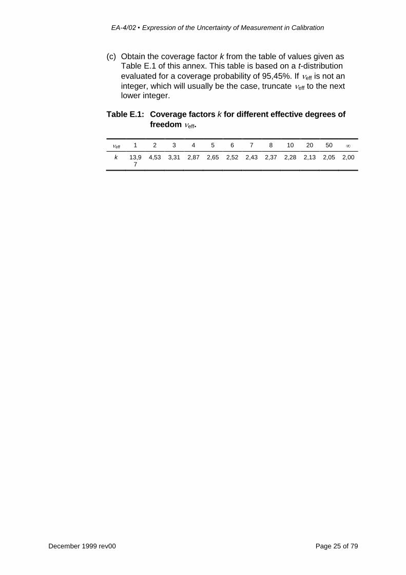
(c) Obtain the coverage factor k from the table of values given as Table E.1 of this annex. This table is based on a t-distribution

evaluated for a coverage probability of 95,45%. If eff is not an

integer, which will usually be the case, truncate eff to the next lower integer.

Table E.1: Coverage factors k for different effective degrees of

freedom eff.

eff 1 2 3 4 5 6 7 8 10 20 50

k 13,97

4,53 3,31 2,87 2,65 2,52 2,43 2,37 2,28 2,13 2,05 2,00



SUPPLEMENT 1

Examples



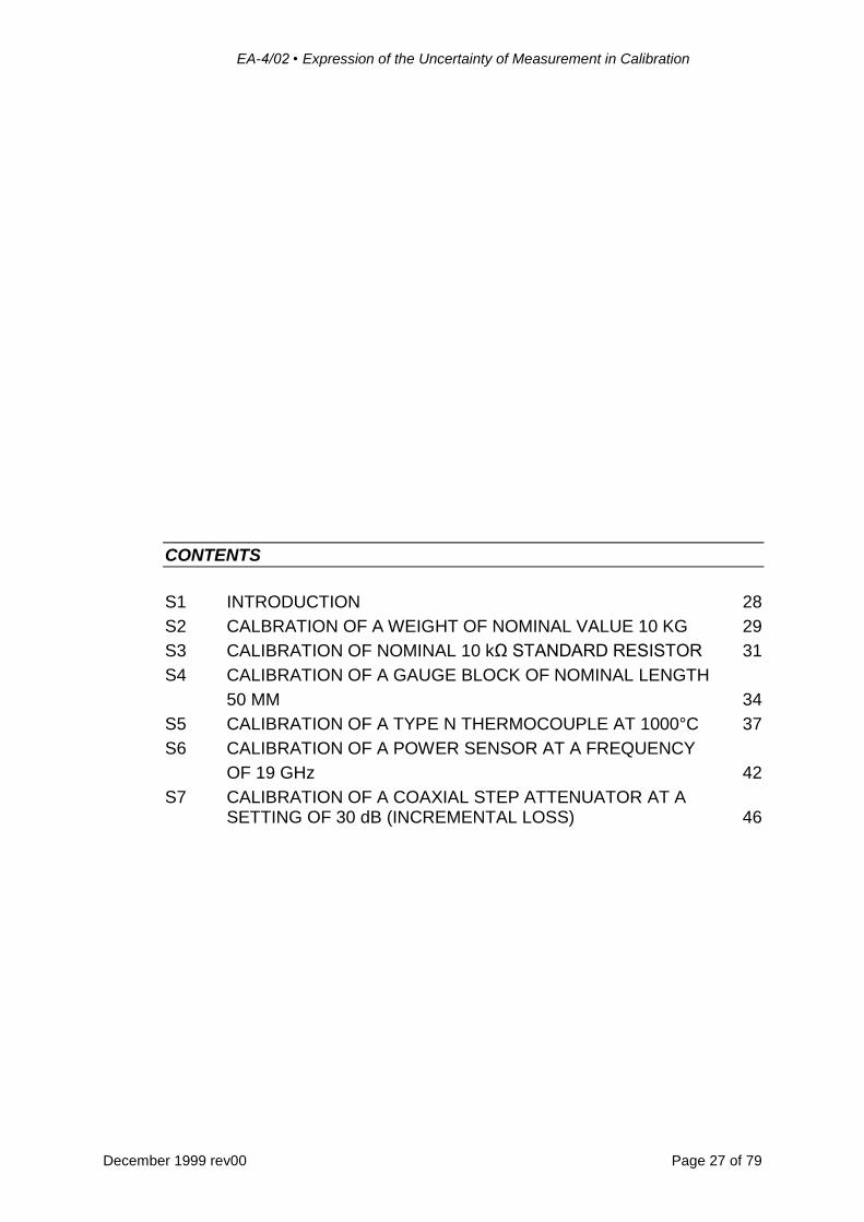
CONTENTS

S1 INTRODUCTION 28

S2 CALBRATION OF A WEIGHT OF NOMINAL VALUE 10 KG 29

S3 CALIBRATION OF NOMINAL 10 kΩ STANDARD RESISTOR 31

S4 CALIBRATION OF A GAUGE BLOCK OF NOMINAL LENGTH

50 MM 34

S5 CALIBRATION OF A TYPE N THERMOCOUPLE AT 1000°C 37

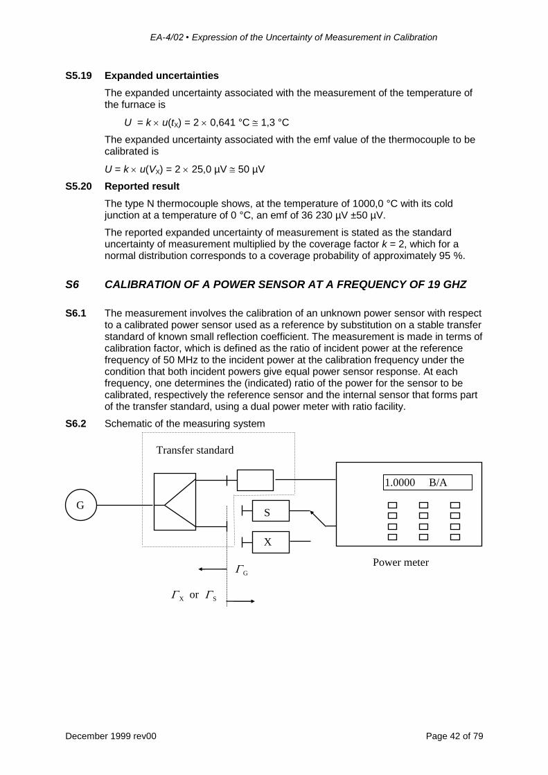
S6 CALIBRATION OF A POWER SENSOR AT A FREQUENCY

OF 19 GHz 42

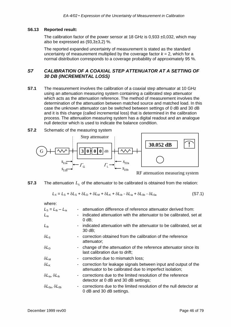
S7 CALIBRATION OF A COAXIAL STEP ATTENUATOR AT A SETTING OF 30 dB (INCREMENTAL LOSS) 46



S1 INTRODUCTION

S1.1 The following examples are chosen to demonstrate the method of evaluating the uncertainty of measurement. More typical and representative examples based on appropriate models have to be developed by special working groups in the different areas. Nevertheless, the examples presented here provide a general guidance on how to proceed.

S1.2 The examples are based on drafts prepared by EAL Expert Groups. These drafts have been simplified and harmonised to make them transparent to laboratory staff in all fields of calibration. It is thus hoped that this set of examples will contribute to a better understanding of the details of setting up the model of evaluation and to the harmonisation of the process of evaluating the uncertainty of measurement, independent of the field of calibration.

S1.3 The contributions and values given in the examples are not intended to imply mandatory or preferred requirements. Laboratories should determine the uncertainty contributions on the basis of the model function they use in the evaluation of the particular calibration they perform and report the evaluated uncertainty of measurement on the calibration certificate they issue. In all the examples given, the conditions stated in section 5 for the use of the standard coverage factor k = 2 are fulfilled.

S1.4 The presentation of the examples follows, in accordance with the step-by-step procedure of section 7 of EAL-R2, a common scheme containing:

a short descriptive title,

a general description of the process of measurement,

the model of evaluation with a list of symbols used,

an extended listing of input data with short descriptions of how they have been obtained,

the list of observations and the evaluation of the statistical parameters,

an uncertainty budget in table form,

the expanded uncertainty of measurement,

the reported complete result of measurement.

S1.5 This first supplement to EAL-R2 is intended to be followed by others containing further worked-out examples on the evaluation of uncertainty of measurement in connection with the calibration of instruments. Examples may also be found in EAL Guidance Documents dealing with the calibration of specific types of measurement instruments.



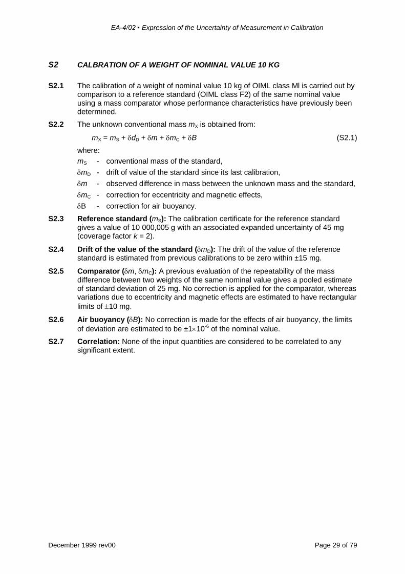
S2 CALBRATION OF A WEIGHT OF NOMINAL VALUE 10 KG

S2.1 The calibration of a weight of nominal value 10 kg of OIML class Ml is carried out by comparison to a reference standard (OIML class F2) of the same nominal value using a mass comparator whose performance characteristics have previously been determined.

S2.2 The unknown conventional mass mX is obtained from:

mX = mS + dD + m + mC + B (S2.1)

where:

mS - conventional mass of the standard,

mD - drift of value of the standard since its last calibration,

m - observed difference in mass between the unknown mass and the standard,

mC - correction for eccentricity and magnetic effects,

B - correction for air buoyancy.

S2.3 Reference standard (mS): The calibration certificate for the reference standard gives a value of 10 000,005 g with an associated expanded uncertainty of 45 mg (coverage factor k = 2).

S2.4 Drift of the value of the standard (mD): The drift of the value of the reference standard is estimated from previous calibrations to be zero within ±15 mg.

S2.5 Comparator (m, mC): A previous evaluation of the repeatability of the mass difference between two weights of the same nominal value gives a pooled estimate of standard deviation of 25 mg. No correction is applied for the comparator, whereas variations due to eccentricity and magnetic effects are estimated to have rectangular

limits of 10 mg.

S2.6 Air buoyancy (B): No correction is made for the effects of air buoyancy, the limits

of deviation are estimated to be ±110-6 of the nominal value.

S2.7 Correlation: None of the input quantities are considered to be correlated to any significant extent.



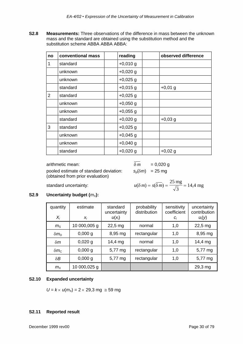
S2.8 Measurements: Three observations of the difference in mass between the unknown mass and the standard are obtained using the substitution method and the substitution scheme ABBA ABBA ABBA:

no conventional mass reading observed difference

1 standard +0,010 g

unknown +0,020 g

unknown +0,025 g

standard +0,015 g +0,01 g

2 standard +0,025 g

unknown +0,050 g

unknown +0,055 g


3 standard +0,025 g

unknown +0,045 g

unknown +0,040 g


arithmetic mean: m = 0,020 g

pooled estimate of standard deviation: sp(m) = 25 mg (obtained from prior evaluation)

standard uncertainty: u m s m( ) ( ) , 25

314 4

mgmg

S2.9 Uncertainty budget (mX):

quantity

Xi

estimate

xi

standard uncertainty

u(xi)

probability distribution

sensitivity coefficient

ci

uncertainty contribution

ui(y)

mS 10 000,005 g 22,5 mg normal 1,0 22,5 mg

mD 0,000 g 8,95 mg rectangular 1,0 8,95 mg

m 0,020 g 14,4 mg normal 1,0 14,4 mg

mC 0,000 g 5,77 mg rectangular 1,0 5,77 mg

B 0,000 g 5,77 mg rectangular 1,0 5,77 mg

mX 10 000,025 g 29,3 mg

S2.10 Expanded uncertainty

U = k u(mX) = 2 29,3 mg 59 mg

S2.11 Reported result



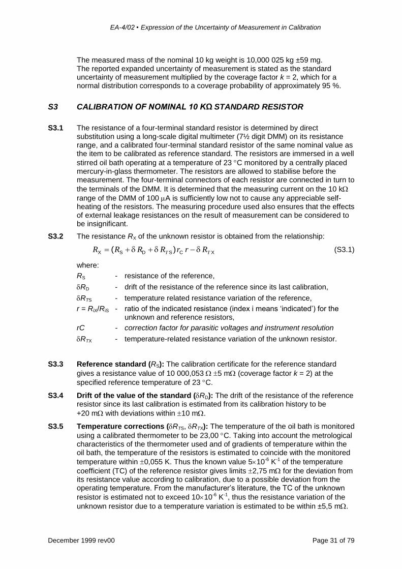
The measured mass of the nominal 10 kg weight is 10,000 025 kg ±59 mg. The reported expanded uncertainty of measurement is stated as the standard uncertainty of measurement multiplied by the coverage factor k = 2, which for a normal distribution corresponds to a coverage probability of approximately 95 %.

S3 CALIBRATION OF NOMINAL 10 KΩ STANDARD RESISTOR

S3.1 The resistance of a four-terminal standard resistor is determined by direct substitution using a long-scale digital multimeter (7½ digit DMM) on its resistance range, and a calibrated four-terminal standard resistor of the same nominal value as the item to be calibrated as reference standard. The resistors are immersed in a well

stirred oil bath operating at a temperature of 23 C monitored by a centrally placed mercury-in-glass thermometer. The resistors are allowed to stabilise before the measurement. The four-terminal connectors of each resistor are connected in turn to

the terminals of the DMM. It is determined that the measuring current on the 10 k

range of the DMM of 100 A is sufficiently low not to cause any appreciable self-heating of the resistors. The measuring procedure used also ensures that the effects of external leakage resistances on the result of measurement can be considered to be insignificant.

S3.2 The resistance RX of the unknown resistor is obtained from the relationship:

R R R R r r RT TX S D S C X( ) (S3.1)

where:

RS - resistance of the reference,

RD - drift of the resistance of the reference since its last calibration,

RTS - temperature related resistance variation of the reference,

r = RiX/RiS - ratio of the indicated resistance (index i means ‘indicated’) for the unknown and reference resistors,

rC - correction factor for parasitic voltages and instrument resolution

RTX - temperature-related resistance variation of the unknown resistor.

S3.3 Reference standard (RS): The calibration certificate for the reference standard

gives a resistance value of 10 000,053 5 m (coverage factor k = 2) at the

specified reference temperature of 23 C.

S3.4 Drift of the value of the standard (RD): The drift of the resistance of the reference resistor since its last calibration is estimated from its calibration history to be

+20 m with deviations within 10 m.

S3.5 Temperature corrections (RTS, RTX): The temperature of the oil bath is monitored

using a calibrated thermometer to be 23,00 C. Taking into account the metrological characteristics of the thermometer used and of gradients of temperature within the oil bath, the temperature of the resistors is estimated to coincide with the monitored

temperature within 0,055 K. Thus the known value 510-6 K-1 of the temperature

coefficient (TC) of the reference resistor gives limits 2,75 m for the deviation from its resistance value according to calibration, due to a possible deviation from the operating temperature. From the manufacturer’s literature, the TC of the unknown

resistor is estimated not to exceed 1010-6 K-1, thus the resistance variation of the

unknown resistor due to a temperature variation is estimated to be within ±5,5 m.



S3.6 Resistance measurements (rC): Since the same DMM is used to observe both RiX and RiS the uncertainty contributions are correlated but the effect is to reduce the uncertainty and it is only necessary to consider the relative difference in the resistance readings due to systematic effects such as parasitic voltages and instrument resolution (see the mathematical note in paragraph S3.12), which are

estimated to have limits of ±0,510-6 for each reading. The distribution resulting for

the ratio rC is triangular with expectation 1,000 000 0 and limits ±1,010-6.


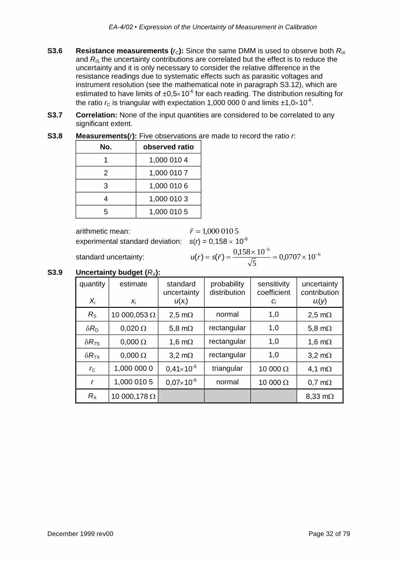
S3.8 Measurements(r): Five observations are made to record the ratio r:

No. observed ratio

1 1,000 010 4

2 1,000 010 7

3 1,000 010 6

4 1,000 010 3

5 1,000 010 5

arithmetic mean: r 1000 010 5,

experimental standard deviation: s(r) = 0,158 10-6

standard uncertainty: u r s r( ) ( )

0158 10

50 0707 10

66,

,

S3.9 Uncertainty budget (RX):

quantity

Xi

estimate

xi


u(xi)



ci


ui(y)

RS 10 000,053 2,5 m normal 1,0 2,5 m

RD 0,020 5,8 m rectangular 1,0 5,8 m

RTS 0,000 1,6 m rectangular 1,0 1,6 m

RTX 0,000 3,2 m rectangular 1,0 3,2 m

rC 1,000 000 0 0,4110-6 triangular 10 000 4,1 m

r 1,000 010 5 0,0710-6 normal 10 000 0,7 m

RX 10 000,178 8,33 m



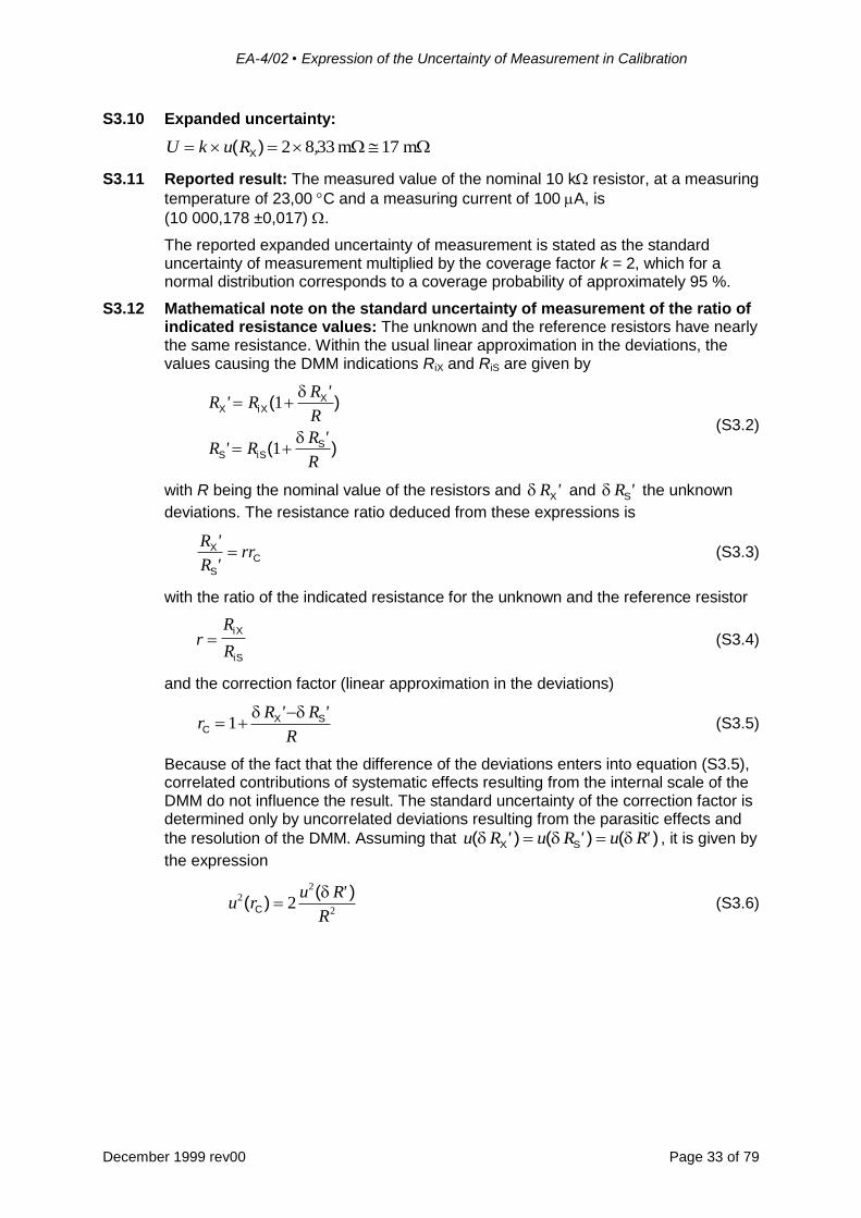
S3.10 Expanded uncertainty:

U k u R ( )X 2 8 33 17, m m

S3.11 Reported result: The measured value of the nominal 10 k resistor, at a measuring

temperature of 23,00 C and a measuring current of 100 A, is

(10 000,178 ±0,017) .

The reported expanded uncertainty of measurement is stated as the standard uncertainty of measurement multiplied by the coverage factor k = 2, which for a normal distribution corresponds to a coverage probability of approximately 95 %.

S3.12 Mathematical note on the standard uncertainty of measurement of the ratio of indicated resistance values: The unknown and the reference resistors have nearly the same resistance. Within the usual linear approximation in the deviations, the values causing the DMM indications RiX and RiS are given by

R RR

R

R RR

R

X iXX

S iSS

( )

( )

''

''

1

1

(S3.2)

with R being the nominal value of the resistors and RX' and RS' the unknown

deviations. The resistance ratio deduced from these expressions is

R

RrrX

S

C

'

' (S3.3)

with the ratio of the indicated resistance for the unknown and the reference resistor

rR

R

iX

iS

(S3.4)

and the correction factor (linear approximation in the deviations)

rR R

RC

X S

1 ' '

(S3.5)

Because of the fact that the difference of the deviations enters into equation (S3.5), correlated contributions of systematic effects resulting from the internal scale of the DMM do not influence the result. The standard uncertainty of the correction factor is determined only by uncorrelated deviations resulting from the parasitic effects and

the resolution of the DMM. Assuming that u R u R u R( ) ( ) ( )X S ' ' ' , it is given by

the expression

u ru R

R

22

22( )

( )C

' (S3.6)



S4 CALIBRATION OF A GAUGE BLOCK OF NOMINAL LENGTH 50 MM

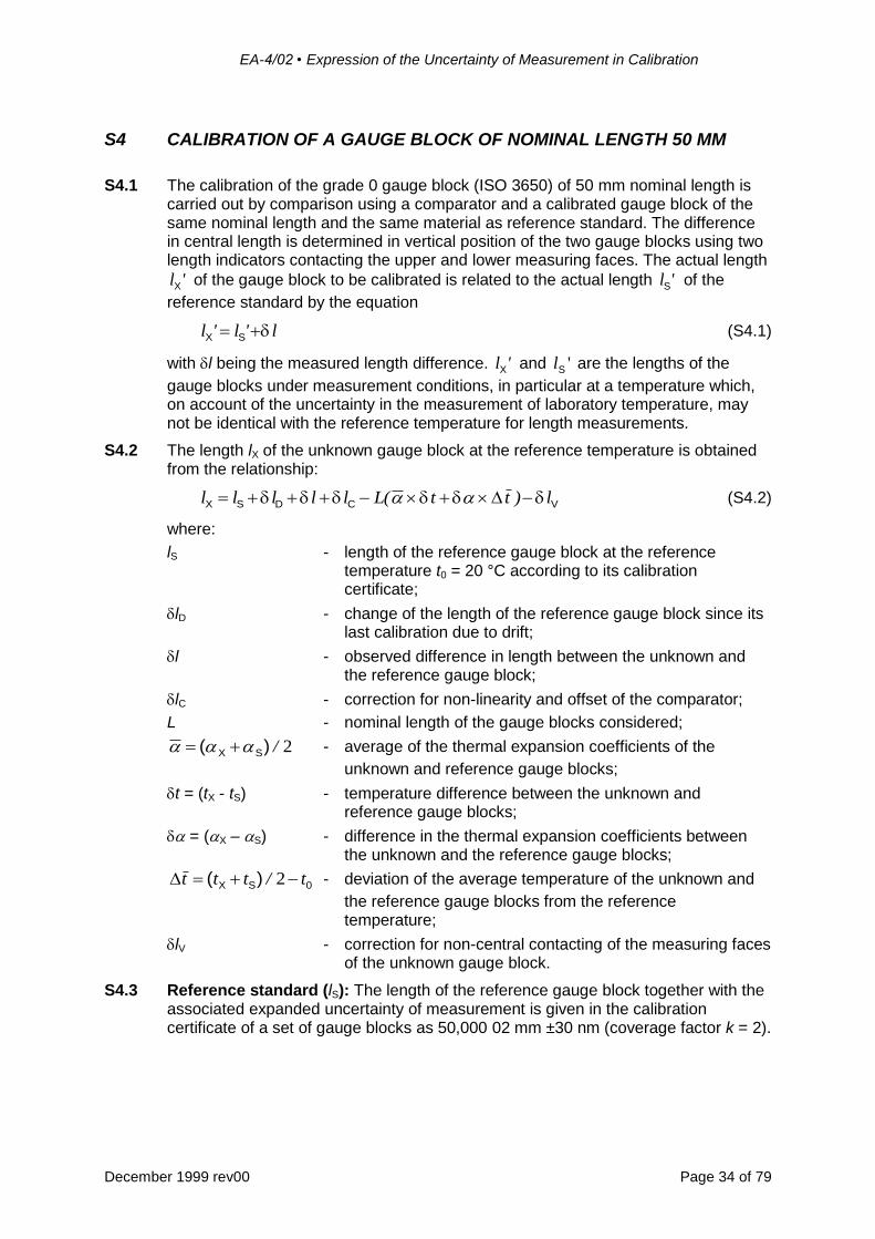
S4.1 The calibration of the grade 0 gauge block (ISO 3650) of 50 mm nominal length is carried out by comparison using a comparator and a calibrated gauge block of the same nominal length and the same material as reference standard. The difference in central length is determined in vertical position of the two gauge blocks using two length indicators contacting the upper and lower measuring faces. The actual length

lX' of the gauge block to be calibrated is related to the actual length lS' of the

reference standard by the equation

l l lX S' ' (S4.1)

with l being the measured length difference. lX' and lS ' are the lengths of the

gauge blocks under measurement conditions, in particular at a temperature which, on account of the uncertainty in the measurement of laboratory temperature, may not be identical with the reference temperature for length measurements.

S4.2 The length lX of the unknown gauge block at the reference temperature is obtained from the relationship:

l l l l l L t t lX S D C V ( ) (S4.2)

where:

lS - length of the reference gauge block at the reference temperature t0 = 20 °C according to its calibration certificate;

lD - change of the length of the reference gauge block since its last calibration due to drift;

l - observed difference in length between the unknown and the reference gauge block;

lC - correction for non-linearity and offset of the comparator;

L - nominal length of the gauge blocks considered;

( )X S / 2 - average of the thermal expansion coefficients of the

unknown and reference gauge blocks;

t = (tX - tS) - temperature difference between the unknown and reference gauge blocks;

= (X – S) - difference in the thermal expansion coefficients between the unknown and the reference gauge blocks;

t t t t ( ) 0X S / 2 - deviation of the average temperature of the unknown and

the reference gauge blocks from the reference temperature;

lV - correction for non-central contacting of the measuring faces of the unknown gauge block.

S4.3 Reference standard (lS): The length of the reference gauge block together with the associated expanded uncertainty of measurement is given in the calibration certificate of a set of gauge blocks as 50,000 02 mm ±30 nm (coverage factor k = 2).



S4.4 Drift of the standard (lD): The temporal drift of the length of the reference gauge block is estimated from previous calibrations to be zero with limits ±30 nm. General experience with gauge blocks of this type suggests that zero drift is most probable and that a triangular probability distribution can be assumed.

S4.5 Comparator (lC): The comparator has been verified to meet the specifications stated in EAL-G21. From this, it can be ascertained that for length differences D up

to ±10 m corrections to the indicated length difference are within the limits (30 nm

+0,02·D). Taking into account the tolerances of the grade 0 gauge block to be calibrated and the grade K reference gauge block, the maximum length difference

will be within ±1 m leading to limits of ±32 nm for non-linearity and offset corrections of the comparator used.

S4.6 Temperature corrections ( , t, , t ): Before calibration, care is taken to

ensure that the gauge blocks assume ambient temperature of the measuring room. The remaining difference in temperature between the standard and the gauge block to be calibrated is estimated to be within ±0,05 K. Based on the calibration certificate of the reference gauge block and the manufacturer’s data for the gauge block to be calibrated the linear thermal expansion coefficient of the steel gauge blocks is

assumed to be within the interval (11,5±1,0)10-6 C-1. Combining the two rectangular distributions the difference in linear thermal expansion coefficient is

triangularly distributed within the limits ±210-6 C-1. The deviation of the mean temperature of measurement from the reference temperature t0 = 20 °C is estimated

to be within ±0,5 C. The best estimates of the difference in linear expansion coefficients and the deviations of the mean temperature from the reference temperature are zero. Therefore second order terms have to be taken into account in the evaluation of their uncertainty contribution resulting in the product of standard

uncertainties associated with the factors of the product term t in equation

(S4.2) (see the mathematical note in paragraph S4.13, eq. (S4.5)). The final

standard uncertainty is u t( ) 0 236 10 6, .

S4.7 Variation in length (lV): For gauge blocks of grade 0 the variation in length determined from measurements at the centre and the four corners has to be within

±0,12 m (ISO 3650). Assuming that this variation occurs on the measuring faces along the short edge of length 9 mm and that the central length is measured inside a circle of radius 0,5 mm, the correction due to central misalignment of the contacting point is estimated to be within ±6,7 nm.




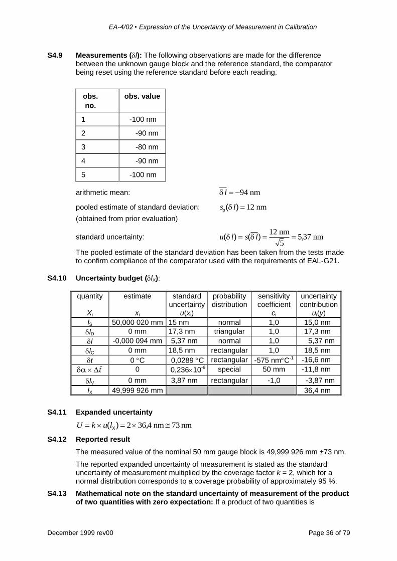
S4.9 Measurements (l): The following observations are made for the difference between the unknown gauge block and the reference standard, the comparator being reset using the reference standard before each reading.

obs.

no.

obs. value

1 -100 nm

2 -90 nm

3 -80 nm

4 -90 nm

5 -100 nm

arithmetic mean: l 94 nm

pooled estimate of standard deviation: s lp( ) 12 nm

(obtained from prior evaluation)

standard uncertainty: u l s l( ) ( ) 12

55 37

nmnm,

The pooled estimate of the standard deviation has been taken from the tests made to confirm compliance of the comparator used with the requirements of EAL-G21.

S4.10 Uncertainty budget (lX):

quantity

Xi

estimate

xi


u(xi)



ci


ui(y)

lS 50,000 020 mm 15 nm normal 1,0 15,0 nm

lD 0 mm 17,3 nm triangular 1,0 17,3 nm

l -0,000 094 mm 5,37 nm normal 1,0 5,37 nm

lC 0 mm 18,5 nm rectangular 1,0 18,5 nm

t 0 C 0,0289 C rectangular -575 nmC-1 -16,6 nm

t 0 0,23610-6 special 50 mm -11,8 nm

lV 0 mm 3,87 nm rectangular -1,0 -3,87 nm

lX 49,999 926 mm 36,4 nm


U k u l ( )X 2 36 4 73, nm nm


The measured value of the nominal 50 mm gauge block is 49,999 926 mm ±73 nm.


S4.13 Mathematical note on the standard uncertainty of measurement of the product of two quantities with zero expectation: If a product of two quantities is



considered, the usual method of evaluation of uncertainty contributions based on the linearisation of the model function has to be modified if one or both of the expectations of the factors in the product are zero. If the factors in the product are statistically independent with non-zero expectations, the square of the relative standard uncertainty of measurement (relative variance) associated with the product can be expressed without any linearisation by the squares of the relative standard uncertainties associated with the estimates of the factors:

w x x w x w x w x w x2

1 2

2

1

2

2

2

1

2

2( ) ( ) ( ) ( ) ( ) (S4.2)

Using the definition of the relative standard uncertainty of measurement this expression is easily transformed into the general relation

u x x x u x x u x u x u x2

1 2 2

2 2

1 1

2 2

2

2

1

2

2( ) ( ) ( ) ( ) ( ) (S4.3)

If the standard uncertainties u(x1) and u(x2) associated with the expectations x1 and x2 are much smaller than the moduli of the respective expectation values the third term on the right side may be neglected. The resulting equation represents the case described by the usual method based on the linearisation of the model function.

If, however, one of the moduli of the expectation values, for example x2, is much smaller than the standard uncertainty u(x2) associated with this expectation or even zero, the product term involving this expectation may be neglected on the right side of equation (S4.3), but not the third term. The resulting equation is

u x x x u x u x u x2

1 2 1

2 2

2

2

1

2

2( ) ( ) ( ) ( ) (S4.4)

If both moduli of the expectation values are much smaller than their associated standard uncertainties or even zero, only the third term in equation (S4.3) gives a significant contribution:

u x x u x u x2

1 2

2

1

2

2( ) ( ) ( ) (S4.5)

S5 CALIBRATION OF A TYPE N THERMOCOUPLE AT 1000°C

S5.1 A type N thermocouple is calibrated by comparison with two reference thermocouples of type R in a horizontal furnace at a temperature of 1000 °C. The emfs generated by the thermocouples are measured using a digital voltmeter through a selector/reversing switch. All thermocouples have their reference junctions at 0 °C. The thermocouple to be calibrated is connected to the reference point using compensating cables. Temperature values are give in the t90 temperature scale.

S5.2 The temperature tX of the hot junction of the thermocouple to be calibrated is

t t V V V Vt

Ct t

t V C V C V C VC

Ct t t

X S iS iS1 iS2 RS

S

D F

S iS S iS1 S iS2 S RS

S

S D F

( )

( )

0

0

0

0

(S5.1)



S5.3 The voltage VX across the thermocouple wires with the cold junction at 0 °C during calibration is

V t V tt

C

t

C

V V V V Vt

C

t

C

X X X

X

X

X

iX iX1 iX2 R LX

X

X

X

( ) ( )

0

0

0

0

(S5.2)

where:

tS(V) - temperature of the reference thermometer in terms of voltage with cold junction at 0 °C. The function is given in the calibration certificate;

ViS, ViX - indication of the voltmeter;

ViS1, ViX1 - voltage corrections obtained from the calibration of the voltmeter;

ViS2, ViX2 - voltage corrections due to the limited resolution of the voltmeter;

VR - voltage correction due to contact effects of the reversing switch;

t0S, t0X - temperature corrections due to the deviation of the reference

temperatures from 0 C;

CS, CX - sensitivities of the thermocouples for voltage at the measuring temperature of 1000 °C;

CS0, CX0 - sensitivities of the thermocouples for voltage at the reference

temperature of 0 C;

tD - change of the values of the reference thermometers since their last calibration due to drift;

tF - temperature correction due to non-uniformity of the temperature of the furnace;

t - temperature at which the thermocouple is to be calibrated (calibration point);

t = t - tX - deviation of the temperature of the calibration point from the temperature of the furnace;

VLX - voltage correction due to the compensating cables.

S5.4 The reported result is the output emf of the thermocouple at the temperature of its hot junction. Because the measurement process consists of two steps — determination of the temperature of the furnace and determination of emf of the thermocouple to be calibrated — the evaluation of the uncertainty of measurement is split in two parts.

S5.5 Reference standards (tS(V)): The reference thermocouples are supplied with calibration certificates that relate the temperature at their hot junction with their cold junction at 0 °C to the voltage across their wires. The expanded uncertainty of measurement at 1000 °C is U = 0,3 °C (coverage factor k = 2).



S5.6 Calibration of the voltmeter (ViS1, ViX1): The voltmeter has been calibrated. Corrections to the measured voltages are made to all results. The calibration certificate gives a constant expanded uncertainty of measurement for voltages smaller than 50 mV of U = 2,0 µV (coverage factor k = 2).

S5.7 Resolution of the voltmeter (ViS2, ViX2): A 4½ digit microvoltmeter has been used

in its 10 mV range resulting in resolution limits of ±0,5 V at each indication.

S5.8 Parasitic voltages (VR): Residual parasitic offset voltages due to the switch contacts have been estimated to be zero within ±2 µV.

S5.9 Reference temperatures (t0S, t0X): The temperature of the reference point of each thermocouple is known to be 0 °C within ±0,1 °C.

S5.10 Voltage sensitivities (CS, CX, CS0, CX0): The voltage sensitivities of the thermocouples have been taken from reference tables:

1000 °C 0 °C

reference thermocouple CS = 0,077 °C/µV CS0 = 0,189 °C/µV

unknown thermocouple CX = 0,026 °C/µV CS0 = 0,039 °C/µV

S5.11 Drift of the reference standard (tD): From previous calibrations the drift of the reference standards are estimated to be zero within the limits ±0,3 °C.

S5.12 Temperature gradients (tF): The temperature gradients inside the furnace have been measured. At 1000 °C, deviations from non-uniformity of temperature in the region of measurement are within ±1 °C.

S5.13 Compensating cables (VLX): The compensating cables have been investigated in

the range 0 C to 40 °C. From this, the voltage differences between the cables and the thermocouple wires are estimated to be within ±5 µV.

S5.14 Measurements (ViS, tS(ViS), ViX): The indications of the voltmeter are recorded in the following operational procedure which gives four readings for every thermocouple and reduces the effects of temperature drift in the thermal source and of parasitic thermal voltages in the measuring circuit:

1st cycle:

1st standard, unknown thermocouple, 2nd standard,

2nd standard, unknown thermocouple, 1st standard.

Reversion of polarity.

2nd cycle:

1st standard, unknown thermocouple, 2nd standard,

2nd standard, unknown thermocouple, 1st standard.



S5.15 The procedure requires that the difference between the two reference standards must not exceed ±0,3 °C. If the difference is not within these limits the observations have to be repeated and/or the reasons for such a large difference have to be investigated.

Thermocouple 1st reference Unknown 2nd reference

Indicated voltage, corrected +10500 µV +36245 µV +10503 µV

+10503 µV +36248 µV +10503 µV

-10503 µV -36248 µV -10505 µV

-10504 µV -36251 µV -10505 µV

Mean voltage 10502,5 µV 36248 µV 10504 µV

Temperature of the hot junction 1000,4 °C 1000,6 °C

Temperature of the furnace 1000,5 °C

S5.16 From the four readings on each thermocouple given in the table above, the mean value of the voltages of each thermocouple is deduced. The voltage values of the reference thermocouples are converted into temperature values by means of the temperature-voltage relations stated in their calibration certificates. The observed temperature values are highly correlated (correlation factor nearly one). Therefore, by taking their mean value, they are combined to one observation only, which is the temperature of the furnace at the location of the thermocouple to be calibrated. In a similar way, one observation of the voltage of the thermocouple to be calibrated has been extracted. In order to evaluate the uncertainty of measurement associated with these observations, a series of ten measurements has been previously undertaken at the same temperature of operation. It gave a pooled estimate of standard deviation for the temperature of the furnace and the voltage of the thermocouple to be calibrated.

The respective standard uncertainties of measurement of the observed quantities are:

pooled estimate of standard deviation: sp(tS) = 0,10 °C

standard uncertainty: u(tS) = s tp S( )

1 = 0,10 °C

pooled estimate of standard deviation: sp(ViX) = 1,6 µV

standard uncertainty: u(ViX) = s Vp iX( )

1= 1,6 µV



S5.17 Uncertainty budget (temperature tX of the furnace):

quantity

Xi

estimate

xi


u(xi)



ci


ui(y)

tS 1000,5 °C 0,10 °C normal 1,0 0,10 °C

ViS1 0 µV 1,00 µV normal 0,077 °C/µV 0,077 °C

ViS2 0 µV 0,29 µV rectangular 0,077 °C/µV 0,022 °C

VR 0 µV 1,15 µV rectangular 0,077 °C/µV 0,089 °C

t0S 0 °C 0,058 °C rectangular -0,407 -0,024 °C

tS 0 °C 0,15 °C normal 1,0 0,15 °C

tD 0 °C 0,173 °C rectangular 1,0 0,173 °C

tF 0 °C 0,577 °C rectangular 1,0 0,577 °C

tX 1000,5 °C 0,641 °C

S5.18 Uncertainty budget (emf VX of the thermocouple to be calibrated):

The standard uncertainty of measurement associated with the temperature deviation of the calibration point from the temperature of the furnace is the standard uncertainty of measurement associated with the temperature of the furnace because the temperature point is a defined value (exactly known).

quantity

Xi

estimate

xi


u(xi)



ci


ui(y)

ViX 36 248 µV 1,60 µV normal 1,0 1,60 µV

ViX1 0 µV 1,00 µV normal 1,0 1,00 µV

ViX2 0 µV 0,29 µV rectangular 1,0 0,29 µV

VR 0 µV 1,15 µV rectangular 1,0 1,15 µV

VLX 0 µV 2,9 µV rectangular 1,0 2,9 µV

t 0,5 °C 0,641 °C normal 38,5 µV/°C 24,5 µV

t0X 0 °C 0,058 °C rectangular -25,6 µV/°C -1,48 µV

VX 36 229 µV 25,0 µV



S5.19 Expanded uncertainties

The expanded uncertainty associated with the measurement of the temperature of the furnace is

U = k u(tX) = 2 0,641 °C 1,3 °C

The expanded uncertainty associated with the emf value of the thermocouple to be calibrated is

U = k u(VX) = 2 25,0 µV 50 µV


The type N thermocouple shows, at the temperature of 1000,0 °C with its cold junction at a temperature of 0 °C, an emf of 36 230 µV ±50 µV.


S6 CALIBRATION OF A POWER SENSOR AT A FREQUENCY OF 19 GHZ

S6.1 The measurement involves the calibration of an unknown power sensor with respect to a calibrated power sensor used as a reference by substitution on a stable transfer standard of known small reflection coefficient. The measurement is made in terms of calibration factor, which is defined as the ratio of incident power at the reference frequency of 50 MHz to the incident power at the calibration frequency under the condition that both incident powers give equal power sensor response. At each frequency, one determines the (indicated) ratio of the power for the sensor to be calibrated, respectively the reference sensor and the internal sensor that forms part of the transfer standard, using a dual power meter with ratio facility.

S6.2 Schematic of the measuring system

X

S

A

B

G

1.0000 B/A

G

S X

Power meter

Transfer standard

or



S6.3 The quantity K , termed ‘calibration factor’ by some manufacturers, is defined as:

KP

P

P

P

Ir

Ic

r Ar

c Ac

( )

( )

1

1

2

2

(S6.1)

for the equal power meter indication

where:

Pr - incident power at the reference frequency (50 MHz),

Pc - incident power at the calibration frequency,

r - voltage reflection coefficient of the sensor at the reference frequency

c - voltage reflection coefficient of the sensor at the calibration frequency

PAr - power absorbed by the sensor at the reference frequency

PAc - power absorbed by the sensor at the calibration frequency

S6.4 The calibration factor of the unknown sensor is obtained from the relationship

K K KM M

M Mp p p

r

X S D ( ) Sr Xc

Sc X

Cr Cc (S6.2)

where:

KS - calibration factor of the reference power sensor;

KD - change of the calibration factor of the reference power sensor since its last calibration due to drift;

MSr - mismatch factor of reference sensor at the reference frequency;

MSc - mismatch factor of standard sensor at the calibration frequency;

MXr - mismatch factor of sensor to be calibrated at the reference frequency;

MXc - mismatch factor of sensor to be calibrated at the calibration frequency;

pCr - correction of the observed ratio for non-linearity and limited resolution of the power meter at power ratio level of the reference frequency;

pCc - correction of the observed ratio for non-linearity and limited resolution of the power meter at power ratio level of the calibration frequency;

pp p

p p

Sr Xc

Sc Xr

- observed ratio of power ratios derived from:

pSr - indicated power ratio for the reference sensor at the reference frequency;

pSc - indicated power ratio for the reference sensor at the calibration frequency;

pXr - indicated power ratio for the sensor to be calibrated at the reference frequency;

pXc - indicated power ratio for the sensor to be calibrated at the calibration frequency.

S6.5 Reference sensor (KS): The reference sensor was calibrated six months before the calibration of the unknown power sensor. The value of the calibration factor, given in



the calibration certificate, is (95,7±1,1) % (coverage factor k = 2), which may also be expressed as 0,957±0,011.

S6.6 Drift of the standard (KD): The drift of the calibration factor of the reference standard is estimated from annual calibrations to be -0,002 per year with deviations within ±0,004. From these values, the drift of the reference sensor, which was calibrated half a year ago, is estimated to equal -0,001 with deviations within ±0,002.

S6.7 Linearity and resolution of the power meter (pCr, pCc): The expanded uncertainty of 0,002 (coverage factor k = 2) is assigned to the power meter readings at the power ratio level of the reference frequency and of 0,0002 (coverage factor k = 2) at the power ratio level of calibration frequency due to non-linearity of the power meter used. These values have been obtained from previous measurements. Since the same power meter has been used to observe both pS and pX, the uncertainty contributions at the reference as well at the calibration frequency are correlated. Because power ratios at both frequencies are considered, the effect of the correlations is to reduce the uncertainty. Thus, only the relative difference in the readings due to systematic effects should be taken into account (see the mathematical note in paragraph S3.12), resulting in a standard uncertainty of 0,00142 associated with the correction factor pCr and 0,000142 with the correction factor pCc.

The expanded uncertainty of measurement stated for the readings of the power meter contains linearity and resolution effects. The linearity effects are correlated whereas the resolution effects are uncorrelated. As shown in S3.12, building the power ratio cancels the influence of correlations and gives a reduced standard uncertainty of measurement to be associated with the ratio. In the calculations above, however, the separated correlated and uncorrelated contributions are not known and the values given are upper bounds for the standard uncertainty of measurement associated with ratios. The uncertainty budget finally shows that the contributions arising from these ratios are insignificant, i.e. the approximations are justified.

S6.8 Mismatch factors (MSr, MSc, MXr MXc): As the transfer standard system is not perfectly matched and the phase of the reflection coefficients of the transfer standard, the unknown and the standard power sensors are not known, there will be an uncertainty due to mismatch for each sensor at the reference frequency and at the calibration frequency. The corresponding limits of deviation have to be calculated for the reference and the calibration frequencies from the relationship:

MS,X G S,X 1 2 (S6.3)

where the magnitudes of the reflection coefficients of the transfer standard, the reference sensor and the sensor to be calibrated are:

50 MHz 18 GHz

G 0,02 0,07

S 0,02 0,10

X 0,02 0,12



The probability distribution of the individual contributions is U-shaped. This is taken into account by replacing the factor 1/3 for a rectangular distribution by 1/2 in calculating the variance from the square of the half-width determined from the limits. The standard uncertainty due to mismatch is therefore obtained from:

u M( )S,X

G S2

2

(S6.4)

Note: The values of the reflection coefficients are the results of measurements which are themselves subject to uncertainty. This is accounted for by adding the square root of the sum of the uncertainty of measurement squared and the measured value squared.


S6.10 Measurements (p): Three separate readings are made which involve disconnection and reconnection of both the reference sensor and the sensor to be calibrated on the transfer standard to take connector repeatability into account. The power meter readings used to calculate the observed power ratio p are as follows:

obs. no pSr pSc pXr pXc p

1 1,0001 0,9924 1,0001 0,9698 0,9772

2 1,0000 0,9942 1,0000 0,9615 0,9671

3 0,9999 0,9953 1,0001 0,9792 0,9836

arithmetic mean: p 0 976, 0

experimental standard deviation: s p( ) 0 0083,

standard uncertainty: u p s p( ) ( ) 0 0083

30 0048

,,

S6.11 Uncertainty budget (KX):

quantity

Xi

estimate

xi


u(xi)



ci


ui(y)

KS 0,957 0,0055 normal 0,976 0,00537

KD -0,001 0,0012 rectangular 0,976 0,00113

MSr 1,000 0,0006 U-shaped 0,933 0,00053

MSc 1,000 0,0099 U-shaped -0,933 0,00924

MXr 1,000 0,0006 U-shaped -0,933 -0,00053

MXc 1,000 0,0119 U-shaped 0,933 0,01110

pCr 1,000 0,0014 normal 0,933 0,00132

pCc 1,000 0,0001 normal 0,933 0,00013

p 0,976 0,0048 normal 0,956 0,00459

KX 0,933 0,01623


U = k u(KX) = 2 0,01623 0,032



S6.13 Reported result:

The calibration factor of the power sensor at 18 GHz is 0,933 ±0,032, which may also be expressed as (93,3±3,2) %.


S7 CALIBRATION OF A COAXIAL STEP ATTENUATOR AT A SETTING OF 30 DB (INCREMENTAL LOSS)

S7.1 The measurement involves the calibration of a coaxial step attenuator at 10 GHz using an attenuation measuring system containing a calibrated step attenuator which acts as the attenuation reference. The method of measurement involves the determination of the attenuation between matched source and matched load. In this case the unknown attenuator can be switched between settings of 0 dB and 30 dB and it is this change (called incremental loss) that is determined in the calibration process. The attenuation measuring system has a digital readout and an analogue null detector which is used to indicate the balance condition.

S7.2 Schematic of the measuring system

S7.3 The attenuation LX of the attenuator to be calibrated is obtained from the relation:

LX = LS + LS + LD + LM + LK + Lib - Lia + L0b - L0a (S7.1) where:

LS = Lib – Lia - attenuation difference of reference attenuator derived from:

Lia - indicated attenuation with the attenuator to be calibrated, set at 0 dB;

Lib - indicated attenuation with the attenuator to be calibrated, set at 30 dB;

LS - correction obtained from the calibration of the reference attenuator;

LD - change of the attenuation of the reference attenuator since its last calibration due to drift;

LM - correction due to mismatch loss;

LK - correction for leakage signals between input and output of the attenuator to be calibrated due to imperfect isolation;

Lia, Lib - corrections due to the limited resolution of the reference detector at 0 dB and 30 dB settings;

L0a, L0b - corrections due to the limited resolution of the null detector at 0 dB and 30 dB settings.

30.052 dB

dB 3 0 0 0 dB G

L G s22a s11a

s11b s22b RF attenuation measuring system

Step attenuator



S7.4 Reference attenuator (LS): The calibration certificate for the reference attenuator gives a value of attenuation for the 30,000 dB setting at 10 GHz of 30,003 dB with an associated expanded uncertainty of 0,005 dB (coverage factor k = 2). The correction of +0,003 dB with the associated expanded uncertainty of 0,005 dB (coverage factor k = 2) is considered to be valid for attenuation settings of the reference attenuator that differ not more than ±0,1 dB from the calibrated setting of 30,000 dB.

S7.5 Drift of the reference (LD): The drift of the attenuation of the reference attenuator is estimated from its calibration history to be zero with limits ±0,002 dB.

S7.6 Mismatch loss (LM): The reflection coefficients of the source and the load at the insertion point of the attenuator to be calibrated have been optimised by impedance matching to as low magnitudes as possible. Their magnitudes and the magnitudes of the scattering coefficients of the attenuator to be calibrated have been measured but their phase remains unknown. Without any phase information, a correction for mismatch error cannot be made, but the standard uncertainty (in dB) due to the incomplete knowledge of the match is estimated from the relationship [1]:

u L = s s s s s s( ) ( ) ( ) ( ) M S 11a 11b L 22a 22b S L 21a 21b

8 686

2

2 2 2 2 2 2 2 2 4 4,

(S7.2) with the source and load reflection coefficients

L = 0,03 and S = 0,03 and the scattering coefficients of the attenuator to be calibrated at 10 GHz

0 dB 30 dB

s11 0,05 0,09

s22 0,01 0,01

s21 0,95 0,031

as u(LM) = 0,02 dB. Note: The values of scattering and reflection coefficients are the results of

measurements which are themselves not exactly known. This is accounted for by adding the square root of the sum of uncertainty of measurement squared and the measured value squared.

S7.7 Leakage correction (LK): Leakage signals through the attenuator to be calibrated have been estimated from the measurements at 0 dB setting to be at least 100 dB below the measurement signal. The correction for leakage signals is estimated from these findings to be within ±0,003 dB at the 30 dB setting.

S7.8 Resolution of the reference attenuator setting (Lia, Lib): The digital readout of the reference attenuator has a resolution of 0,001 dB from which the correction for resolution is estimated to be within ±0,0005 dB.

S7.9 Resolution of the null detector (L0a, L0b): The detector resolution was determined from a previous evaluation to have a standard deviation of 0,002 dB at each reading with assumed normal probability distribution.




S7.11 Measurements (LS): Four observations are made of the incremental loss of the attenuator to be calibrated between settings of 0 dB and 30 dB:

obs. no. obs. values at

0 dB setting 30 dB setting

1 0,000 dB 30,033 dB

2 0,000 dB 30,058 dB

3 0,000 dB 30,018 dB

4 0,000 dB 30,052 dB

arithmetic mean: LS 30 040, dB

experimental standard deviation: s(LS) = 0,018 dB

standard uncertainty: u L s L( ) ( )S S 0 018

40 009

,,

dBdB

S7.12 Uncertainty budget (LX):

quantity

Xi

estimate

xi


u(xi)



ci


ui(y)

LS 30,040 dB 0,0090 dB normal 1,0 0,0090 dB

LS 0,003 dB 0,0025 dB rectangular 1,0 0,0025 dB

LD 0 dB 0,0011 dB U-shaped 1,0 0,0011 dB

LM 0 dB 0,0200 dB U-shaped 1,0 0,0200 dB

LK 0 dB 0,0017 dB U-shaped 1,0 0,0017 dB

Lia 0 dB 0,0003 dB U-shaped -1,0 -0,0003 dB

Lib 0 dB 0,0003 dB rectangular 1,0 0,0019 dB

L0a 0 dB 0,0020 dB rectangular -1,0 0,0020 dB

L0b 0 dB 0,0020 dB normal 1,0 -0,0020 dB

LX 30,043 dB 0,0224 dB


U = k u(LX) = 2 0,0224 dB 0,045 dB

S7.14 Reported result: The measured value of the step attenuator for a setting of 30 dB at 10 GHz is (30,043 ±0,045) dB. The reported expanded uncertainty of measurement is stated as the standard uncertainty of measurement multiplied by the coverage factor k = 2, which for a normal distribution corresponds to a coverage probability of approximately 95 %.

S7.15 Reference [1] Harris, I. A. ; Warner, F. L. : Re-examination of mismatch uncertainty when

measuring microwave power and attenuation. In: IEE Proc., Vol. 128, Pt. H, No. 1, Febr. 1981



SUPPLEMENT 2

Examples



CONTENTS

S8 INTRODUCTION 51

S9 CALBRATION OF A HAND-HELD DIGITAL MULTIMETER

AT 100 V DC 54

S10 CALIBRATION OF A VERNIER CALLIPER 58

S11 CALIBRATION OF A TEMPERATURE BLOCK CALIBRATOR

AT A TEMPERATURE OF 180°C 63

S12 CALIBRATION OF A HOUSEHOLD WATER METER 67

S13 CALIBRATION OF A RING GAUGE WITH A NOMINAL

DIAMETER OF 90 MM 71



S8 INTRODUCTION

S8.1 The following examples are chosen to demonstrate further the method of evaluating the uncertainty of measurement. They supplement the examples presented in Supplement 1 to EAL-R2 (Edition 1, November 1997). The present collection of examples focuses on situations where there are one or two dominant terms in the uncertainty propagation or where the number of repeated measurements is small.

S8.2 The examples are chosen to illustrate situations encountered in practice. It should be emphasised, however, that in practical applications there is no need to go through the mathematical derivations presented in these examples, in particular in the mathematical notes appended to some of the examples. Rather, the user is encouraged to employ the results of the theoretical presentations after having made himself acquainted with the conditions that have to be fulfilled. For instance, if it is ascertained, in a given situation, that the result of measurement has a rectangular distribution (as would be the case if there were only one term, rectangularly distributed, that needed to be considered in the propagation), one can immediately draw the conclusion that the coverage factor to be used to arrive at a coverage probability of 95 % is k = 1,65 (see S9.14).

S8.3 One general conclusion that may be drawn from the uncertainty propagation is that in the case of only one dominant contribution the type of distribution of this contribution applies for the result of measurement as well. However, to evaluate the uncertainty of the result of measurement, the applicable sensitivity coefficient has to be employed, as usual.

S8.4 It should be added that the situation where there is only one or a few dominant terms to the uncertainty of measurement is often met in connection with less complicated measuring instruments, where the dominant term often is due to the limited resolution of the instrument. Thus it may appear a paradox that the treatment of uncertainty of measurement for less complicated instruments, as shown by the examples of this Supplement, is more complicated than the treatment of the more straight-forward examples in Supplement 1. However, it should be kept in mind that the mathematical derivations, which may be felt as complications, are inserted for pedagogical reasons at places where they are needed instead of presenting them in the main document.

S8.5 The examples are based on drafts prepared by EA Expert Groups. These drafts have been simplified and harmonised to make them transparent to the laboratory staff in all fields of calibration. It is thus hoped that this set of examples, like the preceding set published as Supplement 1 to EAL-R2, will contribute to a better understanding of the details of setting up the model of evaluation and to the harmonisation of the process of evaluating the uncertainty of measurement, independent of the field of calibration.



S8.6 The contributions and values given in the examples are not intended to imply mandatory or preferred requirements. Laboratories should determine the uncertainty contributions on the basis of the model function they use in the evaluation of the particular calibration they perform and report the evaluated uncertainty of measurement on the calibration certificate they issue.

S8.7 The presentation of the examples follows the common scheme presented and implemented in the first supplement to EAL-R2. For details the reader is referred to clause S1.4 of that document.

S8.8 The uncertainty analysis of the examples is intended to represent the fundamentals of the specific measurement process and the method of evaluating the measurement result and the associated uncertainty. To keep the analysis transparent, also for those who are not experts in the relevant metrological field, a uniform method for the choice of the symbols of quantities has been followed, focused more on the physical background than on the current practice in different fields.

S8.9 There are several recurrent quantities involved in all cases. One of them is the mea-surand, i.e. the quantity to be measured, another is the quantity presented by the working standard, which realises the local unit; with this quantity the measurand is compared. Besides these two quantities there are several others, in all cases, which take the role of additional local quantities or corrections.

S8.10 Corrections describe the imperfect equality between a measurand and the result of a measurement. Some of the corrections are given by complete results of measurement, i.e. a measured value and its associated measurement uncertainty. For others the distribution of values is inferred from more or less complete knowledge of their nature. In most cases this will lead to an estimation of the limits for the unknown deviations.

S8.11 In certain cases the quantity presented by a working standard is characterised by the nominal value of the standard. Thus nominal values, which generally speaking characterise or identify calibration artefacts, often enter the uncertainty analysis.

S8.12 To distinguish in the mathematical models of evaluation between these concepts, the examples have been designed to follow the notational rules given below. It is evident, however, that it is not possible to follow such rules strictly, because the practice concerning the use of symbols is different in different metrological fields.

S8.13 The notation applied here distinguishes between main values, nominal values, correction values and values of limits: Main values are measured or observed values that contribute an essential part to the value of a measurand. They are represented by lower-case letters in italics; they will be preceded by an upper-case Greek delta if the quantity represents a difference.



EXAMPLE:

t i X - temperature indicated by a thermometer X to be calibrated. (index i means

indicated),

l - observed difference in the displacement of a measuring spindle.

Nominal values are assigned values of the realisation of a quantity by a standard or a measuring instrument. They are approximate values that give the main part of the realised value. They are represented by upper-case letters in italics. EXAMPLE: L - nominal length of a gauge block to be calibrated. Correction values give small deviations from the main values that are known or have to be estimated. In most cases they are additive. They are represented by the symbol chosen for the quantity under consideration, preceded by a lower-case Greek delta. EXAMPLE:

mD - possible deviation because of the drift of the value of a reference weight

since its last calibration

mC - correction for eccentricity of load and magnetic effects in the calibration of a

weight. Values of limits are fixed, estimated values of possible variations of the unknown values of a quantity. They are represented by the symbol chosen for the quantity under consideration, preceded by a upper-case Greek delta. EXAMPLE:

X - estimated half-width of the interval of possible deviations of a linear thermal

resistivity coefficient given in a manufacturer’s specification for a resistor to be calibrated.

The differentiation between different quantities of the same kind is effected by indices as shown in the examples. The internationally accepted notational rules for physical quantities have been followed: indices representing physical quantities are given in italics whereas indices that symbolise artefacts, instruments and so on are written in upright letters.

S8.14 Defined reference values are represented by a quantity symbol with the index zero. EXAMPLE:

p0 - reference pressure, e.g. of 1000 mbar.

S8.15 Ratios of quantities of the same kind (dimensionless ratios) are represented by

lower-case letters in italics.



EXAMPLE:

r R R i X i N/ - ratio of indicated resistance of an unknown resistor and a

reference resistor (index i means indicated).

S8.16 If several indices are used, the sequence of indices is chosen in such a way that the index representing the most general concept is leftmost and the one representing the most specific concept is rightmost. EXAMPLE:

Vi 1 ,Vi 2 - voltage indicated by voltmeter '1' and voltmeter '2', respectively

S8.17 The examples in this second supplement to EAL-R2 are intended to be followed by

others, illustrating different aspects encountered in connection with the calibration of measuring instruments. Examples may also be found in EAL and EA Guidance Documents1 dealing with the calibration of specific types of measuring instruments.

S9 CALBRATION OF A HAND-HELD DIGITAL MULTIMETER AT 100 V DC

S9.1 As part of a general calibration, a hand-held digital multimeter (DMM) is calibrated at an input of 100 V DC using a multifunction calibrator as a working standard. The following measuring procedure is used:

(1) The calibrator’s output terminals are connected to the input terminals of the DMM using suitable measuring wires.

(2) The calibrator is set to its 100V setting and, after a suitable stabilising period, the DMM reading is noted.

(3) The error of indication of the DMM is calculated using the DMM readings and the calibrator settings.

S9.2 It must be noted that the error of indication of the DMM which is obtained using this measuring procedure includes the effect of offset as well as deviations from linearity.

S9.3 The error of indication EX of the DMM to be calibrated is obtained from

SXiSXiX VVVVE (S9.1)

where

Vi X - voltage, indicated by the DMM (index i means indication),

VS - voltage generated by the calibrator,

XiV - correction of the indicated voltage due to the finite resolution of the DMM,

1 EAL-G26, Calibration of pressure balances

EAL-G31, Calibration of thermocouples

EAL-G32, Measurement and generation of small ac voltages with inductive voltage dividers

EA-10/10, EA Guidelines on the Determination of Pitch Diameter of Parallel Thread gauges by Mechanical

Probing



SV - correction of the calibrator voltage due to

(1) drift since its last calibration,

(2) deviations resulting from the combined effect of offset, non-linearity and differences in gain,

(3) deviations in the ambient temperature,

(4) deviations in mains power,

(5) loading effects resulting from the finite input resistance of the DMM to be calibrated.

S9.4 Because of the limited resolution of the indication of the DMM, no scatter in the

indicated values is observed.

S9.5 DMM readings ( XiV )

The DMM indicates the voltage 100,1 V at the calibrator setting 100 V. The DMM reading is assumed to be exact (see S9.4).

S9.6 Working standard ( SV )

The calibration certificate for the multifunction calibrator states that the voltage generated is the value indicated by the calibrator setting and that the associated expanded relative uncertainty of measurement is W=0,000 02 (coverage factor k 2), resulting in an expanded uncertainty of measurement associated with the 100 V setting of U=0,002 V (coverage factor k 2).

S9.7 Resolution of DMM to be calibrated ( XiV )

The least significant digit of the DMM display corresponds to 0,1 V. Each DMM reading has a correction due to the finite resolution of the display which is estimated to be 0,0 V with limits of +0.05 V (i.e. one half of the magnitude of the least significant digit).

S9.8 Other corrections ( SV )

Because of the fact that individual figures are not available the uncertainty of measurement associated with the different sources is derived from the accuracy specification given by the manufacturer of the calibrator. These specifications state that the voltage generated by the calibrator coincides with the calibrator setting

within (0,000 1VS +1 mV)2 under the measuring conditions

(1) the ambient temperature is within the range 18 C to 23 C

(2) the mains voltage powering the calibrator is in the range 210 V to 250 V,

(3) the resistive load at the calibrator’s terminals is greater than 100 k,

(4) the calibrator has been calibrated within the last year. Since these conditions of measurement are fulfilled and the calibration history of the calibrator shows that the manufacturer’s specification may be relied upon, the correction to be applied to the voltage generated by the calibrator is assumed to be

0,0 V within 0,011 V.

S9.9 Correlation

2 A widely used method of presenting accuracy specification of measuring instruments in data sheets or manuals

consists in giving the specification limits in terms of ‘settings’. For the calibrator, the statement would be

(0,01% of setting + 1 mV). Even if this method is considered to be equivalent to the expression given above it

is not used here because it may be misleading in many cases and because it does not represent an equation of

physical quantities in the internationally accepted symbolic nomenclature.



None of the input quantities are considered to be correlated to any significant extent.

S9.10 Uncertainty budget ( XE )

quantity

iX

estimate

ix


)( ixu



ic


)(yui

Vi X 100,1 V - - - -

VS 100,0 V 0,001 V normal -1,0 -0,001 V

XiV 0,0 V 0,029 V rectangular 1,0 0,029 V

SV 0,0 V 0,0064 V rectangular -1,0 -0,0064 V

EX 0,1 V 0,030 V


The standard uncertainty of measurement associated with the result is clearly dominated by the effect of the finite resolution of the DMM. The final distribution is not normal but essentially rectangular. Therefore, the method of effective degrees of freedom described in Annex E of EAL-R2 is not applicable. The coverage factor appropriate for a rectangular distribution is calculated from the relation given in eq. (S9.8) in the mathematical note S9.14.

V0,05V030,065,1)( XEukU

S9.12 Reported result The measured error of indication of the hand-held digital voltmeter at 100 V is

(0,10 0,05) V. The reported expanded uncertainty of measurement is stated as the standard

uncertainty of measurement multiplied by the coverage factor 65,1k which has

been derived from the assumed rectangular probability distribution for a coverage probability of 95%.

S9.13 Additional remark The method used for calculating the coverage factor is clearly related to the fact that the measurement uncertainty associated with the result is dominated by the effect of the finite resolution of the DMM. This will be true for the calibration of all low-resolution indicating instruments provided the finite resolution is the only dominant source in the uncertainty budget.



S9.14 Mathematical note If the situation of measurement is such that one of the uncertainty contributions in the budget can be identified as a dominant term, for instance the term with index 1, the standard uncertainty to be associated with the measurement result y can be

written as

)()()( 2

1 yuyuyu 2

R . (S9.2)

Here is

N

i

i yuyu2

2 )()(R (S9.3)

denotes the total uncertainty contribution of the non-dominant terms. As long as the

ratio of the total uncertainty contribution u yR ( ) of the non-dominant terms to the

uncertainty contribution u y1( ) of the dominant term is not larger than 0,3, eq. (S9.2)

may be approximated by

2

1

1)(

)(

2

11)()(

yu

yuyuyu R . (S9.4)

The relative error of approximation is smaller than 3101 . The maximum relative

change in the standard uncertainty resulting from the factor within the brackets in eq. (S9.4) is not larger than 5%. This value is within the accepted tolerance for mathematical rounding of uncertainty values. Under these assumptions the distribution of values that could reasonably be attributed to the measurand is essentially identical with the distribution resulting from the known dominant contribution. From this distribution density ( )y the coverage

probability p may be determined for any value of the expanded measurement

uncertainty U by the integral relation

Uy

Uy

dyyUp ')'()( . (S9.5)

Inverting this relation for a given coverage probability results in the relation between the expanded measurement uncertainty and the coverage probability U U p ( ) for

the given distribution density ( )y . Using this relation, the coverage factor may

finally be expressed as

)(

)()(

yu

pUpk . (S9.6)



In the case of the hand-held digital voltmeter the dominant uncertainty contribution

resulting from the finite resolution of the indication is V029,0)( XXEu V whereas

the total uncertainty contribution of the non-dominant terms is V0064,0)( XR Eu .

The relevant ratio is 22,0)(/)( XXR XEuEu V . Thus the resulting distribution of

values that can reasonably be attributed as errors of indications is essentially rectangular. The coverage probability for a rectangular distribution is linearly related to the expanded measurement uncertainty ( a being the half-width of the rectangular distribution)

a

Up . (S9.7)

Solving this relation for the expanded measurement uncertainty U and inserting the result together with the expression of the standard measurement uncertainty related to a rectangular distribution as given by eq. (3.8) of EAL-R2 finally gives the relation

3)( ppk . (S9.8)

For a coverage probability p 95 % applicable in the EA, the relevant coverage

factor is thus k 1 65, .

S10 CALIBRATION OF A VERNIER CALLIPER

S10.1 A vernier calliper made of steel is calibrated against grade I gauge blocks of steel used as working standards. The measurement range of the calliper is 150 mm. The reading interval of the calliper is 0,05 mm (the main scale interval is 1 mm and the vernier scale interval 1/20 mm). Several gauge blocks with nominal lengths in the range 0,5 - 150 mm are used in the calibration. They are selected in such a way that the measurement points are spaced at nearly equal distances (e.g. at 0 mm, 50 mm, 100 mm, 150 mm) but give different values on the vernier scale (e.g. 0,0 mm, 0,3 mm, 0,6 mm, 0,9 mm). The example concerns the 150 mm calibration point for measurement of external dimensions. Before calibration several checks of the condition of the calliper are made. These include dependence of the result of measurement on the distance of the measured item from the beam (Abbe error), quality of the measuring faces of the jaws (flatness, parallelism, squareness), and function of the locking mechanism.

S10.2 The error of indication XE of the calliper at the reference temperature t0 20 C is

obtained from the relation:

MXiSSXiX lltLllE (S10.1)

where:



Xil - indication of the calliper,

lS - length of the actual gauge block,

LS - nominal length of the actual gauge block,

- average thermal expansion coefficient of the calliper and the gauge block,

t - difference in temperature between the calliper and the gauge block,

Xil - correction due to the finite resolution of the calliper,

Ml - correction due to mechanical effects, such as applied measurement

force, Abbe errors, flatness and parallelism errors of the measurement faces.

S10.3 Working standards ( Sl , LS )

The lengths of the reference gauge blocks used as working standards, together with their associated expanded uncertainty of measurement, are given in the calibration certificate. This certificate confirms that the gauge blocks comply with the requirements for grade I gauge blocks according to ISO 3650, i.e. that the central length of the gauge blocks coincides within ±0,8 µm with the nominal length. For the actual lengths of the gauge blocks their nominal lengths are used without correction, taking the tolerance limits as the upper and lower limits of the interval of variability.

S10.4 Temperature (t , )

After an adequate stabilisation time, the temperatures of the calliper and the gauge block are equal within ±2 °C. The average thermal expansion coefficient is 11,5·10-6 °C-1. (The uncertainty in the average thermal expansion coefficient and in the difference of the thermal expansion coefficients has not been taken into account; its influence is considered negligible for the present case. Cf. EAL-R2-S1, example S4.)

S10.5 Resolution of the calliper ( Xil )

The scale interval of the vernier scale is 0,05 mm. Thus variations due to the finite

resolution are estimated to have rectangular limits of 25 µm.

S10.6 Mechanical effects ( Ml )

These effects include the applied measurement force, the Abbe error and the play between the beam and the sliding jaw. Additional effects may be caused by the fact that the measuring faces of the jaws are not exactly flat, not parallel to each other and not perpendicular to the beam. To minimise effort, only the range of the total variation, equal to ±50 µm is considered.

S10.7 Correlation None of the input quantities are considered to be correlated to any significant extent.

S10.8 Measurements ( Xil )

The measurement is repeated several times without detecting any scatter in the observations. Thus uncertainty due to limited repeatability does not give a contribution. The result of measurement for the 150 mm gauge block is 150,10 mm.



S10.9 Uncertainty budget ( lX )

quantity

X i

estimate

xi


u xi( )



ci


u yi ( )

Xil 150,10 mm - - - -

lS 150,00 m 0,46 µm rectangular -1,0 -0,46 µm

t 0 1,15 K rectangular 1,7 µMk-1 2,0 µm

Xil 0 15 µm rectangular 1,0 15 µm

Ml 0 29 µm rectangular 1,0 29 µm

XE 0,10 mm 33 µm


The uncertainty of measurement associated with the result is clearly dominated by the combined effect of the measurement force and the finite resolution of the vernier. The final distribution is not normal but essentially trapezoidal with a ratio

0 33, of the half-width of the plateau region to the half-width of the variability

interval. Therefore the method of effective degrees of freedom described in EAL-R2, Annex E is not applicable. The coverage factor k = 1,83 appropriate for this trapezoidal distribution of values is calculated from eq. (S10.10) of the mathematical note S10.13. Thus

mm06,0mm033,083,1)( XEukU


At 150 mm the error of indication of the calliper is (0,10 ± 0,06) mm. The reported expanded uncertainty of measurement is stated as the standard

uncertainty of measurement multiplied by the coverage factor k 183, which has

been derived from the assumed trapezoidal probability distribution for a coverage probability of 95 %.

S10.12 Additional remark The method used for calculating the coverage factor is clearly related to the fact that uncertainty of measurement associated with the result is dominated by two influences: the mechanical effects and the finite resolution of the vernier scale. Thus the assumption of a normal distribution for the output quantity is not justified and the conditions of EAL-R2, paragraph 5.6 apply. In the sense that probabilities and

probability densities in practice may only be determined to within 3 % 5 %, the distribution is essentially trapezoidal, obtained by convolution of the two rectangular distributions associated with the dominant contributions. The half-widths of the base

and the top of the resulting symmetrical trapezoid are 75 m and 25 m, respectively. 95 % of the area of the trapezoid is encompassed by an interval

60 m around its symmetry axis, corresponding to k 183, .

S10.13 Mathematical note

If the situation of measurement is such that two of the uncertainty contributions in the budget can be identified as dominant terms, the method presented in S9.14 can be applied when the two dominant contributions, for instance the terms with indices



1 and 2 , are combined into one dominant term. The standard uncertainty to be associated with the measurement result y may be written in this case as

u y u y u y( ) ( ) ( ) 0

2

R

2 (S10.2)

where

u y u y u y0( ) ( ) ( ) 1

2

2

2 (S10.3)

denotes the combined contribution of the two dominant terms and

u y u yii

N

R( ) ( )

2

3

(S10.4)

the total uncertainty contribution of the remaining non-dominant terms. If the two dominant contributions arise from rectangular distributions of values with half-widths

a1 and a2 , the distribution resulting from convolving them is a symmetrical

trapezoidal distribution

0

0,2

0,4

0,6

0,8

1

-2 -1 0 1 2

normalized deviation [y/a]

pro

bab

ilit

y d

en

sit

y [

p]

Fig. 1: Unified symmetrical trapezoidal probability distribution with the value

=0,33 of the edge parameter, resulting from the convolution of two rectangular distributions.



with half-widths

a a a 1 2 and b a a 1 2 (S10.5)

of the base and the top, respectively (see example in Fig. 1). The distribution may be conveniently expressed in the unified form

ya

ayaa

y

ay

ay

0

11

1

1

)1(

1)(

(S10.6)

with the edge parameter

b

a

a a

a a

1 2

1 2

(S10.7)

The square of the standard measurement uncertainty deduced from the trapezoidal distribution of eq. (S10.6) is

u ya

2

2

2

61( ) ( ) . (S10.8)

Using the distribution of eq. (S10.6) the dependence of the coverage factor on the coverage probability is derived according to the method sketched in S9.14

p

pp

p

pp

pk

2)1)(1(1

22

)1(

6

1

1)(

22

(S10.9)

Fig. 2 shows the dependence of the coverage factor k on the value of the edge

parameter for a coverage probability of 95 %.

1,5

1,6

1,7

1,8

1,9

2

0 0,2 0,4 0,6 0,8 1

edge parameter [beta]

co

vera

ge f

acto

r [k

]



Fig. 2: Dependence of the coverage factor k on the value of the edge parameter of a trapezoidal distribution for a coverage probability of 95 %.

The coverage factor for a coverage probability of 95 % appropriate to a trapezoidal

distribution with an edge parameter of 95,0 is calculated from the relation

6

1

)1)(1(1

2

2

pk . (S10.10)

S11 CALIBRATION OF A TEMPERATURE BLOCK CALIBRATOR AT A TEMPERATURE OF 180°C3

S11.1 As part of a calibration, the temperature that has to be assigned to the calibration bore of a temperature block calibrator, is measured. This is done when the indication of the built-in temperature indicator has stabilised at 180,0 °C. The temperature of the calibration bore is determined by an inserted platinum resistance thermometer, used as a working standard, by measuring the electrical resistance of

the thermometer by an ac resistance bridge. The temperature tX , that has to be

assigned as the temperature of the bore when the reading of the built-in temperature indicator is 180,0 °C, is given by:

VHARXiDSSX ttttttttt (S11.1)

3 A similar example will be found in the EA guideline EA-10/xx, Calibration of temperature block calibrators.

It has been included here, in a dimplified form, in order to highligt how a value is assigned to an indication of

an instrument in a calibration process. This process is basic for calibrations in different metrological fields

and, therefore, of general interest. The example further demonstrates that there are two equivalent ways to

tackle this problem: the direct assignment of a value to the indication of the instrument and the association of

a correction to the indication, usually called the error of indication.



where:

tS - temperature of the working standard derived from the ac resistance measurement,

tS - temperature correction due to the ac resistance measurement,

tD - temperature correction due to drift in the value of the working standard since its last calibration,

ti X - temperature correction due to the settability limitations of the block temperature calibrator,

Rt - temperature correction due to the radial temperature difference between the built-in thermometer and the working standard,

At - temperature correction due to the axial inhomogeneity of temperature in the measuring bore,

tH - temperature correction due to hysteresis in the increasing and decreasing branches of the measuring cycle,

tV - temperature variation within the time of measurement.

Temperature corrections due to stem conduction are not considered, since the platinum resistance thermometer used as working standard has an outer diameter

d 6 mm . Prior investigations have shown that stem conduction effects can be

neglected in this case.

S11.2 Working standard ( tS )

The calibration certificate of the resistance thermometer used as working standard gives the relationship between resistance and temperature. The measured resistance value corresponds to a temperature of 180,1 °C, with an associated

expanded uncertainty of measurement U = 30 mK (coverage factor k 2 ).

S11.3 Determination of the temperature by resistance measurement( tS )

The temperature of the resistance thermometer used as working standard is determined as 180,1 °C. The standard measurement uncertainty associated with the resistance measurement converted to temperature corresponds to

u t( ) S 10 mK .

S11.4 Drift of the temperature of the working standard ( tD )

From general experience with platinum resistance thermometers of the type used as working standard in the measurement, the change of temperature due to resistance ageing since the last calibration of the standard is estimated to be within the limits ±40 mK.

S11.5 Settability of the block temperature calibrator ( ti X )

The built-in controlling thermometer of the block temperature calibrator has a scale interval of 0,1 K. This gives temperature resolution limits of ±50 mK within which the thermodynamic state of the temperature block can be uniquely set. Note: If the indication of the built-in temperature indicator is not given in units of temperature the resolution limits must be converted into equivalent temperature values by multiplying the indication with the relevant instrument constant.



S11.6 Radial inhomogeneity of temperature ( Rt )

The radial temperature difference between the measuring bore and the built-in thermometer has been estimated to be within ±100 mK.

S11.7 Axial inhomogeneity of temperature ( At )

The temperature deviations due to axial inhomogeneity of temperature in the calibration bore have been estimated from readings for different immersion depths to be within ±250 mK.

S11.8 Hysteresis effects ( tH )

From readings of the reference thermometer during measurement cycles of increasing and decreasing temperature, the temperature deviation of the calibration bore due to hysteresis effect has been estimated to be within ±50 mK.

S11.9 Temperature instability ( tV )

Temperature variations due to temperature instability during the measuring cycle of

30 min are estimated to be within 30 mK.

S11.10 Correlations None of the input quantities are considered to be correlated to any significant extent.

S11.11 Repeated observations Due to the finite resolution of the indication of the built-in thermometer no scatter in the indicated values has been observed and taken into account.

S11.12 Uncertainty budget ( tX )

Quantity

X i

Estimate

xi

Standard uncertainty

u xi( )

Probability distribution

Sensitivity coefficient

ci

Uncertainty contribution

u yi ( )

tS 180,1 °C 15 mK normal 1,0 15 mK

tS 0,0 °C 10 mK normal 1,0 10 mK

tD 0,0 °C 23 mK rectangular 1,0 23 mK

ti X 0,0 °C 29 mK rectangular -1,0 -29 mK

Rt 0,0 °C 58 mK rectangular 1,0 58 mK

At 0,0 °C 144 mK rectangular 1,0 144 mK

tH 0,0 °C 29 mK rectangular 1,0 29 mK

tV 0,0 °C 17 mK rectangular 1,0 17 mK

tX 180,1 °C 164 mK



S11.13 Expanded uncertainty The standard uncertainty of measurement associated with the result is clearly dominated by the effect of the unknown temperature correction due to the axial temperature inhomogeneity in the measuring bore and the radial temperature difference between the built-in thermometer and the working standard. The final distribution is not normal but essentially trapezoidal. According to S10.13, the

coverage factor corresponding to the edge parameter 43,0 is 8,1k 1.

K3,0mK16481,1)( X tukU


The temperature of the calibration bore that has to be assigned to an indication of the built-in controlling thermometer of 180,0 °C is 180,1 °C ± 0,3 °C. The reported expanded uncertainty of measurement is stated as the standard

uncertainty of measurement multiplied by the coverage factor 81,1k which has

been derived from the assumed trapezoidal probability distribution for a coverage probability of 95 %.

S11.15 Mathematical note concerning the model Some metrologists are confused that the indication of the controlling thermometer does not appear explicitly in the model function of eq. (S11.1). To fit their needs, the problem can alternatively be formulated with the error of indication

iXX ttE (S11.2)

of the built-in temperature indicator

VHARXiDSiSX tttttttttE (S11.3)

The indicated value t i is a nominal value. Its effect is to shift the scale of the

measurand. It does, however, not contribute to the uncertainty of measurement associated with the error of indication

u E u t( ) ( )X X (S11.4)

The model function of eq. (S11.1) can be regained from eq. (S11.3) using the definition of the error of indication in eq. (S11.2). This note shows that there is not necessarily only one unique way to choose the model of evaluation of measurement. The metrologist keeps it in his hands to choose the model that suits his habits and his approach to the problem. Model functions that can be transformed mathematically from one into the other represent the same measurement process. For cases where a continuous scale of indication is involved, as in the calibration of the temperature block under consideration, model functions that are connected by linear scale transformations may serve as equivalent expressions of the measurement problem.



S12 CALIBRATION OF A HOUSEHOLD WATER METER

S12.1 The calibration of a water meter involves the determination of the relative error of indication within the applicable flow range of the meter. The measurement is made using a test rig that supplies necessary water flow with a pressure of approximately 500 kPa, a value typical for municipal tap water systems. The water is received in an open collecting tank that has been calibrated and determines the reference volume of the water. It is empty but wetted at the beginning of the measurement. The collecting tank has a narrow neck with an attached scale by which the filling level can be detected. The meter to be calibrated is connected between these tanks. It has a mechanical counter with pointers. The measurement is done at a flow rate of 2500 l/h with standing start-and-stop which means that the flow rate is zero both at the beginning and the end of the measurement. The indication of the meter is recorded at the beginning and at the end of the measurement. The level is recorded in the collecting tank at the end of the measurement. The temperature and pressure of the water at the meter, and the temperature of the water in the collecting tank, are recorded as well.

S12.2 The relative error of indication eX in a single run is defined as

1

X

X1iX2iXi

XV

VVVe

(S12.1)

with

)(1)(1)(1)( 0 SXWSXWSSSiSiX ppttttVVV (S12.2)

where: V V Vi X iX 2 iX 1 - difference in meter indications,

Vi X 1, Vi X 2 - indication of the meter at the beginning of the measurement and at the end of the measurement,

1XiV , 2XiV - corrections due to the finite resolution of the meter indication,

XV - volume that passed the meter during the measurement under the

prevailing conditions, i.e. pressure pX and temperature tX , at

the inlet of the meter,

SiV - volume indicated at the neck scale of the collecting tank at the end of the measurement,

SiV - correction of the volume indicated at the neck scale of the collecting tank due to the finite resolution of the scale,

S - cubic thermal expansion coefficient of the material of the collecting tank,

St - temperature of the collecting tank,

0t - reference temperature at which the collecting tank has been calibrated,

W - cubic thermal expansion coefficient of water,

Xt - temperature of the water at the inlet of the meter,

W - compressibility of water,

Sp - pressure in the collecting tank (it is zero if excess pressure is considered)

Xp - pressure of the water at the inlet of the meter.



S12.3 Collecting tank ( SiV , 0t )

The calibration certificate states that the neck scale indicates the volume of 200 l at

the reference temperature C20 0t with an associated relative expanded

measurement uncertainty of 0,1 % ( 2k ). The expanded measurement uncertainty

associated with the value is 0,2 l ( 2k ).

S12.4 Resolution of the collecting tank scale ( SiV )

The water level of the collecting tank can be determined to within 1 mm. With the scale factor of the tank of 0,02 l/mm the maximum deviation of the volume of water in the collecting tank from the observed indicated value is estimated to be within

0,02 l.

S12.5 Temperature of the water and the collecting tank ( S , St )

The temperature of the water in the collecting tank is determined to be 15 C within

2 K. The stated limits cover all possible sources of uncertainty, such as calibration of temperature sensors, resolution in reading and temperature gradients in the tank. The cubic thermal expansion coefficient of the tank material (steel) is taken from a

material handbook to be a constant equal to 16 K1051 S in the temperature

interval considered. Since there is no uncertainty statement accompanying this value it is assumed to be known to within its least significant digit. Unknown

deviations are considered to be within the rounding limits of 16 K105,0 .

S12.6 Temperature of the water at the meter ( W , Xt )

The temperature of the water at the inlet of the meter is determined to be 16 C

within 2 K. The stated limits cover all possible sources of uncertainty, such as contributions from calibration of sensors, resolution in reading and small temperature changes during one measurement run. The cubic expansion coefficient of water is taken from a material handbook to be a constant equal to

13 K1015,0 W in the temperature interval considered. Since there is no

uncertainty statement accompanying this value it is assumed to be known to within its least significant digit. Unknown deviations are considered to be within the

rounding limits of 16 K105,0 .

S12.7 Pressure difference of the water between the meter and the tank (W , Sp , Xp )

The excess pressure of the water supplied to the inlet of the meter is 500 kPa with

relative deviations not larger than 10 %. On its way from the inlet to the collecting tank, the water expands to excess pressure 0 kPa (atmospheric pressure condition). The compressibility of water is taken from a material handbook to be a constant

equal to 16 kPa1046,0 W in the temperature interval considered. Since there

is no uncertainty statement accompanying this value, it is assumed to be known to within its least significant digit. Unknown deviations are considered to be within the

rounding limits of 16 kPa10005,0 .

S12.8 Correlation

None of the input quantities are considered to be correlated to any significant extent.



S12.9 Uncertainty budget ( XV )

quantity

X i

estimate

xi

standard

uncertainty

u xi( )

probability

distribution

sensitivity

coefficient

ci

uncertainty

contribution

u yi ( )

SiV 200,02 l 0,10 l normal 1,0 0,10 l

SiV 0,0 l 0,0115 l rectangular 1,0 0,0115 l

S 5110-6 K-1 0,2910-6 K-1 rectangular -1000 lK -0,2910-3 l

St 15C 1,15 K rectangular -0,0198 lK-1 -0,0228 l

W 0,1510-3 K-1 2,910-6 K-1 rectangular 200 lK 0,5810-3 l

Xt 16C 1,15 K rectangular -0,0300 lK-1 -0,0346 l

W 0,4610-6 kPa-

1 2,910-6 kPa-1 rectangular -100 lkPa -0,2910-3 l

Xp 500 kPa 29 kPa rectangular -9,210-

6 lkPa-1

-0,0027 l

Sp 0,0 Pa - - - -

XV 199,95 l 0,109 l

The standard uncertainty of measurement associated with the result is clearly dominated by the volume indication at the neck scale of the collecting tank. The final distribution is not normal but essentially rectangular. This must be kept in mind in the further processing of the uncertainty evaluation.

S12.10 Indication of the meter ( XiV , 1XiV , 2XiV )

The water meter to be calibrated has a resolution of 0,2 l resulting in the limits 0,1 l in both readings for the maximum deviations resulting from the meter resolution.

S12.11 Uncertainty budget ( Xe )

quantity X i

estimate

xi


u xi( )



ci


u yi ( )

XiV 200,0 l - nominal - -

1XiV 0,0 l 0,058 l rectangular -5,010-3 -0,2910-3 l

2XiV 0,0 l 0,058 l rectangular 5,010-3 0,2910-3 l

XV 199,95 l 0,109 l rectangular -5,010-3 -0,5510-3 l

Xe 0,000 3 0,6810-3



S12.12 Repeatability of the meter The relative error of indication of the water meter to be calibrated, determined at the same flow rate of 2500 l/h, shows considerable scatter. For that reason the relative error of indication is determined three times. The results of these three runs are

treated as independent observations jeX in the model that determines the average

error of indication avXe :

XXavX eee (S12.3)

where:

Xe - relative error of indication of a single run,

Xe - correction of the relative error of indication obtained in the different runs due to the lack of repeatability of the meter.

S12.13 Measurements ( Xe )

No. observed relative error of indication

1 0,000 3

2 0,000 5

3 0.002 2

arithmetic mean: 001,0Xe

experimental standard deviation: 001,0)( jes X

standard uncertainty: 60000,03

001,0 )()( XX eseu

S12.14 Uncertainty budget ( avXe )

quantity

iX

estimate

ix

standard

uncertainty

u xi( )

degrees of

freedom

eff

probability

distribution

sensitivity

coefficient

ci

uncertainty

contribution

u yi ( )

Xe 0,001 0,6010-3 2 normal 1,0 0,6010-3

Xe 0,0 0,6810-3 normal 1,0 0,6810-3

avXe 0,001 10 0,9110-3



S12.15 Expanded uncertainty Because of the small number of effective degrees of freedom of the standard uncertainty associated with the mean relative error of indication the standard coverage factor has to be modified according to table E1

33 1021091,028,2)( avXeukU


The average relative error of indication of the water meter determined at a flow rate

of 2500 l/h is 0,001 0,002. The reported expanded uncertainty of measurement is stated as the standard

uncertainty of measurement multiplied by the coverage factor 28,2k , which for a

t-distribution with 10eff effective degrees of freedom corresponds to a coverage

probability of approximately 95 %.

S13 CALIBRATION OF A RING GAUGE WITH A NOMINAL DIAMETER OF 90 MM

S13.1 A steel ring gauge of Dx = 90 mm nominal inner diameter is calibrated applying the procedure introduced in EAL-G29. A length comparator of the Abbe type and a steel setting ring, whose nominal inner diameter (Ds = 40 mm) differs significantly from that of the ring to be calibrated, are employed. In this case the length comparator and the steel setting ring both take the role of working standards. The rings are gently clamped sequentially on a 4-degrees of freedom table, which includes all position elements for aligning the test pieces. The rings are contacted at several points diametrically apart by two C-shaped arms, fixed on the steady and the measuring spindle, respectively. The C-shaped arms are supplied with spherical contact tips. The measuring force is generated by a tension weight ensuring a constant force of nominally 1,5 N over the whole measuring range. The measuring spindle is rigidly connected with the gauge head of a steel line scale of resolution 0,1 µm. The line scale of the comparator has been verified periodically to meet the manufacturer’s specification of maximum permissible error. The ambient temperature is monitored in order to maintain the environmental conditions stated by calibration procedure. The temperature in the comparator

working volume is maintained at 20 °C within 0,5 K. Care is taken to ensure that the rings and the line scale (ruler) maintain the monitored temperature throughout the calibration.

S13.2 The diameter dX of the ring to be calibrated at the reference temperature C 200t

is obtained from the relationship:

AEPTiSX lllllldd (S13.1)



where:

Sd - diameter of the reference setting ring at the reference temperature,

l - observed difference in displacement of the measuring spindle when the contact tips touch the inner surface of the rings at two diametrically apart points,

il - correction for the errors of indication of the comparator,

Tl - correction due to the temperature effects of the ring to be calibrated, the reference setting ring and the comparator line scale,

lP - correction due to coaxial misalignment of the probes with respect to the measuring line,

El - correction due to the difference in elastic deformations of the ring to be calibrated and the reference setting ring,

Al - correction due to the difference of the Abbe errors of the comparator when the diameters of the ring to be calibrated and the reference setting ring are measured.

S13.3 Working standard (dS )

The inner diameter of the setting ring used as the working standard together with the associated expanded uncertainty of measurement is given in the calibration certificate as 40,0007 mm ± 0,2 µm (coverage factor k = 2).

S13.4 Comparator ( il )

The corrections for the errors of indication of the line scale (ruler) were determined by the manufacturer and prestored electronically. Any residuals are within the

manufacturers specification of )105,1m3,0( i

6 l with il being the indicated

length. The specifications are ascertained by periodical verifications. For the actual

length difference mm50 SX DD unknown residuals are estimated to be within

± (0,375) µm.

S13.5 Temperature corrections ( Tl )

Throughout the measurement care is taken to ensure that the ring to be calibrated, the setting ring and the comparator scale maintain the monitored temperature. From previous measurements and general experience with the measurement system it can be ascertained that the deviations of temperatures of the ring to be calibrated, the setting ring and the comparator scale from ambient temperature stay within ±0,2 K. The ambient temperature of the measuring room, however, is estimated to be within ±0,5 K. The knowledge on the measurement, therefore, is best described by the deviation of the ambient temperature from the reference temperature and the deviations of the temperatures of the ring to be calibrated, the setting ring and the

comparator scale (ruler) from the ambient temperature. The correction Tl due to

temperature influences is determined from the model:

RRXSXXXSSS

AXXXRSST

tDDtDtD

tDDl

)(

)()( (S13.2)



where:

DX , DS - nominal diameters of the ring to be calibrated and the reference setting ring,

X , S , R - linear thermal expansion coefficients of the ring to be calibrated, the reference setting ring and the comparator line scale (ruler),

0ttt AA - deviations of the ambient temperature of the measuring room from

the reference temperature t0 20 C ,

Xt , St , Rt - deviations of the temperature of the ring to be calibrated, the

reference setting ring and the comparator line scale (ruler) from ambient temperature

Since the expectations of the four temperature differences entering eq. (S13.2) are zero, the usual linearized version will not include effects of the measurement uncertainty associated with the values of the three linear thermal expansion coefficients. As depicted in section S4.13 the non-linear version has to be used to determine the standard uncertainty associated with the four product terms:

l D D t

l D t

l D t

l D D t

TA S S R X X R A

TS S S S

TX X X X

TR S X R R

( ) ( )

( )

(S13.3)

Based on the calibration certificate of the setting ring, on the manufacturer’s data for the ring to be calibrated and the comparator scale, the linear thermal expansion coefficients are assumed to be within the interval (11,5 ± 1,0) 10-6 °K-1. Using this value and the limits of temperature variation stated at the beginning, the standard

uncertainties associated with the four product terms are m012,0)( TAlu ,

m053,0)( TSlu , m12,0)( TXlu and m066,0)( TRlu . The standard

uncertainty associated with the combined temperature corrections is derived from these values with the use of the following uncertainty sub-budget:

quantity

X i

estimate

xi


u xi( )



ci


u yi ( )

lTA 0,0 m 0,012 m - 1,0 0,012 m

lTS 0,0 m 0,053 m - 1,0 0,053 m

lTX 0,0 m 0,12 m - 1,0 0,12 m

lTR 0,0 m 0,066 m - 1,0 0,066 m

lT 0,0 m 0,15 m



S13.6 Coaxiality correction ( lP )

The deviation from coaxiality of the two spherical probes and the measuring line is assumed to be within ±20 µm. Using the equations stated in the mathematical note (S13.13) the correction due to possible non-coaxiality and the associated standard uncertainty of measurement is given by

)(11

2 2 cuDD

l

SX

P (S13.4)

)(11

5

16)( 4

22

2 cuDD

lu

SX

P (S13.5)

Here c is the small distance of the measured cord from the centre of the ring. The

values resulting for the correction and the associated standard measurement

uncertainty are m004,0 Pl and m0065,0)( Plu . As can been seen from

the uncertainty budget (S13.10), these values are two orders of magnitude smaller than the remaining uncertainty contributions so that their influence need not be taken into account under the current measurement conditions.

S13.7 Elastic deformation correction ( El )

The elastic deformation of the ring to be calibrated or the reference setting ring are not determined during the current measurement. From previous experience, however, the effects resulting from elastic deformations are estimated to be within ± 0,03 µm.

S13.8 Abbe error correction ( Al )

The actual values of the Abbe errors of the comparator are not determined during the current measurement. From experience and periodical verification data of the comparator, however, the effects due to Abbe errors are estimated to be within ± 0,02 µm.

S13.9 Measurements (l ) The following observations are made of the inner diameter of the unknown and the setting ring:

No Object Observation Measurand

1 reference setting ring

0 during this step the

comparator display is zeroed

diameter in the nominal direction of the symmetry plane orthogonal to the cylinder axis

2 ring to be calibrated

49,99935 mm diameter in the nominal direction of the symmetry plane orthogonal to the cylinder axis


diameter in the symmetry plane orthogonal to the cylinder axis rotated around the axis with respect to the nominal direction by +1 mm on the circumference



No Object Observation Measurand


diameter in the symmetry plane orthogonal to the cylinder axis rotated around the axis with respect to the nominal di mm on the circumference.


diameter in the nominal direction translated to the plane parallel to symmetry plane orthogonal to the cylinder axis by 1 mm upwards


diameter in the nominal direction translated to the plane parallel to symmetry plane orthogonal to the cylinder axis by 1 mm downwards

The observations may be divided into two groups: the observation of the diameter of the setting ring (observation no 1) that is used to set the comparator display to zero and the observation of the diameter of the ring to be calibrated (observations no 2 to no 6) that give the difference in diameters:

arithmetic mean: mm54999,49l

standard deviation of a single observation: m33,0)( ls

standard deviation of the mean: m15,05

)()(

lsls

The standard deviation of a single observation m18,0)( ls takes into account

effects due to form deviations of the ring to be calibrated as well as due to the repeatability of the comparator. To obtain the standard uncertainty of measurement to be associated with the observed mean difference of the diameters, the uncertainty resulting from the zeroing of the comparator display must also be taken into account. This is deduced from the pooled estimate of the standard deviation

m25,0)0( ps obtained in a prior measurement under the same conditions of

measurement. The resulting standard measurement uncertainty to be associated with the observed diameter difference is:

m30,0)0()()( 22 pslslu



S13.10 Uncertainty budget (dX )

quantity

X i

estimate

xi

standard

uncertainty

u xi( )

probability

distribution

sensitivity

coefficient

ci

uncertainty

contribution

u yi ( )

dS 40,000 7 mm 0,10 m normal 1,0 0,10 m

l 49,999 55 mm 0,30 m normal 1,0 0,30 m

il 0,0 mm 0,22 m rectangular 1,0 0,22 m

Tl 0,0 mm 0,15 m normal 1,0 0,15 m

Pl 0,000 004 mm 0,0065 m rectangular 1,0 0,0065 m

El 0,0 mm 0,018 m rectangular 1,0 0,018 m

Al 0,0 mm 0,012 m rectangular 1,0 0,012 m

Xd 90,000 25 mm 0,433 m


m9,0m433,02)( XdukU


The diameter of the ring gauge is (90,000 3 ± 0,000 9) mm. The reported expanded uncertainty of measurement is stated as the standard uncertainty of measurement multiplied by the coverage factor k = 2 which for a normal distribution corresponds to a coverage probability of approximately 95%.

S13.13 Mathematical note on non-coaxiality Since it is not possible to make an exact adjustment of the rings with respect to the measuring axis of the comparator, the quantity determined in the measurement is a

chord of the respective ring in the proximity of its diameter. The length 'd of this

chord, which is observed in the measurement, is related to the diameter of the ring

d by

2)(

2

11)cos(' ddd (S13.6)

where is the small angle that complements half of the central angle of the chord

to 2/ . This angle is related on the other hand to the small distance c of the

chord form the centre of the ring by

ddc2

1)sin(

2

1 (S13.7)

so that eq. (S13.6) may be rewritten as



D

cdd

2)(2'

(S13.8)

where the diameter d of the ring in the ratio has been replaced by its nominal

diameter D since the nominator of the ratio is a small quantity already. The best estimate of the diameter is obtained by taking the expectation of the last relation to be

D

cudd

)(2'

2 . (S13.9)

Here it has been taken into account that the small distance c has zero

expectation. It must also be kept in mind that the meaning of d , 'd and c in eq.

(S13.8) and eq. (S13.9) is not identical; whereas in eq. (S13.8) these symbols represent the not-exactly known quantities or random variables, in eq. (S13.9) they stand for the expectations of these quantities. Since the variance of a random variable equals the expectation of the square of its deviation from the respective expectation, the square of the standard measurement uncertainty to be associated with the diameter of the ring is, according to eq. (S13.8),

2

422 )(

)1(4)'()(D

cududu

(S13.10)

with

)(

)(2

2

4

cm

cm

(S13.11)

being the ratio of the 4th order centred moment to the square of its 2nd order centred

moment of the small distance c . This ratio depends on the distribution that is

assumed for c . It takes the value 5/9 if c is assumed to be rectangularly

distributed so that in this case the standard measurement uncertainty to be associated with the diameter is expressed by

2

422 )(

5

16)'()(

D

cududu

(S13.12)

Date post:	22-Aug-2018
Category:	Documents
Upload:	truongphuc
View:	221 times
Download:	0 times