Abstract This study investigates the effects of early smoking on educational attain-ment and labor market performance by using mixed ordered and mixed proportionalhazard models. The results show that early smoking adversely affects educationalattainment and initial labor market performance, but only for males. The probabilityto finish a scientific degree is 4%-point lower for an early smoker. The effect of earlysmoking on initial labor market performance is indirect through educational attain-ment. Once the indirect effect is controlled for there is no direct effect. Moreover, formales only, early smoking has a negative effect on current labor market performanceeven after conditioning on educational attainment. The probability to have an aca-demic job is 4%-point lower for an early smoker. For females neither education norlabor market performance is affected by early smoking.
I am grateful to CentER Data, especially Miquelle Marchand, for making their LISS data and itsassembled studies available for this paper. Special thanks to Inge van den Bijgaart, Mauricio Rodriguez,Jakub Cerveny, Jan van Ours, Jaap Abbring, Michael Grossman and Zeynep Azar for useful discussions. Ialso thank the seminar participants at Maasticht University, Tilburg University, City University of NewYork, NBER and participants at EALE 2014.
A vast amount of evidence has piled up about serious negative consequences of smok-ing since the 1964 Surgeon General’s report on the health effects of smoking (Levineet al. 1997). This evidence has lead economists to investigate the potential short termand long term relationship between smoking and various life outcomes such as labormarket performance; finding a strong negative association between the two. The litera-ture offers several reasons for this association. The first is the set of causal mechanismsthrough which smoking adversely affects labor market performance. Some examplesof such mechanisms are employer discrimination; health problems, absenteeism andresulting productivity decrease; and hours lost due to smoking breaks (Kristein 1983;Levine et al. 1997; Lee 1999; Halpern et al. 2001; Heineck and Schwarze 2003; Wenget al. 2013).
There is onemore causalmechanism throughwhich smoking can affect labormarketperformance. Smoking negatively affects educational attainment if it is initiated early(Zhao et al. 2012); thus, indirectly deteriorates labor market performance througheducation. Even though the majority of the documented adverse health effects ofsmoking is observed in the long term, smoking may have adverse immediate healthconsequences on young people; if so, early smoking affects education. A report ofthe Surgeon General in 1994 shows that teenagers who smoke suffer from shortnessof breath, increased heart beat and other respiratory problems. Furthermore, they aremore vulnerable to the risk of other drug use. Levine et al. (1997) reveal that smoking isassociatedwith decreased physical endurance. In addition, early smoking shows strongassociation with mental health problems and depression (Andreski and Breslau 1993).Although the nature of this association is yet to be established, there is evidence thatmild depression may follow smoking initiation1 (Steuber and Danner 2006; Goodmanand Capitman 2000). Moreover, brain development, cognitive abilities and memoryskills of young individuals can also be adversely affected by smoking (Trauth et al.2000; Jacobsen et al. 2005). Consequently, all these negative effects on health candistort academic achievement.
Health condition of the individuals is not the onlyway early smoking can affect edu-cational attainment. Since it is forbidden to smoke at schools,2 smokers need to leavethe campus during the breaks and turn back to classrooms after the break. Therefore,they are more likely to be distracted by life outside the school andmore likely to returnlate to classrooms. Moreover, in their seminal paper (Rosenthal and Jacobson 1968)showed that expectations breed the performance. In other words, teachers’ expecta-tions about potential performance of students actually affect eventual performance. Inthe case of early smoking, if teachers form lower expectations about smokers, thenearly smokers might actually perform worse Furthermore, early smoking can leadstudents to search for side jobs because they need to finance their new habit. Time
1 However, using instrumental variables approach (Pesko and Baum 2016) find that smoking does not causean increase or decrease in stress immediately after use.2 In the Netherlands where the data used in this study are collected, the students cannot smoke withinschool premises. This is a part of a general tobacco law passed in 1990.
123
Early Smoking, Education, and Labor Market Performance 227
spent at such jobs eventually reduces the time spent for studying; thus, it subsequentlyharms students’ performance at school.
Admittedly, the negative association between smoking and labor market perfor-mance does not have to be causal. It could be the result of a non-causal correlation. Sucha correlation between smoking and labormarket performancemay occurwhen they arejointly determined by a set of observable and unobservable factors, e.g. parental char-acteristics, important life events, general attitude towards risk in life, myopic behavioror time preferences. Finally, the third reason is the reverse causality. In other words,labor market performance affects the smoking decision; for example, loss of a jobmight nudge individuals towards substance use including tobacco.
Keeping such mechanisms in mind, this study analyzes the effects of early smokingon educational attainment and labor market performance. This is not an easy task. Thereason is that the aforementioned causal and correlated mechanisms complicate anyanalysis. The first method to deal with such a complication is to take advantage ofinstrumental variables. However, most of the instruments used in the literature so far,such as religiosity or parental characteristics, suffer from endogeneity aswell. It is hardto assume that such type of individual-level or family-level factors do not have directeffects on educational attainment or labor market performance. French and Zarkin(1995) argue that it is very hard to find reasonable instruments to estimate the effectsof alcohol use on wages. Perhaps, the same goes for the effects of smoking. Moreover,several studies discuss the weakness of instruments used for risky health behaviorsincluding smoking and its consequences (French and Popovici 2011; Bound et al.1995; Conley et al. 2012). Another problem with the IV estimation in the literature isthat the negative smoking effect on labor market performance increases in magnitudeonce the instruments are used (Auld 1998; Zarkin et al. 1998; Van Ours 2004). Thisfinding suggests that unobserved factors that make an individual more likely to smokealso make them perform better in the job market.3 Although it is technically notpossible to refute such a case, the more likely scenario is that unobserved factors thatmake an individual more likely to smoke, such as ability, time preferences or parentalcharacteristics, make them perform worse in the job market. The same probably goesfor educational attainment as well. That means the coefficient for the effect of smokingon labor market performance (or education) should actually decrease in magnitudeonce the endogeneity is taken into account.
The current study uses a correlated discrete factor approach in order to deal withthe endogeneity issue rather than using exclusion restrictions. Heckman and Singer(1984) introduced this approach in order to control for unobserved heterogeneity inhazard rates, and Mroz (1999), for example, used it to estimate the effects of dummy
3 There are other reasons why this can be the case. The first is that maybe there is measurement error inthe smoking variables. If so, simple OLS estimations will result in a downward bias. The second is thatproposed instruments might have an effect on only a part of the sample, for example occasional users. Thisis likely to be the case when the instruments are derived from policies such as smoking restrictions, notindividual-level or family-level characteristics. However both of these cases suggest that endogeneity ofthe smoking decision in the wage estimations is not caused by unobserved factors such as ability or timepreferences, bur rather mainly caused by measurement errors or type of the instruments.
123
228 A. Palali
endogenous variables.4 First, the dynamics of smoking—accounting for both startingrates and quit rates are analyzed through mixed proportional hazard models. Althoughthe main interest is on the early starting behavior—smoking before the age of 15—theanalysis also includes quit rates of smoking to have a complete picture of the unob-served heterogeneity affecting the smoking dynamics. Hazard models provide the bestfit to analyze the smoking dynamics as the smoking and quitting decisions are taken ina dynamic setting. Second, educational attainment and labor market performance, areanalyzed using mixed ordered probit models with unobserved heterogeneity. Unlikeprevious studies, this study uses not only hourly wage information but also otherindicators to measure labor market performance. I use information on the jobs thatrespondents have to construct an ordered variable, i.e. job rankings. The advantageof using the job rankings instead of wage information is that the data at hand enableconstruction of the job ranking variable for both the first job, the first jobs that indi-viduals had, and the current job, the jobs that the individuals had at the time of thesurvey. However, wage information is available for only current jobs. Finally, smokingdynamics and ordered outcomes (educational attainment and job rankings) are mod-elled jointly to allow for correlation between unobserved heterogeneity. This controlsfor unobserved factors that can jointly affect smoking, education and labor marketperformance. Since reverse causality is not an issue here, because the early smokingbehavior occurs before the age of 15, this method corrects for possible endogeneitycaused by omitted variables.
The results show that early smoking has a negative effect on educational attain-ment. Once education is controlled for, the effect of early smoking on the first jobrankings vanishes. However, there is still an effect on the current job rankings, whichis a finding in line with the existing literature on the wage effects of smoking. Ananalysis of the probability of moving upward in the job rankings over time supportsthe aforementioned effects on the current job; showing that those who start smokingearly are less likely to move upward. In other words, early smokers not only end upwith worse first jobs due the effects through education, but also they are less likely tomake a career. Finally, an investigation into the log-hourly-wages shows that reportedwage effects of early smoking may be due to the smoking effects on the type of jobs,rather than the wage differentials within the same job.
There are several contributions of this study to the literature on the smoking effectson labor market performance. First, the empirical analysis uses not only the classicalhourly wages information to measure labor market performance, but also the initialand the current job rankings. Since the current literature only focuses on the effectson wages, this study provides additional evidence about the effects of smoking onlabor market performance. Second, this is the first study which explores the effects ofsmoking on labor market performance through the effect of educational attainment.It shows that there is an early smoking effect on labor market performance througheducational attainment. Third, empirical analysis contrasts the effects of early smokingon the first job rankings and the effects on the current job rankings. Analysis of the
4 This method is used to correct for endogeneity problem in investigations of health and labor marketeffects of cannabis use and smoking. See Van Ours (2003, 2004, 2006, 2007), and Van Ours and Williams(2009).
123
Early Smoking, Education, and Labor Market Performance 229
first job rankings is interesting as it shows whether early smokers start their job careerfrom a disadvantaged point early in life.
The remainder of this paper is set up as follows. Section 2 introduces the data andbriefly presents some stylized facts. Section 3 gives details about the econometric strat-egy. Section 4 presents and discusses parameter estimates obtained through maximumlikelihood estimations, and Sect. 5 concludes.
2 Data and Stylized Facts
2.1 Data
The data used in the empirical part of this study are from the Longitudinal InternetStudies for the Social Sciences (LISS), which comprises detailed data for a represen-tative sample of Dutch population above 16 years old.5 More specifically, a combineddata set—from three specific single-wave collections of information within the LISSdata-is used; namely Alcohol and Drugs Study, Work and Schooling Study and WageIndicator Study. These three surveys, which are explained later in detail, constitutea rich set of information about smoking dynamics, labor market performance, andhistory of labor market transitions for a sample individuals representing the Dutchpopulation.
Alcohol and Drugs study (2008) is a single wave data set, which is ideal for thepurpose of the current study because it contains answers to detailed questions onsmoking. Respondents in the LISS panel report whether they have ever used tobacco.If so, they also answer the following question: At what age, approximately, did youfirst use tobacco?. This information allows for the investigation of the determinants ofuptake of tobacco, i.e, starting rates of smoking. The respondents who reported eversmoking also report whether they smoked in the last 30 days prior to the survey time.This information is used to estimate the determinants of tobacco cessation, i.e, quitrates of smoking. Analyses of starting and quit rates, then, enables a complete pictureof smoking dynamics. This single wave data set consists of 5597 observations in total.
Work andSchooling (2008) andWage Indicator (2009) are twodata setswhich focuson the working history of the respondents and their educational attainment. Respon-dents in the LISS panel answer detailed questions on their educational background (thehighest degree of education with a diploma), type of the first and the current job (thejob that an individual has at the time of the survey) as well as many other questions onwages, working hours, job satisfaction, etc. Merging these two data sets with Alcoholand Drugs study results in considerable number of missing observations. The resultingmerged data set consists of 4030 observations. The reason is that 1567 individuals whoparticipated in Alcohol and Drugs study did not participate in Work and SchoolingandWage Indicator studies. However, in terms of observables, these 1567 respondents
5 LISS panel is a household survey where there can be multiple respondents from the same household,mostly partners. Since empirical estimations are performed separately formales and females, the percentageof same-household respondents is around 5%. Therefore there is no need to control for same-householdrespondents.
123
230 A. Palali
and the remaining 4030 respondents are comparable; therefore, there is no immediateevidence for a selection problem between the data sets.
This paper focuses on three outcome variables: educational attainment, the first jobrankings and the current job rankings. Each of the outcomes variables are constructedas ordered variables on a scale from 1 to 9; 1 denotes the lowest educational attainmentor the lowest ranked job and 9 denotes the highest educational attainment or the highestranked job. The exact details of the scales of education and job variables are given in“Appendix 1”.6 As for the job variables, Table 2 displays the details of the rankings. Themain idea is that clerical jobs are ranked higher thanmanual jobs, and non-manual jobsare ranked the highest. Within non-manual jobs, professional ones are ranked higherthan managerial ones. As noted earlier the previous literature uses mainly hourlywages to analyze labor market performance. This is neither worse or better than usingthe job rankings at hand. The advantage of using the job ranking in this study is thatthis information is available for both the first jobs and the current jobs. Moreover,Table 2 displays the mean hourly wages corresponding to each category in the orderedjobs. Both for males and females, there is a strong positive correlation between hourlywages and job categories, except for the last category. Higher academic jobs pay lessthan higher supervisory jobs, on average. However, job rankings seem to capture theoverall wage differentials, and swapping the last two categories do not cause changesin the empirical findings.
Empirical analysis in the current study uses information only on respondentsbetween 22 and 60 years old. This restriction and the missing observations decreasethe sample size to 2174 respondents, 1021 of whom are males. The age restriction isimposed on the sample because most individuals complete their education around theage of 22 and enter the labor market. Moreover, many of them leave the labor marketmainly due to early retirement around the age of 60. Not surprisingly, the data at handalso demonstrates this phenomenon. Percentage of those who are in paid employmentrises sharply after the age of 22 and drops sharply after the age of 60. Similarly thepercentage of those without a job is 24% for under 22 and 57% for above 60, whereasit is only 4% for between 22 and 60.
In addition, there are several sensitivity analyses throughout this study to provideevidence for the robustness of the results. Some of these sensitivity analyses were onlypossible after merging the data set with other assembled studies within the LISS data.“Appendix 3” briefly discusses data coming from other assembled studies.
2.2 Stylized Facts
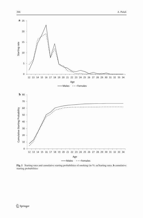
Figure 1 highlights unconditional dynamics of starting age of smoking in the sample.Panel (a) displays the empirical hazard rates of tobacco uptake for both males andfemales. The figure shows that starting rates make a peak at the age of 16 and thenanother—smaller peak at the age of 18 for both males and females. The first peak
6 Note that the percentage of respondents in the first two categories of the education attainment variable issomehow low. However, this does not create identification problems. Lumping the first two categories didnot change any of the empirical results and conclusions.
123
Early Smoking, Education, and Labor Market Performance 231
indicates that, conditional on not smoking before, individuals have the highest riskof smoking at the age of 16.7 Starting rates virtually become zero after the age of 25for males and 23 for females; indicating that those who do not start smoking untilmid 20s are very unlikely to do so afterwords. In other words, individuals mature outof smoking risk in their mid 20s regardless of gender. This finding is replicated bythe cumulative starting probability figures in panel (b), where the slope of cumulativeprobability becomes almost zero around the age of 23 for females and 25 for males.The vertical axis displays the probabilities where the slope of cumulative probabilitybecomes almost zero; indicating that more than 60% of females and 65% of malesstart using tobacco at some point in time.
“Appendix 2” presents the details and the descriptive statistics of the control vari-ables and the variables of interest. The second row on the right panel shows that around25% of the individuals, male or female, start using tobacco before the age of 15. Thefirst sub-panel on the right presents the statistics of education variables and shows that,for both males and females, approximately 10% of the respondents have a universitydegree. Most individuals obtain an applied or a higher vocational degree. Around 4%of the respondents report that their education level is below the compulsory educationin the Netherlands (a VMBO degree).8 The last two sub-panels present the statisticsof labor market performance variables. A quick comparison of the figures in the tablereveals that there is an upward movement. The percentage of individuals having alower ranked job is smaller in the current job variable whereas that having a higherranked job is larger. Since the individuals can move upward in the job rankings afteryears of experience, this observation is reasonable.
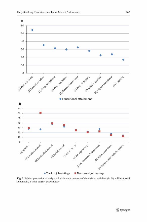
Figure 2 displays the percentage of early smokers in each category of the orderedvariables. For males, there is a clear pattern showing that lower ranked categories aremostly filled with early smokers. For females, as can be seen in Fig. 3, there seems tobe no obvious pattern in educational attainment and labor market performance. Thisunconditional and purely descriptive evidence suggests that there is a negative asso-ciation between early smoking and educational attainment as well as early smokingand labor market performance for males. Whether this association is causal or not isan empirical question.
3 Empirical Model
3.1 Dynamics of Smoking
Two main components of the smoking dynamics are analyzed: starting rates and quitrates. In the starting rates analysis, I assume that individuals become vulnerable to therisk of smoking from age 13 onwards, as only a handful of respondents report a smallerstarting age. Specification of the starting rate at time t (t = 0 at age 12), conditional
7 As of 2013 the sale of tobacco to people under 18 is illegal in the Netherlands. However, the legal agebefore 2013 was 16, which explains the peak at the age of 16.8 Note that for these cases it is not possible to identify if the early smoking takes place before the educationis over. However, assuming that early smoking effect exists for only those with (education > 2) does notchange the results as the percentage of those with (education < 3) is very small.
123
232 A. Palali
on observed characteristics x and unobserved characteristics u, is
θs(t | x, u) = λs(t) exp(x ′βs + u
)(1)
where βs represents the effects of independent variables; λs(t), individual duration(age) dependence. u denotes Heckman and Singer type discrete unobserved hetero-geneity (Heckman and Singer 1984), which is unmeasurable set of differences inindividuals’ susceptibility to smoking. Duration (age) dependence has a form of flex-ible step function; λs(t) = exp(�kλk Ik(t)), where k (= 1,…,9) is a subscript for agecategories. Ik(t) presents time-varying dummy variables that are one in subsequentcategories, 8 of which are for individual ages (age 13, . . . , 20) and the last interval isfor ages above 20. Given that the model has a constant term in x ′βc, the first parameterin duration dependence, λ1, is normalized to 0.
Similar to starting rates of smoking, quit rates are also assessed using a durationmodel. The LISS panel includes questions on the last month use of tobacco. Thespecification below assumes that if an individual reports no use of tobacco in the last30 days, that individual quit smoking in the time period starting from the first use oftobacco until 30 days prior to the survey. Specification of the quit rate at time τ (τ =0 at the age of initiation), conditional on observed characteristics x1 and unobservedcharacteristics v, is
θq(τ | x1, v) = exp(x ′1βq + v
)(2)
Note that this analysis does not contain any duration dependence, because observingthe exact time of quitting in terms of respondents’ ages is not possible. However,interval censored nature of the data allows for the quit duration analysis (i.e., totalduration of use) thanks to the information on the year in which the first use of tobaccotakes place. This information gives an interval for quit duration; in other words, eventhough total duration of smoking is not observed, minimum and maximum values ofthis duration are known. Explicitly, duration of smoking, denoted by τ , will lie in theinterval [0,τq ] where τq is the difference between age at the time of survey and theage of the first use.
The joint density of completed durations until initiation of smoking and completeddurations of smoking is specified as9:
g1(t, τ | x, x1) =∫
v
∫
ufs(t | x, u) fq(τ | x1, v)dG(u, v) (3)
where G(u, v) is the discrete joint mixing distribution of unobserved heterogeneitywhich allows for the possibility that conditional on the observed characteristics, start-ing age of smoking and total duration of smoking are correlated through unobservedcharacteristics. The number of support points inG(u, v) is not predetermined and cho-sen using the likelihood ratio tests. For example, G(u, v) can have 3 points of support(u1, v1), (u1, v2), (u2); with v2 = u2 = −∞. The associated probabilities denoted as
9 Details of the econometric specification are given in “Appendix 4”.
123
Early Smoking, Education, and Labor Market Performance 233
Pr(u1, v1) = p1, Pr(u1, v2) = p2 and Pr(u2) = p3 are assumed to follow a logisticdistribution, pi = exp(αi )
�3i=1 exp(αi )
, where α3 is normalized to zero. This indicates that the
model identifies three types of individuals regarding starting and quitting smoking.The first group consists of individuals with a positive starting and positive quit rate.The second group consists of those with a positive starting rate but a zero quit rate.The third group has a zero starting rate, therefore the quit rate does not exist at all.
3.2 Educational Attainment and Labor Market Performance
I use ordered probit models to investigate how early smoking affects educationalattainment and labor market performance. First, I assume that the smoking decision isindependent from all the unobserved factors than can be correlated with educationalattainment, i.e. that the smoking decision is exogenous. Given that such an assumptionis, by and large, not plausible, the following section (Sect. 3.3) will present the modelthat takes account of possible endogeneity.
Educational attainment is measured as an ordinal variable in a scale of 1–9. Toexploit the ordinal character of the dependent variable, I use an ordered probit modelwith discrete unobserved heterogeneity. Such unobserved heterogeneity captures time-invariant person specific unobserved factors that cause systematic differences ineducational attainment. The unobserved latent variable in the ordered probit model is
y∗ed = x ′βed + ρedsmoke15− + εed + eed (4)
where ρed represents the effect of early smoking. εed controls for discrete type ofunobserved heterogeneity, which is different from the error term eed . Furthermore,βed measures the effect of the control variables. The observed ordered categories andthe rest of the specification of the ordered model are given in “Appendix 4”.
Similar to educational attainment, labor market performance is also investigatedthrough an ordered probit model. The unobserved latent variable in the analysis oflabor market performance is
y∗j = x ′β j + φ j education + ρ j smoke15− + ε j + e j (5)
whereρ j represents the effect of early smoking.φ j controls for the effect of educationalattainment on labor market performance. ε j controls for discrete type of unobservedheterogeneity. β j measures the effect of the control variables. The rest of the analysis isanalogous to the analysis of educational attainment; therefore, the details of the modelspecifications are omitted.The analysis of labor market performance is the same forthe initial and the current job rankings.
3.3 Joint (Correlated) Model
Assuming that smoking is exogenous to educational attainment and labor market per-formance might be unrealistic. The exogeneity assumption requires that the earlysmoking decision is orthogonal to any factor that affects educational attainment andlabor market performance. It is, however, likely that there are unobserved personal
123
234 A. Palali
characteristics that affect all three processes. Some individuals, to exemplify, canexhibit myopic behavior in general by opting for immediate pleasure rather than longterm achievement. If such a behavior is formed early in life, then these individualswill be more likely to smoke at an early age and will be less likely to complete higherlevels of education and less likely to invest in human capital. Thus, an estimated neg-ative effect of smoking will reflect a correlation rather than causality. Distinguishingcausality from correlation by relaxing the exogeneity assumption is crucial to explorethe true effects of early smoking.
To distinguish causality from correlation, I adopt a model that controls for corre-lation between unobserved heterogeneity affecting the smoking decision, educationalattainment and labor market performance. To establish a causal effect, all processesare modeled simultaneously such that unobserved factors are allowed to be corre-lated by using discrete mixing distributions. This correlated discrete factor approachis equivalent to a correlated random effects model. The main idea is that unobservedheterogeneity affecting these three processes can be correlated, i.e. they come from ajoint mixing distribution. This is akin to assume that the endogeneity of the smokingdecision stems from unobserved time invariant factors affecting early smoking andeducational attainment, such as innate ability or rate of time preferences.10 Since theearly smoking decision is taken before the age of 15, reverse causality is not an issuehere. Therefore, this assumption fits well in the empirical question that this studyinvestigates. In the absence of reverse causality, this method corrects the endogeneityproblem stemming from possible omitted variables.
The joint density function of the completed duration of smoking initiation, durationof smoking, educational attainment and labor market performance—g3(t, τ, yed =ked , y j = k j | x, x1, x2,ed , x2, j ) is specified as:
where G(u, v, εed , ε j ) is a discrete mixing distribution underlying unobserved het-erogeneity affecting age of onset of smoking, duration of use, educational attainmentand labor market performance.
4 Parameter Estimates
4.1 The Dynamics of Smoking
Table 5 presents the parameter estimates of mixed proportional hazard models forstarting and quit rates, for both males and females. The negative coefficient estimateson religiosity and age-cohort dummies show that individuals who were living withreligious parents during their adolescence and individuals who belong to older birth
10 Indeed, Kang and Ikeda (2014) show that time preferences related to smoking are interpersonal ratherthan being intra-personal. Thus, they are persistent over time.
123
Early Smoking, Education, and Labor Market Performance 235
cohorts have smaller hazard rates. In other words, they have a lower probability ofinitiating smoking. Moreover, males in couples seem to have higher quit rates com-pared to singles. In addition, those who start smoking at early ages are less likely toquit smoking. The parameter estimates for females display very similar results. Panel(b) in Table 5 presents the estimates for duration (age) dependence parameters. In linewith the patterns observed in Fig. 1, smoking initiation makes a peak at the age of 16and then a smaller peak at the age of 18 for both gender groups.
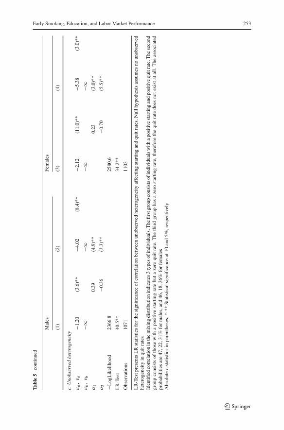
Panel (c) in Table 5 presents the parameter estimates of unobserved heterogeneity.In all columns, I set the second mass points to minus infinity, thereby allowing for thepossibility of zero starting and quit rates. Columns (2) and (3) show that three masspoints are identified in the joint mixing distribution. The finding of 3 points of supportsuggests that there are three types of individuals regarding starting and quitting smok-ing. The first group consists of individuals with a positive starting and positive quittingrate. The second group consists of those with a positive starting rate but a zero quittingrate; the third group, those with a zero starting rate. For the last group, therefore, quit-ting rate does not exist at all. The parameter estimates of probabilities associated tothese mass points show that 47% of the males and 45% of the females have a positivestarting rate and a positive quitting rate; 22% of the males and 18% of the femaleshave a positive starting rate but a zero quitting rate. 31% of the males and 37% of thefemales have a zero starting rate. Finally, the log-likelihood test statistics presentedin the same panel shows that correlation between unobserved heterogeneity affectingstarting rates and quit rates is statistically significant.11 Therefore, it is important tojointly model starting and quit rates to identify the unobserved heterogeneity behindthe dynamics of smoking.
4.2 Educational Attainment
Table 6 displays the estimated parameters of individual and correlated ordered probitmodels. Columns (1) and (3) show that early smoking has a negative associationwith educational attainment for both males and females. As clarified before, theseregressions ignore the possible endogeneity of the smoking decision. Accordingly,the parameter estimates are bound to be inconsistent.
Columns (2) and (4) present the results of the joint models that control for the pos-sible correlation between unobserved heterogeneity affecting education and smoking.As can be seen in both columns, the parameter estimate of the early smoking effectdecreases in size. For females early smoking does not have a causal effect on theeducational attainment, and previously reported negative effect is purely due to thecorrelation through unobserved factors. For males, on the other hand, even though thecoefficient estimate decreases in the joint model, it remains significant. Therefore, Icannot rule out the possibility that early smoking has a causal effect on educationalattainment for males. Finally, the statistics for likelihood ratio tests that appear in panel
11 However, note that a formal LR test is problematic since one of the parameters (α) is not identifiedunder the null hypothesis. This will be the case in the other LR tests reported in this study where the nullhypothesis characterizes no unobserved heterogeneity case.
123
236 A. Palali
(c) show that correlation between unobserved heterogeneity affecting education andsmoking dynamics is statistically significant.12
Admittedly, the finding that early smoking has a causal effect on education mightseem surprising. One can argue that a few years of smoking would not possibly causesignificant health problems that can impair the youth and prevent him or her fromcompleting education. Such an argument has, of course, merit for the current analysisas well because even those who start using tobacco at an early age will not consumeit for long years before they finish their education. Undeniably, certain adverse healtheffects can naturally be observed if individuals use tobacco early. Some of such affectsare briefly discussed before. However, for the sake of the argument, I assume thatthese effects are not observed. If negative health effects are not driving the significantresults presented in Table 6, and if none the other mechanisms discussed before isstrong enough for an early smoking effect, then what can explain the results?
An alternative mechanism is the possibility of exogenous time-varying shocks thatcan simultaneously affect educational attainment and the smoking decision. For exam-ple, loss of a friend or a family member or parental divorce can cause frustration anddepression; resulting in both lower education and involvement in risky health behav-iors including smoking. Panels (a) and (b) of Table 7 attempt to control for some ofsuch possibilities. Panel (a) introduces a dummy variable for early loss of parent(s);panel (b), a dummy variable for early parental divorce. In both cases, “early” meansthat the mentioned frustrating and depressive event takes place before the age of 15.Under both specifications the smoking effect remains unchanged; therefore, I concludethat the early smoking effect is robust to exogenous childhood shocks.
One can alternatively argue that the proposed joint model is unable to captureunobserved factors affecting the smoking decision and educational attainment. Toinvestigate such a possibility I perform several robustness analyses by introducingcontrol variables that are expected to be highly correlated with the unobserved factorsthat can affect both processes. One of such unobserved factors could be systematic dif-ferences between the rate of time preferences between individuals. If such preferencesare formed early in life, then they can explain the negative coefficient estimates ofearly smoking. Individuals with high rates of time preference will place a higher valueon present than on future. Consequently, they will be more likely to enjoy risky healthbehaviors and less likely to invest in human capital (Levine et al. 1997). In panel (c) ofTable 7, I control for certain preference patterns to check the robustness of the smok-ing effect. If the early smoking effect changes after adding the preference variables,then it means the joint model fails to capture unobserved systematic differences. Thepreference patterns for which the specification controls are risk aversion, prudenceand temperance. “Appendix 3” gives more information on the measurement and theuse of these preference variables. For both males and females, parameter estimates inthe table show that the results do not change; therefore, such preferences are alreadycaptured by the joint model and not driving the main results.
12 Note that in this education estimation late starters, those who start smoking after the age of 14, are inthe reference group. Therefore the early smoking effect can be actually a lower bound for the actual effectof smoking on education. Lower panel of Table 6 presents the results after I add another dummy variablefor those who start smoking after the age of 14. The early smoking effect does not change.
123
Early Smoking, Education, and Labor Market Performance 237
Another unobserved factor can be the selection into peer groups. For any risky healthbehavior, peers can have an effect on the individual. If for example, certain studentsselect into certain peer groups, their education and smoking behavior can be affectedsimultaneously. It should be noted that current econometric model is exactly designedfor such unobserved factors. If individuals select into peer groups based on someunobserved factors before smoking initiates, then this will be captured by the model.If selection happens after smoking initiates, based on the smoking behavior, then thisis a consequence of smoking rather being a problem. Even though the econometricmodel is designed to capture such issues, I performed several sensitivity analysis usingproxies for peer effects. Panel (d) of Table 7 introduces control variables for parentaleducation. The smoking effect is robust to the inclusion of these variables. Finally, thelast panel of Table 7 displays the results of an estimation where I include a dummyvariable for the early use of alcohol (before age of 15). There is no data on the peer useof tobacco during childhood. Therefore, the idea here is that the peer effects that canlead an individual to use tobacco can also lead the same individual to involve in otherrisky health behaviors such as early alcohol use. In other words early alcohol use canbe used as an imperfect proxy for the general peer effects. The results show that theearly smoking effect is unchanged.13 All in all, the results of these sensitivity checksshow that the joint model successfully controls for correlated unobserved factors thatcan jointly affect the smoking decision and educational attainment.
Finally, the remaining mechanism possibly explaining the negative smoking effectis that early smoking has indeed a causal effect on education via the various channelsmentioned before.14 Unfortunately the data at hand does not allow for exploration ofthese mechanisms for there is no information on physical or mental health of individ-uals at young ages, or on attendance patterns at schools. If there is indeed a causaleffect, then those who start smoking at an early age unintentionally enter a differentlife-labor path. Subsequently, such an early path diversion between smokers and non-
13 In unreported estimations I also included a dummy for the early cannabis use. The coefficient estimatefor the smoking effect is −0.26 and −0.09 for males and females, respectively. However, there are only ahandful of individuals who start using cannabis before the age of 13. The results are also robust to inclusionof peer use of tobacco at the survey time. If selection into peer groups persists, then controlling for currentpeer use of tobacco can be used as a proxy for peer use in childhood.14 One special aspect of the Dutch education system is that the students are assigned to different types ofsecondary school after the age of 12 based on their academic success. That means it is possible that certaintypes of kids get together in different types of schools, which can affect the smoking behavior. In such a caseit is hard to assume no-reverse-causality. Even though I try to control for possible peer effects in a reportedestimation, I investigate the effects of this early assignment into schools. I performed the baseline jointanalysis with a new early smoking dummy which takes a value of 1 if the respondent starts smoking beforethe age of 13 (the age at which they are in the assigned secondary school). This new analysis cannot sufferfrom any possible reverse causality because for these starters the provided education is exactly the same.The estimated coefficients for this new early smoking dummy are −0.23 for males, and 0.01 for females.Even though there are only a few individuals starting smoking before the age of 13, reverse causality doesnot seem to be an issue. The new coefficients are very similar to the baseline results, albeit impreciselyestimated.
In an alternativemethod, I checked the robustness of the early smoking effect by introducing educationalattainment dummies into the starting rates analysis. Even though this estimation is not perfect due to theunavailability of information on the early education tracks of the respondents, it serves well as a sensitivityanalysis. The results showed that the negative early smoking effect for males is robust. Full estimationresults are available upon request.
123
238 A. Palali
smokers can result in serious disadvantages for the former through the accumulationof the effects. The following section will partly shed light on 2 of these disadvantagesby presenting the analysis of the first and the current job rankings.
4.3 Labor Market Performance
4.3.1 The First Job Rankings
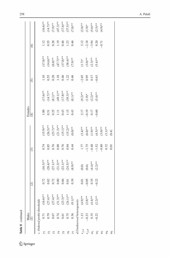
Table 8 presents the coefficient estimates of the joint models on the first job rankingsfor males and females. The first column suggests that the early smoking decision hasa negative effect on the type of the first job that a male has. Nonetheless, this effectalters once the specification includes educational attainment variables. Consideringthe discussion about the effects of early smoking on education in the previous section,one can indeed expect a change in the coefficient estimate. However, the change isso manifest that as presented in the second column of the table, keeping the level ofeducation constant, early smoking does not affect the first job. Considering the afore-mentioned mechanisms through which smoking can affect labor market performance,this empirical finding is reasonable. For the first jobs, no employer discrimination isexpected as the smoking status of the first time job applicants will not be observ-able. Moreover, the serious health consequences that can affect the productivity areprobably not observed since they take place after long years of use. The remainingmechanism is the educational attainment, which is what the results also indicate.
Additionally, column (3) controls for possible endogeneity of the educational attain-ment in the first job rankings estimation. The coefficient estimate of early smoking isunchanged; showing that it is robust to the extension of the functional form definingunobserved heterogeneity. The last three columns present the same results for females.For both gender groups, statistics of likelihood ratio tests that appear in panel (d) revealthat the correlation between unobserved heterogeneity affecting smoking dynamics,education and the first job rankings is significant. Therefore, estimations that fail incontrolling for this correlation would suffer inconsistency.
Table 9 presents the results of various sensitivity analysis on the joint model formales and females, respectively. The first sensitivity analysis controls for the pref-erence patterns to take account of different rate of time preferences, prudence andpatience. Although the sample size decreases substantially, a quick comparison withthe columns (3) and (6) of Table 8 reveals that the results remain similar. The secondsensitivity analysis controls for the search efforts before an individuals finds his or herfirst job. Similar to the previous sensitivity analysis, the purpose is to take account ofdifferent preferences. This sensitivity analysis also takes account of possible exoge-nous shocks that can impair abilities to put search effort. The results show that thecoefficient estimate of early smoking is robust to this specification for both gendergroups. The final sensitivity check controls for possible calendar effects by introducingthe year in which an individuals starts his or her first job. The results are also robustto this final specification for both gender groups.
All in all, the results indicate that early smoking has an adverse effect on the first jobrankings, but only through education. Therefore, if the academic problems stemming
123
Early Smoking, Education, and Labor Market Performance 239
from early smoking can be prevented, early smokers will be less likely to start theircareer in the labor market from a disadvantaged point. Admittedly, the first job is onlya part of the life-time labor market performance, and the next section will explore thepossible long-term effects of early smoking by investigating the effects on the currentjobs of individuals.
4.3.2 The Current Job Rankings
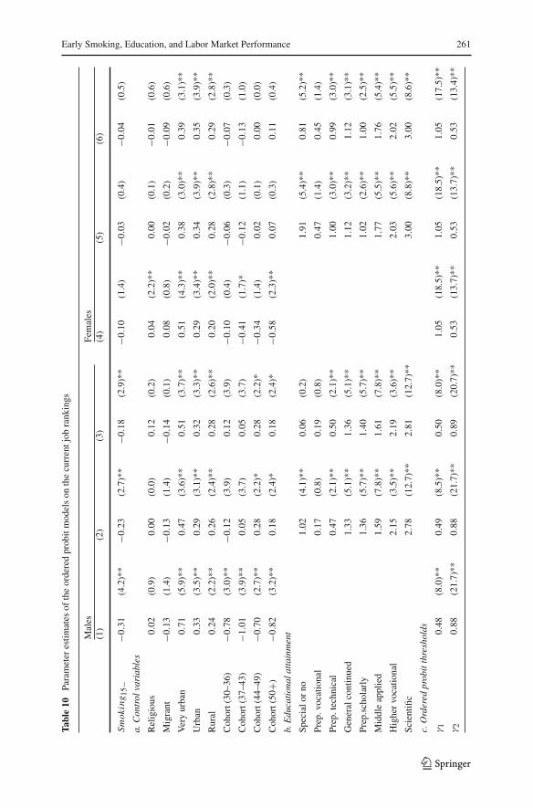
Table 10 presents the parameter estimates of the current job ranking regressions.15
Column (1) in Table 10 present the results when educational attainment is notcontrolled for. Column (2) adds the educational attainment dummies into the analysis.Comparing the coefficient estimates of early smoking in columns (1) and (2) showsthat, similar to the first job rankings, early smoking has an effect on the current jobrankings through education for males.
Column (2) shows the estimates of individualmodel formales, where early smokingis assumed to be exogenous. There is a negative and significant association betweenearly smoking and the current job rankings. Column (3) presents the results of thecorrelated model, where the correlation between unobserved heterogeneity is takeninto account. The coefficient estimate of early smoking decreases from column (2) tocolumn (3). However, it remains significant.16 Columns (5) and (6) present the resultsfor females. Neither in the individual model nor in the joint model there is evidencefor a negative effect. Likelihood ratio tests show that the joint model is preferred overindividual models, which ignore the correlation between unobserved heterogeneity.
Contrasting the results in the previous section with the ones here shows that there isa difference between the first job rankings and the current job rankings in terms of theearly smoking effect. Even though there is no evidence for the early smoking effect onthe first job rankings (conditional on education), the results in Table 10 show that thereis an effect on the current job rankings. Statistically, there can be two main reasonsfor such a phenomenon. The first is that those who start smoking at an early age aremore likely to move downward in the labor market performance rankings, comparedto those who do not start smoking early. The second is that early smokers are less likelyto move upward. Since there are only a handful of observations where the first job ishigher ranked than the current job, the second explanation sounds more plausible.
To check if early smokers are indeed less likely to more upward, I perform a similarordered probit estimation, where the dependent variable is the difference between the
15 Note that there might be a selection bias in the ranked information on jobs since the ranking exists forindividuals who select into employment. In order to check if this is a serious problem in the data at hand,I re-estimated the simple ordered probit model by re-categorizing the job rankings. In the new rankings Iset the first category for those who do not have a paid job. The remaining categories are kept the same. Theresults and interpretation of this estimation remain the same.16 One caveat in the current job rankings estimations is that cohort effects can be important. The reason isthat since the current job information is collected for everyone in the sample in the same year, young cohortsare less likely to have a current job which is different than their first job. Ideally age categories control forsuch an effect because they serve as cohort dummies. Moreover, I also included a variable to control forthe years elapsed from the moment respondents started working in their first jobs until the survey time. Theresults did not change, because as expected this new variable is highly correlated with the cohort dummies.
123
240 A. Palali
current job rankings and the first job rankings. This variable takes a value of 1 if thereis no change or the difference is negative; 2 if the difference is 1; 3 if the difference is2; and 4 if the difference is more than 2. Table 4 displays the sample statistics of thesejob transitions. The parameter estimates are reported in Table 11. Since the chancesof moving upward in the rankings can depend on the initial position, I also controlfor the first job type. Coefficient estimate of early smoking shows that males whostart using tobacco at an early age are less likely to move upward in the job rankings.This inertia explains why there is no effect on the first job, but there is on the currentjob. This finding is in line with the expected long term adverse effects of smoking(especially on physical health). Apparently, the accumulation of effects distorts labormarket performance and harms individuals’ ability tomove upward in the job rankings.
Finally, Table 12 succinctly connects the labor market effects of early smokingto the wider literature on the wage effects of tobacco consumption. The dependentvariable, in this estimation, is the log hourly wages of the individuals calculatedas Monthly wages
hours worked per week∗4.29 . For hourly wage estimations, I use information from
individuals who report at least 20h of work per week or at most 60.17 Unlike the fore-going sections, the dependent variable is not an ordered one in this case. Therefore,“Appendix 4” briefly presents the econometric model that produces the parameter esti-mates in the table. The main idea behind the estimation is the same; the joint modelallows for correlation between unobserved heterogeneity affecting hourly wages,smoking dynamics, education and job rankings.18
In order to analyze the effect of early smoking, I initially include the early smokingdummy and the available control variables in the wage equation. The results show thatearly smoking negatively affect the wages of males. There seems to be no negativeeffect for females. In order to see the occupation-specific effects of early smoking,I include interactions between the early smoking variable and the job type dummiesinto the wage equation. Lower panel of Table 12 report the results. For almost all ofthe job types of males early smoking negatively affects wages. The effect seems to bethe highest for lower ranked jobs. For females, on the other hand, there is no evidencefor a smoking effect.
Although not reported, I performed several other sensitivity analysis on the currentjob rankings, wages and the probability of switching to a better job. First, I re-estimatedthe effect of early smoking on current labor market performance by using informationabout the current status of smoking. It seems that negative effect on the wages andthe current job is higher for those who start smoking early and continue smoking untilthe time of the survey. However, the coefficient estimate of interaction between earlysmoking and current smoking is imprecisely estimated. The possible reason is that thevast majority of those who start using tobacco before the age of 15 consists of still-
17 These are natural cutoff points in the data. Only a handful of male respondents report working less than20h and more than 60h. One respondent reports 124h of working per week.18 Similar to the ordered probit model on the current job rankings, there might be a selection bias in thewage estimation because wages exists only for those who select into employment. I controlled for the samebias by estimating a simple Heckman’s sample selection model. For both males and females, Mills ratiois found to be insignificant. In short, selection bias due to sample selection is not an issue in the wageestimations.
123
Early Smoking, Education, and Labor Market Performance 241
smokers. Second, I controlled for risk attitudes in the analysis of current labor marketperformance. The reason is that preferences and risk attitudes can affect incentives toinvest further in human capital, e.g. through on the job trainings. The results in Tables11 and 12 are found to be robust to the inclusion of the risk attitude and preferencevariables. Furthermore, using ordered logit models instead of probit ones did not alsochange the results, only rescaled the coefficient estimates.
4.4 Magnitude of the Effects
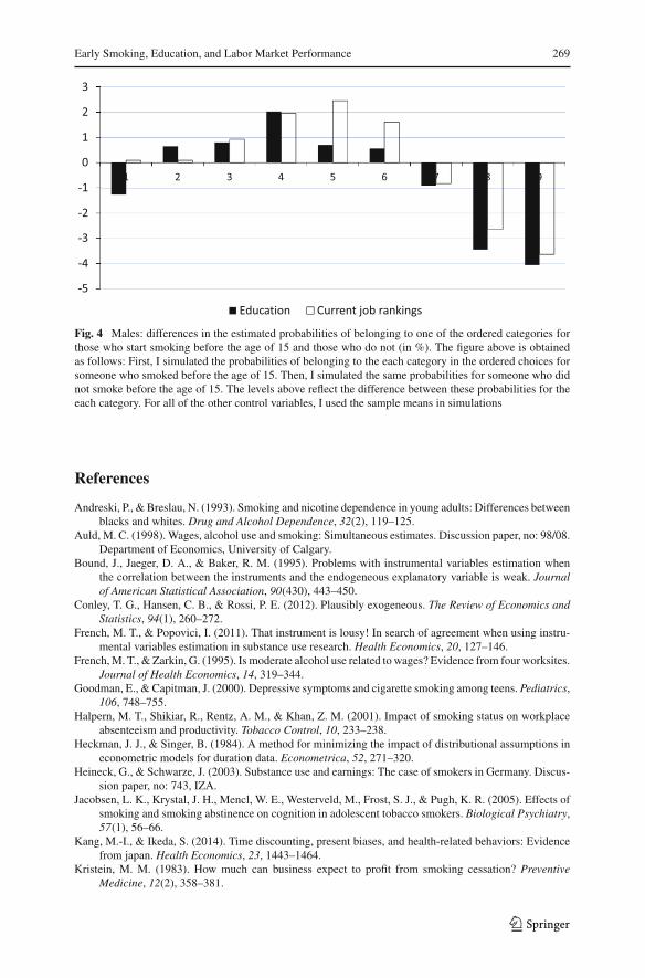
Figure 4 briefly displays the magnitude of the early smoking effect on educationalattainment and the current job rankings for only males. The numbers in the figureare obtained as follows. First, I simulated the probabilities of belonging to the eachcategory in the ordered choices for those who smoked before the age of 15 usingthe estimates presented in column 2 of Table 6 and column 2 of Table 10. Then, thesame probabilities are simulated for those who did not smoke before the age of 15. Thenumbers in thefigure reflect the differences between these probabilities for the each cat-egory. For all of the other control variables, sample means are used in the simulations.
The results show that early smoking decreases the probability of finishing a highlevel of education. The effect is the largest on the probability of finishing a scien-tific degree. The probability of completing scientific education is 4%-point lower forsomeone who smoked before the age of 15. Similarly, early smoking decreases theprobability of having an academic job by almost 4%-point in the long run.
5 Conclusion
There is a small literature studying the causal effects of smoking on labor marketperformance. The majority of the studies within this literature focuses on earningsor hourly wages. The literature on the relationship between smoking and educationalattainment is even smaller. A handful of studies explore the association between smok-ing behavior and education without establishing causal effects.
This study focuses on the effects of early initiation of smoking on educationalattainment and labor market performance. It uses not only hourly wage informationbut also ranking of jobs to measure labor market performance as this information isavailable for both the first jobs and the current jobs. Since educational attainmentand job ranking variables have ordinal character, ordered probit models are used inestimations. The results indicate that there is a strong negative association betweensmoking and education as well as smoking and labor market performance for boththe first job and the current job rankings. However, it is possible that smoking andeducation, and smoking and labor market performance are jointly determined by a setof unobserved factors. To tackle this endogeneity problem, the current study uses acorrelated discrete factor approach, which is equivalent to a correlated random effectsmodel in which the main idea is that unobserved personal characteristics affectingsmoking, education and labor market performance can be correlated. In the absenceof reverse causality, this method yields causal effects as it controls for the endogeneityproblem stemming from omitted variables.
123
242 A. Palali
The results show that early smoking has a negative effect on educational attainmentfor males only. This negative effect is robust to several sensitivity checks such ascontrolling for risk preferences and depressive childhood events. Apparently, smokingdoes not only have long term negative consequences, but also can start affecting one’slife earlier on. Once education is controlled for, there is no evidence for the earlysmoking effect on the first jobs. The only effect seems to be through education. Thiseffect suggests that early smokers start their labor market career from a disadvantagedpoint, and this disadvantage is due to that early smokers perform worse in schools. Nocausal effect is found for females.
Unlike the first job rankings, educational attainment is not the only channel throughwhich early smoking affects the current job rankings of males. The results show thatthere is still an effect on the current job conditional on educational attainment; whichis a finding in line with the existing literature on the wage effects of smoking. Proposedmechanisms for the wage effects of smoking are mainly discrimination, serious healthconsequences and smoking breaks at workplaces. All these mechanisms might workafter years in the labor market. All in all, it seems that the adverse effects of earlysmoking accumulates over time and early smokers who start their career with lowranked jobs become stuck in those jobs or become less likely to make a career. Finally,an analysis of the log-hourly-wages shows that reported wage effects of early smokingmay be due to the possible effects on the type of jobs.
The reported effects of early smoking on educational attainment of males suggestthat policies against smoking, targeting especially youth, can be indeed effective. Itis not only the case that early smoking affects solely education, but it also affectsother important life outcomes through education. Therefore fight against the adverseeffects of smoking needs to begin very early in schools for once the smoking effect oneducational attainment materializes, there might be several long term consequences.If the negative effect of early smoking on education can be prevented, the indirectadverse effects can also be prevented. The easiest way to do so is, of course, to preventyoung individuals from initiation into smoking. This requires a much more detailedanalysis of the determinants of tobacco uptake. Only then it is possible to identify themore vulnerable individuals and fight against the negative aspects of tobacco uptake.Furthermore, the difference between males and females in terms of the early smokingeffect indicates that there is need for further analysis of the mechanisms throughwhich smoking affects education and labor market performance. Apparently, some ofthe proposed mechanisms work only for males.
Finally, the existence of early smoking effect on the current job conditional oneducational attainment suggests that early smoking affects labor market performancethrough other channels in the long run. Apparently, the problems related to earlyinitiation of smoking accumulate, and it is not only the education that matters in thelong run. This further calls for preventive measures.
Compliance with Ethical Standards
Conflict of interest The authors declare that they have no conflict of interest.
Open Access This article is distributed under the terms of the Creative Commons Attribution 4.0 Interna-tional License (http://creativecommons.org/licenses/by/4.0/), which permits unrestricted use, distribution,
Early Smoking, Education, and Labor Market Performance 243
and reproduction in any medium, provided you give appropriate credit to the original author(s) and thesource, provide a link to the Creative Commons license, and indicate if changes were made.
Appendix 1: Ordered Variables
Tables 1 and 2 below show the ordered categories of the education and the job rankingvariables. In the Netherlands, currently, the compulsory education ends at the age of16; corresponding to a VMBO degree. Any of the other degrees are based on voluntary
9 Higher academic or independent job (e.g.,physician, scholar)
25.4 20.7
123
244 A. Palali
education. Due to the changes in the education system, name of the degrees obtainedby the older part of the sample may be different. For those cases, I used the currentcategories that correspond to the old ones, according to CBS (Statistics Netherlands).
The information on jobs come jointly fromWorking and Schooling andWage Indi-cator data sets. The first job and the current job have the same categories, disregardingside jobs and holiday jobs. The columns on the right display the average hourly wages(in Euros) for each category. There are other variables which might possibly be used inthe ordering of the jobs. However, for none of these variables such as satisfaction withjob, satisfaction with wages or working hours there is enough variation between jobcategories. It seems that almost all of the respondents have similar levels of satisfactionwith their jobs, wages or working hours regardless of the job that they have.
Appendix 2: Descriptive Statistics
Definition of the variables used throughout this study and their summary statistics aregiven below (Tables 3 and 4):
• Smoke: Dummy variable with a value of 1 if individual ever used tobacco; 0otherwise.
• Smoking15− : Dummy variable with a value of 1 if individual used tobacco beforeage of 15; 0 otherwise.
• Background variables.– Religious: Amount of the times that the parents of the respondent visited thechurch in a week when the respondent was 15 years old.
– Migrant:Dummyvariablewith a value of 1 if individual ismigrant; 0 otherwise.
• Cohort effects
– Cohort (30−) (Reference): Dummy variable; 1 if aged below 30; 0 otherwise.– Cohort (30–36): Dummy variable; 1 if aged between 30 and 36; 0 otherwise.– Cohort (37–43): Dummy variable; 1 if aged between 37 and 43; 0 otherwise.– Cohort (44–49): Dummy variable; 1 if aged between 44 and 49; 0 otherwise.– Cohort (50+):Dummy variable; 1 if aged above 50; 0 otherwise.
• Urbanization level
– Very urban: Dummy variable with a value of 1 if the municipality of residenceis very urban (population density per km2 is above 2500); 0 otherwise.
– Urban: Dummy variable with a value of 1 if the municipality of residence isurban (population density per km2 is between 1000 and 2500); 0 otherwise.
– Rural: Dummy variable with a value of 1 if the municipality of residence isrural (population density per km2 is between 500 and 1000); 0 otherwise.
– Very rural (Reference): Dummy variable with a value of 1 if themunicipality ofresidence is very rural (population density per km2 is below 500); 0 otherwise.
• Domestic situation
123
Early Smoking, Education, and Labor Market Performance 245
Table 3 Descriptive statistics of the variables
Males Females
Mean SD Mean SD
Variables of interest
Smoke 0.69 0.46 0.64 0.48
Smoke<15 0.26 0.45 0.24 0.43
Educational attainment
Primary or no 0.02 0.15 0.02 0.12
Special or other 0.02 0.15 0.03 0.16
Prep. vocational 0.11 0.32 0.1 0.29
Prep. technical 0.11 0.32 0.13 0.34
General continued 0.05 0.22 0.06 0.24
Prep. scholarly 0.05 0.21 0.03 0.17
Middle applied 0.26 0.44 0.29 0.45
Higher vocational 0.24 0.43 0.26 0.44
Scientific 0.13 0.34 0.09 0.28
The first job rankings
Agrarian 0.05 0.21 0.01 0.1
Unskilled manual 0.07 0.26 0.08 0.27
Semi-skilled manual 0.16 0.37 0.05 0.21
Skilled manual 0.16 0.37 0.01 0.12
Other clerical 0.2 0.4 0.42 0.49
Int. supervisory 0.12 0.33 0.07 0.25
Int. academic/independent 0.13 0.34 0.31 0.46
Higher supervisory 0.02 0.14 0.02 0.12
Higher academic/independent 0.08 0.27 0.03 0.18
The current job rankings
Agrarian 0.03 0.17 0.01 0.1
Unskilled manual 0.02 0.13 0.08 0.26
Semi-skilled manual 0.1 0.3 0.04 0.2
Skilled manual 0.13 0.34 0.02 0.12
Other clerical 0.16 0.37 0.32 0.47
Int. supervisory 0.18 0.38 0.1 0.3
Int. academic/independent 0.17 0.38 0.34 0.47
Higher supervisory 0.12 0.32 0.05 0.22
Higher academic/independent 0.1 0.3 0.05 0.22
Control variables
Religious 2.14 1.87 2.15 1.89
Migrant 0.14 0.34 0.11 0.32
Urbanization dummies
Very urban 0.11 0.32 0.12 0.33
Urban 0.51 0.44 0.49 0.43
123
246 A. Palali
Table 3 continued
Males Females
Mean SD Mean SD
Rural 0.22 0.41 0.21 0.41
Very rural 0.16 0.37 0.18 0.38
Domestic situation
Single wo. children 0.14 0.35 0.13 0.34
Married wo. children 0.3 0.46 0.29 0.46
Married w. children 0.52 0.5 0.5 0.5
Single w. children 0.03 0.16 0.07 0.25
Cohort dummies
Cohort (30−) 0.07 0.12 0.07 0.15
Cohort (30–36) 0.18 0.38 0.21 0.41
Cohort (37–43) 0.29 0.46 0.28 0.46
Cohort (44–49) 0.31 0.47 0.32 0.47
Cohort (50+) 0.15 0.4 0.11 0.35
Risk attitudes
Risk averse 0.45 0.5 0.6 0.49
Prudence 0.57 0.49 0.57 0.5
Temperance 0.43 0.5 0.49 0.5
Parents’ education
Mother edc 4.36 2.88 4.27 2.53
Father edc 5.27 3.1 5.35 3.19
Childhood events
Parents death 0.04 0.18 0.03 0.18
Parent divorced 0.04 0.19 0.05 0.21
Search efforts (first job)
No search 0.46 0.5 0.42 0.49
Short search 0.33 0.47 0.39 0.49
Moderate search 0.11 0.31 0.09 0.29
Intensive search 0.1 0.31 0.11 0.31
Moderate search 0.11 0.31 0.09 0.29
Intensive search 0.1 0.31 0.11 0.31
– Single wo. children (Reference): Dummy variable; 1 if individual is singlewithout children; 0 otherwise.
– Married wo. children: Dummy variable with; 1 if individual is married withoutchildren; 0 otherwise.
– Married w. children: Dummy variable with; 1 if individual is married withchildren; 0 otherwise.
– Singlew. children:Dummyvariablewith; 1 if individual is singlewith children;0 otherwise.
123
Early Smoking, Education, and Labor Market Performance 247
Table 4 Job transitions (from the initial job rankings to the current job rankings)
Males Females
Mean SD Mean SD
The current job < the first job 0.03 0.18 0.09 0.29
The current job = the first job 0.54 0.50 0.66 0.47
The current job > the first job 0.43 0.50 0.25 0.43
The current job = the first job +1 0.13 0.34 0.08 0.28
The current job = the first job +2 0.14 0.34 0.09 0.29
The current job > the first job +2 0.16 0.37 0.08 0.26
Table 4 shows the percentage of individuals in each category based on the difference between the first jobrankings and the current job rankings
• Risk attitudes
– Risk Aversion: Dummy variable; 1 if the individual displays risk aversion; 0otherwise.
– Prudence: Dummy variable; 1 if the individual displays prudence; 0 otherwise.– Temperance: Dummy variable; 1 if the individual displays temperance; 0 oth-erwise.
• Parental characteristics
– Mother’s education: Highest degree themother of the individual obtained; 1–9.– Father’s education: Highest degree the father of the individual obtained; 1–9.– Parental loss: Dummy variable; 1 if the individual lost at least one of his or herparents before the age of 15.
– Parental divorce: Dummy variable; 1 the parents of the individuals divorcedbefore the age of 15.
• Search efforts before the first job
– No search: Dummy variable; 1 if the individual reports no search effort for thefirst job.
– Short search: Dummy variable; 1 if individual spent less than 1 month to findhis or her first job.
– Moderate search: Dummy variable; 1 if individual spent 1-3 months to find hisor her first job.
– Intensive search (Reference): Dummy variable; 1 if individual spent more than3 months to find his or her first job.
Appendix 3: Additional Data Sets from the LISS Panel
In addition to the three main single wave studies of the LISS panel—Alcohol andDrugs, Working and Schooling, and Wage Indicator—the following two data sets areused in some sensitivity analysis.
123
248 A. Palali
Life History Questionnaire
Life history questionnaire is a single wave study consisting of several parts that con-cern family histories of the respondents. In each part of the survey the respondentsanswer different questions regarding their family situation during childhood. The ques-tionnaire was made available in 2012, and in total 5231 individuals completed thequestionnaire.
Measuring Higher Order Risk Attitudes of the General Population
This single wave questionnaire concerns the measurement of the degree of risk aver-sion, prudence and temperance of respondents by recording answers given to severalchoices between lotteries. The respondents were presented lottery choices after beingassigned to different situations bymeans of randomdice throws. Their choices betweenlotteries are used to measure the risk attitudes.
I use the same strategy in Noussair et al. (2014) to measure the incidence of pru-dence, temperance, and risk aversion. I measure risk aversion with the number of safechoices an individual makes, out of the five decisions involving a sure payoff and arisky lottery. Similarly, I measure prudence with the number of prudent choices, andtemperance with the number of temperate choices that an individual makes. Then, Iassume that an individual is risk averse (prudent, temperate) if the number of choicesis greater than 3. Since the data set used in Noussair et al. (2014) is the same, a moredetailed explanation of the questions and measurement strategy can be found in theirstudy.
Appendix 4: ML of the Starting Rates, Quit Rates, Ordered ProbitModels and the Wage Equation
Starting Rates
The specification of the hazard rate for starting rates (following Eq. 1) yields the fol-lowing functional form for the conditional density function of the completed durationsuntil the uptake of tobacco;
fs(t | x, u) = θs(t | x, u) exp
(−
∫ t
0θs(μ | x, u)dμ
)(7)
Integrating out the unobserved heterogeneity in the conditional density in Eq. 7 givesthe following density function for the duration until tobacco uptake (t) conditional onx , but unconditional on u:
fs(t | x) =∫
ufs(t | x, u)dG(u) (8)
123
Early Smoking, Education, and Labor Market Performance 249
where G(u) is a discrete mixing distribution where the number of support points arechosen based on empirical tests. In case of 2 support points, two types of individualsexist regarding the hazard rate for tobacco uptake: those who are more likely to smokeand those who are less likely to smoke. Each individual has a probability of belongingto one of these types, and the probabilities, being the same for everyone, are denotedas follows: Pr(u = ua) = r and Pr(u = ub + ua) = 1− r . r has a logit specification;r = exp(α)
1+exp(α), where α is the parameter defining the probabilities and to be estimated
by the model. The mixed proportional hazard framework assumes that α does notdepend on any observables, including calendar or age effects.
The log-likelihood that accounts for the discrete nature of the observations on theonset age of smoking is
n∑
i=1
ds,i log [Fs(ti − 1) − Fs(ti )] + (1 − ds,i
)log
[1 − Fs(ts,i )
](9)
where i is an index for individual, n is the number of individuals in the sample andds,i is a dummy variable that is equal to 1 if an individual started using tobacco andequal to 0 otherwise.
Quit Rates
The conditional density function for the completed durations until the last use (fol-lowing Eq. 2) is
where x1 is the set of control variables. v is the unobserved heterogeneity in the quitrates. Integrating out the conditional density function over the interval of maximumand minimum values that the duration can take on, yields the distribution function, Fq
Using the distribution function, Fq , I specify the following log-likelihood for theanalysis of quit rates
m∑
i=1
dq,i log[Fq(τq,i )
] + (1 − dq,i
)log
[1 − Fq(τq,i )
](11)
where m is the number of individuals that ever used tobacco and dq,i is a dummyvariable that has a value of 1 if the individual stopped using tobacco and a value of 0if the individual did not stop using tobacco. Individuals who report using tobacco inthe last 30 days are right censored, i.e. they are assumed to be non-quitters. I performthe quitting analysis using only those who ever use tobacco; otherwise quit rates donot exist. Similar to starting rates I assume that there are 2 unobserved heterogeneitygroups.
123
250 A. Palali
Ordered Probit Models
The observed ordered categories in the data are
yed =
⎧⎪⎪⎪⎪⎪⎪⎪⎨
⎪⎪⎪⎪⎪⎪⎪⎩
1 if y∗ed ≤ μ1
2 if μ1 < y∗ed ≤ μ2
.
.
ked − 1 if μked−2 < y∗ed ≤ μked−1
ked if μked−1 < y∗ed
(12)
where μ’s are to be estimated threshold parameters in the ordered probit model andked is the number of alternatives in the ordered choice; 9. Assuming that the errorterm eed has a standard normal distribution, one can write the following probabilitiesfor the ordered probit model, conditional on observable and unobservable individualheterogeneity19:
Pr(yed = ked |x2,ed , εed ) = �(μked − x ′2,edβed − εed ) − �(μked−1 − x ′
2,edβed − εed ) .
(13)
where �(.) is standard normal cdf. with �(μ0 − x ′2,edβed − εed) = 0 and
�(μ9 − x ′2,edβed − εed) = 1. Since there are heterogeneity specific constants in the
model, I set the first threshold parameter μ1 to zero. The other threshold parametersare modeled in the following way so as to ensure that the probabilities are positive andthresholds are ordered: μ2 = γ 2
ked−2.Analogous to starting and quit rates, integrating out the unobserved heterogene-ity in the conditional probabilities, given in Eq. 13, yields the unconditional ones.Explicitly;
Pr(yed = ked |x2) =∫
εed
Prob(yed = ked |x2, εed)dG(εed) (14)
where k ∈ {1, 2, 3, . . . , 9}, denoting ordered choices. I assume thatG(εed) is a discretemixing distribution. In case that there are 2 support points, conditional on observedcharacteristics, there are 2 types of individuals in the ordered choices on educationalattainment: high education types and low education types. The associated probabilitiesare: Pr(εed = εa,ed) = p and Pr(εed = εb,ed + εa,ed) = 1 − p, where p is modeledusing a logit specification, p = exp(α)
1+exp(α). Finally, the likelihood function of the ordered
probit models is∏
N Prob(yed = ked |x2).
19 For simplicity I write x ′2,edβed = x ′βed + ρed smoke15−
123
Early Smoking, Education, and Labor Market Performance 251
Wage Equation
In order to investigate the wage effects of smoking, I first estimate a simple linearmodel where log hourly wage is a function of early smoking for males and femalesseparately. To take account of unobserved heterogeneity in the wage equation, I use adiscrete factor approach. The wage equation is specified as
wi = β0 + β1x4,i + β2ti + β3dti + ωi + ei (15)
where wi is log hourly wage, xi represents personal characteristics, ti is a dummyindicator of early smoking and dti is the interaction of early smoking dummy with thefirst job ranking dummies. ωi is the unobserved heterogeneity component of the wageequation for hourly wages. ei is the error term. This discrete factor approach makesthe probability density function conditional on unobserved heterogeneity, which canbe integrated out once we assume a functional form. The resulting log likelihood ofthis linear model is
L =N∑
i=1
log
(∫
ω
f (w|x4, ω)dG(ω)
)(16)
where f (.) is the probability density function of the normal distribution and G(ω) isa discrete mixing distribution as in the previous cases.
The joint model—for starting rates, quit rates, education, the current job andwages-is specified as:
where dG(u, v, εed , ε j , ω) is the mixing distribution.
Appendix 5: Estimates
See Tables 5, 6, 7, 8, 9, 10, 11 and 12.
123
252 A. Palali
Table5
Parameter
estim
ates
ofthemixed
prop
ortio
nalh
azardmod
elson
thestartin
gandqu
itratesof
smok
ing
Males
Females
(1)
(2)
(3)
(4)
a.Con
trol
variab
les
Religious
−0.32
(7.3)**
0.01
(0.2)
−0.05
(2.3)**
0.06
(0.8)
Migrant
−0.13
(1.2)
0.12
(0.8)
−0.13
(1.0)
0.40
(1.0)
Veryurban
0.57
(3.8)**
−0.11
(0.5)
0.33
(2.5)
−0.21
(0.5)
Urban
0.27
(2.2)**
0.12
(0.8)
0.21
(1.7)*
−0.30
(0.8)
Rural
0.30
(2.2)**
0.10
(0.6)
0.23
(1.6)
−0.31
(0.7)
Coh
ort(30
–36)
−0.30
(0.8)
−0.15
(0.4)
−0.27
(2.2)**
1.21
(0.5)
Coh
ort(37
–43)
−0.22
(0.7)
−0.85
(2.3)**
−0.56
(3.6)**
−0.58
(0.3)
Coh
ort(44
–49)
−0.37
(1.1)
−1.24
(3.3)**
−0.32
(1.1)
−1.47
(0.9)
Coh
ort(50
+)−0
.10
(0.3)
−1.27
(3.4)**
−0.39
(1.9)*
−1.12
(0.7)
Married
wo.
child
ren
0.57
(3.1)**
0.73
(2.0)**
Married
w.children
0.73
(4.2)**
0.96
(2.6)**
Sing
lew.children
0.25
(0.6)
−0.50
(1.2)
Startin
gage
0.66
(3.8)**
2.23
(4.8)**
b.Age
(duration)
depend
ence
λ20
+0.22
(1.3)
0.11
(0.4)
λ20
0.31
(0.9)
1.30
(4.8)**
λ19
0.74
(2.9)**
1.00
(3.9)**
λ18
1.30
(7.9)**
1.60
(10.4)**
λ17
0.35
(1.8)*
0.66
(3.9)**
λ16
1.22
(9.1)**
1.14
(8.8)**
λ15
0.66
(5.3)**
0.66
(5.1)**
λ14
0.01
(0.0)
0.40
(3.2)**
123
Early Smoking, Education, and Labor Market Performance 253
Table5
continued
Males
Females
(1)
(2)
(3)
(4)
c.Unobservedheterogeneity
ua,
va
−1.20
(3.6)**
−4.02
(8.4)**
−2.12
(11.0)**
−5.38
(3.0)**
ub,
vb
−∞−∞
−∞−∞
α1
0.39
(4.9)**
0.23
(3.0)**
α2
−0.36
(3.3)**
−0.70
(5.5)**
−Log
Likelihoo
d23
66.8
2580
.6
LR-Test
40.5**
34.2**
Observatio
ns10
7111
03
LR-Testp
resentsLRstatisticsforthesignificanceof
correlationbetweenunobserved
heterogeneity
affectingstartin
gandquitrates.Nullh
ypothesisassumes
nounobserved
heterogeneity
inquitrates
Identifi
edcorrelationinthemixingdistributio
nindicates3typesof
individuals.The
firstgroupconsistsof
individualswith
apositiv
estartin
gandpo
sitiv
equ
itrate.T
hesecond
grou
pconsistsof
thosewith
apo
sitiv
estartin
grate
butazero
quitrate.T
hethirdgrou
phasazero
startin
grate,therefore
thequ
itrate
does
notexistat
all.The
associated
prob
abilitie
sare47
,22,
31%
formales,and
46,18,
36%
forfemales
Absolutet-statisticsin
parentheses.*,**
Statisticalsignificanceat10
and5%
,respectively
123
254 A. Palali
Table6
Parameter
estim
ates
oftheorderedprobitmodelson
educationalattainment
Males
Females
(1)
(2)
(3)
(4)
Smok
ing 1
5−−0
.27
(3.5)**
−0.20
(2.6)**
−0.12
(1.7)*
−0.04
(0.5)
a.Con
trol
variab
les
Religious
0.04
(2.0)**
0.04
(2.1)**
0.06
(3.7)**
0.06
(3.5)**
Migrant
0.06
(0.7)
0.06
(0.6)
0.15
(1.6)
0.15
(1.5)
Veryurban
0.43
(3.3)**
0.47
(3.6)**
0.28
(2.2)**
0.28
(2.1)**
Urban
0.09
(0.9)
0.09
(0.9)
−0.04
(0.4)
−0.06
(0.6)
Rural
−0.02
(0.2)
−0.02
(0.1)
−0.12
(1.1)
−0.14
(1.3)
Coh
ort(30
–36)
0.14
(0.3)
0.14
(0.3)
−0.04
(0.1)
−0.01
(0.0)
Coh
ort(37
–43)
−0.28
(0.7)
−0.28
(0.7)
−0.34
(0.8)
− 0.30
(0.7)
Coh
ort(44
–49)
−0.26
(0.6)
−0.25
(0.6)
−0.54
(1.3)
−0.49
(1.2)
Coh
ort(50
+)−0
.34
(1.8)*
−0.33
(1.8)*
−0.87
(2.1)**
−0.83
(2.0)**
b.Ordered
prob
itthresholds
γ1
0.97
(21.5)**
0.98
(20.9)**
0.99
(20.8)**
1.00
(20.7)**
γ2
0.66
(22.7)**
0.66
(22.6)**
0.75
(26.1)**
0.75
(25.8)**
γ3
0.39
(14.5)**
0.40
(14.3)**
0.44
(16.8)**
0.44
(16.5)**
γ4
0.37
(14.1)**
0.37
(13.8)**
0.30
(11.8)**
0.30
(11.8)**
γ5
1.16
(52.6)**
1.17
(51.7)**
1.24
(58.6)**
1.24
(58.0)**
γ6
0.31
(9.8)**
0.31
(9.6)**
0.40
(12.0)**
0.40
(11.9)**
γ7
1.02
(24.3)**
1.02
(24.0)**
0.88
(20.7)**
0.88
(20.3)**
123
Early Smoking, Education, and Labor Market Performance 255
Table6
continued
Males
Females
(1)
(2)
(3)
(4)
c.Unobservedheterogeneity
ε ed,a
2.18
(5.1)**
2.28
(5.2)**
2.56
(6.0)**
2.61
(6.1)**
ε ed,b
−0.39
(4.7)**
−0.33
(3.7)**
α1
0.33
(4.2)**
0.16
(2.1)**
α2
−0.22
(2.3)**
−0.57
(5.3)**
−Log
Likelihoo
d41
99.4
4188
.143
63.3
4356
.6
LR-Test
22.6**
6.7*
*
Observatio
ns10
1710
1711
0311
03
Con
trolling
forthelatesm
okingbeha
vior
Smok
ing 1
5−−0
.36
(3.9)**
−0.22
(2.2)**
−0.15
(1.9)*
−0.04
(0.4)
Smok
ing 1
4+−0
.14
(1.7)*
0.00
(0.0)
−0.18
(2.4)**
−0.10
(1.2)
−Log
Likelihoo
d41
98.0
4187
.543
62.1
4356
.1
Observatio
ns10
1710
1711
0311
03
LR-Testp
resentsLRstatisticsforthesignificanceof
correlationbetweenunobserved
heterogeneity
affectingsm
okingdynamicsandeducation.
Nullh
ypothesisassumes
nounobserved
heterogeneity
ineducation
Forthejointm
odelsonly
thecoefficient
estim
ates
foreducationalattainmentare
presented
Identifi
edcorrelationin
themixingdistributio
nindicates3typesof
individualswith
perfectcorrelatio
nbetweenstartin
gbehavior
andeducationalattainment.The
firstgroup
consistsof
individualswith
apositiv
estartin
g,positiv
equitrateandloweducationalattainment.The
second
groupconsistsof
thosewith
apositiv
estartin
grate,a
zero
quit
rateandloweducationalattainment.The
thirdgrouphasazero
startin
grateandhigh
educationalattainment.The
associated
probabilitiesare45,25,30
%formales,and
43,
20,37%
forfemales
Absolutet-statisticsin
parentheses.*,**
Statisticalsignificanceat10
and5%
,respectively
123
256 A. Palali
Table 7 Parameter estimates ofsensitivity analysis on education
Males Females(1) (2)
a. Early parental divorce
Smoking15− −0.22 (2.5)** −0.01 (0.1)
Parental divorce −0.13 (0.7) −0.14 (1.0)
−LogLikelihood 3089.6 3271.5
Observation 758 825
b. Early parental loss
Smoking15− −0.22 (2.5)** −0.01 (0.1)
Parent loss −0.06 (0.3) −0.09 (1.5)
−LogLikelihood 3089.8 3270.7
Observation 758 825
c. Risk attitudes
Smoking15− −0.19 (2.8)** 0.05 (1.0)
Risk aversion −0.09 (0.9) −0.09 (0.9)
Prudence 0.18 (1.8)* 0.21 (2.0)**
Temperance 0.11 (1.1) 0.11 (1.1)
−LogLikelihood 2426.7 2267.1
Observation 585 579
d. Educational attainment of parents
Smoking15− −0.21 (2.4)** −0.03 (0.3)
Mother’s education 0.01 (0.7) 0.04 (2.6)**
Father’s education 0.03 (1.7)* −0.01 (0.6)
−LogLikelihood 3010.2 3198.8
Observation 737 810
e. Use of alcohol
Smoking15− −0.22 (2.9)** −0.01 (0.9)
Early use of alcohol 0.12 (0.3) 0.34 (0.8)
−LogLikelihood 4187.9 4356.1
Observation 1017 1103
Absolute t-statistics inparentheses. *,** Statisticalsignificance at 10 and 5%,respectively
123
Early Smoking, Education, and Labor Market Performance 257
Table8
Parameter
estim
ates
oftheorderedprob
itmod
elson
thefirstjobrank
ings
Males
Females
(1)
(2)
(3)
(4)
(5)
(6)
Smok
ing 1
5−−0
.16
(2.0)**
−0.07
(0.9)
−0.06
(1.2)
−0.15
(1.8)*
−0.10
(1.4)
−0.07
(1.1)
a.Con
trol
variab
les
Religious
0.01
(0.8)
0.00
(0.0)
0.02
(1.0)
0.05
(3.0)**
0.03
(1.3)
0.05
(3.5)*
Migrant
0.02
(0.2)
0.05
(0.5)
0.08
(0.9)
0.17
(1.7)*
0.09
(0.8)
0.12
(1.8)
Veryurban
0.61
(5.0)**
0.37
(2.8)**
0.55
(3.5)**
0.27
(2.1)**
0.15
(1.7)*
0.17
(1.7)*
Urban
0.32
(3.4)**
0.26
(2.7)**
0.34
(2.9)**
0.08
(0.9)
0.10
(1.1)
0.12
(1.3)
Rural
0.18
(1.7)*
0.16
(1.5)
0.20
(1.4)
0.04
(0.4)
0.09
(0.8)
0.10
(0.9)
Coh
ort(30
–36)
0.49
(2.2)**
0.52
(2.5)**
0.66
(2.1)**
0.18
(0.9)
0.27
(1.4)
0 .25
(1.3)
Coh
ort(37
–43)
0.17
(0.8)
0.40
(2.0)**
0.41
(1.4)
−0.06
(0.3)
0.15
(0.8)
0.14
(0.7)
Coh
ort(44
–49)
0.47
(2.1)**
0.71
(3.5)**
0.67
(2.2)**
0.13
(1.6)*
0.49
(2.6)**
0.48
(2.5)**
Coh
ort(50
+)0.53
(2.3)**
0.83
(3.9)**
0.81
(2.6)**
−0.06
(1.3)
0.44
(2.1)**
0.43
(2.0)**
b.Edu
cation
alattainment
Specialo
rother
0.71
(2.7)**
−0.81
(2.1)**
1.67
(5.8)**
1.84
(5.6)**
Prep.vocational
0.19
(0.8)
0.18
(0.7)
0.35
(1.4)
0.34
(1.4)
Prep.technical
0.54
(2.3)**
0.53
(2.1)**
0.91
(3.7)**
0.91
(3.7)**
Generalcontinued
1.02
(3.7)**
1.06
(3.8)**
1.05
(3.9)**
1.06
(4.0)**
Prep.scholarly
0.92
(3.6)**
0.86
(3.1)**
0.88
(2.4)**
0.89
(2.4)**
Middleapplied
1.25
(6.1)**
0.94
(3.9)**
1.61
(7.2)**
1.63
(7.2)**
Highervocatio
nal
1.85
(6.5)**
0.92
(2.4)**
1.94
(6.4)**
1.95
(6.3)**
Scientific
2.19
(10.0)**
1.26
(4.3)**
2.44
(10.0)**
2.48
(10.1)**
123
258 A. Palali
Table8
continued
Males
Females
(1)
(2)
(3)
(4)
(5)
(6)
c.Ordered
prob
itthresholds
γ1
0.71
(16.6)**
0.72
(16.3)**
0.74
(15.9)**
1.00
(17.6)**
1.10
(17.8)**
1.12
(16.6)**
γ2
0.79
(27.4)**
0.82
(28.4)**
0.85
(26.5)**
0.51
(14.7)**
0.55
(14.6)**
0.55
(14.7)**
γ3
0.67
(27.4)**
0.72
(27.1)**
0.76
(23.7)**
0.25
(8.1)**
0.28
(8.0)**
0.28
(7.9)**
γ4
0.74
(31.3)**
0.80
(31.2)**
0.88
(21.3)**
1.11
(49.1)**
1.18
(47.7)**
1.19
(47.3)**
γ5
0.61
(23.3)**
0.66
(23.1)**
0.76
(15.1)**
0.43
(17.8)**
0.46
(17.8)**
0.46
(17.6)**
γ6
0.75
(24.1)**
0.81
(24.5)**
0.94
(15.2)**
1.15
(39.3)**
1.22
(38.4)**
1.23
(37.5)**
γ7
0.36
(9.1)**
0.39
(8.9)**
0.44
(8.0)**
0.43
(8.1)**
0.46
(7.9)**
0.46
(7.8)**
d.Unobservedheterogeneity
εj,a
1.13
(4.9)**
0.01
(0.0)
1.77
(3.4)**
2.17
(9.2)**
−2.65
(1.7)*
3.12
(2.8)**
εj,b
−0.23
(2.8)**
−0.05
(0.6)
−1.75
(6.0)**
−0.19
(1.9)*
0.95
(3.0)**
−2.18
(1.9)*
α1
0.35
(4.4)**
0.35
(4.4)**
−0.48
(1.9)**
0.17
(2.2)**
0.17
(2.3)**
−3.94
(5.6)**
α2
−0.22
(2.2)**
−0.22
(2.2)**
−1.52
(4.5)**
−0.60
(5.4)**
−0.63
(5.4)**
0.20
(2.5)**
α3
−0.80
(3.0)**
−0.71
(4.9)**
α4
0.32
(3.1)**
α5
0.01
(0.4)
123
Early Smoking, Education, and Labor Market Performance 259
Table8
continued
Males
Females
(1)
(2)
(3)
(4)
(5)
(6)
−Log
Likelihoo
d45
73.4
4442
.060
91.1
4289
.541
72.7
5876
.7
LR-Test-1
26.4**
26.2**
24.1**
30.1**
30.0**
22.2**
LR-Test-2
14.4**
0.6
Observatio
ns10
1710
1710
1711
0311
0311
03
Colum
ns(1)an
d(4)whentheendogeneityof
thesm
okingdecision
isigno
red
Smok
ing 1
5−−0
.19
(2.3)**
−0.20
(2.5)**
LR-Test-1presentsLRstatisticsforthesignificanceof
correlationbetweenunobserved
heterogeneity
affectingsm
okingdynamicsandthefirstjob(for
thelastcolumn,also
education).N
ullh
ypothesisassumes
noun
observed
heterogeneity
inthefirstjob
LR-Test-2presentsLRstatisticsforthesignificanceof
correlationbetweenunobserved
heterogeneity
affectingeducationandthefirstjob
Forthejointm
odelson
lythecoeffic
ient
estim
ates
forjobrank
ings
arepresented
Identifi
edcorrelationin
themixingdistributio
nindicates6typesof
individualsformales.(1)
positiv
estartin
grate,p
ositive
quitrate,low
educationalattainment,low
job
rankings.(2)positiv
estartin
grate,zero
quitrate,low
educationalattainment,low
jobrankings.(3)zero
startin
grate,high
educationalattainment,low
jobrank
ings.(4)
positiv
estartin
grate,positive
quitrate,low
educationalattainment,high
jobrankings.(5)
positiv
estartin
grate,zeroquitrate,low
educationalatta
inment,high
jobrank
ings.
(6)zero
startin
grate,higheducationalatta
inment,high
jobrank
ings.T
heassociated
prob
abilitie
sare13
,5,10,29
,22,21
%.F
orfemales
4typesareidentifi
ed(1),(2),(6)as
inmales
andthelastbeingthemergedgrou
pof
(3),(4)and(5).The
associated
prob
abilitie
sare45
,18,36
,2%
Absolutet-statisticsin
parentheses.*,**
Statisticalsignificanceat10
and5%
,respectively
123
260 A. Palali
Table 9 Parameter estimates of sensitivity analysis on the first job rankings
Males Females(1) (2)
a. Controlling for the risk attitude
Smoking15− −0.05 (0.4) −0.06 (0.7)
Risk aversion 0.07 (0.7) 0.02 (0.5)
Prudence 0.19 (1.8)* 0.06 (0.5)
Temperance −0.05 (0.5) −0.10 (1.3)
−LogLikelihood 3466.2 3004.6
Observation 582 573
b. Time spent to search for the first job
Smoking15− −0.04 (0.5) −0.09 (1.0)
Short search −0.01 (0.1) 0.10 (1.6)
Moderate search 0.07 (0.5) 0.19 (1.1)
Intensive search 0.47 (2.4)** 0.33 (1.3)
−LogLikelihood 3397.5 2867.4
Observation 570 546
c. Year at the time of first job
Smoking15− −0.05 (0.6) −0.08 (1.1)
Year at the time of first job 0.01 (2.0)** 0.00 (0.7)
−LogLikelihood 5922.3 5582.3
Observation 990 1054
Absolute t-statistics in parentheses*,** Statistical significance at 10 and 5%, respectively
123
Early Smoking, Education, and Labor Market Performance 261
Table10
Parameter
estim
ates
oftheorderedprob
itmod
elson
thecurrentjob
rank
ings
Males
Females
(1)
(2)
(3)
(4)
(5)
(6)
Smok
ing 1
5−−0
.31
(4.2)**
−0.23
(2.7)**
−0.18
(2.9)**
−0.10
(1.4)
−0.03
(0.4)
−0.04
(0.5)
a.Con
trol
variab
les
Religious
0.02
(0.9)
0.00
(0.0)
0.12
(0.2)
0.04
(2.2)**
0.00
(0.1)
−0.01
(0.6)
Migrant
−0.13
(1.4)
−0.13
(1.4)
−0.14
(0.1)
0.08
(0.8)
−0.02
(0.2)
−0.09
(0.6)
Veryurban
0.71
(5.9)**
0.47
(3.6)**
0.51
(3.7)**
0.51
(4.3)**
0.38
(3.0)**
0.39
(3.1)**
Urban
0.33
(3.5)**
0.29
(3.1)**
0.32
(3.3)**
0.29
(3.4)**
0.34
(3.9)**
0.35
(3.9)**
Rural
0.24
(2.2)**
0.26
(2.4)**
0.28
(2.6)**
0.20
(2.0)**
0.28
(2.8)**
0.29
(2.8)**
Coh
ort(30
–36)
−0.78
(3.0)**
−0.12
(3.9)
0.12
(3.9)
−0.10
(0.4)
−0.06
(0.3)
−0.07
(0.3)
Coh
ort(37
–43)
−1.01
(3.9)**
0.05
(3.7)
0.05
(3.7)
−0.41
(1.7)*
−0.12
(1.1)
−0.13
(1.0)
Coh
ort(44
–49)
−0.70
(2.7)**
0.28
(2.2)*
0.28
(2.2)*
−0.34
(1.4)
0.02
(0.1)
0.00
(0.0)
Coh
ort(50
+)−0
.82
(3.2)**
0.18
(2.4)*
0.18
(2.4)*
−0.58
(2.3)**
0.07
(0.3)
0.11
(0.4)
b.Edu
cation
alattainment
Specialo
rno
1.02
(4.1)**
0.06
(0.2)
1.91
(5.4)**
0.81
(5.2)**
Prep.vocational
0.17
(0.8)
0.19
(0.8)
0.47
(1.4)
0.45
(1.4)
Prep.technical
0 .47
(2.1)**
0.50
(2.1)**
1.00
(3.0)**
0.99
(3.0)**
Generalcontinued
1.33
(5.1)**
1.36
(5.1)**
1.12
(3.2)**
1.12
(3.1)**
Prep.scholarly
1.36
(5.7)**
1.40
(5.7)**
1.02
(2.6)**
1.00
(2.5)**
Middleapplied
1.59
(7.8)**
1.61
(7.8)**
1.77
(5.5)**
1.76
(5.4)**
Highervocatio
nal
2.15
(3.5)**
2.19
(3.6)**
2.03
(5.6)**
2.02
(5.5)**
Scientific
2.78
(12.7)**
2.81
(12.7)**
3.00
(8.8)**
3.00
(8.6)**
c.Ordered
prob
itthresholds
γ1
0.48
(8.0)**
0.49
(8.5)**
0.50
(8.0)**
1.05
(18.5)**
1.05
(18.5)**
1.05
(17.5)**
γ2
0.88
(21.7)**
0.88
(21.7)**
0.89
(20.7)**
0.53
(13.7)**
0.53
(13.7)**
0.53
(13.4)**
123
262 A. Palali
Table10
continued
Males
Females
(1)
(2)
(3)
(4)
(5)
(6)
γ3
0.79
(25.1)**
0.79
(25.1)**
0.79
(24.6)**
0.30
(8.3)**
0.30
(8.3)**
0.30
(8.1)**
γ4
0.76
(37.4)**
0.76
(27.4)**
0.76
(26.5)**
1.09
(43.0)**
1.09
(43.0)**
1.09
(41.9)**
γ5
0.77
(28.9)**
0.77
(28.9)**
0.77
(28.4)**
0.54
(21.7)**
0.54
(21.7)**
0.54
(21.1)**
γ6
0.81
(28.9)**
0.81
(28.9)**
0.81
(27.3)**
1.16
(43.7)**
1.16
(43.7)**
1.16
(41.6)**
γ7
0.81
(23.3)**
0.81
(23.3)**
0.81
(22.9)**
0.68
(15.4)**
0.68
(15.4)**
0.68
(14.9)**
d.Unobservedheterogeneity
εj,a
2.56
(9.3)**
1.56
(4.7)**
3.71
(4.7)**
2.41
(9.1)**
1.01
(2.5)**
1.04
(2.5)**
εj,b
−2.19
(3.1)**
−0.18
(0.7)
α1
−4.11
(7.9)**
−0.20
(1.4)**
α2
−4.18
(7.9)**
−0.10
(0.7)
α3
0.30
(3.9)**
α4
−0.18
(2.1)**
−Log
Likelihoo
d20
47.4
1832
.560
05.3
1851
.516
84.2
5988
.0
LR-Test-1
60.4**
50.8**
LR-Test-2
5.2*
*1.8
Observatio
ns10
1710
1710
1711
0311
0311
03
LR-Test-1presentsLRstatisticsforthesignificanceof
correlationbetweenunobserved
heterogeneity
affectingsm
okingdynamicsandthecurrentjob
(for
thelastcolumn,
also
education).N
ullh
ypothesisassumes
noun
observed
heterogeneity
inthecurrentjob
LR-Test-2presentsLRstatisticsforthesignificanceof
correlationbetweenunobserved
heterogeneity
affectingeducationandthecurrentjob
Forthejointm
odelson
lythecoeffic
ient
estim
ates
forjobrank
ings
arepresented
Identifi
edcorrelationin
themixingdistributio
nindicates5typesof
individualsformales.(1)
positiv
estartin
grate,p
ositive
quitrate,low
educationalattainment,low
job
rankings.(2)positiv
estartin
grate,zero
quitrate,low
educationalattainment,low
jobrankings.(3)zero
startin
grate,high
educationalattainment,low
jobrank
ings.(4)
positiv
estartin
grate,p
ositive
quitrate,low
educationalattainment,high
jobrankings.(5)
zero
startin
grate,h
igheducationalattainment,high
jobrankings.T
heassociated
prob
abilitie
sare42
,26,
1,1,
31%.F
orfemales,o
nlyperfectcorrelatio
nisidentifi
edbetw
eeneducationalatta
inmentand
jobrank
ings
forfemales
Absolutet-statisticsin
parentheses.*,**
Statisticalsignificanceat10
and5%
,respectively
123
Early Smoking, Education, and Labor Market Performance 263
Table 11 Parameter estimates of the ordered probit models on the probability of having a higher rankedjob
Males Females(1) (2)
Smoking15− −0.27 (2.7)** 0.01 (0.0)
a. Control variables
Religious 0.01 (0.4) −0.02 (0.9)
Migrant −0.13 (1.1) −0.12 (0.8)
Very urban 0.34 (2.1)** 0.34 (2.0)**
Urban 0.18 (1.5) 0.25 (2.0)**
Rural 0.31 (2.4)** 0.16 (1.1)
Cohort (30–36) 0.07 (3.3) −0.19 (0.6)
Cohort (37–43) 0.41 (2.3)** 0.02 (0.1)
Cohort (44–49) 0.64 (3.5)** 0.03 (0.1)
Cohort (50+) 0.56 (3.1)** 0.06 (0.2)
b. Educational attainment
Special or other 1.13 (3.4)** 1.82 (4.2)**
Prep. vocational 0.35 (1.3) 0.56 (1.5)
prep. technical 0.45 (1.7)* 0.89 (2.5)**
General continued 1.42 (4.7)** 1.02 (2.6)**
Prep. scholarly 1.35 (4.6)** 1.08 (2.5)**
Middle applied 1.46 (5.7)** 1.43 (4.1)**
Higher vocational 1.34 (3.1)** 1.42 (2.8)**
Scientific 1.83 (6.5)** 2.32 (6.1)**
c. The first job types
Unskilled manual 0.78 (3.7)** 0.38 (1.1)
Semi-skilled manual −0.01 (0.1) −0.73 (2.0)**
Skilled manual −0.64 (3.7)** −0.71 (1.8)*
Other clerical −0.67 (3.9)** −1.77 (5.3)**
Int. supervisory −1.73 (10.1)** −2.74 (7.9)**
d. Ordered probit thresholds
γ1 0.67 (24.3)** 0.61 (19.1)**
γ2 0.79 (23.4)** 0.82 (18.7)**
e. Unobserved heterogeneity
εa 0.15 (1.5) 0.27 (2.6)**
εb −0.13 (0.3) −0.36 (0.6)
123
264 A. Palali
Table 11 continued
Males Females(1) (2)
α1 0.35 (4.4)** 0.18 (0.1)
α2 −0.22 (2.2)** −0.61 (0.1)
−LogLikelihood 3513.6 3377.9
Observations 1017 1103
For the joint models only the coefficient estimates for the probability of having a higher ranked job arepresentedIdentified correlation in the mixing distribution indicates 3 types of individuals with perfect correlationbetween starting behavior, educational attainment and probability o having a higher ranked job. The firstgroup consists of individuals with a positive starting, positive quit rate, low educational attainment, lowprobability to have a higher ranked job. The second group consists of those with a positive starting rate, azero quit rate, low educational attainment, low probability to have a higher ranked job. The third group has azero starting rate, high educational attainment, high probability to have a higher ranked job. The associatedprobabilities are 38, 29, 33% for males, and 44, 20, 36% for femalesAbsolute t-statistics in parentheses. *,** Statistical significance at 10 and 5%, respectively
Table 12 Parameter estimates of the joint model on log-hourly wages
Males Females(1) (2)
Smoking15− −0.08 (1.9)* −0.04 (1.1)
a. Control variables
Religious 0.00 (0.5) 0.00 (0.3)
Migrant 0.01 (0.1) −0.10 (2.2)**
Very urban −0.02 (0.9) 0.14 (2.0)**
Urban 0.04 (0.1) 0.06 (1.9)
Rural 0.03 (1.0) 0.01 (0.1)
Cohort (30–36) 0.28 (3.8)** 0.38 (3.9)**
Cohort (37–43) 0.41 (4.2)** 0.46 (3.5)**
Cohort (44–49) 0.44 (5.2)** 0.52 (4.2)**
Cohort (50+) 0.48 (8.2)** 0.33 (4.8)**
σ 0.31 (53.6)** 0.49 (62.9)**
b. Educational attainment
Special or other 0.20 (1.5) 0.01 (0.3)
Prep. vocational 0.31 (2.3)** 0.02 (0.2)
Prep. technical 0.43 (3.1)** 0.01 (0.1)
General continued 0.53 (4.2)** 0.10 (0.4)
Prep. scholarly 0.48 (3.8)** 0.14 (1.1)
Middle applied 0.57 (5.1)** 0.12 (0.8)
Higher vocational 0.70 (2.1)** 0.24 (1.1)
Scientific 0.30 (2.0)** 0.13 (0.5)
123
Early Smoking, Education, and Labor Market Performance 265
Table 12 continued
Males Females(1) (2)
c. Unobserved heterogeneity
ω1 2.26 (14.1)** 1.54 (3.1)**
ω2 −0.29 (1.9)* 0.11 (0.4)
α1 0.34 (3.2)** −0.12 (0.1)
α2 −0.18 (1.1) −0.03 (0.1)
−LogLikelihood 5464.6 4135.9
Observations 897 661
Introducing the interaction between the job types and the smoking indicator
For the joint models only the coefficient estimates for wages are presentedIdentified correlation in the mixing distribution indicates 3 types of individuals with perfect correlationbetween starting behavior, educational attainment and hourly wages. The first group consists of individualswith a positive starting, positive quit rate, low educational attainment and low wages. The second groupconsists of those with a positive starting rate, a zero quit rate, low educational attainment and lowwages. Thethird group has a zero starting rate, high educational attainment and highwages. The associated probabilitiesare 43, 26, 31 for males, and 31, 34, 35% for femalesAbsolute t-statistics in parentheses. *,** Statistical significance at 10 and 5%, respectively
Appendix 6: Figures
See Figs. 1, 2, 3 and 4.
123
266 A. Palali
a
b
Fig. 1 Starting rates and cumulative starting probabilities of smoking (in %). a Starting rates, b cumulativestarting probabilities
123
Early Smoking, Education, and Labor Market Performance 267
a
b
Fig. 2 Males: proportion of early smokers in each category of the ordered variables (in %). a Educationalattainment, b labor market performance
123
268 A. Palali
a
b
Fig. 3 Females: proportion of early smokers in each category of the ordered variables (in%). a Educationalattainment, b labor market performance
123
Early Smoking, Education, and Labor Market Performance 269
Fig. 4 Males: differences in the estimated probabilities of belonging to one of the ordered categories forthose who start smoking before the age of 15 and those who do not (in %). The figure above is obtainedas follows: First, I simulated the probabilities of belonging to the each category in the ordered choices forsomeone who smoked before the age of 15. Then, I simulated the same probabilities for someone who didnot smoke before the age of 15. The levels above reflect the difference between these probabilities for theeach category. For all of the other control variables, I used the sample means in simulations
References
Andreski, P., & Breslau, N. (1993). Smoking and nicotine dependence in young adults: Differences betweenblacks and whites. Drug and Alcohol Dependence, 32(2), 119–125.
Auld, M. C. (1998). Wages, alcohol use and smoking: Simultaneous estimates. Discussion paper, no: 98/08.Department of Economics, University of Calgary.
Bound, J., Jaeger, D. A., & Baker, R. M. (1995). Problems with instrumental variables estimation whenthe correlation between the instruments and the endogeneous explanatory variable is weak. Journalof American Statistical Association, 90(430), 443–450.
Conley, T. G., Hansen, C. B., & Rossi, P. E. (2012). Plausibly exogeneous. The Review of Economics andStatistics, 94(1), 260–272.
French, M. T., & Popovici, I. (2011). That instrument is lousy! In search of agreement when using instru-mental variables estimation in substance use research. Health Economics, 20, 127–146.
French,M. T., & Zarkin, G. (1995). Is moderate alcohol use related to wages? Evidence from four worksites.Journal of Health Economics, 14, 319–344.
Goodman, E., & Capitman, J. (2000). Depressive symptoms and cigarette smoking among teens. Pediatrics,106, 748–755.
Halpern, M. T., Shikiar, R., Rentz, A. M., & Khan, Z. M. (2001). Impact of smoking status on workplaceabsenteeism and productivity. Tobacco Control, 10, 233–238.
Heckman, J. J., & Singer, B. (1984). A method for minimizing the impact of distributional assumptions ineconometric models for duration data. Econometrica, 52, 271–320.
Heineck, G., & Schwarze, J. (2003). Substance use and earnings: The case of smokers in Germany. Discus-sion paper, no: 743, IZA.
Jacobsen, L. K., Krystal, J. H., Mencl, W. E., Westerveld, M., Frost, S. J., & Pugh, K. R. (2005). Effects ofsmoking and smoking abstinence on cognition in adolescent tobacco smokers. Biological Psychiatry,57(1), 56–66.
Kang, M.-I., & Ikeda, S. (2014). Time discounting, present biases, and health-related behaviors: Evidencefrom japan. Health Economics, 23, 1443–1464.
Kristein, M. M. (1983). How much can business expect to profit from smoking cessation? PreventiveMedicine, 12(2), 358–381.
123
270 A. Palali
Lee,Y. L. (1999).Wage effects of drinking and smoking:An analysis usingAustralian twins data.Discussionpaper 99/22. Department of Economics, The University of Western Australia.
Levine, P. B., Gustafson, T. A., & Velenchik, A. D. (1997). More bad news for smokers? The effects ofcigarette smoking on wages. Industrial and Labor Relations Review, 50(3), 493–509.
Mroz, T. A. (1999). Discrete factor approximations in simultaneous equation model: Estimating the impactof a dummy endogenous variable on a continious outcome. Journal of Econometrics, 92, 233–274.
Noussair, C., Trautmann, S., & van de Kuilen, G. (2014). Higher order risk attitudes, demographics, andfinancial decisions. Review of Economic Studies, 81, 325–355.
Pesko, M., & Baum, C. (2016). The self-medication hypothesis: Evidence from terrorism and cigaretteaccessibility. Economics and Human Biology, 22, 94–102.
Rosenthal, R., & Jacobson, L. (1968). Pygmalion in the classroom. The Urban Review, 3, 16–20.Steuber, T., & Danner, F. (2006). Adolescent smoking and depression:Which comes first? Addictive Behav-
iors, 31, 133–136.Trauth, J. A., McCook, E. C., Seidler, F. J., & Slotkin, T. A. (2000). Modeling adolescent nicotine exposure:
Effects on cholinergic systems in rat brain regions. Brain Research, 873(1), 18–25.VanOurs, J. C. (2003). Is cannabis a stepping stone for cocaine? Journal of Health Economics, 22, 539–554.Van Ours, J. C. (2004). A pint a day raises a man’s pay; but smoking blows that gain away. Journal of
Health Economics, 23, 863–886.Van Ours, J. C. (2006). Cannabis, cocaine and jobs. Journal of Applied Econometrics, 21, 897–917.VanOurs, J. C. (2007). The effect of cannabis use onwages of prime agemales.OxfordBulletin of Economics
and Statistics, 69, 619–634.Van Ours, J. C., & Williams, J. (2009). Why parents worry: Initiation into cannabis use by youth and their
educational attainment. Journal of Health Economics, 28, 132–142.Weng, S. F., Ali, S., & Leonardi-Bee, J. (2013). Smoking and absence from work: Systematic review and
meta-analysis of occupational studies. Addiction, 108(2), 307–319.Zarkin, G. A., Mroz, T. A., Bray, J. W., & French, M. T. (1998). The relationship between drug use and
labour supply for young men. Labour Economics, 5(4), 385–409.Zhao, M., Konishi, Y., & Glewwe, P. (2012). Does smoking affect schooling? Evidence from teenagers in
rural china. Journal of Health Economics, 31, 584–598.