Earnings and Consumption Dynamics: A Nonlinear Panel Data ...

http://www.econometricsociety.org/

Econometrica, Vol. 85, No. 3 (May, 2017), 693–734

EARNINGS AND CONSUMPTION DYNAMICS: A NONLINEAR PANELDATA FRAMEWORK

MANUEL ARELLANOCEMFI, Madrid 28014, Spain

RICHARD BLUNDELLUniversity College London, London WC1E 6BT, U.K. and Institute for Fiscal Studies,

London WC1E 7AE, U.K.

STÉPHANE BONHOMMEUniversity of Chicago, Chicago, IL 60637, U.S.A.

The copyright to this Article is held by the Econometric Society. It may be downloaded, printed and re-produced only for educational or research purposes, including use in course packs. No downloading orcopying may be done for any commercial purpose without the explicit permission of the Econometric So-ciety. For such commercial purposes contact the Office of the Econometric Society (contact informationmay be found at the website http://www.econometricsociety.org or in the back cover of Econometrica).This statement must be included on all copies of this Article that are made available electronically or inany other format.


Econometrica, Vol. 85, No. 3 (May, 2017), 693–734

EARNINGS AND CONSUMPTION DYNAMICS: A NONLINEAR PANELDATA FRAMEWORK

BY MANUEL ARELLANO, RICHARD BLUNDELL, AND STÉPHANE BONHOMME1

We develop a new quantile-based panel data framework to study the nature of in-come persistence and the transmission of income shocks to consumption. Log-earningsare the sum of a general Markovian persistent component and a transitory innova-tion. The persistence of past shocks to earnings is allowed to vary according to thesize and sign of the current shock. Consumption is modeled as an age-dependent non-linear function of assets, unobservable tastes, and the two earnings components. Weestablish the nonparametric identification of the nonlinear earnings process and of theconsumption policy rule. Exploiting the enhanced consumption and asset data in re-cent waves of the Panel Study of Income Dynamics, we find that the earnings processfeatures nonlinear persistence and conditional skewness. We confirm these results us-ing population register data from Norway. We then show that the impact of earningsshocks varies substantially across earnings histories, and that this nonlinearity drivesheterogeneous consumption responses. The framework provides new empirical mea-sures of partial insurance in which the transmission of income shocks to consumptionvaries systematically with assets, the level of the shock, and the history of past shocks.

KEYWORDS: Earnings dynamics, consumption, nonlinear persistence, partial insur-ance, panel data, quantile regression, latent variables.

1. INTRODUCTION

CONSUMPTION DECISIONS AND EARNINGS DYNAMICS are intricately linked. Together withthe net value of assets, the size and durability of any income shock dictates how much con-sumption will need to adjust to ensure a reasonable standard of living in future periods ofthe life-cycle.2 Understanding the persistence of earnings is therefore of key interest notonly because it affects the permanent or transitory nature of inequality, but also because itdrives much of the variation in consumption.3 The precise nature of labor income dynam-ics and the distribution of idiosyncratic shocks also plays a central role in the design ofoptimal social insurance and taxation.4 This paper proposes a new nonlinear frameworkto study the persistence of earnings and the impact of earnings shocks on consumption.

1This paper was the basis for Arellano’s Presidential Address to the Econometric Society in 2014. We aregrateful to the co-editor and three anonymous referees for detailed comments. We also thank participants inregional meetings and seminars, especially Xiaohong Chen, Mariacristina De Nardi, Jordi Gali, Fatih Guve-nen, Lars Hansen, Jim Heckman, Yingyao Hu, Josep Pijoan, Enrique Sentana, and Kjetil Storesletten for theircomments. We are particularly grateful to Luigi Pistaferri and Itay Saporta-Eksten for help with the PSID data,Magne Mogstad and Michael Graber for providing the estimations using the Norwegian population registerdata as part of the project on ‘Labour Income Dynamics and the Insurance from Taxes, Transfers and theFamily’, and Ran Gu and Raffaele Saggio for excellent research assistance. Arellano acknowledges researchfunding from the Ministerio de Economía y Competitividad, Grant ECO2011-26342. Blundell would like tothank the ESRC Centre CPP at IFS and the ERC MicroConLab project for financial assistance. Bonhommeacknowledges support from the European Research Council/ERC Grant agreement n0 263107.

2See, for example, Jappelli and Pistaferri (2010) and references therein.3See Deaton and Paxson (1994) for key initial insights on consumption inequality, and the subsequent liter-

ature reviewed in Blundell (2014).4Golosov and Tsyvinski (2015) provided a recent review. In a dynamic Mirrlees tax design setting, optimal

labor distortions for unexpectedly high shocks are determined mainly by the need to provide intertemporalinsurance. Golosov, Troshkin, and Tsyvinski (2016) showed that deviations from log normality can have seriousrepercussions for optimal capital and labor taxation.

© 2017 The Econometric Society DOI: 10.3982/ECTA13795



http://dx.doi.org/10.3982/ECTA13795

694 M. ARELLANO, R. BLUNDELL, AND S. BONHOMME

With some notable exceptions (see the discussion and references in Meghir andPistaferri (2011)), the literature on earnings dynamics has focused on linear models.The random-walk permanent/transitory model is a popular example (Abowd and Card(1989)). Linear models have the property that all shocks are associated with the samepersistence, irrespective of the household’s earnings history. Linearity is a convenientassumption, as it allows one to study identification and estimation using standard covari-ance techniques. However, by definition, linear models rule out nonlinear transmission ofshocks, while nonlinearities in income dynamics are likely to have a first-order impact onconsumption and saving choices.

The existing literature on earnings shocks and consumption follows two main ap-proaches. One approach is to take a stand on the precise mechanisms that households useto smooth consumption, for example saving and borrowing or labor supply, and to take afully-specified life-cycle model to the data; see Gourinchas and Parker (2002), Guvenenand Smith (2014), or Kaplan and Violante (2014), for example. Except in very specialcases (as in Hall and Mishkin (1982)), the consumption function is generally a complexnonlinear function of earnings components.5 Another approach is to estimate the degreeof “partial insurance” from the data without precisely specifying the insurance mecha-nisms; see Blundell, Pistaferri, and Preston (2008), for example. Linear approximationsto optimality conditions from the optimization problem deliver tractable estimating equa-tions. However, linear approximations may not always be accurate (Kaplan and Violante(2010)). Moreover, some aspects of consumption smoothing, such as precautionary sav-ings or asset accumulation in the presence of borrowing constraints and nonlinear per-sistence, are complex in nature, making a linear framework less attractive. In this paper,we develop a comprehensive new approach to study the nonlinear relationship betweenshocks to household earnings and consumption over the life-cycle.

Our first contribution is to specify and estimate a nonlinear earnings process. In thisframework, log-earnings are the sum of a general Markovian persistent component anda transitory innovation. Our interest mainly centers on the conditional distribution of thepersistent component given its past. This is a comprehensive measure of the earnings riskfaced by households. Conditional (or predictive) earnings distributions are a main featureof many models of consumption responses to income shocks, as in Kaplan and Violante(2014), for example, and also play a central role in the optimal design of social insurance,as in Golosov, Troshkin, and Tsyvinski (2016). Using quantile methods on both U.S. andNorwegian data, we show that the conditional distribution of the persistent component ofearnings exhibits important asymmetries. Our setup provides a tractable framework forincorporating such properties into structural decision models.

Our modeling approach to earnings dynamics captures the intuition that, unlike in lin-ear models, different shocks may be associated with different persistence. The notion ofpersistence we propose is one of persistence of histories. In a Markovian setup, this is con-veniently summarized using a derivative effect which measures by how much earnings atperiod t vary with the earnings component at t−1, when hit by a particular shock at time t.This approach provides a new dimension of persistence where the impact of past shockson current earnings may be altered by the size and sign of new shocks. For example, ourframework allows for “unusual” shocks to wipe out the memory of past shocks.

Allowing for nonlinear persistence, and more generally for flexible models of condi-tional earnings distributions given past earnings, has both theoretical and empirical ap-peal. The main features of our nonlinear framework for earnings dynamics relate directly

5Interesting recent exceptions are Heathcote, Storesletten, and Violante (2014) and the semi-structuralapproach in Alan, Browning, and Ejrnaes (2014).

EARNINGS AND CONSUMPTION DYNAMICS 695

to existing structural labor market models. Consider a worker who accumulates occupa-tional or industry-specific skills, and these skills are permanently learned, perhaps witha small decay rate, if used in the same occupation. A change of occupation or industrywhere such skills are unused makes them less valuable and, possibly, makes them depre-ciate much faster. In job ladder models, earnings risk is asymmetric, job-loss risk affectingworkers at the top of the ladder while workers at the bottom face opportunities to move up(Lise (2013)). In a recent model of earnings losses upon displacement, Huckfeldt (2016)included an unskilled sector that tends to absorb laid-off workers. With low probability,workers have the opportunity to escape this sector and move to the skilled sector thatfeatures a job ladder. The escape from the unskilled sector is the event that wipes out thememory of the past bad shocks. From an empirical perspective, “unusual” shocks couldcorrespond to job losses, changes of career, or health shocks. If such life-changing eventsare occasionally experienced by households, one would expect their predictive probabilitydistributions over future income to feature nonlinear dynamic asymmetries.

Consider large, negative “unusual” income shocks, which not only have a direct effectbut also cancel out the persistence of a good income history. For example, a worker hit byan adverse occupation-specific shock might find her skills less valuable. In that case, herprevious earnings history may matter much less after the shock. Using a parallel with themacroeconomic literature on disaster risk, these shocks could be called “microeconomicdisasters.” While macroeconomic disasters could have potentially large effects on savingbehavior (Rietz (1988), Barro (2006)), they are so unlikely that they are statistically elu-sive events. In contrast, disasters at the micro level happen all the time to some individualsand therefore their dynamic consequences may have clear-cut empirical content.6

Such features are prominent in the empirical results that we report in this paper, andthey are all at odds with linear models commonly used in the earnings dynamics literature.Moreover, despite recent advances on models of distributional earnings dynamics (e.g.,Meghir and Pistaferri (2004) or Botosaru and Sasaki (2015)), existing models do not seemwell-suited to capture the nonlinear transmission of income shocks that we uncover.

Our second contribution is to develop an estimation framework to assess how consump-tion responds to earnings shocks in the data. In the baseline analysis, we model the con-sumption policy rule as an age-dependent nonlinear function of assets, unobserved tastes,and the persistent and transitory earnings components. We motivate our specification us-ing a standard life-cycle model of consumption and saving with incomplete markets (asin Huggett (1993), e.g.). In this model, as we illustrate through a small simulation exer-cise, a nonlinear earnings process with dynamic skewness of the type we uncover in ourconditional quantile analysis will have qualitatively different implications for the leveland distribution of consumption and assets over the life-cycle in comparison to a linearearnings model.

The empirical consumption rule we develop is nonlinear, thus allowing for age-specificinteractions between asset holdings and the earnings components. However, unlike fullyspecified structural approaches, we model the consumption rule nonparametrically, leav-ing functional forms unrestricted. This modeling approach allows capturing an array of re-sponse coefficients that provides a rich picture of the extent of consumption insurance inthe data. Moreover, there is no need for approximation arguments as we directly estimate

6The notion of “micro disasters” is also related to Castañeda, Díaz-Giménez, and Ríos-Rull (2003), whoargued that allowing for a substantial probability of downward risk for high-income households may helpexplain wealth inequality. See also Constandinides and Gosh (2017) and Schmidt (2015), who emphasized theasset pricing implications of income risk asymmetries.


the nonlinear consumption rule. Our consumption rule allows for unobserved householdheterogeneity. We also show how to extend the framework to allow for advance informa-tion on earnings shocks and habits in consumption.

A virtue of our consumption framework is its ability to produce new empirical quan-tities, such as nonparametric marginal propensities to consume, that narrow the gap be-tween policy-relevant evidence and structural modeling. At the same time, in the absenceof further assumptions, the model can be thought of as semi-structural and cannot gen-erally be used to perform policy counterfactuals. As an example, in order to assess theimpact of a change in the earnings process on consumption dynamics, one would needto take a precise stand on preferences and expectations, among other factors. Although,given our goal to document nonlinear effects, we do not impose such assumptions in thispaper, economic structure and/or measured expectations could be added to our frame-work in order to conduct policy evaluation exercises.

Beyond the traditional covariance methods that have dominated the literature, neweconometric techniques are needed to study our nonlinear model of earnings and con-sumption. Nonparametric identification can be established in our setup by building on arecent literature on nonlinear models with latent variables. Identification of the earningsprocess follows Hu and Schennach (2008) and Wilhelm (2015).7 Identification of the con-sumption rule relies on novel arguments, which extend standard instrumental-variablesmethods (as in Blundell, Pistaferri, and Preston (2008), e.g.) to our nonparametric setup.

To devise a tractable estimation strategy, we rely on the approach introduced byArellano and Bonhomme (2016), adapted to a setup with time-varying latent variables.Wei and Carroll (2009) introduced a related estimation strategy in a cross-sectional con-text. The approach combines quantile regression methods, which are well-suited to cap-ture nonlinear effects of earnings shocks, with regression methods on bases of functions,which are well-suited to flexibly model conditional distributions.8 To deal with the pres-ence of the latent earnings components, we use a sequential estimation algorithm thatconsists in iterating between quantile regression estimation, and draws from the posteriordistribution of the latent persistent components of earnings.

We take the earnings and consumption model to data from the Panel Study of IncomeDynamics (PSID) for 1999–2009 and focus on working-age families. Unlike earlier wavesof the PSID, these data contain enhanced information on asset holdings and consumptionexpenditures in addition to labor earnings; see Blundell, Pistaferri, and Saporta-Eksten(2016), for example. This is the first household panel to include detailed information onconsumption and assets across the life-cycle for a representative sample of households.Although we abstract from labor supply, our modeling and estimation approach makesfull use of the availability of panel information on earnings, consumption, and assets.In addition, the quantile regression specifications that we use allow us to obtain ratherprecise estimates, despite the flexibility of the model and the moderate sample size.

Our empirical results show that the impact of earnings shocks varies substantially acrosshouseholds’ earnings histories, and that this nonlinearity is a driver of heterogeneousconsumption responses. Earnings data show the presence of nonlinear persistence, where“unusual” positive shocks for low earnings households, and negative shocks for high earn-ings households, are associated with lower persistence than other shocks. That is, suchshocks have a higher propensity to wipe out the impact of the previous earnings history.

7Lochner and Shin (2014) relied on related techniques to establish identification of a different nonlinearmodel of earnings.

8Misra and Surico (2014) used quantile methods to document the consumption responses associated withtax rebates.


Related to this, we find that conditional log-earnings distributions are asymmetric, skewedto the right (respectively, left) for households at the bottom (resp., top) of the incomedistribution. Although most of our results are based on PSID data, we show that similarempirical patterns hold in Norwegian administrative earnings data.

Regarding consumption, we find a significant degree of insurability of shocks to thepersistent earnings components. We also uncover asymmetries in consumption responsesto earnings shocks that hit households at different points of the income distribution. Last,we find that assets play a role in the insurability of earnings shocks.

The literature on earnings dynamics is vast. Recent work has focused on non-Gaussianity (Geweke and Keane (2000), Bonhomme and Robin (2010)) and heterogene-ity (Browning, Ejrnaes, and Alvarez (2010)). The nonlinear earnings persistence that weuncover is consistent with findings on U.S. administrative tax records, such as Guvenen,Ozcan, and Song (2014) and especially recent independent work by Guvenen, Karahan,Ozcan, and Song (2015). Relative to this growing body of research, the fact that ourquantile-based methods are able to uncover previously unknown results in PSID sur-vey data, and that these results also hold in administrative “big data” sets, is importantbecause PSID uniquely provides joint longitudinal data on wealth, income, and expendi-tures at household level. This allows us to conduct a joint empirical analysis of earningsand consumption patterns.9

The outline of the paper is as follows: In the next section, we describe the earnings pro-cess and develop our measure of nonlinear persistence. Section 3 lays out the consump-tion model and defines a general representation of partial insurance to earnings shocks.In Section 4, we establish identification of the model. Section 5 describes our estimationstrategy and the panel data set. In Section 6, we present our empirical results. Section 7concludes with a summary and some directions for future research. The SupplementalMaterial (Arellano, Blundell, and Bonhomme (2017)) contains additional results.

2. MODEL (I): EARNINGS PROCESS

We start by describing our nonlinear model of earnings dynamics. In the next section,we will present the consumption model.

2.1. The Model

We consider a cohort of households, i = 1! " " " !N , and denote as t the age of the house-hold head (relative to t = 1). Let Yit be the pre-tax labor earnings of household i at age t,and let yit denote log-Yit , net of a full set of age dummies. We decompose yit as follows:10

yit = ηit + εit! i = 1! " " " !N! t = 1! " " " !T! (1)

where the probability distributions of η’s and ε’s are absolutely continuous.The first, persistent component ηit is assumed to follow a general first-order Markov

process. We denote the τth conditional quantile of ηit given ηi!t−1 as Qt(ηi!t−1! τ), for

9Our nonlinear earnings model featuring asymmetric persistence is also related to time-series regime-switching models that are popular to analyze business-cycle dynamics; see, for example, Evans and Wachtel’s(1993) model of inflation uncertainty and Teräsvirta (1994) on smooth transition autoregressive models.

10Model (1) is additive in η and ε. Given our nonlinear approach, it is in principle possible to allow forinteractions between the two earnings components, for example in yit =Ht(ηit! εit ), where identification couldbe established along the lines of Hu and Shum (2012).


each τ ∈ (0!1). The following representation is then without loss of generality:

ηit = Qt(ηi!t−1!uit)! (uit |ηi!t−1!ηi!t−2! " " ") ∼ Uniform(0!1)! t = 2! " " " !T" (2)

The dependence structure of the η process is not restricted beyond the first-order Markovassumption. The identification assumptions will only require η’s to be dependent overtime, without specifying a particular (parametric) form of dependence.

The second, transitory component εit is assumed to have zero mean, to be independentover time and independent of ηis for all s. Even though more general moving averagerepresentations are commonly used in the literature, the biennial nature of the PSID datamakes this assumption more plausible. Model (1)–(2) is intended as a representation ofthe uncertainty about persistent and transitory labor income in future periods that house-holds face when deciding how much to spend and save. Our approach can be extended toallow for a higher-order Markov η process or a moving average ε component, providedadditional time periods are available, and for an unobserved time-invariant household-specific effect in addition to the two latent time-varying components η and ε (as done inthe Supplemental Material).

Survey data like the PSID are often contaminated with errors (Bound, Brown, andMathiowetz (2001)). In the absence of additional information, it is not possible to disen-tangle the transitory innovation from classical measurement error. Thus, an interpretationof our estimated distribution of εit is that it represents a mixture of transitory shocks andmeasurement error.11

Both earnings components are assumed mean independent of age t. However, the con-ditional quantile functions Qt , and the marginal distributions of εit , may all depend on t.For a given cohort of households, age and calendar time are perfectly collinear, so thisdependence may capture age effects as well as aggregate shocks. The distribution of theinitial condition ηi1 is left unrestricted.

An important special case of model (1)–(2) is obtained when

yit = ηit + εit! ηit = ηi!t−1 + vit! (3)

that is, when ηit follows a random walk. When vit is independent of ηi!t−1 and has cumu-lative distribution function Ft , (2) becomes: ηit = ηi!t−1 + F−1

t (uit). We will refer to therandom walk plus independent shock as the canonical model of earnings dynamics.

2.2. Nonlinear Dynamics

Model (1)–(2) allows for nonlinear dynamics of earnings. Here we focus on the abilityof this specification to capture nonlinear persistence, and general forms of conditionalheteroscedasticity.

Nonlinear Persistence. We introduce the following quantities:

ρt(ηi!t−1! τ)= ∂Qt(ηi!t−1! τ)

∂η! ρt(τ)= E

[∂Qt(ηi!t−1! τ)

∂η

]! (4)

where ∂Qt/∂η denotes the partial derivative of Qt with respect to its first argument andthe expectation is taken with respect to the distribution of ηi!t−1.

11If additional information were available and the marginal distribution of a classical measurement errorwere known, one could recover the distribution of εit using a deconvolution argument. The estimation algo-rithm can be modified to deal with this case.


The ρ’s in (4) are measures of nonlinear persistence of the η component.12 ρt(ηi!t−1! τ)measures the persistence of ηi!t−1 when it is hit by a current shock uit that has rank τ. Thisquantity depends on the lagged component ηi!t−1, and on the percentile of the shock τ.Average persistence across η values is ρt(τ). Note that, while the shocks uit are i.i.d. byconstruction, they may greatly differ in the earnings persistence associated with them. Theρ’s are thus measures of persistence of earnings histories.

In the canonical model of earnings dynamics (3) where ηit is a random walk,ρt(ηi!t−1! τ) = 1 irrespective of ηi!t−1 and τ. In contrast, in model (2), the persistenceof ηi!t−1 may depend on the magnitude and direction of the shock uit . As a result, thepersistence of a shock to ηi!t−1 depends on the size and sign of current and future shocksuit , ui!t+1, . . . In particular, our model allows particular shocks to wipe out the memory ofpast shocks. As reviewed in the Introduction, labor market models of the job ladder andoccupational mobility can involve workers facing an increasing risk of a large fall in earn-ings, while those recently laid off have a small probability of a positive shock that takesthem into a skilled job where they can advance along the ladder. The interaction betweenthe shock uit and the lagged persistent component ηi!t−1 is a central feature of our non-linear approach and, as we show below, it has substantive implications for consumptiondecisions.

It is useful to consider the following specification of the quantile function:

Qt(ηi!t−1! τ)= αt(τ)+βt(τ)′h(ηi!t−1)! (5)

where h is a multi-valued function. Our empirical specification will be based on (5), takingthe components of h in a polynomial basis of functions. Persistence and average persis-tence in (5) are, respectively,

ρt(ηi!t−1! τ)= βt(τ)′ ∂h(ηi!t−1)

∂η! ρt(τ)= βt(τ)

′E[∂h(ηi!t−1)

∂η

]!

thus allowing shocks to affect the persistence of ηi!t−1 in a flexible way. This measure isrelated to quantile autoregression parameters, as in Koenker and Xiao (2006).

Conditional Heteroscedasticity. As model (2) does not restrict the form of the condi-tional distribution of ηit given ηi!t−1, it allows for general forms of heteroscedasticity.In particular, a measure of period-t uncertainty generated by the presence of shocks tothe persistent earnings component is, for some τ ∈ (1/2!1), σt(ηi!t−1! τ) = Qt(ηi!t−1! τ)−Qt(ηi!t−1!1 − τ). For example, in the canonical model (3) with vit ∼ N (0!σ2

vt), we have

σt(ηi!t−1! τ)= 2σvt+−1(τ).13

In addition, the model allows for conditional skewness and kurtosis in ηit . Along thelines of the skewness measure proposed by Kim and White (2004), one can consider, for

12Note that ρt (ηi!t−1! τ) may be positive or negative, and may exceed 1 in absolute value. As a simple illus-tration, if ln(ηit ) is a random walk with standard Gaussian innovations, ηit itself is a multiplicative randomwalk, for which derivative measures of persistence in (4) do not vary with lagged η but vary with the value ofthe shock. For example, at the median shock the derivative is 1, but at the bottom quartile shock the derivativeis around 0"5, and at the top quartile it is around 2.

13The shock uit is a rank. A persistent shock of a magnitude comparable to ηit can be constructed, amongother ways, as ζit =Qt(mt!uit) where mt is the median of ηit .


FIGURE 1.—Quantile autoregressions of log-earnings. Note: Residuals yit of log pre-tax household laborearnings, Age 25–60 1999–2009 (U.S.), Age 25–60 2005–2006 (Norway). See Section 6 and Appendix C for thelist of controls. Estimates of the average derivative of the conditional quantile function of yit given yi!t−1 withrespect to yi!t−1. Quantile functions are specified as third-order Hermite polynomials. Source: The Norwegianresults are part of the project on ‘Labour Income Dynamics and the Insurance from Taxes, Transfers and theFamily’. See Appendix C.

some τ ∈ (1/2!1),14

skt(ηi!t−1! τ)=Qt(ηi!t−1! τ)+Qt(ηi!t−1!1 − τ)− 2Qt

(ηi!t−1!

12

)

Qt(ηi!t−1! τ)−Qt(ηi!t−1!1 − τ) " (6)

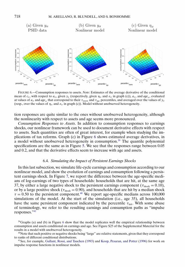
The empirical estimates below suggest that conditional skewness is a feature of the earn-ings process.

Preliminary Evidence on Nonlinear Persistence. Suggestive evidence of nonlinearity inthe persistence of earnings can be seen from Figure 1. This figure plots estimates of theaverage derivative, with respect to last period income yi!t−1, of the conditional quantilefunction of current income yit given yi!t−1. This average derivative effect is a measureof persistence analogous to ρt in (4), except that here we use residuals yit of log pre-taxhousehold labor earnings on a set of demographics (including education and a polynomialin the age of the household head) as outcome variables. Given the nature of the PSIDsample, panel (a) features biennial persistence estimates. On the two horizontal axes, wereport the percentile of yi!t−1 (“τinit”), and the percentile of the innovation of the quantileprocess (“τshock”). For estimation, we use a series quantile specification, as in (5), basedon a third-order Hermite polynomial.

This simple descriptive analysis not only shows the similarity in the patterns of thenonlinearity of household earnings in both the PSID household panel survey data and

14Similarly, a measure of conditional kurtosis is, for some α< 1 − τ,

kurt(ηi!t−1! τ!α)= Qt(ηi!t−1!1 − α)−Qt(ηi!t−1!α)

Qt(ηi!t−1! τ)−Qt(ηi!t−1!1 − τ) "


in the annual population register data from Norway; it also suggests differences in theimpact of an innovation to the quantile process (τshock) according to both the directionand magnitude of τshock and the percentile of the past level of income τinit. Persistenceof earnings history is highest when high-earnings households (i.e., high τinit) are hit by agood shock (high τshock), and when low-earnings households (i.e., low τinit) are hit by a badshock (low τshock). In both cases, estimated persistence is close to 0.9–1. In contrast, badshocks hitting high-earnings households, and good shocks hitting low-earnings ones, areassociated with much lower persistence of earnings history, as low as 0.3–0.4. In Section 6,we will see that our nonlinear model that separates transitory shocks from the persistentcomponent reproduces the nonlinear persistence patterns of Figure 1 for the PSID panelsurvey data and the Norwegian population register data.

3. MODEL (II): CONSUMPTION RULE

In order to motivate our empirical specification of the consumption function, we startby describing a standard stochastic life-cycle consumption model. We then use this setupto derive the form of the policy rule for household consumption, and describe the empir-ical consumption model that we will take to the data.

3.1. The Consumption Rule in a Simple Life-Cycle Model

We consider a theoretical framework where households act as single agents. Through-out their lifetime, households have access to a single risk-free, one-period bond whoseconstant return is 1 + r, and, at age t, face a period-to-period budget constraint

Ait = (1 + r)Ai!t−1 +Yi!t−1 −Ci!t−1! (7)

where Ait , Yit , and Cit denote assets, income, and consumption, respectively. Family log-earnings are given by lnYit = κt +ηit + εit , where κt is a deterministic age profile, and ηit

and εit are persistent and transitory earnings components, respectively. At age t, agentsknow ηit , εit and their past values, but not ηi!t+1 or εi!t+1, so there is no advance informa-tion. All distributions are known to households, and there is no aggregate uncertainty. Ineach period t in the life-cycle, the optimization problem is represented by the Bellmanequation

Vt(Ait!ηit! εit)= maxCit

u(Cit)+βEt

[Vt+1(Ai!t+1!ηi!t+1! εi!t+1)

]! (8)

where u(·) is agents’ utility, and β is the discount factor. An important element in (8) isthe conditional distribution of the Markov component ηi!t+1 given ηit , which enters theexpectation.

In a nonlinear earnings model such as (1)–(2), the presence of “unusual” shocks toearnings may lead to precautionary motives that induce high-income households to savemore than they would do under a linear earnings model. Even with certainty equiva-lent preferences, under model (1)–(2) the discounting applied to persistent shocks will bestate-dependent. In Section S1 of the Supplemental Material, we illustrate these theoret-ical mechanisms in a two-period version of the model. In Section S2, we report the resultsof a simulation exercise based on the life-cycle model. We compare the canonical linearearnings model with an earnings model that features the presence of positive and negative“unusual” shocks. In the simulated economy, we find that an implication of the nonlinear


earnings process is to reduce consumption among households on higher incomes. In par-ticular, a negative shock for those on higher incomes reduces the persistence of the pastand consequently is more damaging in terms of expected future incomes, thus inducinghigher saving, higher wealth accumulation, and lower consumption.15

In such a life-cycle model with uncertainty, the consumption rule will have the form

Cit = Gt(Ait!ηit! εit)! (9)

for some age-dependent function Gt . We will base our empirical specification on (9). Theconsumption rule at age t will be of this nonparametric form where the state variables att are period-t assets and the latent earnings components.16

In documenting dynamic patterns of consumption and earnings, one strategy is to takea stand on the functional form of the utility function and the distributions of the shocks,and to calibrate or estimate the model’s parameters by comparing the model’s predic-tions with the data. Another strategy is to linearize the Euler equation, with the help ofthe budget constraint; with a linear approximated problem at hand, standard covariance-based methods may be used for estimation. Our approach differs from those strategiesas we directly estimate the nonlinear consumption rule (9). Doing so, we avoid linearizedfirst-order conditions, and we estimate a flexible rule that is consistent with the abovelife-cycle consumption model. This approach allows documenting a rich set of derivativeeffects, thus shedding light on the patterns of consumption responses in the data.

3.2. Empirical Consumption Rule

Consider a cohort of households. Let cit denote log-consumption net of age dummies.Similarly, let ait denote log-assets net of age dummies. Our empirical specifications arebased on

cit = gt(ait!ηit! εit! νit)! t = 1! " " " !T" (10)

The νit are unobserved arguments of the consumption function, in addition to assets andthe latent earnings components. In the specification without unobserved individual het-erogeneity, νit are independent across periods and independent of (ait!ηit! εit), and gt

is monotone in ν. An economic interpretation for ν is as a taste shifter that increasesmarginal utility. In the single-asset life-cycle model of Section 3.1, monotonicity is impliedby the Bellman equation, provided ∂u(C!ν′)

∂C> ∂u(C!ν)

∂Cfor all C if ν′ > ν, where the house-

hold’s utility function is u(C! ν). Without loss of generality, we normalize the marginaldistribution of νit to be standard uniform in each period. From an empirical perspective,the presence of the taste shifters νit in the consumption rule (10) may also partly capturemeasurement error in consumption expenditures. In the specification with unobservedindividual heterogeneity, νit comprises two components: a time-invariant latent house-hold factor, and an i.i.d. uniform component independent of the latter. Consumption ismonotone in the second component, while being fully nonlinear in the first.

15In addition, in Section S2 of the Supplemental Material, we report simulation results based on the samelife-cycle model, using as input the earnings process we estimate on the PSID.

16Our approach may be extended to allow for habits or advance information, through simple modificationsof the vector of state variables. There could also be additional borrowing constraints in each period. In thatcase, the nonparametric consumption rule in (9) would no longer be differentiable. The derivative effectsdefined below require differentiability of gt .


Clearly, the net assets variable ait is not exogenous. In order to ensure identification,it suffices to specify ait as sequentially exogenous (or “predetermined”). We will spec-ify assets as a function of lagged assets, consumption, earnings, the persistent earningscomponent η, and age, as follows:

ait = ht(ai!t−1! ci!t−1! yi!t−1!ηi!t−1!υit)! (11)

where ht is an age-specific function which is increasing in its last argument, and υit arei.i.d. uniform independent of the other arguments. Note that the standard linear asset rule(7) is a special case of (11), so imposing (7) is not needed for identification or estimation.Taking a stand on the budget constraint will, however, be required in order to simulatethe impact of earnings shocks over the life-cycle.

Derivative Effects. Average consumption, for given values of asset holdings and earningscomponents, is

E[cit|ait = a!ηit = η!εit = ε] = E[gt(a!η!ε! νit)

]"

Our framework allows us to document how average consumption varies as a function ofassets and the two earnings components, and over the life-cycle. In particular, the averagederivative of consumption with respect to η is

φt(a!η!ε) = E[∂gt(a!η!ε! νit)

∂η

]" (12)

The parameter φt(a!η!ε) reflects the degree of insurability of shocks to the persistentearnings component.17 We will document how this new measure of partial insurance variesover the life-cycle, and how it depends on households’ asset holdings, by reporting esti-mates of the average derivative effect φt(a)= E[φt(a!ηit! εit)]. The quantity 1 −φt(a) isthen a general measure of the degree of consumption insurability of shocks to the persis-tent earnings component, as a function of age and assets.

Dynamic Effects of Earnings Shocks on Consumption. Other measures of interest arethe effects of an earnings shock uit to the η component on the consumption profile ci!t+s,s ≥ 0. For example, the contemporaneous effect can be computed, using the chain ruleand equation (12), as

E[∂

∂u

∣∣∣∣u=τ

gt

(a!Qt(η!u)! ε! νit

)]=φt

(a!Qt(η!τ)! ε

)∂Qt(η!τ)

∂u"

This derivative effect depends on η through the insurance coefficient φt , but also throughthe quantity ∂Qt(η!τ)

∂uas the earnings model allows for general forms of conditional het-

eroscedasticity and skewness. The quantity ∂Qt(η!τ)∂u

measures the responsiveness of earn-ings to a shock uit on impact. Note that its derivative with respect to η is equal to ∂ρt (η!τ)

∂τ,

where ρt(η!τ) is our persistence measure. In the empirical analysis, we will report finite-difference counterparts to these derivative effects (“impulse responses”), and find anasymmetric impact of earnings shocks at different points of the income distribution.

Multiple Assets. Our approach can be generalized to represent the consumption pol-icy function of a model with multiple assets differing in the stochastic properties of theirreturns. An example is a model that distinguishes between a risky asset and a risk-free

17Likewise, the average derivative with respect to ε is ψt (a!η!ε) = E[ ∂gt (a!η!ε!νit )∂ε

].


asset, as often used in studies of household portfolios (e.g., Alan (2012)). A version of theconsumption rule (10) with two assets would be consistent with this type of model as longas excess returns of the risky asset are not heterogeneous across households. In the pres-ence of kinks induced by participation or transaction costs, our empirical consumptionrule would capture a smoothed approximation.

The consumption rule (10) can also be extended to the Kaplan and Violante (2014)model of wealthy “hand-to-mouth” consumers. In that framework, the consumption pol-icy rule is a nonlinear function of assets disaggregated into liquid and illiquid parts. Ac-cess to the illiquid, higher return asset involves a transaction cost. The separate assetsinteract in nonlinear ways with earnings. In this dynamic choice environment, the nonlin-earity in the consumption model (10) incorporating the two separate assets can providea smoothed approximation to the complex paths involved in the Kaplan and Violante(2014) composite consumption function.18

4. IDENTIFICATION

The earnings and consumption models take the form of nonlinear state-space models.A series of recent papers (notably Hu and Schennach (2008), and Hu and Shum (2012))has established conditions under which nonlinear models with latent variables are non-parametrically identified under conditional independence restrictions. Techniques devel-oped in this literature can be used in order to establish identification of the models weconsider.

4.1. Earnings Process

Consider model (1)–(2), where ηit is a Markovian persistent component and εit areindependent over time and independent of the η’s. We assume that the data contain Tconsecutive periods, t = 1! " " " !T . So, for a given cohort of households, t = 1 correspondsto the age at which the household head enters the sample, and t = T corresponds to thelast period of observation.19 For that cohort, our aim is to identify the joint distributionsof (ηi1! " " " !ηiT ) and (εi1! " " " ! εiT ) given i.i.d. data from (yi1! " " " ! yiT ). Four periods areneeded in order to identify at least one Markov transition Qt .

Conditions for the nonparametric identification of the earnings process are direct con-sequences of the analysis in Hu and Schennach (2008) and Wilhelm (2015). We providesuch conditions in Appendix A. Identification is derived under several high-level assump-tions. In particular, the distributions of (yit |yi!t−1) and (ηit |yi!t−1) both need to satisfy com-pleteness conditions. For example, the first condition requires that the only function h(in a suitable functional space) satisfying E[h(yit)|yi!t−1] = 0 be h = 0. This requires thatηi!t−1 and ηit be statistically dependent, albeit without specifying the form of that depen-dence. An intuition for this is that if η’s were independent over time, there would be noway to distinguish them from the transitory ε’s. Completeness is commonly assumed innonparametric instrumental variables problems (Newey and Powell (2003)).

18A separate question of interest, but one that is beyond the scope of this paper, concerns the identificationof the latent consumption policy functions associated with the agent’s accessing or not accessing the illiquidasset. Such a question could be posed if we observed a time-varying indicator of whether or not consumersaccess their illiquid assets.

19We consider a balanced panel for simplicity, but our arguments can be extended to unbalanced panels.


4.2. Consumption Rule

Let us now turn to the identification of the consumption rule (10), starting with the casewithout unobserved heterogeneity. We make the following assumptions, where we denotezti = (zi1! " " " !zit).

ASSUMPTION 1: For all t ≥ 1,(i) ui!t+s and εi!t+s, for all s ≥ 0, are independent of at

i , ηt−1i , and yt−1

i . εi1 is independentof ai1 and ηi1.

(ii) ai!t+1 is independent of (at−1i ! ct−1

i ! yt−1i !ηt−1

i ) conditional on (ait! cit! yit!ηit).(iii) The taste shifter νit in (10) is independent of ηi1, (uis! εis) for all s, νis for all s = t,

and ati .

Part (i) in Assumption 1 requires current and future earnings shocks, which are in-dependent of past components of earnings, to be independent of current and past assetholdings as well. At the same time, we let ηi1 and ai1 be arbitrarily dependent. This is im-portant, because asset accumulation upon entry in the sample may be correlated with pastearnings shocks. Part (ii) is a first-order Markov condition on asset accumulation. It is sat-isfied in a standard life-cycle model with one single risk-less asset; see equation (7). Theassumption also holds in such a model when the interest rate rt is time-varying and knownto households. More generally, the assumption allows the latent components of earningsηit and εit to affect asset holdings separately, as in (11). Last, part (iii) requires tasteshifters to be independent over time, independent of earnings components, and indepen-dent of current and past assets. In particular, this rules out the presence of unobservedheterogeneity in consumption. We will relax this condition in the next subsection.

The identification argument proceeds in a sequential way. Starting with the first period,letting yi = (yi1! " " " ! yiT ), and using f as a generic notation for a density function, we have

f (a1|y)=∫

f (a1|η1)f (η1|y)dη1! (13)

where we have used that, by Assumption 1(i), f (a1|η1! y) and f (a1|η1) coincide. We canrewrite (13) as

f (a1|y)= E[f (a1|ηi1)|yi = y

]! (14)

where the expectation is taken with respect to the density of ηi1 given yi, for a fixedvalue a1. Hence, provided the distribution of (ηi1|yi) (which is identified from the earn-ings process; see above) is complete, the density f (a1|η1) is identified from (14).20 Notethat the density f (a1!η1|y)= f (a1|η1)f (η1|y) is also identified.

We then have, using the consumption rule and Assumption 1(iii),

f (c1|a1! y)=∫

f (c1|a1!η1! y1)f (η1|a1! y)dη1! (15)

or equivalently,

f (c1|a1! y)= E[f (c1|ai1!ηi1! yi1)|ai1 = a1! yi = y

]! (16)

20In fact, given that we are working with bounded density functions, it is sufficient that the distribution of(ηi1|yi) be boundedly complete; see Blundell, Chen, and Kristensen (2007) for analysis and discussion.


where the conditional expectation is taken at fixed c1. Under completeness in (yi2! " " " ! yiT )of the distribution of (ηi1|ai1! yi) (which is identified from the previous paragraph),21 thedensities f (c1|a1!η1! y1) and f (c1!η1|a1! y) are thus identified. Identification of the con-sumption function (10) for t = 1 follows since g1 is the conditional quantile function of c1

given a1, η1, and ε1 = y1 −η1.Second Period’s Assets. Turning to period 2, we have, using Assumption 1(i) and (iii),

f (a2|c1!a1! y)=∫

f (a2|c1!a1!η1! y1)f (η1|c1!a1! y)dη1! (17)

from which it follows that the density f (a2|c1!a1!η1! y1) is identified, provided the distri-bution of (ηi1|ci1!ai1! yi) (which is identified from above) is complete in (yi2! " " " ! yiT ).

In addition, using Bayes’s rule and Assumption 1(i) and (iii),

f (η2|a2! c1!a1! y) =∫

f (y|η1!η2! y1)f (η1!η2|a2! c1!a1! y1)

f (y|a2! c1!a1! y1)dη1"

So, as the density f (η1|a2! c1!a1! y1) is identified from above, and by Assumption 1

f (η1!η2|a2! c1!a1! y1)= f (η1|a2! c1!a1! y1)f (η2|η1)!

it follows that f (η2|a2! c1!a1! y) is identified.Subsequent Periods. To see how the argument extends to subsequent periods, consider

second period’s consumption. We have, using Assumption 1(iii),

f (c2|a2! c1!a1! y)=∫

f (c2|a2!η2! y2)f (η2|a2! c1!a1! y)dη2" (18)

Provided the distribution of (ηi2|ai2! ci1!ai1! yi) (which is identified from the previousparagraph) is complete in (ci1!ai1! yi1! yi3! " " " ! yiT ), the density f (c2|a2!η2! y2) is identi-fied.

By induction, using in addition Assumption 1(ii) from the third period onward,the joint density of η’s, consumption, assets, and earnings is identified provided,for all t ≥ 1, the distributions of (ηit |cti !at

i! yi) and (ηit |ct−1i !at

i! yi) are complete in(ct−1

i !at−1i ! yt−1

i ! yi!t+1! " " " ! yiT ).Discussion. The identification arguments depend on completeness conditions, which re-

late to the relevance, in a nonparametric sense, of the instruments. To illustrate this, con-sider the completeness of the distribution of (ηi1|yi) in (yi2! " " " ! yiT ), which we use to showthe identification of the consumption rule in the first period; see (16). Here we abstractfrom assets for simplicity. The completeness condition then depends on the propertiesof the earnings process. As an example, consider the case where T = 2, and (ηi1! yi1! yi2)follows a multivariate normal distribution with zero mean. Then ηi1 = αyi1 + βyi2 + ζi,where ζi is normal (0!σ2), independent of (yi1! yi2). It can be easily shown that β = 0 ifCov(ηi1!ηi2) = 0, in which case the distribution of (ηi1|yi1! yi2) is complete in yi2. As inthe identification of the earnings process, identification of the consumption rule thus re-lies on η’s being dependent over time. Beyond the settings studied so far in the literature

21Here, by completeness in yi2 of the distribution of (yi1|yi2!xi) we mean that the only solution toE[h(yi1!xi)|yi2!xi] = 0 is h = 0. This is the same as (yi1!xi)|(yi2!xi) being complete. Note that, similarly asbefore, the weaker condition of bounded completeness suffices.


(such as in D’Haultfoeuille (2011), Andrews (2011), or Hu and Shiu (2012)), it would beof great interest to provide primitive conditions for completeness in the nonlinear modelswe focus on here.

An intuitive explanation for the identification argument comes from the link to non-parametric instrumental variables (NPIV). In period 1, for a fixed a1, (14) is analogousto an NPIV problem where ηi1 is the endogenous regressor and yi = (yi1! " " " ! yiT ) is thevector of instruments. Likewise, conditional on (ai1! yi1), (yi2! " " " ! yiT ) are the “excludedinstruments” for ηi1 in (16). In subsequent periods, lagged consumption and assets areused as instruments, together with lags and leads of earnings. Using leads of log-earningsfor identifying consumption responses is a common strategy in linear models; see, forexample, Hall and Mishkin (1982) and Blundell, Pistaferri, and Preston (2008).

4.3. Household Unobserved Heterogeneity

Accounting for unobserved heterogeneity in preferences or discounting, for example,may be empirically important. Heterogeneity in discount factors is also a popular mech-anism in quantitative macroeconomic models to generate realistic wealth inequality; see,for example, Krusell and Smith (1998) and Krueger, Mitman, and Perri (2015). With un-observed heterogeneity, the consumption rule takes the form

cit = gt(ait!ηit! εit! ξi! νit)! t = 1! " " " !T! (19)

where ξi is a household-specific effect and νit are i.i.d. standard uniform. The distributionof (ξi!ηi1!ai1) is left unrestricted. Therefore, ξi is treated as a “fixed effect.” Even if afully unstructured distinction between unobserved heterogeneity and individual dynamicsin a finite horizon panel is not possible, finite-dimensional fixed effects can be includednonparametrically in the consumption (and earnings) equations as long as T is sufficientlylarge. In Appendix A, we provide conditions for identification of this model, by relying onresults from Hu and Schennach (2008). For simplicity, we consider scalar heterogeneity ξi.Depending on the number of available time periods, a vector of unobserved heterogeneitycould be allowed for.

Last, in Section S3 of the Supplemental Material, we consider several extensions ofthe model. We show how to allow for unobserved heterogeneity in earnings, as in thefollowing specification that we will take to the data:

yit = ηit + ζi + εit! (20)

where ηit = Qt(ηi!t−1!uit) is first-order Markov. We also describe how to allow for depen-dence in transitory shocks, advance earnings information, and consumption habits.

5. ESTIMATION STRATEGY

5.1. Empirical Specification

Earnings Components. The earnings model depends on the Markovian transitions of thepersistent component Qt(·! ·), the marginal distributions of εit , and the marginal distribu-tion of the initial persistent component ηi1. We now explain how we empirically specifythese three components.


Let ϕk, for k = 0!1! " " " , denote a dictionary of bivariate functions, with ϕ0 = 1. Lettingageit denote the age of the head of household i in period t, we specify

Qt(ηi!t−1! τ) = Q(ηi!t−1!ageit! τ)(21)

=K∑

k=0

aQk (τ)ϕk(ηi!t−1!ageit)"

In practice, we use low-order products of Hermite polynomials for ϕk. We specify thequantile function of εit (for t = 1! " " " !T ) given ageit , and that of ηi1 given age at the startof the period agei1, in a similar way. Specifically, we set

Qε(ageit! τ) =K∑

k=0

aεk(τ)ϕk(ageit)!

Qη1(agei1! τ) =K∑

k=0

aη1k (τ)ϕk(agei1)!

with outcome-specific choices for K and ϕk.The quantile model (21) provides a flexible specification of the conditional distribution

of ηit given ηi!t−1 and age. Similarly, our quantile specifications flexibly model how εitand ηi1 depend on age, at every quantile. We include the age of the household head asa control, while ruling out dependence on calendar time. This choice is motivated by ourdesire to model life-cycle evolution, as well as by the relative stationarity of the earningsdistributions (conditional on age) during the 1999–2009 period and the relatively smallsample size. On larger samples, an interesting avenue will be to allow for variation inboth age and calendar time within our framework.22

Consumption Rule. Following from Section 3.2, we specify the conditional distributionof consumption given current assets and earnings components as follows:

gt(ait!ηit! εit! τ) = g(ait!ηit! εit!ageit! τ)(22)

=K∑

k=1

bgkϕk(ait!ηit! εit!ageit)+ bg

0(τ)!

where ϕk is a dictionary of functions (in practice, another product of Hermite polynomi-als).

Equation (22) is a nonlinear regression model. In contrast with (21), the consumptionmodel is additive in τ. It would be conceptually straightforward to let all coefficients bg

k

depend on τ, although this would lead to a less parsimonious specification. Below weaugment the consumption function to also depend nonlinearly on a household-specificeffect.

22The functional form in (21) does not enforce monotonicity in τ, but our estimation method will producean automatic rearrangement of quantiles if needed.


Assets Evolution. We specify the distribution of initial assets ai1 conditional on the initialpersistent component ηi1 and the age at the start of the period agei1 as

Qa(ηi1!agei1! τ)=K∑

k=0

bak(τ)ϕk(ηi1!agei1)! (23)

for different choices for K and ϕk. We then specify how assets evolve as a function oflagged assets, consumption, earnings, the persistent earnings component η, and age, using(11), where

ht(ai!t−1! ci!t−1! yi!t−1!ηi!t−1! τ) = h(ai!t−1! ci!t−1! yi!t−1!ηi!t−1!ageit! τ)(24)

=K∑

k=1

bhkϕk(ai!t−1! ci!t−1! yi!t−1!ηi!t−1!ageit)+ bh

0(τ)!

for some K and ϕk.23

Implementation. The functions aQk , aεk, and aη1

k are indexed by a finite-dimensional pa-rameter vector θ. Likewise, the functions bg

0 , bh0 , and ba

k are indexed by a parameter vec-tor µ that also contains bg

1! " " " !bgK!b

h1 ! " " " !b

hK . We base our implementation on Wei and

Carroll (2009) and Arellano and Bonhomme (2016). As in these papers, we model thefunctions aQ

k as piecewise-polynomial interpolating splines on a grid [τ1! τ2], [τ2! τ3], . . . ,[τL−1! τL], contained in the unit interval. We extend the specification of the intercept co-efficient aQ

0 on (0! τ1] and [τL!1) using a parametric model indexed by λQ. All aQk for

k ≥ 1 are constant on [0! τ1] and [τL!1], respectively. Hence, denoting aQkℓ = aQ

k (τℓ), thefunctions aQ

k depend on {aQ11! " " " !a

QKL!λ

Q}.Unlike in an ordinary quantile regression, the dependence of the parameters on the

percentiles τ needs to be specified because some of our regressors are latent variables. Inpractice, we take L = 11 and τℓ = ℓ/(L + 1). The functions aQ

k are taken as piecewise-linear on [τ1! τL]. An advantage of this specification is that the likelihood function isavailable in closed form. In addition, we specify aQ

0 as the quantile of an exponentialdistribution on (0! τ1] (with parameter λQ

−) and [τL!1) (with parameter λQ+).24

We proceed similarly to model aεk, aη1k , and ba

k. Moreover, as our data show little evi-dence against consumption being log-normal, we set bg

0(τ) to α+ σ+−1(τ), where (α!σ)are parameters to be estimated. We proceed similarly for bh

0(τ). We also estimated twodifferent versions of the model with more flexible specifications for bg

0(τ) and bh0(τ): based

on quantiles on a grid with L = 11 knots, and allowing for an age effect in the varianceof the consumption innovation. In both cases, we found very similar results to the ones

23In a previous version of the paper, we estimated the model imposing thatηi!t−1 does not enter (24), which isstill consistent with the budget constraint (7) and avoids the need to model predetermined assets. We obtainedqualitatively similar empirical results.

24As a result, we have

aQ0 (τ) = 1

λQ−

log(τ

τ1

)1{0 < τ < τ1} +

L−1∑

ℓ=1

(aQkℓ +

aQk!ℓ+1 − aQ

kℓ

τℓ+1 − τℓ(τ− τℓ)

)1{τℓ ≤ τ < τℓ+1}

− 1λQ

+log

(1 − τ1 − τL

)1{τL ≤ τ < 1}"


we report below. We use tensor products of Hermite polynomials for ϕk and ϕk, eachcomponent of the product taking as argument a standardized variable.25

Household Unobserved Heterogeneity. When allowing for household unobserved hetero-geneity in consumption/assets, we model log-consumption as

cit = g(ait!ηit! εit!ageit! ξi! νit)! (25)

which we specify similarly as in (22), with parameters bgk. To fix the scale of the function,

we impose thatK∑

k=1

bgkϕk(0!0!0!age! ξ)= ξ for all ξ! (26)

where age denotes the mean value of age in the sample. Likewise, we model assets as

ait = h(ai!t−1! ci!t−1! yi!t−1!ηi!t−1!ageit! ξi! υit)! (27)

with a similar specification as in (24). Last, we specify ξi = q(ai1!ηi1!agei1!ωi), with ωi

uniform on (0!1), using a quantile modeling as in (23).26

5.2. Overview of the Estimation Algorithm

The algorithm is an adaptation of techniques developed in Arellano and Bonhomme(2016) to a setting with time-varying latent variables. The first estimation step recovers es-timates of the earnings parameters θ. The second step recovers estimates of the consump-tion and assets parameters µ, given a previous estimate of θ. Our choice of a sequentialestimation strategy, rather than joint estimation of (θ!µ), is motivated by the fact that θis identified from the earnings process alone. In contrast, in a joint estimation approach,estimates of the earnings process would be partly driven by the consumption model. Herewe describe the estimation of the earnings parameters θ. Estimation of the consumptionparameters µ is similar. The model’s restrictions are described in detail in Appendix B.

A compact notation for the restrictions implied by the earnings model is

θ= argminθ

E[∫

R(yi!η;θ)fi(η;θ)dη]!

where R is a known function, θ denotes the true value of θ, and fi(·;θ) = f (·|yTi !ageTi ;θ)

denotes the posterior density of (ηi1! " " " !ηiT ) given the earnings data. The estimation al-gorithm is closely related to the “stochastic EM” algorithm (Celeux and Diebolt (1993)).Stochastic EM is a simulated version of the classical EM algorithm of Dempster, Laird,and Rubin (1977), where new draws from η are computed in every iteration of the algo-rithm. One difference is that, unlike in EM, our problem is not likelihood-based. Instead,we exploit the computational convenience of quantile regression and replace likelihoodmaximization by a sequence of quantile regressions in each M-step of the algorithm.

Starting with a parameter vector θ(0), we iterate the following two steps on s = 0!1!2! " " "until convergence of the θ(s) process:

25For example, at/std(a), ηt /std(y), εt/std(y), and (aget − mean(age))/std(age) are used as arguments ofthe consumption rule.

26We proceed analogously when allowing for an additive household-specific effect ζi in log-earnings yit =ηit + ζi + εit , where ηit is given by (2). There we allow for flexible dependence between ηi1, ζi , and agei1through another series quantile model.


1. Stochastic E-step: Draw η(m)i = (η(m)

i1 ! " " " !η(m)iT ) for m= 1! " " " !M from fi(·; θ(s)).

2. M-step: Compute

θ(s+1) = argminθ

N∑

i=1

M∑

m=1

R(yi!η

(m)i ;θ

)"

Note that, as the likelihood function is available in closed form, the E-step is straightfor-ward. In practice, we use a random-walk Metropolis–Hastings sampler for this purpose,targeting an acceptance rate of approximately 30%. The M-step consists of a number ofquantile regressions. For example, the parameters aQ

kℓ are updated as

min(aQ0ℓ!"""!a

QKℓ)

N∑

i=1

T∑

t=2

M∑

m=1

ρτℓ

(

η(m)it −

K∑

k=0

aQkℓϕk

(η(m)

i!t−1!ageit))

! ℓ= 1! " " " !L!

where ρτ(u) = u(τ − 1{u ≤ 0}) is the “check” function. This is a set of standard quantileregressions, associated with convex objective functions. We proceed in a similar way toupdate all other parameters; see Appendix B for details.

In practice, we first estimate the effect of age on mean log-earnings by regressing themon a quartic in age. We then impose in each iteration of the algorithm that εit and ageare uncorrelated (although we allow for age effects on the variance and quantiles of εit).We take M = 1, stop the chain after a large number of iterations, and report an averageacross the last S values θ= 1

S

∑Ss=S−S+1 θ

(s), and similarly for consumption-related parame-ters µ.27 The results for the earnings parameters are based on S = 500 iterations, with 200Metropolis–Hastings draws in each iteration. Consumption-related parameters are esti-mated using 200 iterations with 200 draws per iteration. In both cases, we take S = S/2. Inour experiments, we observed that the algorithm may get “stuck” on what appears to be alocal regime of the Markov chain. We started the algorithm from a large number of initialparameter values, and selected the estimates yielding the highest average log-likelihoodover iterations. The non-selected values tended to give very similar pictures to the oneswe report below.

Properties. Nielsen (2000) studied the statistical properties of the stochastic EM algo-rithm in a likelihood case. He provided conditions under which the Markov chain θ(s) isergodic, for a fixed sample size. He also characterized the asymptotic distribution of θas the sample size N tends to infinity. Arellano and Bonhomme (2016) characterized theasymptotic distribution of θ in a case where the optimization step is not likelihood-basedbut relies on quantile-based estimating equations. The estimator θ is root-N consistentand asymptotically normal under correct specification of the parametric model, for K andL fixed. Note that an alternative, nonparametric approach would be to let K and L in-crease with N at an appropriate rate so as to let the approximation bias tend to zero.28

Studying inference in our problem as (N!K!L) jointly tend to infinity is an interestingavenue for future work.

27As an alternative to taking a large M , taking M = 1 and averaging the parameter draws is computationallyconvenient in our setting.

28See Belloni, Chernozhukov, Chetverikov, and Fernández-Val (2016) for an analysis of inference for seriesquantile regression, and Arellano and Bonhomme (2016) for a consistency analysis in a panel data modelclosely related to the one we consider here.


6. EMPIRICAL RESULTS ON EARNINGS AND CONSUMPTION

In this section, we present our empirical results. We start by describing our main datasource, the Panel Study of Income Dynamics (PSID). We then show how earnings andconsumption respond to income shocks. We also corroborate our findings for the nonlin-ear earnings process using administrative data on household earnings from the Norwegianpopulation register. Finally, we report simulation exercises based on the estimated model.

6.1. Panel Data

Panel data on household consumption, income, and assets are rare. The PSID beganthe collection of detailed data on consumption expenditures and asset holdings in 1999,in addition to household earnings and demographics. An annual wave is available everyother year. We use data for the 1999–2009 period (six waves).

Earnings Yit are total pre-tax household labor earnings. We construct yit as residualsfrom regressing log household earnings on a set of demographics, which include cohortinteracted with education categories for both household members, race, state, and large-city dummies, a family size indicator, number of kids, a dummy for income recipient otherthan husband and wife, and a dummy for kids out of the household. Controls for familysize and composition are included so as to equivalize household earnings (likewise forconsumption and assets below). Education, race, and geographic dummies are includedin an attempt to capture individual heterogeneity beyond cohort effects and the initialpersistent component of earnings ηi1. Removing demographic-specific means in a prelim-inary step has been the standard practice in the empirical analysis of earnings dynamics.A more satisfactory approach would integrate both steps, especially given our emphasison nonlinearities. However, except for age, we did not attempt a richer conditioning inlight of sample size.

We use data on consumption Cit of nondurables and services. The panel data containinformation on health expenditures, utilities, car-related expenditures and transportation,education, child care, and food expenditures. Recreation, alcohol, tobacco, and clothing(the latter available from 2005) are the main missing items. Rent information is availablefor renters, but not for home owners. We follow Blundell, Pistaferri, and Saporta-Eksten(2016) and impute rent expenditures for home owners.29 In total, approximately 67% ofconsumption expenditures on nondurables and services are covered. We construct cit asresiduals of log total consumption on the same set of demographics as for earnings.

Asset holdings Ait are constructed as the sum of financial assets (including cash, stocks,and bonds), real estate value, pension funds, and car value, net of mortgages and otherdebt. We construct residuals ait by regressing log-assets on the same set of demographicsas for earnings and consumption. These log-assets residuals will enter as arguments of thenonlinear consumption rule (10).

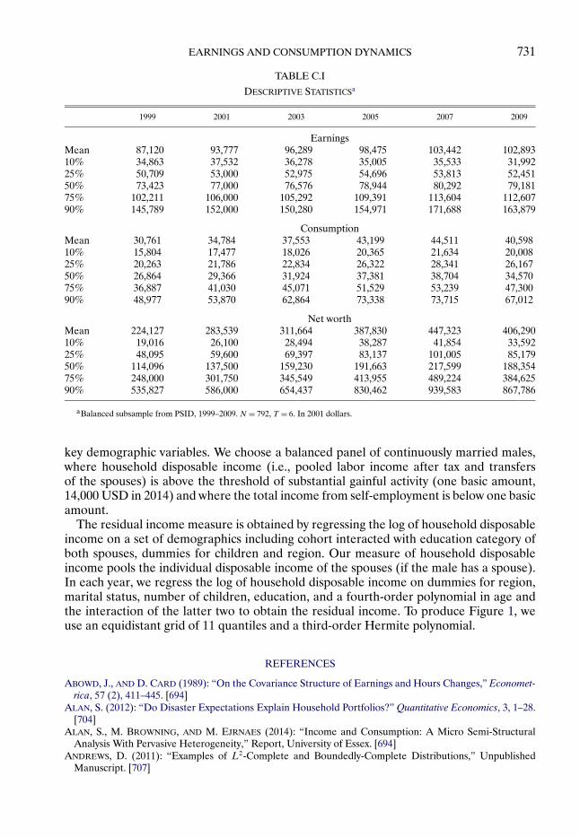
To select the sample, we follow Blundell, Pistaferri, and Saporta-Eksten (2016) and fo-cus on a sample of participating and married male heads aged between 25 and 60. Wedrop all observations for which data on earnings, consumption, or assets, either in levelsor log-residuals, are missing. See Appendix C for further details. In the analysis, we focuson a balanced subsample of N = 792 households. Table C.I in Appendix C shows meantotal earnings, consumption, and asset holdings, by year. Compared to Blundell, Pista-ferri, and Saporta-Eksten (2016), households in our balanced sample have higher assets,

29Note that, as a result, consumption responds automatically to variations in house prices. An alternativewould be to exclude rents and imputed rents from consumption expenditures.


and to a lesser extent higher earnings and consumption. The table also shows a large andincreasing dispersion of assets across households. The evolution of assets may partly re-flect the housing boom and bust, including the effect of the Great Recession at the end ofthe sample. Although our framework could be used to document distributional dynamicsalong the business-cycle, we abstract from business-cycle effects in this paper.

Last, the sample that we use is relatively homogeneous. Including households withless stable employment histories would be interesting, but it would require extending ourframework. We return to this point in the conclusion.

6.2. Earnings

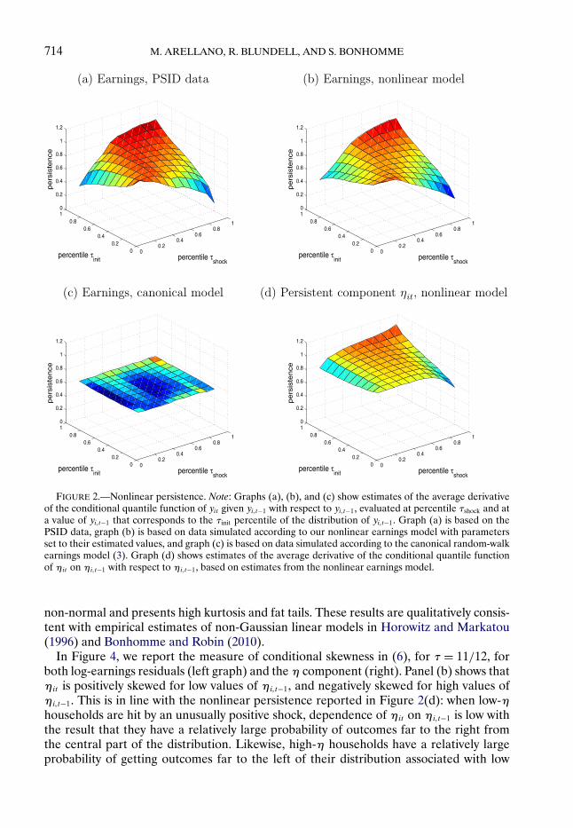
We next comment on the empirical estimates of the earnings process. Figure 2(a) repro-duces Figure 1(a). It shows estimates of the average derivative of the conditional quantilefunction of log-earnings residuals yit given yi!t−1 with respect to yi!t−1 in the PSID sam-ple. The figure suggests the presence of nonlinear persistence, which depends on boththe percentile of past income (τinit) and the percentile of the quantile innovation (τshock).This empirical pattern is also present for male wages; see Figure S1 of the SupplementalMaterial. We then estimate the earnings model,30 and, given the estimated parameters,we simulate the model.31 Figure 2(b), which is based on simulated data, shows that ournonlinear model reproduces the patterns of nonlinear persistence well. In contrast, stan-dard models have difficulty fitting this empirical pattern. For example, we estimated asimple version of the canonical earnings dynamics model (3) with a random-walk compo-nent and independent transitory shocks.32 Figure 2(c) shows that the average derivativeof the quantile function is nearly constant (up to simulation error) with respect to τshock

and τinit. This linear specification without interaction effects between earnings shocks andpast earnings components stands in contrast with the data.33

Figure 2(d) then shows the estimated persistence of the earnings component ηit . Specif-ically, the graph shows ρt(ηi!t−1! τ) from equation (4), evaluated at percentiles τinit andτshock and at the mean age in the sample (47"5 years).34 Persistence in η’s is higher thanpersistence in log-earnings residuals, consistently with the fact that Figure 2(d) is netof transitory shocks. Persistence is close to 1 for high-earnings households hit by goodshocks, and for low-earnings households hit by bad shocks. At the same time, persistenceis lower, down to 0.6–0.8, when bad shocks hit high-earnings households or good shockshit low-earnings ones.

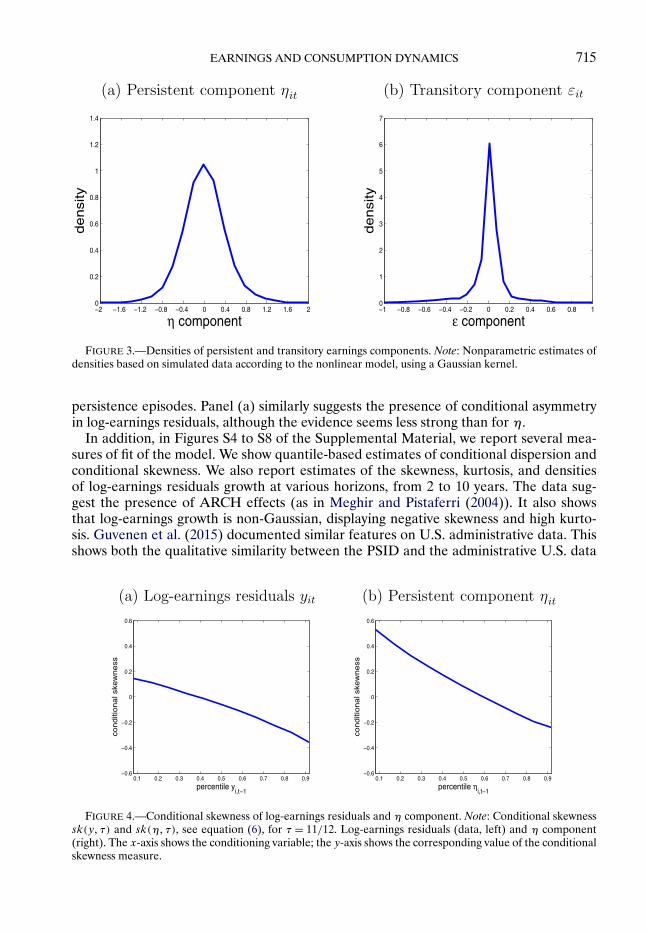
Densities and Moments. Figure 3 shows estimates of the marginal distributions of thepersistent and transitory earnings components at mean age. While the persistent compo-nent ηit shows relatively small departures from Gaussianity, the density of εit is clearly

30We use tensor products of Hermite polynomials of degrees (3!2) for the conditional quantile function ofηit given ηi!t−1 and age, and second-order polynomials for εit and ηi1 as a function of age.

31We draw 20 earnings values per household. In the simulation, we impose that the support of simulated ηdraws be less than three times the empirical support of log-earnings residuals. This affects very few observa-tions.

32Estimation is based on equally-weighted minimum distance using the covariance structure predicted bythe canonical model.

33In order to assess the sensitivity to the polynomial functional form that we use, in Figure S2 of the Sup-plemental Material, we report persistence estimates based on piecewise-linear specifications based on 9 or 25pieces. The characteristic shape of Figure 2(a) remains present.

34The estimated persistence is similar when averaging over age; see Figure S3 of the Supplemental Material.


FIGURE 2.—Nonlinear persistence. Note: Graphs (a), (b), and (c) show estimates of the average derivativeof the conditional quantile function of yit given yi!t−1 with respect to yi!t−1, evaluated at percentile τshock and ata value of yi!t−1 that corresponds to the τinit percentile of the distribution of yi!t−1. Graph (a) is based on thePSID data, graph (b) is based on data simulated according to our nonlinear earnings model with parametersset to their estimated values, and graph (c) is based on data simulated according to the canonical random-walkearnings model (3). Graph (d) shows estimates of the average derivative of the conditional quantile functionof ηit on ηi!t−1 with respect to ηi!t−1, based on estimates from the nonlinear earnings model.

non-normal and presents high kurtosis and fat tails. These results are qualitatively consis-tent with empirical estimates of non-Gaussian linear models in Horowitz and Markatou(1996) and Bonhomme and Robin (2010).

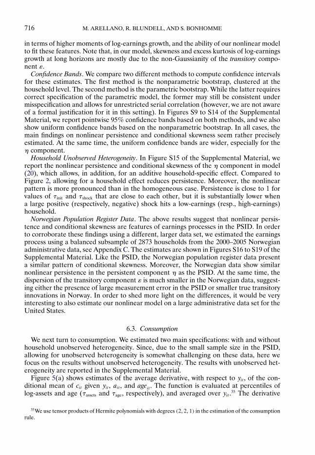
In Figure 4, we report the measure of conditional skewness in (6), for τ = 11/12, forboth log-earnings residuals (left graph) and the η component (right). Panel (b) shows thatηit is positively skewed for low values of ηi!t−1, and negatively skewed for high values ofηi!t−1. This is in line with the nonlinear persistence reported in Figure 2(d): when low-ηhouseholds are hit by an unusually positive shock, dependence of ηit on ηi!t−1 is low withthe result that they have a relatively large probability of outcomes far to the right fromthe central part of the distribution. Likewise, high-η households have a relatively largeprobability of getting outcomes far to the left of their distribution associated with low


FIGURE 3.—Densities of persistent and transitory earnings components. Note: Nonparametric estimates ofdensities based on simulated data according to the nonlinear model, using a Gaussian kernel.

persistence episodes. Panel (a) similarly suggests the presence of conditional asymmetryin log-earnings residuals, although the evidence seems less strong than for η.

In addition, in Figures S4 to S8 of the Supplemental Material, we report several mea-sures of fit of the model. We show quantile-based estimates of conditional dispersion andconditional skewness. We also report estimates of the skewness, kurtosis, and densitiesof log-earnings residuals growth at various horizons, from 2 to 10 years. The data sug-gest the presence of ARCH effects (as in Meghir and Pistaferri (2004)). It also showsthat log-earnings growth is non-Gaussian, displaying negative skewness and high kurto-sis. Guvenen et al. (2015) documented similar features on U.S. administrative data. Thisshows both the qualitative similarity between the PSID and the administrative U.S. data

FIGURE 4.—Conditional skewness of log-earnings residuals and η component. Note: Conditional skewnesssk(y! τ) and sk(η!τ), see equation (6), for τ = 11/12. Log-earnings residuals (data, left) and η component(right). The x-axis shows the conditioning variable; the y-axis shows the corresponding value of the conditionalskewness measure.


in terms of higher moments of log-earnings growth, and the ability of our nonlinear modelto fit these features. Note that, in our model, skewness and excess kurtosis of log-earningsgrowth at long horizons are mostly due to the non-Gaussianity of the transitory compo-nent ε.

Confidence Bands. We compare two different methods to compute confidence intervalsfor these estimates. The first method is the nonparametric bootstrap, clustered at thehousehold level. The second method is the parametric bootstrap. While the latter requirescorrect specification of the parametric model, the former may still be consistent undermisspecification and allows for unrestricted serial correlation (however, we are not awareof a formal justification for it in this setting). In Figures S9 to S14 of the SupplementalMaterial, we report pointwise 95% confidence bands based on both methods, and we alsoshow uniform confidence bands based on the nonparametric bootstrap. In all cases, themain findings on nonlinear persistence and conditional skewness seem rather preciselyestimated. At the same time, the uniform confidence bands are wider, especially for theη component.

Household Unobserved Heterogeneity. In Figure S15 of the Supplemental Material, wereport the nonlinear persistence and conditional skewness of the η component in model(20), which allows, in addition, for an additive household-specific effect. Compared toFigure 2, allowing for a household effect reduces persistence. Moreover, the nonlinearpattern is more pronounced than in the homogeneous case. Persistence is close to 1 forvalues of τinit and τshock that are close to each other, but it is substantially lower whena large positive (respectively, negative) shock hits a low-earnings (resp., high-earnings)household.

Norwegian Population Register Data. The above results suggest that nonlinear persis-tence and conditional skewness are features of earnings processes in the PSID. In orderto corroborate these findings using a different, larger data set, we estimated the earningsprocess using a balanced subsample of 2873 households from the 2000–2005 Norwegianadministrative data, see Appendix C. The estimates are shown in Figures S16 to S19 of theSupplemental Material. Like the PSID, the Norwegian population register data presenta similar pattern of conditional skewness. Moreover, the Norwegian data show similarnonlinear persistence in the persistent component η as the PSID. At the same time, thedispersion of the transitory component ε is much smaller in the Norwegian data, suggest-ing either the presence of large measurement error in the PSID or smaller true transitoryinnovations in Norway. In order to shed more light on the differences, it would be veryinteresting to also estimate our nonlinear model on a large administrative data set for theUnited States.

6.3. Consumption

We next turn to consumption. We estimated two main specifications: with and withouthousehold unobserved heterogeneity. Since, due to the small sample size in the PSID,allowing for unobserved heterogeneity is somewhat challenging on these data, here wefocus on the results without unobserved heterogeneity. The results with unobserved het-erogeneity are reported in the Supplemental Material.

Figure 5(a) shows estimates of the average derivative, with respect to yit , of the con-ditional mean of cit given yit , ait , and ageit . The function is evaluated at percentiles oflog-assets and age (τassets and τage, respectively), and averaged over yit .35 The derivative

35We use tensor products of Hermite polynomials with degrees (2!2!1) in the estimation of the consumptionrule.


FIGURE 5.—Consumption responses to earnings shocks, by assets and age, model without household-spe-cific unobserved heterogeneity. Note: Graphs (a) and (b) show estimates of the average derivative of the condi-tional mean of cit , with respect to yit , given yit , ait , and ageit , evaluated at values of ait and ageit that correspondto their τassets and τage percentiles, and averaged over the values of yit . Graph (a) is based on the PSID data, andgraph (b) is based on data simulated according to our nonlinear model with parameters set to their estimatedvalues. Graph (c) shows estimates of the average consumption responses φt (a) to variations in ηit , evaluatedat τassets and τage.

effects lie between 0.2 and 0.3. Moreover, the results indicate that consumption of olderhouseholds, and of households with higher assets, is less correlated to variations in earn-ings. Figure 5(b) shows the same response surface based on simulated data from our fullnonlinear model of earnings and consumption. The fit of the model, though not perfect,seems reasonable. In particular, the model reproduces the main pattern of correlationwith age and assets.36!37

Figure 5(c) shows estimates of the average consumption response φt(a) to variationsin the persistent component of earnings. As described in Section 3, 1 −φt(a) can be re-garded as a measure of the degree of consumption insurability of shocks to the persistentearnings component, as a function of age and assets. On average, the estimated φt(a)parameter lies between 0.3 and 0.4, suggesting that more than half of pre-tax householdearnings fluctuations is effectively insured. Moreover, variation in assets and age suggeststhe presence of an interaction effect. In particular, older households with high assets seembetter insured against earnings fluctuations.38

In Figures S22 and S23 of the Supplemental Material, we report 95% confidence bandsfor φt(a) based on both parametric bootstrap and nonparametric bootstrap. The findingson insurability of shocks to the persistent earnings component seem quite precisely es-timated. In Figure S24 of the Supplemental Material, we report estimates of the modelwith household unobserved heterogeneity in consumption; see (19). Estimated consump-

36In Figure S20 of the Supplemental Material, we show that the model fit to the density of log-consumptionis also good.

37While the covariances between log-earnings and log-consumption residuals are well reproduced, the base-line model does not perform as well in fitting the dynamics of consumption, as it systematically underestimatesthe autocorrelations between log-consumption residuals. The specification with household unobserved hetero-geneity improves the fit to consumption dynamics.

38Consumption responses to transitory shocks are shown in Figure S21 of the Supplemental Material.


FIGURE 6.—Consumption responses to assets. Note: Estimates of the average derivative of the conditionalmean of cit , with respect to ait , given yit (respectively, given ηit and εit in graph (c)), ait , and ageit , evaluatedat values of ait and ageit that correspond to their τassets and τage percentiles, and averaged over the values of yit(resp., over the values of ηit and εit in graph (c)). Model without unobserved heterogeneity.

tion responses are quite similar to the ones without unobserved heterogeneity, althoughthe nonlinearity with respect to assets and age seems more pronounced.

Consumption Responses to Assets. In addition to consumption responses to earningsshocks, our nonlinear framework can be used to document derivative effects with respectto assets. Such quantities are often of great interest, for example when studying the im-plications of tax reforms. Graph (c) in Figure 6 shows estimated average derivatives, ina model without unobserved heterogeneity in consumption.39 The quantile polynomialspecifications are the same as in Figure 5. We see that the responses range between 0.05and 0.2, and that the derivative effects seem to increase with age and assets.

6.4. Simulating the Impact of Persistent Earnings Shocks

In this last subsection, we simulate life-cycle earnings and consumption according to ournonlinear model, and show the evolution of earnings and consumption following a persis-tent earnings shock. In Figure 7, we report the difference between the age-specific medi-ans of log-earnings of two types of households: households that are hit, at the same age37, by either a large negative shock to the persistent earnings component (τshock = 0"10),or by a large positive shock (τshock = 0"90), and households that are hit by a median shockτ = 0"50 to the persistent component.40 We report age-specific medians across 100,000simulations of the model. At the start of the simulation (i.e., age 35), all householdshave the same persistent component indicated by the percentile τinit. With some abuseof terminology, we refer to the resulting earnings and consumption paths as “impulseresponses.”41

39Graphs (a) and (b) in Figure 6 show that the model replicates well the empirical relationship betweenconsumption and assets conditional on earnings and age. See Figure S25 of the Supplemental Material for theresults in a model with unobserved heterogeneity.

40Note that such positive or negative shocks being “large” are relative statements, given that they correspondto ranks of different conditional distributions.

41See, for example, Gallant, Rossi, and Tauchen (1993) and Koop, Pesaran, and Potter (1996) for work onimpulse response functions in nonlinear models.


FIGURE 7.—Impulse responses, earnings. Note: Persistent component at percentile τinit at age 35. Thegraphs show the difference between a household hit by a shock τshock at age 37, and a household hit by a0.5 shock at the same age. Age-specific medians across 100,000 simulations. Graphs (a) to (f) correspond tothe nonlinear model. Graphs (g) and (h) correspond to the canonical model (3) of earnings dynamics.


Earnings responses reported in Figure 7 are consistent with the presence of interac-tion effects between the rank in the distribution of earnings component (τinit) and thesign and size of the shock to the persistent component (τshock). While a large negativeshock (τshock = 0"10) is associated with a 7% drop in earnings for low-earnings house-holds (τinit = 0"10), a similar shock is associated with a 19% drop for high-earnings house-holds (τinit = 0"90). We also find interaction effects in the response to large positive shocks(τshock = 0"90). This suggests the presence of asymmetries in the persistence of earningshistories, depending on the previous earnings history of the household and the size andmagnitude of the shock. Moreover, the long-run impact of these shocks over the life-cyclealso depends on the initial condition. For example, Figure 7(e) shows a very slow recoveryfrom a negative earnings shock when starting from a high-earnings position, while graph(a) shows a quicker recovery.

These earnings impulse responses on impact are in line with the shape of the persis-tence function shown in Figure 2(d). In Figure 7, moving from panel (a) to panel (c)shows little difference in the impact of a shock, while moving to panel (e) shows a largerimpact. This is consistent with the persistence function ρt(ηi!t−1! τ) being steeper in τ forhigh-income households who receive a large negative shock, compared to other house-holds hit by such shock. Conversely, the earnings response is quite similar when movingbetween panels (f) and (d), while it is higher in panel (b), again in line with the shape ofthe persistence function.

In graphs (g) and (h) of Figure 7, we report results based on the “canonical model” ofearnings dynamics where η is a random walk; see equation (3). In this model, there are,by assumption, no interaction effects between income shocks and the ranks of householdsin the income distribution. The implications of the nonlinear earnings model thus differmarkedly from those of standard linear models.

In Figure 8, we report the results of a similar exercise to Figure 7, but we now focuson consumption responses in a model without unobserved heterogeneity in consumption.In order to simulate consumption paths, one needs to take a stand on the rule of assetsaccumulation. We use the linear assets accumulation rule (7), with a constant (biennial)interest rate r = 3%. In the simulation, we impose that ait ≥ 0. We observed little sensi-tivity to varying the floor on assets.

We see that the nonlinearities observed in the earnings response matter for consump-tion, too. For example, while a large negative shock (τshock = 0"10) is associated with a2% drop in consumption for low-earnings households, it is associated with an 8% dropfor high-earnings households. Conversely, a large positive shock is associated with a 5%increase in consumption for high-earnings households, and with an 11% increase for low-earnings households. In Figures S26 to S29 of the Supplemental Material, we report boot-strap confidence bands for earnings and consumption responses, which suggest that theresults are relatively precisely estimated. In addition, graphs (g) and (h) of Figure 8 reportresults based on the canonical earnings model with a linear log-consumption rule.42 Thefact that the canonical model assumes away the presence of interaction effects betweenincome shocks and households’ positions in the income distribution appears at odds withthe data.

The results with unobserved heterogeneity in consumption are reported in Figure S30of the Supplemental Material. They show smaller consumption responses to variations inearnings compared to the case without unobserved heterogeneity. For example, a large

42Specifically, cit is modeled as a linear function of ηit , εit , and an independent additive error term i.i.d. overtime. The model is estimated by equally-weighted minimum distance based on covariance restrictions.


FIGURE 8.—Impulse responses, consumption. Note: See notes to Figure 7. Graphs (a) to (f) correspondto the nonlinear model. Graphs (g) and (h) correspond to the canonical model of earnings dynamics (3) anda linear consumption rule. Linear assets accumulation rule (7), r = 3%. ait ≥ 0. Model without householdunobserved heterogeneity in consumption.


FIGURE 9.—Impulse responses by age and initial assets. Note: See notes to Figure 8. Initial assets at age35 (for “young” households) or 51 (for “old” households) are at percentile 0"10 (dashed curves) and 0"90(solid curves). Linear assets accumulation rule (7), r = 3%. ait ≥ 0. Model without household unobservedheterogeneity in consumption.

positive shock (τshock = 0"90) is now associated with a 7% increase in consumption forlow-earnings households. In addition, effects on consumption seem to revert more quicklytowards the median in the model with heterogeneity.43

In Figure 9, we perform similar exercises, while varying the timing of shocks and theasset holdings that households possess. Graphs (a) to (d) suggest that a negative shock(τshock = 0"10) for high-earnings households has a higher impact on earnings at later ages:the earnings drop is 40% when the shock hits at age 53, compared to 20% when a similarshock hits at age 37. The impact of a positive shock on low-earnings individuals seemsto vary less with age. Graphs (e) to (h) in Figure 9 show the consumption responses inthe model without heterogeneity. The results suggest that, while the presence of assetholdings does not seem to affect the insurability of positive earnings shocks, it does seemto attenuate the consumption response to negative shocks, particularly for householdswho are hit later in the life-cycle. Figure S33 of the Supplemental Material shows similarpatterns when allowing for unobserved heterogeneity.44

43In Figures S31 and S32 of the Supplemental Material, we show the results from the nonlinear assets rulewe have estimated; see (11). The results do not differ markedly compared to the baseline specification.

44The results for the estimated nonlinear assets rule reported in Figure S34 of the Supplemental Materialshow some differences compared to Figure 9, particularly for the responses to positive earnings shocks.


7. CONCLUSION

In this paper, we have developed a nonlinear framework for modeling persistence thatsheds new light on the nonlinear transmission of income shocks and the nature of con-sumption insurance. In this framework, household income is the sum of a first-orderMarkov persistent component and a transitory component. The consumption policy ruleis an age-dependent, nonlinear function of assets, unobserved heterogeneity, persistentincome, and transitory income. The model reveals asymmetric persistence patterns, where“unusual” earnings shocks are associated with a drop in persistence. It also leads to newempirical measures of partial insurance.

We provide conditions under which the model is nonparametrically identified, and wedevelop a tractable simulation-based sequential quantile regression method for estima-tion. These methods open the way to identify and estimate nonlinear models of earningsand consumption dynamics. They also provide new tools to assess the suitability of existinglife-cycle models of consumption and savings, and potentially help guide the developmentof new structural models.

Our results suggest that nonlinear persistence and conditional skewness are importantfeatures of earnings processes. These features, which are present in both the PSID andthe Norwegian population register data, are not easy to capture using existing models ofearnings dynamics, motivating the use of new econometric methods to document distribu-tional dynamics. Estimating models that allow for persistent and transitory componentsof income on a relatively homogeneous sample of households from the PSID, we find thepresence of nonlinear persistence and conditional asymmetries in earnings.

The nonlinearities observed in the earnings responses are shown to impact consump-tion choices. For example, we found that while a large negative shock is associated witha relatively small drop in consumption for low-earnings households, it is associated witha sizable drop for high-earnings households. We also identified differences in persistenceacross different demographic groups. The results suggest that, while the presence of as-set holdings seems not to affect the insurability of positive earnings shocks, it appearsto attenuate consumption responses to negative shocks, particularly for households whoare hit later in the life-cycle. Standard linear models, which assume away the presenceof interaction effects between income shocks and the position in the income distribution,deliver qualitatively different predictions that appear at odds with the data.

A natural next step is to combine the framework introduced in this paper with morestructural approaches. It is in fact easy to take our estimated Markovian earnings compo-nents to simulate or estimate fully-specified life-cycle models of consumption and savings.We provide an illustration of a simple life-cycle simulation model using the nonlinear dy-namic quantile specification for earnings in Section S2 of the Supplemental Material.Moreover, the nonlinear model can be generalized to allow for other states and choices.For example, we could extend the analysis to incorporate intensive and extensive marginsof labor supply, as in Low, Meghir, and Pistaferri (2010), and family labor supply, as inBlundell, Pistaferri, and Saporta-Eksten (2016).

Last, in this paper we have abstracted from the role of business-cycle fluctuations. Ina recent paper on U.S. Social Security Data for 1978–2010, Guvenen, Ozcan, and Song(2014) found that the left-skewness of earnings shocks is countercyclical. In future work,it will be interesting to apply our framework to document distributional dynamics overthe business-cycle.


APPENDIX A: IDENTIFICATION

A.1. Earnings Process

In the following, all conditional and marginal densities are assumed to be bounded awayfrom zero and infinity on their supports. With some abuse of notation, in the absence ofambiguity we use f (a|b) as a generic notation for the conditional density fA|B(a|b), andfor simplicity we omit the i index in density arguments.

Operator Injectivity. The identification arguments below rely on the concept of operatorinjectivity, which we now formally define. A linear operator L is a linear mapping froma functional space H1 to another functional space H2. L is injective if the only solutionh ∈ H1 to the equation Lh= 0 is h= 0.

One special case of operator injectivity (“deconvolution”) obtains when Yi2 = Yi1 + ϵi1,with Yi1 independent of ϵi1, and [Lh](y2) =

∫h(y1)fϵ1(y2 − y1)dy1. L is then injective

if the characteristic function of ϵi1 has no zeros on the real line. The normal and manyother standard distributions satisfy this property.45 If the marginal distributions fY2 and fϵ1are known, injectivity implies that h = fY1 is the only solution to the functional equation∫h(y1)fϵ1(y2 − y1)dy1 = fY2(y2). In other words, fY1 is identified from the knowledge of

fY2 and fϵ1 .Another, important special case of operator injectivity (“completeness”) is obtained

when L is the conditional expectation operator associated with the distribution of(Yi1|Yi2), in which case [Lh](y2) = E[h(Yi1) | Yi2 = y2]. L being injective is then equiv-alent to the distribution of (Yi1|Yi2) being complete.

Building Block for Identification. To establish nonparametric identification of the earn-ings process, we rely on results from Hu and Schennach (2008) and Wilhelm (2015). Inthe context of a panel data model with measurement error, Wilhelm (2015) provided con-ditions under which the marginal distribution of εi2 is identified, given three periods ofobservations (yi1! yi2! yi3). We provide a brief summary of the identification argument usedby Wilhelm in Section S4 of the Supplemental Material.

The key condition that underlies identification in this context is the fact that, in theearnings model with T = 3, log-earnings (yi1! yi2! yi3) are conditionally independent givenηi2.46 This “Hidden Markov” structure fits into the general setup considered in Hu andSchennach (2008). Hu (2015) provided a recent survey of applications of this line of work.

Identification of the Earnings Process. Returning to the earnings dynamics model (1)–(2), let now T ≥ 3. Suppose that the conditions in Wilhelm (2015) are satisfied on eachof the three-year subpanels t ∈ {1!2!3} to t ∈ {T − 2!T − 1!T }. It follows from Wilhelm’sresult that the marginal distributions of εit are identified for all t ∈ {2!3! " " " !T − 1}. Byserial independence of the ε’s, the joint distribution of (εi2! εi3! " " " ! εi!T−1) is thus alsoidentified.

Hence, if the characteristic functions of εit do not vanish on the real line, then by adeconvolution argument, the joint distribution of (ηi2!ηi3! " " " !ηi!T−1) is identified. As aresult, all Markov transitions fηt |ηt−1 are identified for t = 3! " " " !T − 1, and the marginaldistribution of ηi2 is identified as well (so we need T ≥ 4 to identify at least one Markovtransition). Moreover, it is easy to show that the conditional distributions of ηi2|yi1 andyiT |ηi!T−1 are identified.47

45Injectivity also holds if the zeros of the characteristic function of ϵi1 are isolated. See Evdokimov andWhite (2012).

46Indeed, f (y1! y2! y3|η2)= f (y1|η2)f (y2|η2! y1)f (y3|η2! y2! y1) = f (y1|η2)f (y2|η2)f (y3|η2).47Indeed, we have fy2 |y1(y2|y1) =

∫fε2(y2 − η2)fη2 |y1(η2|y1)dη2. Hence, since the characteristic function

of εi2 is non-vanishing, fη2 |y1(·|y1) is identified for given y1. A similar argument shows that fyT |ηT−1(yT |·) isidentified for given yT .


Note that, in the case where εi1! " " " ! εiT have the same marginal distribution, then thedistributions of the initial and terminal components εi1, ηi1, and εiT , ηiT are also identi-fied. However, the first- and last-period distributions are generally not identified in a fullynon-stationary setting. In the empirical analysis, we impose time-stationarity restrictions,and pool different cohorts of households together in order to identify the distributions ofη’s and ε’s at all ages.48

A.2. Consumption Rule With Unobserved Heterogeneity

We make the following assumption.

ASSUMPTION A.1:(i) ui!t+s and εi!t+s, for all s ≥ 0, are independent of at

i , ηt−1i , yt−1

i , and ξi. εi1 is indepen-dent of ai1, ηi1, and ξi.

(ii) ai!t+1 is independent of (at−1i ! ct−1

i ! yt−1i !ηt−1

i ) conditional on (ait! cit! yit!ηit! ξi).(iii) The taste shifter νit in (19) is independent of ηi1, (uis! εis) for all s, νis for all s = t, at

i ,and ξi.

The identification strategy proceeds in two steps. First we have, by Assumption A.1(i)and (iii), for all t ≥ 1,

f(ct!at |y

)=

∫f(ct!at |ηt! yt

)f(ηt |y

)dηt!

or, equivalently,

f(ct!at |y

)= E

[f(ct!at |ηt

i! yti

)| yi = y

]!

where the expectation is taken for fixed (ct!at). Let t = 3. f (c3!a3|η3! y3) is thus identi-fied, provided the distribution of (η3

i |yi) is boundedly complete in (yi4! " " " ! yiT ). In partic-ular, this argument requires that T ≥ 6.

For the second step, we note that, by Assumption A.1,

f(c3!a3|η3! y3) =

∫f (a1! c1!a2|η1! y1! ξ)f (c2!a3|a2!η2! y2! ξ)

(A.1)× f (c3|a3!η3! y3! ξ)f

(ξ|η3! y3)dξ"

For fixed (a3!η3! y3), equation (A.1) is formally analogous to the nonlinear instrumentalvariables setup of Hu and Schennach (2008). Hence the consumption rules, the assetevolution distributions, and the distribution of the latent heterogeneous component ξi,will all be nonparametrically identified under the conditions of Hu and Schennach’s maintheorem. These conditions include injectivity/completeness conditions analogous to theones we have used in the baseline model, as well as a “scaling” condition. For example,in a consumption model that is additive in νit (as in our empirical application), a possible

48Specifically, the above arguments allow to nonparametrically recover, for each cohort entering the sampleat age j, the distributions of ε at ages j + 2, j + 4, j + 6, and j + 8 (based on biennial data). In our data set,j belongs to {25! " " " !50}. Pooling across cohorts, we obtain that the distributions of ε are nonparametricallyidentified at all ages between 27 and 58 years. In turn, the joint distribution of η’s is nonparametrically identi-fied in this age range. Identification at ages 25, 26 and 59, 60 intuitively comes from parametric extrapolationusing the quantile models.


scaling condition (and the one we use) is that the mean of ci3, conditional on ξi and somevalues of (ai3!ηi3! yi3), is increasing in ξi. In that case, identification is to be understoodup to an increasing transformation of ξi.49 Consumption rules and asset distributions fort ≥ 4 can then be identified by relying on additional periods or, alternatively, under time-stationarity assumptions by pooling information from different cohorts.

APPENDIX B: ESTIMATION

B.1. Model’s Restrictions

Let ρτ(u) = u(τ − 1{u ≤ 0}) denote the “check” function of quantile regression(Koenker and Bassett (1978)). Let also θ denote the true value of θ, and let

fi(ηT

i ;θ)= f

(ηT

i |yTi !ageTi ;θ

)

denote the posterior density of ηTi = (ηi1! " " " !ηiT ) given the earnings data. As the earn-

ings model is fully specified, fi is a known function of θ.We start by noting that, for all ℓ ∈ {1! " " " !L},

(aQ

0ℓ! " " " !aQKℓ

)= argmin

(aQ0ℓ!"""!aQKℓ)

T∑

t=2

E[∫

ρτℓ

(

ηit −K∑

k=0

aQkℓϕk(ηi!t−1!ageit)

)

(B.1)

× fi(ηT

i ;θ)dηT

i

]

!

where aQkℓ denotes the true value of aQ

kℓ = aQk (τℓ), and the expectation is taken with respect

to the distribution of (yTi !ageTi ). To see that (B.1) holds, note that the objective function

is smooth (due to the presence of the integrals) and convex (because of the “check” func-tion). The first-order conditions of (B.1) are satisfied at true parameter values as, by (21),for all k ∈ {0! " " " !K}, ℓ ∈ {1! " " " !L}, and t ≥ 2,

E[

1

{

ηit ≤K∑

k=0

aQkℓϕk(ηi!t−1!ageit)

}∣∣∣∣ηt−1i !ageTi

]

= τℓ"

Likewise, we have, for all ℓ,

(aε0ℓ! " " " !a

εKℓ

)= argmin

(aε0ℓ!"""!aεKℓ)

T∑

t=1

E[∫

ρτℓ

(

yit −ηit −K∑

k=0

aεkℓϕk(ageit)

)

(B.2)

× fi(ηT

i ;θ)dηT

i

]

!

49Arellano and Bonhomme (2016) applied Hu and Schennach’s (2008) results to a class of nonlinear paneldata models.


and, for all ℓ,

(aη1

0ℓ ! " " " !aη1Kℓ

)= argmin

(aη10ℓ !"""!a

η1Kℓ)

E[∫

ρτℓ

(

ηi1 −K∑

k=0

aη1kℓϕk(agei1)

)

fi(ηT

i ;θ)dηT

i

]

" (B.3)

In addition to (B.1), (B.2), and (B.3), the model implies other restrictions on the tailparameters λ, which are given in the next subsection. All the restrictions depend on theposterior density fi. Given the use of piecewise-linear interpolating splines, the joint like-lihood function of (ηT

i ! yTi |ageTi ;θ) is available in closed form, and we provide an explicit

expression in the next subsection. In practice, this means that it is easy to simulate from fi.We take advantage of this feature in our estimation algorithm.

Turning to consumption, we have

(α!b

g

1! " " " !bg

K

)= argmin

(α!bg1 !"""!b

gK)

T∑

t=1

E[∫ (

cit − α−K∑

k=1

bgkϕk(ait!ηit! yit −ηit!ageit)

)2

× gi

(ηT

i ;θ!µ)dηT

i

]

!

where

gi

(ηT

i ;θ!µ)= f

(ηT

i |cTi !aTi ! y

Ti !ageTi ;θ!µ

)

denotes the posterior density of (ηi1! " " " !ηiT ) given the earnings, consumption, and assetdata.

Moreover, the variance of taste shifters satisfies

σ2 = 1T

T∑

t=1

E[∫ (

cit − α−K∑

k=1

bg

kϕk(ait!ηit! yit −ηit!ageit)

)2

(B.4)

× gi

(ηT

i ;θ!µ)dηT

i

]

"

Likewise, for assets we have

(αh!b

h

1 ! " " " !bh

K

)= argmin

(αh!bh1 !"""!bhK)

T∑

t=2

E[∫ (

ait − αh

−K∑

k=1

bhkϕk(ai!t−1! ci!t−1! yi!t−1!ηi!t−1!ageit)

)2

gi

(ηT

i ;θ!µ)dηT

i

]

!

with a similar expression for the variance of bh0(υit) as in (B.4).

Last, we have, for all ℓ,

(ba

0ℓ! " " " !ba

Kℓ

)= argmin

(ba0ℓ!"""!baKℓ)

E[∫

ρτℓ

(

ai1 −K∑

k=0

bakℓϕk(ηi1!agei1)

)

gi

(ηT

i ;θ!µ)dηT

i

]

!

with additional restrictions characterizing tail parameters given in the next subsection.


B.2. Estimation Algorithm

Additional Model Restrictions. The tail parameters λ satisfy simple moment restrictions.For example, we have

λQ− = −

T∑

t=2E

[∫1

{

ηit ≤K∑

k=0aQk1ϕk(ηi!t−1!ageit )

}

fi(ηTi ;θ

)dηTi

]

T∑

t=2E

[∫ (

ηit −K∑


)

1

{

ηit ≤K∑


}

fi(ηTi ;θ

)dηTi

] !

(B.5)

and

λQ+ =

T∑

t=2E

[∫1

{

ηit ≥K∑

k=0aQkLϕk(ηi!t−1!ageit )

}

fi(ηTi ;θ

)dηTi

]

T∑

t=2E

[∫ (

ηit −K∑


)

1

{

ηit ≥K∑


}

fi(ηTi ;θ

)dηTi

] !

(B.6)

with similar equations for the other tail parameters.Likelihood Function. The likelihood function is (omitting the conditioning on age for

conciseness)

f(yTi ! c

Ti !a

Ti !η

Ti ;θ!µ

)=

T∏

t=1

f (yit |ηit;θ)T∏

t=1

f (cit |ait!ηit! yit;µ)

×T∏

t=2

f (ait |ai!t−1! yi!t−1! ci!t−1!ηi!t−1;µ) (B.7)

×T∏

t=2

f (ηit |ηi!t−1;θ)f (ai1|ηi1;µ)f (ηi1;θ)"

The likelihood function is fully specified and available in closed form. For example, wehave

f (yit |ηit;θ) = 1{yit −ηit < Aε

it(1)}τ1λ

ε− exp

[λε−

(yit −ηit −Aε

it(1))]

+L−1∑

ℓ=1

1{Aε

it(ℓ)≤ yit −ηit < Aεit(ℓ+ 1)

} τℓ+1 − τℓAε

it(ℓ+ 1)−Aεit(ℓ)

+ 1{Aε

it(L) ≤ yit −ηit

}(1 − τL)λε+ exp

[−λε+

(yit −ηit −Aε

it(L))]!

where Aεit(ℓ)≡ ∑K

k=0 aεkℓϕk(ageit) for all (i! t! ℓ). Note that the likelihood function is non-

negative by construction. In particular, drawing from the posterior density of η automati-


cally produces rearrangement of the various quantile curves (Chernozhukov, Fernández-Val, and Galichon (2010)).

Estimation Algorithm: Earnings. Start with θ(0). Iterate on s = 0!1!2! " " " the two follow-ing steps:

Stochastic E-step: Draw M values η(m)i = (η(m)

i1 ! " " " !η(m)iT ) from

f(ηT

i |yTi ; θ(s)

)∝

T∏

t=1

f(yit |ηit; θ(s)

)f(ηi1; θ(s)

) T∏

t=2

f(ηit |ηi!t−1; θ(s)

)!

where a∝ b means that a and b are equal up to a proportionality factor independent of η.M-step: Compute,50 for ℓ= 1! " " " !L,

(aQ!(s+1)

0ℓ ! " " " ! aQ!(s+1)Kℓ

)= argmin

(aQ0ℓ!"""!aQKℓ)

N∑

i=1

T∑

t=2

M∑

m=1

ρτℓ

(

η(m)it −

K∑

k=0

aQkℓϕk

(η(m)

i!t−1!ageit))

!

(aε!(s+1)

0ℓ ! " " " ! aε!(s+1)Kℓ

)= argmin

(aε0ℓ!"""!aεKℓ)

N∑

i=1

T∑

t=1

M∑

m=1

ρτℓ

(

yit −η(m)it −

K∑

k=0

aεkℓϕk(ageit)

)

!

(aη1!(s+1)

0ℓ ! " " " ! aη1!(s+1)Kℓ

)= argmin

(aη10ℓ !"""!a

η1Kℓ)

N∑

i=1

M∑

m=1

ρτℓ

(

η(m)i1 −

K∑

k=0

aη1kℓϕk(agei1)

)

!

and compute

λQ!(s+1)− = −

N∑

i=1

T∑

t=2

M∑

m=1

1{η(m)

it ≤ AQ!(s+1)itm

}

N∑

i=1

T∑

t=2

M∑

m=1

(η(m)

it − AQ!(s+1)itm

)1{η(m)

it ≤ AQ!(s+1)itm

}!

where

AQ!(s+1)itm ≡

K∑

k=0

aQ!(s+1)k1 ϕk

(η(m)

i!t−1!ageit)!

with similar updating rules for λQ!(s+1)+ , λε!(s+1)

− , λε!(s+1)+ , λη1!(s+1)

− , and λη1!(s+1)+ .

In practice, we start the algorithm with different choices for θ(0). For example, for theinitial values of the quantile parameters in ηit , we run quantile regressions of log-earningson lagged log-earnings and age. We proceed similarly to set other starting parametervalues. We experimented with a number of other choices, and selected the parametervalues corresponding to the highest average log-likelihood over iterations. We observedsome effect of starting values on estimates of tail parameters, although most results werestable.

50In practice, we used gradient descent algorithms in all M-step computations. This provided the fastestalternative in our repeated estimation, without any noticeable loss in accuracy.


Estimation Algorithm: Consumption. Similar to the earnings case. One difference is thatin the stochastic E-step we draw η(m)

i from

f(ηT

i |yTi ! c

Ti !a

Ti ; θ! µ(s)

)∝

T∏

t=1

f (yit |ηit; θ)f (ηi1; θ)T∏

t=2

f (ηit |ηi!t−1; θ)

× f(ai1|ηi1; µ(s)

) T∏

t=2

f(ait |ai!t−1! ci!t−1! yi!t−1!ηi!t−1; µ(s)

)

×T∏

t=1

f(cit |ait!ηit! yit; µ(s)

)"

APPENDIX C: DATA APPENDIX

C.1. PSID Data

We use the 1999–2009 Panel Study of Income Dynamics (PSID) to estimate the model.The PSID started in 1968 collecting information on a sample of roughly 5000 households.Of these, about 3000 were representative of the U.S. population as a whole (the coresample), and about 2000 were low-income families (the Census Bureau’s SEO sample).Thereafter, both the original families and their split-offs (children of the original familyforming a family of their own) have been followed. The PSID data were collected annu-ally until 1996 and biennially starting in 1997. A great advantage of PSID after 1999 isthat, in addition to income data and demographics, it collects data about detailed assetholdings and consumption expenditures in each wave. To the best of our knowledge, thismakes the PSID the only representative large-scale U.S. panel to include income, hours,consumption, and assets data. Since we need both consumption and assets data, we focuson the 1999–2009 sample period.

We focus on non-SEO households with participating and married male householdheads aged between 25 and 60, and with non-missing information on key demographics(age, education, and state of residence). To reduce the influence of measurement error,we also drop observations with extremely high asset values (20 millions or more), as wellas observations with total transfers more than twice the size of total household earnings.When calculating the relevant consumption, hourly wage, and earnings moments, we donot use data displaying extreme “jumps” from one year to the next (most likely due tomeasurement error). Furthermore, we do not use earnings and wage data when the im-plied hourly wage is below one-half the state minimum wage. See Blundell, Pistaferri, andSaporta-Eksten (2016) for further details of the sample selection.

C.2. Norwegian Population Register Data

Sample Selection. The Norwegian results are provided as part of the Blundell, Graber,and Mogstad project on “Labour Income Dynamics and the Insurance from Taxes, Trans-fers and the Family’; see Blundell, Graber, and Mogstad (2015) for details. For Figure 1,we use Norwegian register data provided under that project for the years 2005 and 2006only.

We select a balanced panel of households where the male head is Norwegian, residentin Norway. We restrict the sample to include male, non-immigrant residents between theage 30 and 60 and their spouse (if they have one), with non-missing information on all


TABLE C.IDESCRIPTIVE STATISTICSa

1999 2001 2003 2005 2007 2009

EarningsMean 87,120 93,777 96,289 98,475 103,442 102,89310% 34,863 37,532 36,278 35,005 35,533 31,99225% 50,709 53,000 52,975 54,696 53,813 52,45150% 73,423 77,000 76,576 78,944 80,292 79,18175% 102,211 106,000 105,292 109,391 113,604 112,60790% 145,789 152,000 150,280 154,971 171,688 163,879

ConsumptionMean 30,761 34,784 37,553 43,199 44,511 40,59810% 15,804 17,477 18,026 20,365 21,634 20,00825% 20,263 21,786 22,834 26,322 28,341 26,16750% 26,864 29,366 31,924 37,381 38,704 34,57075% 36,887 41,030 45,071 51,529 53,239 47,30090% 48,977 53,870 62,864 73,338 73,715 67,012

Net worthMean 224,127 283,539 311,664 387,830 447,323 406,29010% 19,016 26,100 28,494 38,287 41,854 33,59225% 48,095 59,600 69,397 83,137 101,005 85,17950% 114,096 137,500 159,230 191,663 217,599 188,35475% 248,000 301,750 345,549 413,955 489,224 384,62590% 535,827 586,000 654,437 830,462 939,583 867,786

aBalanced subsample from PSID, 1999–2009. N = 792, T = 6. In 2001 dollars.

key demographic variables. We choose a balanced panel of continuously married males,where household disposable income (i.e., pooled labor income after tax and transfersof the spouses) is above the threshold of substantial gainful activity (one basic amount,14,000 USD in 2014) and where the total income from self-employment is below one basicamount.

The residual income measure is obtained by regressing the log of household disposableincome on a set of demographics including cohort interacted with education category ofboth spouses, dummies for children and region. Our measure of household disposableincome pools the individual disposable income of the spouses (if the male has a spouse).In each year, we regress the log of household disposable income on dummies for region,marital status, number of children, education, and a fourth-order polynomial in age andthe interaction of the latter two to obtain the residual income. To produce Figure 1, weuse an equidistant grid of 11 quantiles and a third-order Hermite polynomial.

REFERENCES

ABOWD, J., AND D. CARD (1989): “On the Covariance Structure of Earnings and Hours Changes,” Economet-rica, 57 (2), 411–445. [694]

ALAN, S. (2012): “Do Disaster Expectations Explain Household Portfolios?” Quantitative Economics, 3, 1–28.[704]

ALAN, S., M. BROWNING, AND M. EJRNAES (2014): “Income and Consumption: A Micro Semi-StructuralAnalysis With Pervasive Heterogeneity,” Report, University of Essex. [694]

ANDREWS, D. (2011): “Examples of L2-Complete and Boundedly-Complete Distributions,” UnpublishedManuscript. [707]

http://www.e-publications.org/srv/ecta/linkserver/setprefs?rfe_id=urn:sici%2F0012-9682%28201705%2985%3A3%3C693%3AEACDAN%3E2.0.CO%3B2-F

http://www.e-publications.org/srv/ecta/linkserver/openurl?rft_dat=bib:1/AboCar1989&rfe_id=urn:sici%2F0012-9682%28201705%2985%3A3%3C693%3AEACDAN%3E2.0.CO%3B2-F

http://www.e-publications.org/srv/ecta/linkserver/openurl?rft_dat=bib:2/Ala2012&rfe_id=urn:sici%2F0012-9682%28201705%2985%3A3%3C693%3AEACDAN%3E2.0.CO%3B2-F

http://www.e-publications.org/srv/ecta/linkserver/openurl?rft_dat=bib:1/AboCar1989&rfe_id=urn:sici%2F0012-9682%28201705%2985%3A3%3C693%3AEACDAN%3E2.0.CO%3B2-F


ARELLANO, M., S. BONHOMME (2016): “Nonlinear Panel Data Estimation via Quantile Regressions,” Econo-metrics Journal, 19, C61–C94. [696,709-711,726]

ARELLANO, M., R. BLUNDELL, AND S. BONHOMME (2017): “Supplement to ‘Earnings and Consumption Dy-namics: A Nonlinear Panel Data Framework’,” Econometrica Supplemental Material, 85, http://dx.doi.org/10.3982/ECTA13795. [697]

BARRO, R. (2006): “Rare Disasters and Asset Markets in the Twentieth Century,” Quarterly Journal of Eco-nomics, 121 (3), 823–866. [695]

BELLONI, A., V. CHERNOZHUKOV, D. CHETVERIKOV, AND I. FERNÁNDEZ-VAL (2016): “Conditional QuantileProcesses Based on Series or Many Regressors,” Unpublished Manuscript. [711]

BLUNDELL, R. (2014): “Income Dynamics and Life-Cycle Inequality: Mechanisms and Controversies,” Eco-nomic Journal, 124 (2), 289–318. [693]

BLUNDELL, R., X. CHEN, AND D. KRISTENSEN (2007): “Semi-Nonparametric IV Estimation of Shape-Invariant Engel Curves,” Econometrica, 75 (6), 1613–1669. [705]

BLUNDELL, R., M. GRABER, AND M. MOGSTAD (2015): “Labor Income Dynamics and the Insurance FromTaxes, Transfers, and the Family,” Journal of Public Economics, 127, 58–73. [730]

BLUNDELL, R., L. PISTAFERRI, AND I. PRESTON (2008): “Consumption Inequality and Partial Insurance,”American Economic Review, 98 (5), 1887–1921. [694,696,707]

BLUNDELL, R., L. PISTAFERRI, AND I. SAPORTA-EKSTEN (2016): “Consumption Smoothing and Family LaborSupply,” American Economic Review, 106 (2), 387–435. [696,712,723,730]

BONHOMME, S., AND J. M. ROBIN (2010): “Generalized Nonparametric Deconvolution With an Applicationto Earnings Dynamics,” Review of Economic Studies, 77 (2), 491–533. [697,714]

BOTOSARU, I., AND Y. SASAKI (2015): “Nonparametric Heteroskedasticity in Persistent Panel Processes: AnApplication to Earnings Dynamics,” Unpublished Manuscript. [695]

BOUND, J., C. BROWN, AND N. MATHIOWETZ (2001): “Measurement Error in Survey Data,” in Handbook ofEconometrics, Vol. 5, ed. by J. Heckman and E. Leamer. Amsterdam: North-Holland. [698]

BROWNING, M., M. EJRNAES, AND J. ALVAREZ (2010): “Modelling Income Processes With Lots of Hetero-geneity,” Review of Economic Studies, 77 (4), 1353–1381. [697]

CASTAÑEDA, A., J. DÍAZ-GIMÉNEZ, AND J. V. RÍOS-RULL (2003): “Accounting for the U.S. Earnings andWealth Inequality,” Journal of Political Economy, 111 (4), 818–857. [695]

CELEUX, G., AND J. DIEBOLT (1993): “Asymptotic Properties of a Stochastic EM Algorithm for EstimatingMixing Proportions,” Communications in Statistics. Stochastic Models, 9, 599–613. [710]

CHERNOZHUKOV, V., I. FERNÁNDEZ-VAL, AND A. GALICHON (2010): “Quantile and Probability Curves With-out Crossing,” Econometrica, 78 (3), 1093–1125. [729]

CONSTANDINIDES, G., AND A. GOSH (2017): “Asset Pricing With Countercyclical Household ConsumptionRisk,” Journal of Finance, 72 (1), 415–460. [695]

DEATON, A., AND C. PAXSON (1994): “Intertemporal Choice and Inequality,” Journal of Political Economy, 102(3), 437–467. [693]

DEMPSTER, A. P., N. M. LAIRD, AND D. B. RUBIN (1977): “Maximum Likelihood From Incomplete Data viathe EM Algorithm,” Journal of the Royal Statistical Society, Series B, 39, 1–38. [710]

D’HAULTFOEUILLE, X. (2011): “On the Completeness Condition for Nonparametric Instrumental Problems,”Econometric Theory, 27, 460–471. [707]

EVANS, M., AND P. WACHTEL (1993): “Inflation Regimes and the Sources of Inflation Uncertainty,” Journal ofMoney, Credit, and Banking, 25, 475–511. [697]

EVDOKIMOV, K., AND H. WHITE (2012): “Some Extensions of a Lemma of Kotlarski,” Econometric Theory, 4,925–932. [724]

GALLANT, A. R., P. E. ROSSI, AND G. TAUCHEN (1993): “Nonlinear Dynamic Structures,” Econometrica, 61(4), 871–907. [718]

GEWEKE, J., AND M. KEANE (2000): “An Empirical Analysis of Earnings Dynamics Among Men in the PSID:1968–1989,” Journal of Econometrics, 96 (2), 293–356. [697]

GOLOSOV, M., AND A. TSYVINSKI (2015): “Policy Implications of Dynamic Public Finance,” Annual Reviewsof Economics, 7, 147–171. [693]

GOLOSOV, M., M. TROSHKIN, AND A. TSYVINSKI (2016): “Redistribution and Social Insurance,” AmericanEconomic Review, 106 (2), 359–386. [693,694]

GOURINCHAS, P. O., AND J. A. PARKER (2002): “Consumption Over the Life Cycle,” Econometrica, 70, 47–91.[694]

GUVENEN, F., AND A. SMITH (2014): “Inferring Labor Income Risk From Economic Choices: An IndirectInference Approach,” Econometrica, 82 (6), 2085–2129. [694]

GUVENEN, F., F. KARAHAN, S. OZCAN, AND J. SONG (2015): “What Do Data on Millions of U.S. WorkersReveal About Life-Cycle Earnings Risk?” Report, University of Minnesota. [697,715]

http://www.e-publications.org/srv/ecta/linkserver/openurl?rft_dat=bib:5/AreBon2016&rfe_id=urn:sici%2F0012-9682%28201705%2985%3A3%3C693%3AEACDAN%3E2.0.CO%3B2-F


http://www.e-publications.org/srv/ecta/linkserver/openurl?rft_dat=bib:7/Bar2006&rfe_id=urn:sici%2F0012-9682%28201705%2985%3A3%3C693%3AEACDAN%3E2.0.CO%3B2-F

http://www.e-publications.org/srv/ecta/linkserver/openurl?rft_dat=bib:9/Blu2014&rfe_id=urn:sici%2F0012-9682%28201705%2985%3A3%3C693%3AEACDAN%3E2.0.CO%3B2-F

http://www.e-publications.org/srv/ecta/linkserver/openurl?rft_dat=bib:10/Bluetal2007&rfe_id=urn:sici%2F0012-9682%28201705%2985%3A3%3C693%3AEACDAN%3E2.0.CO%3B2-F




http://www.e-publications.org/srv/ecta/linkserver/openurl?rft_dat=bib:14/BonRob2010&rfe_id=urn:sici%2F0012-9682%28201705%2985%3A3%3C693%3AEACDAN%3E2.0.CO%3B2-F

http://www.e-publications.org/srv/ecta/linkserver/openurl?rft_dat=bib:17/Alvetal2010&rfe_id=urn:sici%2F0012-9682%28201705%2985%3A3%3C693%3AEACDAN%3E2.0.CO%3B2-F

http://www.e-publications.org/srv/ecta/linkserver/openurl?rft_dat=bib:18/Casetal2003&rfe_id=urn:sici%2F0012-9682%28201705%2985%3A3%3C693%3AEACDAN%3E2.0.CO%3B2-F

http://www.e-publications.org/srv/ecta/linkserver/openurl?rft_dat=bib:19/CelDie1993&rfe_id=urn:sici%2F0012-9682%28201705%2985%3A3%3C693%3AEACDAN%3E2.0.CO%3B2-F

http://www.e-publications.org/srv/ecta/linkserver/openurl?rft_dat=bib:20/Cheetal2010&rfe_id=urn:sici%2F0012-9682%28201705%2985%3A3%3C693%3AEACDAN%3E2.0.CO%3B2-F

http://www.e-publications.org/srv/ecta/linkserver/openurl?rft_dat=bib:21/ConGos2016&rfe_id=urn:sici%2F0012-9682%28201705%2985%3A3%3C693%3AEACDAN%3E2.0.CO%3B2-F

http://www.e-publications.org/srv/ecta/linkserver/openurl?rft_dat=bib:22/DeaPax1994&rfe_id=urn:sici%2F0012-9682%28201705%2985%3A3%3C693%3AEACDAN%3E2.0.CO%3B2-F

http://www.e-publications.org/srv/ecta/linkserver/openurl?rft_dat=bib:23/Demetal1977&rfe_id=urn:sici%2F0012-9682%28201705%2985%3A3%3C693%3AEACDAN%3E2.0.CO%3B2-F

http://www.e-publications.org/srv/ecta/linkserver/openurl?rft_dat=bib:24/DH2011&rfe_id=urn:sici%2F0012-9682%28201705%2985%3A3%3C693%3AEACDAN%3E2.0.CO%3B2-F

http://www.e-publications.org/srv/ecta/linkserver/openurl?rft_dat=bib:25/EvaWac1993&rfe_id=urn:sici%2F0012-9682%28201705%2985%3A3%3C693%3AEACDAN%3E2.0.CO%3B2-F

http://www.e-publications.org/srv/ecta/linkserver/openurl?rft_dat=bib:26/EvdWhi2012&rfe_id=urn:sici%2F0012-9682%28201705%2985%3A3%3C693%3AEACDAN%3E2.0.CO%3B2-F

http://www.e-publications.org/srv/ecta/linkserver/openurl?rft_dat=bib:27/Galetal1993&rfe_id=urn:sici%2F0012-9682%28201705%2985%3A3%3C693%3AEACDAN%3E2.0.CO%3B2-F

http://www.e-publications.org/srv/ecta/linkserver/openurl?rft_dat=bib:28/GewKea2000&rfe_id=urn:sici%2F0012-9682%28201705%2985%3A3%3C693%3AEACDAN%3E2.0.CO%3B2-F

http://www.e-publications.org/srv/ecta/linkserver/openurl?rft_dat=bib:29/GolTsy2015&rfe_id=urn:sici%2F0012-9682%28201705%2985%3A3%3C693%3AEACDAN%3E2.0.CO%3B2-F

http://www.e-publications.org/srv/ecta/linkserver/openurl?rft_dat=bib:30/Goletal2016&rfe_id=urn:sici%2F0012-9682%28201705%2985%3A3%3C693%3AEACDAN%3E2.0.CO%3B2-F

http://www.e-publications.org/srv/ecta/linkserver/openurl?rft_dat=bib:31/GouPar2002&rfe_id=urn:sici%2F0012-9682%28201705%2985%3A3%3C693%3AEACDAN%3E2.0.CO%3B2-F

http://www.e-publications.org/srv/ecta/linkserver/openurl?rft_dat=bib:32/GuvSmi2014&rfe_id=urn:sici%2F0012-9682%28201705%2985%3A3%3C693%3AEACDAN%3E2.0.CO%3B2-F

http://www.e-publications.org/srv/ecta/linkserver/openurl?rft_dat=bib:5/AreBon2016&rfe_id=urn:sici%2F0012-9682%28201705%2985%3A3%3C693%3AEACDAN%3E2.0.CO%3B2-F


http://www.e-publications.org/srv/ecta/linkserver/openurl?rft_dat=bib:7/Bar2006&rfe_id=urn:sici%2F0012-9682%28201705%2985%3A3%3C693%3AEACDAN%3E2.0.CO%3B2-F

http://www.e-publications.org/srv/ecta/linkserver/openurl?rft_dat=bib:9/Blu2014&rfe_id=urn:sici%2F0012-9682%28201705%2985%3A3%3C693%3AEACDAN%3E2.0.CO%3B2-F





http://www.e-publications.org/srv/ecta/linkserver/openurl?rft_dat=bib:14/BonRob2010&rfe_id=urn:sici%2F0012-9682%28201705%2985%3A3%3C693%3AEACDAN%3E2.0.CO%3B2-F

http://www.e-publications.org/srv/ecta/linkserver/openurl?rft_dat=bib:17/Alvetal2010&rfe_id=urn:sici%2F0012-9682%28201705%2985%3A3%3C693%3AEACDAN%3E2.0.CO%3B2-F

http://www.e-publications.org/srv/ecta/linkserver/openurl?rft_dat=bib:18/Casetal2003&rfe_id=urn:sici%2F0012-9682%28201705%2985%3A3%3C693%3AEACDAN%3E2.0.CO%3B2-F

http://www.e-publications.org/srv/ecta/linkserver/openurl?rft_dat=bib:19/CelDie1993&rfe_id=urn:sici%2F0012-9682%28201705%2985%3A3%3C693%3AEACDAN%3E2.0.CO%3B2-F

http://www.e-publications.org/srv/ecta/linkserver/openurl?rft_dat=bib:20/Cheetal2010&rfe_id=urn:sici%2F0012-9682%28201705%2985%3A3%3C693%3AEACDAN%3E2.0.CO%3B2-F

http://www.e-publications.org/srv/ecta/linkserver/openurl?rft_dat=bib:21/ConGos2016&rfe_id=urn:sici%2F0012-9682%28201705%2985%3A3%3C693%3AEACDAN%3E2.0.CO%3B2-F

http://www.e-publications.org/srv/ecta/linkserver/openurl?rft_dat=bib:22/DeaPax1994&rfe_id=urn:sici%2F0012-9682%28201705%2985%3A3%3C693%3AEACDAN%3E2.0.CO%3B2-F

http://www.e-publications.org/srv/ecta/linkserver/openurl?rft_dat=bib:23/Demetal1977&rfe_id=urn:sici%2F0012-9682%28201705%2985%3A3%3C693%3AEACDAN%3E2.0.CO%3B2-F

http://www.e-publications.org/srv/ecta/linkserver/openurl?rft_dat=bib:24/DH2011&rfe_id=urn:sici%2F0012-9682%28201705%2985%3A3%3C693%3AEACDAN%3E2.0.CO%3B2-F

http://www.e-publications.org/srv/ecta/linkserver/openurl?rft_dat=bib:25/EvaWac1993&rfe_id=urn:sici%2F0012-9682%28201705%2985%3A3%3C693%3AEACDAN%3E2.0.CO%3B2-F

http://www.e-publications.org/srv/ecta/linkserver/openurl?rft_dat=bib:26/EvdWhi2012&rfe_id=urn:sici%2F0012-9682%28201705%2985%3A3%3C693%3AEACDAN%3E2.0.CO%3B2-F

http://www.e-publications.org/srv/ecta/linkserver/openurl?rft_dat=bib:27/Galetal1993&rfe_id=urn:sici%2F0012-9682%28201705%2985%3A3%3C693%3AEACDAN%3E2.0.CO%3B2-F

http://www.e-publications.org/srv/ecta/linkserver/openurl?rft_dat=bib:28/GewKea2000&rfe_id=urn:sici%2F0012-9682%28201705%2985%3A3%3C693%3AEACDAN%3E2.0.CO%3B2-F

http://www.e-publications.org/srv/ecta/linkserver/openurl?rft_dat=bib:29/GolTsy2015&rfe_id=urn:sici%2F0012-9682%28201705%2985%3A3%3C693%3AEACDAN%3E2.0.CO%3B2-F

http://www.e-publications.org/srv/ecta/linkserver/openurl?rft_dat=bib:30/Goletal2016&rfe_id=urn:sici%2F0012-9682%28201705%2985%3A3%3C693%3AEACDAN%3E2.0.CO%3B2-F

http://www.e-publications.org/srv/ecta/linkserver/openurl?rft_dat=bib:32/GuvSmi2014&rfe_id=urn:sici%2F0012-9682%28201705%2985%3A3%3C693%3AEACDAN%3E2.0.CO%3B2-F


GUVENEN, F., S. OZCAN, AND J. SONG (2014): “The Nature of Countercyclical Income Risk,” Journal of Polit-ical Economy, 122 (3), 621–660. [697,723]

HALL, R., AND F. MISHKIN (1982): “The Sensitivity of Consumption to Transitory Income: Estimates FromPanel Data of Households,” Econometrica, 50 (2), 261–281. [694,707]

HEATHCOTE, J., K. STORESLETTEN, AND G. VIOLANTE (2014): “Consumption and Labor Supply With PartialInsurance: An Analytical Framework,” American Economic Review, 104 (7), 2075–2126. [694]

HOROWITZ, J. L., AND M. MARKATOU (1996): “Semiparametric Estimation of Regression Models for PanelData,” Review of Economic Studies, 63, 145–168. [714]

HU, Y. (2015): “Microeconomic Models With Latent Variables: Applications of Measurement Error Modelsin Empirical Industrial Organization and Labor Economics,” Technical Report, Cemmap Working PaperCWP03/15. [724]

HU, Y., AND S. M. SCHENNACH (2008): “Instrumental Variable Treatment of Nonclassical Measurement ErrorModels,” Econometrica, 76, 195–216. [696,704,707,724-726]

HU, Y., AND J.-L. SHIU (2012): “Nonparametric Identification Using Instrumental Variables: Sufficient Con-ditions for Completeness,” Unpublished Manuscript. [707]

HU, Y., AND M. SHUM (2012): “Nonparametric Identification of Dynamic Models With Unobserved StateVariables,” Journal of Econometrics, 171, 32–44. [697,704]

HUCKFELDT, C. (2016): “Understanding the Scarring Effect of Recessions,” Report, Economics Department,Cornell University. [695]

HUGGETT, M. (1993): “The Risk-Free Rate in Heterogeneous-Agent Incomplete-Insurance Economies,” Jour-nal of Economic Dynamics and Control, 17, 953–969. [695]

JAPPELLI, T., AND L. PISTAFERRI (2010): “The Consumption Response to Income Changes,” Annual Reviewsin Economics, 2, 479–506. [693]

KAPLAN, G., AND G. VIOLANTE (2010): “How Much Consumption Insurance Beyond Self-Insurance,” Ameri-can Economic Journal, 2 (4), 53–87. [694]

(2014): “A Model of the Consumption Response to Fiscal Stimulus Payments,” Econometrica, 82 (4),1199–1239. [694,704]

KIM, T. H., AND H. WHITE (2004): “On More Robust Estimation of Skewness and Kurtosis,” Finance ResearchLetters, 1, 56–73. [699]

KOENKER, R., AND G. J. BASSETT (1978): “Regression Quantiles,” Econometrica, 46, 33–50. [726]KOENKER, R., AND Z. XIAO (2006): “Quantile Autoregression,” Journal of the American Statistical Association,

101 (475), 980–990. [699]KOOP, G., M. H. PESARAN, AND S. M. POTTER (1996): “Impulse Response Analysis in Nonlinear Multivariate

Models,” Journal of Econometrics, 74 (1), 119–147. [718]KRUEGER, D., K. MITMAN, AND F. PERRI (2015): “Macroeconomics and Heterogeneity, Including Inequality,”

Unpublished Manuscript. [707]KRUSELL, P., AND A. SMITH (1998): “Income and Wealth Heterogeneity in the Macroeconomy,” Journal of

Political Economy, 106, 867–896. [707]LISE, J. (2013): “On-the-Job Search and Precautionary Savings,” Review of Economic Studies, 80 (3), 1086–

1113. [695]LOCHNER, L., AND Y. SHIN (2014): “Understanding Earnings Dynamics: Identifying and Estimating the

Changing Roles of Unobserved Ability, Permanent and Transitory Shocks,” Unpublished Manuscript. [696]LOW, H. L., C. MEGHIR, AND L. PISTAFERRI (2010): “Wage Risk and Employment Risk Over the Life-Cycle,”

American Economic Review, 100, 1432–1467. [723]MEGHIR, C., AND L. PISTAFERRI (2004): “Income Variance Dynamics and Heterogeneity,” Econometrica, 72

(1), 1–32. [695,715](2011): “Earnings, Consumption and Life Cycle Choices,” in Handbook of Labor Economics, Vol. 4B.

Amsterdam: Elsevier, 773–854. [694]MISRA, K., AND P. SURICO (2014): “Consumption, Income Changes, and Heterogeneity: Evidence From Two

Fiscal Stimulus Programs,” American Economic Journal: Macroeconomics, 6 (4), 84–106. [696]NEWEY, W., AND J. POWELL (2003): “Instrumental Variable Estimation of Nonparametric Models,” Econo-

metrica, 71 (5), 1565–1578. [704]NIELSEN, S. F. (2000): “The Stochastic EM Algorithm: Estimation and Asymptotic Results,” Bernoulli, 6 (3),

457–489. [711]RIETZ, T. (1988): “The Equity Risk Premium: A Solution,” Journal of Monetary Economics, 22 (1), 117–131.

[695]SCHMIDT, L. (2015): “Climbing and Falling off the Ladder: Asset Pricing Implications of Labor Market Event

Risk,” Unpublished Manuscript. [695]

http://www.e-publications.org/srv/ecta/linkserver/openurl?rft_dat=bib:34/Guvetal2014&rfe_id=urn:sici%2F0012-9682%28201705%2985%3A3%3C693%3AEACDAN%3E2.0.CO%3B2-F

http://www.e-publications.org/srv/ecta/linkserver/openurl?rft_dat=bib:35/HalMis1982&rfe_id=urn:sici%2F0012-9682%28201705%2985%3A3%3C693%3AEACDAN%3E2.0.CO%3B2-F

http://www.e-publications.org/srv/ecta/linkserver/openurl?rft_dat=bib:36/Heaetal2014&rfe_id=urn:sici%2F0012-9682%28201705%2985%3A3%3C693%3AEACDAN%3E2.0.CO%3B2-F

http://www.e-publications.org/srv/ecta/linkserver/openurl?rft_dat=bib:37/HorMar1996&rfe_id=urn:sici%2F0012-9682%28201705%2985%3A3%3C693%3AEACDAN%3E2.0.CO%3B2-F

http://www.e-publications.org/srv/ecta/linkserver/openurl?rft_dat=bib:39/HuSch2008&rfe_id=urn:sici%2F0012-9682%28201705%2985%3A3%3C693%3AEACDAN%3E2.0.CO%3B2-F

http://www.e-publications.org/srv/ecta/linkserver/openurl?rft_dat=bib:41/HuShu2012&rfe_id=urn:sici%2F0012-9682%28201705%2985%3A3%3C693%3AEACDAN%3E2.0.CO%3B2-F

http://www.e-publications.org/srv/ecta/linkserver/openurl?rft_dat=bib:43/Hug1993&rfe_id=urn:sici%2F0012-9682%28201705%2985%3A3%3C693%3AEACDAN%3E2.0.CO%3B2-F

http://www.e-publications.org/srv/ecta/linkserver/openurl?rft_dat=bib:44/JapPis2010&rfe_id=urn:sici%2F0012-9682%28201705%2985%3A3%3C693%3AEACDAN%3E2.0.CO%3B2-F

http://www.e-publications.org/srv/ecta/linkserver/openurl?rft_dat=bib:45/KapVio2010&rfe_id=urn:sici%2F0012-9682%28201705%2985%3A3%3C693%3AEACDAN%3E2.0.CO%3B2-F


http://www.e-publications.org/srv/ecta/linkserver/openurl?rft_dat=bib:47/KimWhi2004&rfe_id=urn:sici%2F0012-9682%28201705%2985%3A3%3C693%3AEACDAN%3E2.0.CO%3B2-F

http://www.e-publications.org/srv/ecta/linkserver/openurl?rft_dat=bib:48/KoeBas1978&rfe_id=urn:sici%2F0012-9682%28201705%2985%3A3%3C693%3AEACDAN%3E2.0.CO%3B2-F

http://www.e-publications.org/srv/ecta/linkserver/openurl?rft_dat=bib:49/KoeXia2006&rfe_id=urn:sici%2F0012-9682%28201705%2985%3A3%3C693%3AEACDAN%3E2.0.CO%3B2-F

http://www.e-publications.org/srv/ecta/linkserver/openurl?rft_dat=bib:50/Kooetal1996&rfe_id=urn:sici%2F0012-9682%28201705%2985%3A3%3C693%3AEACDAN%3E2.0.CO%3B2-F

http://www.e-publications.org/srv/ecta/linkserver/openurl?rft_dat=bib:52/KruSmi1998&rfe_id=urn:sici%2F0012-9682%28201705%2985%3A3%3C693%3AEACDAN%3E2.0.CO%3B2-F

http://www.e-publications.org/srv/ecta/linkserver/openurl?rft_dat=bib:53/Lis2013&rfe_id=urn:sici%2F0012-9682%28201705%2985%3A3%3C693%3AEACDAN%3E2.0.CO%3B2-F

http://www.e-publications.org/srv/ecta/linkserver/openurl?rft_dat=bib:55/Lowetal2010&rfe_id=urn:sici%2F0012-9682%28201705%2985%3A3%3C693%3AEACDAN%3E2.0.CO%3B2-F

http://www.e-publications.org/srv/ecta/linkserver/openurl?rft_dat=bib:56/MegPis2004&rfe_id=urn:sici%2F0012-9682%28201705%2985%3A3%3C693%3AEACDAN%3E2.0.CO%3B2-F

http://www.e-publications.org/srv/ecta/linkserver/openurl?rft_dat=bib:58/MisSur2014&rfe_id=urn:sici%2F0012-9682%28201705%2985%3A3%3C693%3AEACDAN%3E2.0.CO%3B2-F

http://www.e-publications.org/srv/ecta/linkserver/openurl?rft_dat=bib:59/NewPow2003&rfe_id=urn:sici%2F0012-9682%28201705%2985%3A3%3C693%3AEACDAN%3E2.0.CO%3B2-F

http://www.e-publications.org/srv/ecta/linkserver/openurl?rft_dat=bib:60/Nie2000&rfe_id=urn:sici%2F0012-9682%28201705%2985%3A3%3C693%3AEACDAN%3E2.0.CO%3B2-F

http://www.e-publications.org/srv/ecta/linkserver/openurl?rft_dat=bib:61/Rie1988&rfe_id=urn:sici%2F0012-9682%28201705%2985%3A3%3C693%3AEACDAN%3E2.0.CO%3B2-F

http://www.e-publications.org/srv/ecta/linkserver/openurl?rft_dat=bib:34/Guvetal2014&rfe_id=urn:sici%2F0012-9682%28201705%2985%3A3%3C693%3AEACDAN%3E2.0.CO%3B2-F

http://www.e-publications.org/srv/ecta/linkserver/openurl?rft_dat=bib:35/HalMis1982&rfe_id=urn:sici%2F0012-9682%28201705%2985%3A3%3C693%3AEACDAN%3E2.0.CO%3B2-F

http://www.e-publications.org/srv/ecta/linkserver/openurl?rft_dat=bib:36/Heaetal2014&rfe_id=urn:sici%2F0012-9682%28201705%2985%3A3%3C693%3AEACDAN%3E2.0.CO%3B2-F

http://www.e-publications.org/srv/ecta/linkserver/openurl?rft_dat=bib:37/HorMar1996&rfe_id=urn:sici%2F0012-9682%28201705%2985%3A3%3C693%3AEACDAN%3E2.0.CO%3B2-F

http://www.e-publications.org/srv/ecta/linkserver/openurl?rft_dat=bib:39/HuSch2008&rfe_id=urn:sici%2F0012-9682%28201705%2985%3A3%3C693%3AEACDAN%3E2.0.CO%3B2-F

http://www.e-publications.org/srv/ecta/linkserver/openurl?rft_dat=bib:41/HuShu2012&rfe_id=urn:sici%2F0012-9682%28201705%2985%3A3%3C693%3AEACDAN%3E2.0.CO%3B2-F

http://www.e-publications.org/srv/ecta/linkserver/openurl?rft_dat=bib:43/Hug1993&rfe_id=urn:sici%2F0012-9682%28201705%2985%3A3%3C693%3AEACDAN%3E2.0.CO%3B2-F

http://www.e-publications.org/srv/ecta/linkserver/openurl?rft_dat=bib:44/JapPis2010&rfe_id=urn:sici%2F0012-9682%28201705%2985%3A3%3C693%3AEACDAN%3E2.0.CO%3B2-F




http://www.e-publications.org/srv/ecta/linkserver/openurl?rft_dat=bib:47/KimWhi2004&rfe_id=urn:sici%2F0012-9682%28201705%2985%3A3%3C693%3AEACDAN%3E2.0.CO%3B2-F

http://www.e-publications.org/srv/ecta/linkserver/openurl?rft_dat=bib:49/KoeXia2006&rfe_id=urn:sici%2F0012-9682%28201705%2985%3A3%3C693%3AEACDAN%3E2.0.CO%3B2-F

http://www.e-publications.org/srv/ecta/linkserver/openurl?rft_dat=bib:50/Kooetal1996&rfe_id=urn:sici%2F0012-9682%28201705%2985%3A3%3C693%3AEACDAN%3E2.0.CO%3B2-F

http://www.e-publications.org/srv/ecta/linkserver/openurl?rft_dat=bib:52/KruSmi1998&rfe_id=urn:sici%2F0012-9682%28201705%2985%3A3%3C693%3AEACDAN%3E2.0.CO%3B2-F

http://www.e-publications.org/srv/ecta/linkserver/openurl?rft_dat=bib:53/Lis2013&rfe_id=urn:sici%2F0012-9682%28201705%2985%3A3%3C693%3AEACDAN%3E2.0.CO%3B2-F

http://www.e-publications.org/srv/ecta/linkserver/openurl?rft_dat=bib:55/Lowetal2010&rfe_id=urn:sici%2F0012-9682%28201705%2985%3A3%3C693%3AEACDAN%3E2.0.CO%3B2-F

http://www.e-publications.org/srv/ecta/linkserver/openurl?rft_dat=bib:56/MegPis2004&rfe_id=urn:sici%2F0012-9682%28201705%2985%3A3%3C693%3AEACDAN%3E2.0.CO%3B2-F

http://www.e-publications.org/srv/ecta/linkserver/openurl?rft_dat=bib:58/MisSur2014&rfe_id=urn:sici%2F0012-9682%28201705%2985%3A3%3C693%3AEACDAN%3E2.0.CO%3B2-F

http://www.e-publications.org/srv/ecta/linkserver/openurl?rft_dat=bib:59/NewPow2003&rfe_id=urn:sici%2F0012-9682%28201705%2985%3A3%3C693%3AEACDAN%3E2.0.CO%3B2-F

http://www.e-publications.org/srv/ecta/linkserver/openurl?rft_dat=bib:60/Nie2000&rfe_id=urn:sici%2F0012-9682%28201705%2985%3A3%3C693%3AEACDAN%3E2.0.CO%3B2-F


TERÄSVIRTA, T. (1994): “Specification, Estimation, and Evaluation of Smooth Transition Autoregressive Mod-els,” Journal of the American Statistical Association, 89, 208–218. [697]

WEI, Y., AND R. J. CARROLL (2009): “Quantile Regression With Measurement Error,” Journal of the AmericanStatistical Association, 104, 1129–1143. [696,709]

WILHELM, D. (2015): “Identification and Estimation of Nonparametric Panel Data Regressions With Mea-surement Error,” Cemmap Working Paper CWP34/15. [696,704,724]

CEMFI, Casado del Alisal, 5, Madrid 28014, Spain; [email protected],University College London, Gower Street, London WC1E 6BT, U.K. and Institute for Fiscal

Studies, 7 Ridgmount Street, London WC1E 7AE, U.K.; [email protected],and

Dept. of Economics, University of Chicago, 1126 East 59th Street, Chicago, IL 60637,U.S.A.; [email protected].

Co-editor Giovanni L. Violante handled this manuscript, which is based on a Presidential Address.

Manuscript received 8 September, 2015; final version accepted 30 January, 2017; availableonline 2 February, 2017.

http://www.e-publications.org/srv/ecta/linkserver/openurl?rft_dat=bib:63/Ter1994&rfe_id=urn:sici%2F0012-9682%28201705%2985%3A3%3C693%3AEACDAN%3E2.0.CO%3B2-F

http://www.e-publications.org/srv/ecta/linkserver/openurl?rft_dat=bib:64/WeiCar2009&rfe_id=urn:sici%2F0012-9682%28201705%2985%3A3%3C693%3AEACDAN%3E2.0.CO%3B2-F

mailto:[email protected]



http://www.e-publications.org/srv/ecta/linkserver/openurl?rft_dat=bib:63/Ter1994&rfe_id=urn:sici%2F0012-9682%28201705%2985%3A3%3C693%3AEACDAN%3E2.0.CO%3B2-F

http://www.e-publications.org/srv/ecta/linkserver/openurl?rft_dat=bib:64/WeiCar2009&rfe_id=urn:sici%2F0012-9682%28201705%2985%3A3%3C693%3AEACDAN%3E2.0.CO%3B2-F

Date post:	18-Feb-2022
Category:	Documents
Upload:	others
View:	5 times
Download:	0 times

Earnings and Consumption Dynamics: A Nonlinear Panel Data ...

Documents