Earth System Model Evaluation with Observations to Constrain Future Climate Projections Veronika Eyring Deutsches Zentrum für Luft- und Raumfahrt e.V. (DLR), Institute of Atmospheric Physics, Oberpfaffenhofen, Germany 23 November 2015 Math colloquium College of Engineering, Mathematics and Physical Sciences University of Exeter, UK
Transcript
Earth System Model Evaluation with Observations
to Constrain Future Climate Projections
Veronika Eyring
Deutsches Zentrum für Luft- und Raumfahrt e.V. (DLR), Institute of
Atmospheric Physics, Oberpfaffenhofen, Germany
23 November 2015
Math colloquium
College of Engineering, Mathematics and Physical Sciences
University of Exeter, UK
1. Introduction
2. How do we gain confidence in climate model projections?
3. Brief overview of the Coupled Model Intercomparison Project
Phase 6 (CMIP6) design
4. Opportunities for CMIP6
More routine evaluation of Earth system models with observations
Better consideration of internal variability and more
process-oriented evaluation
Emergent constraints: Use of observations to constrain a simulated future
Earth system feedback
5. Summary
Outline
DLR.de • Chart 2
1. Introduction
DLR.de • Chart 3
The Climate System DLR.de • Chart 4
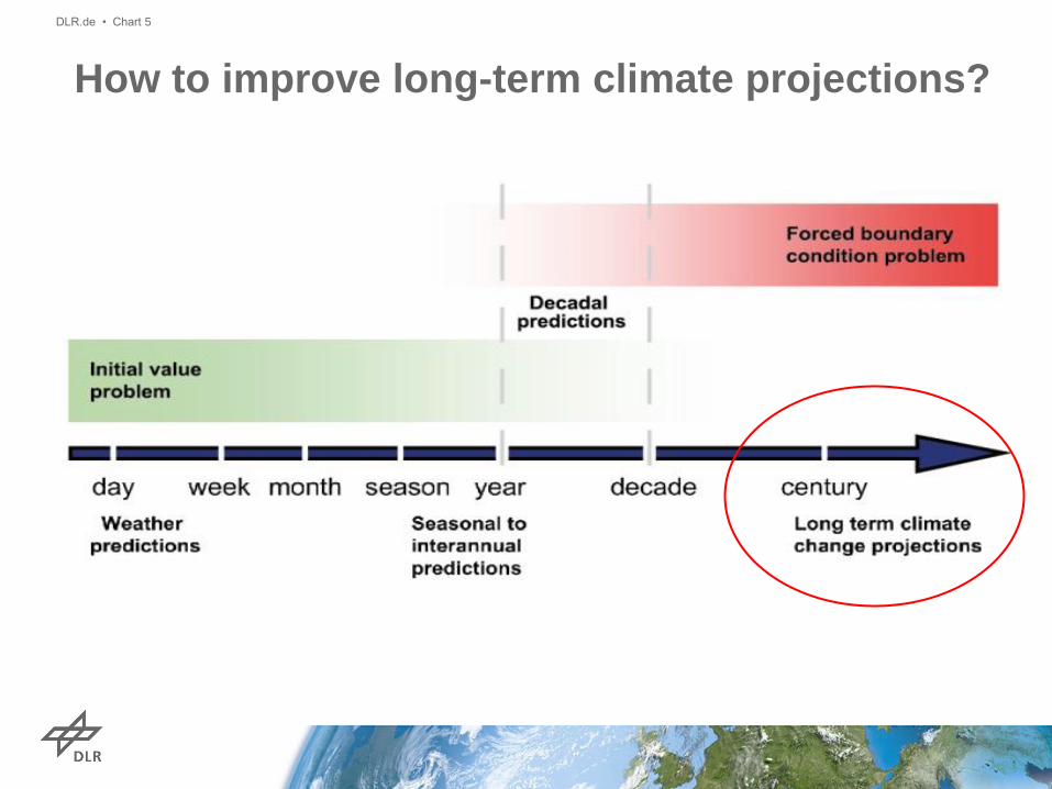
How to improve long-term climate projections?
DLR.de • Chart 5
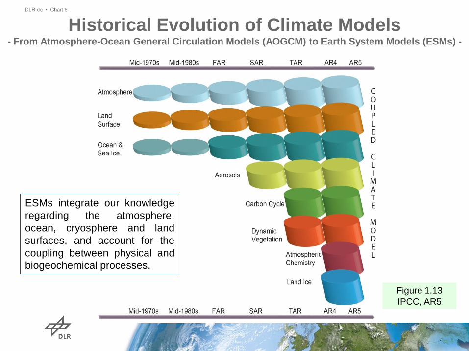
Historical Evolution of Climate Models - From Atmosphere-Ocean General Circulation Models (AOGCM) to Earth System Models (ESMs) -
DLR.de • Chart 6
Figure 1.13
IPCC, AR5
ESMs integrate our knowledge
regarding the atmosphere,
ocean, cryosphere and land
surfaces, and account for the
coupling between physical and
biogeochemical processes.
Coupled Model Intercomparison Project (CMIP) - Understanding past, present and future climate -
DLR.de • Chart 7
CMIP is a project of the World Climate Research Programme (WCRP)’s Working
Group of Coupled Modelling (WGCM).
Since 1995, CMIP has coordinated climate model experiments involving multiple
international modeling teams worldwide.
CMIP has led to a better understanding of past, present and future climate
change and variability in a multi-model framework.
CMIP defines common experiment protocols, forcings and output.
CMIP has developed in phases, with the simulations of the fifth phase, CMIP5,
now completed, and the planning of the sixth phase, i.e. CMIP6, well underway.
CMIP’s central goal is to advance scientific understanding of the Earth system.
CMIP model simulations have also been regularly assessed as part of the IPCC
Climate Assessments Reports and various national assessments.
The multi-model approach is now a standard technique to assess projections of specific
variables and to derive robust process understanding of the Earth’s climate system in
combination with observations.
1. Assessing the mechanisms responsible for model differences in poorly understood feedbacks
2. Estimating projection uncertainty
3. Determining why similarly forced models produce a range of responses.
DLR.de • Chart 8
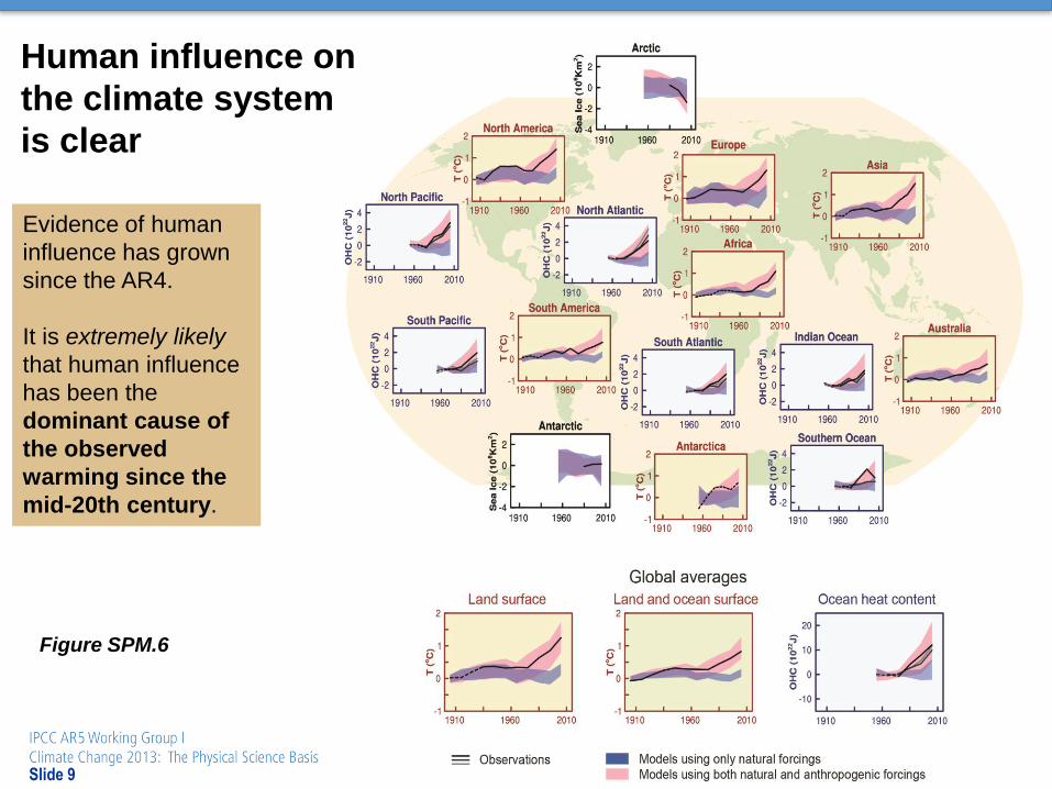
IPCC, Figure SPM.7a, 2014
IPCC FAQ 12.1, Figure 1
Why using an Ensemble of Model Simulation?
Evidence of human
influence has grown
since the AR4.
It is extremely likely
that human influence
has been the
dominant cause of
the observed
warming since the
mid-20th century.
Figure SPM.6
Slide 9
Human influence on
the climate system
is clear
2. How do we gain confidence in
climate model projections?
DLR.de • Chart 10
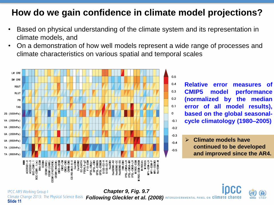
How do we gain confidence in climate model projections?
Chapter 9, Fig. 9.7
Following Gleckler et al. (2008)
Relative error measures of
CMIP5 model performance
(normalized by the median
error of all model results),
based on the global seasonal-
cycle climatology (1980–2005)
Slide 11
• Based on physical understanding of the climate system and its representation in
climate models, and
• On a demonstration of how well models represent a wide range of processes and
climate characteristics on various spatial and temporal scales
Climate models have
continued to be developed
and improved since the AR4.
A lot of progress has been made, but… DLR.de • Chart 12
Observations:
In many cases the lack or insufficient quality of long-term observations or observations for
process evaluation remains an impediment.
For many observational datasets formal error estimates are lacking.
Disagreement in observations complicate model evaluation (e.g. in cloud property trends), and
upper tropospheric / lower stratosphere (UTLS) temperature trends
Systematic Biases: e.g., Double Intertropical Convergence Zone (ITCZ), i.e. spurious ITCZ
in the SH associated with excessive tropical precipitation or the equatorward bias in the SH
atmospheric jet location
Precipitation
Equilibrium Climate Sensitivity Remains Uncertain
Equilibrium climate sensitivity (ECS):
• Response of the climate system to constant RF on multi-century time scales.
• Defined as the change in global mean surface temperature at equilibrium that is caused by
a doubling of the atmospheric CO2 concentration.
The model spread in ECS
ranges from 2.1°C to 4.7°C
and is very similar to the
assessment in AR4.
=> Due to uncertainties in climate feedbacks
3. CMIP6 Design
DLR.de • Chart 14
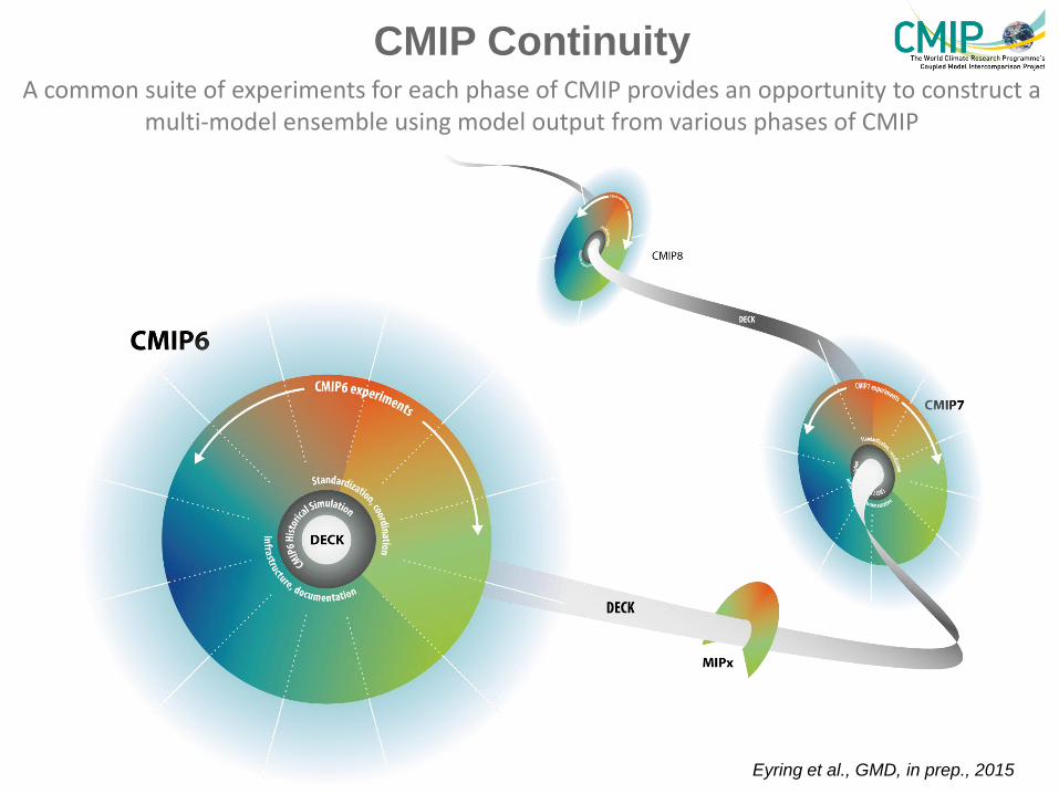
CMIP Continuity A common suite of experiments for each phase of CMIP provides an opportunity to construct a
multi-model ensemble using model output from various phases of CMIP
Eyring et al., GMD, in prep., 2015
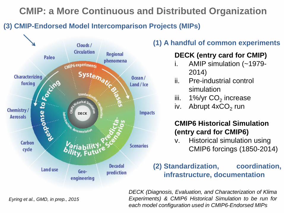
DECK (entry card for CMIP)
i. AMIP simulation (~1979-
2014)
ii. Pre-industrial control
simulation
iii. 1%/yr CO2 increase
iv. Abrupt 4xCO2 run
CMIP6 Historical Simulation
(entry card for CMIP6)
v. Historical simulation using
CMIP6 forcings (1850-2014)
CMIP: a More Continuous and Distributed Organization
(1) A handful of common experiments
(2) Standardization, coordination,
infrastructure, documentation
Eyring et al., GMD, in prep., 2015
DECK (Diagnosis, Evaluation, and Characterization of Klima
Experiments) & CMIP6 Historical Simulation to be run for
each model configuration used in CMIP6-Endorsed MIPs
(3) CMIP-Endorsed Model Intercomparison Projects (MIPs)
Models are increasing in complexity and resolution From AOGCMs to Earth System Models with biogeochemical cycles, from lowres to highres
(A) More routine evaluation of Earth system models with observations
DLR.de • Chart 18
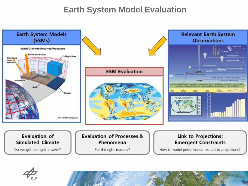
Earth System Model Evaluation
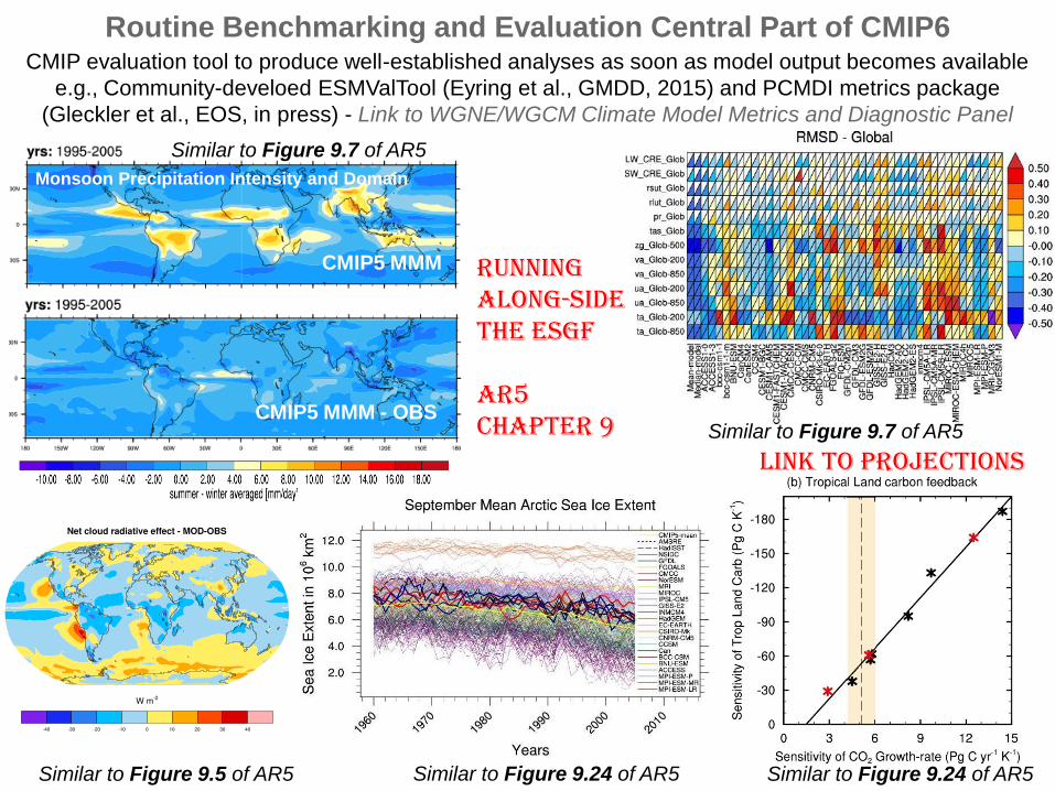
Routine Benchmarking and Evaluation Central Part of CMIP6 CMIP evaluation tool to produce well-established analyses as soon as model output becomes available
e.g., Community-develoed ESMValTool (Eyring et al., GMDD, 2015) and PCMDI metrics package
(Gleckler et al., EOS, in press) - Link to WGNE/WGCM Climate Model Metrics and Diagnostic Panel
Similar to Figure 9.7 of AR5
CMIP5 MMM
CMIP5 MMM - OBS
Monsoon Precipitation Intensity and Domain
Similar to Figure 9.7 of AR5
Running along-side the ESGF AR5 Chapter 9
Link to projections
Similar to Figure 9.24 of AR5 Similar to Figure 9.5 of AR5 Similar to Figure 9.24 of AR5
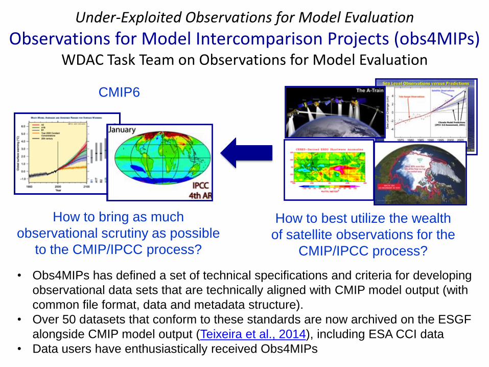
Under-Exploited Observations for Model Evaluation
Observations for Model Intercomparison Projects (obs4MIPs) WDAC Task Team on Observations for Model Evaluation
How to bring as much
observational scrutiny as possible
to the CMIP/IPCC process?
How to best utilize the wealth
of satellite observations for the
CMIP/IPCC process?
CMIP6
• Obs4MIPs has defined a set of technical specifications and criteria for developing
observational data sets that are technically aligned with CMIP model output (with
common file format, data and metadata structure).
• Over 50 datasets that conform to these standards are now archived on the ESGF
alongside CMIP model output (Teixeira et al., 2014), including ESA CCI data
• Data users have enthusiastically received Obs4MIPs
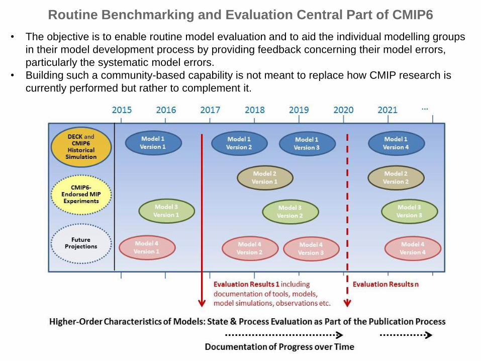
Routine Benchmarking and Evaluation Central Part of CMIP6
• The objective is to enable routine model evaluation and to aid the individual modelling groups
in their model development process by providing feedback concerning their model errors,
particularly the systematic model errors.
• Building such a community-based capability is not meant to replace how CMIP research is
currently performed but rather to complement it.
4. Opportunities for CMIP6
(B) Better consideration of internal variability and more
process-oriented evaluation
DLR.de • Chart 23
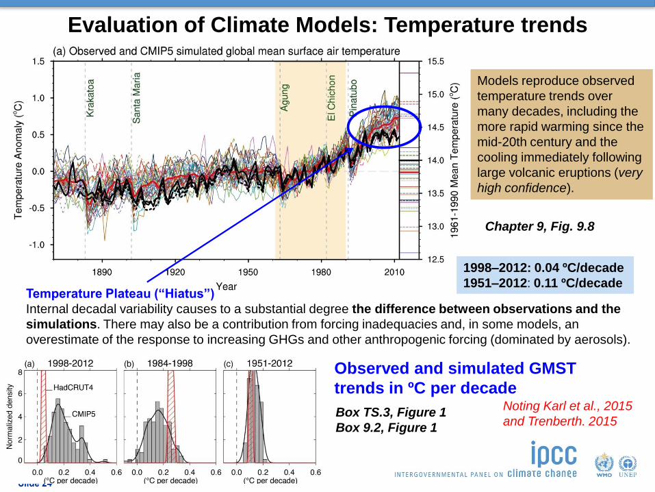
Evaluation of Climate Models: Temperature trends
Chapter 9, Fig. 9.8
Models reproduce observed
temperature trends over
many decades, including the
more rapid warming since the
mid-20th century and the
cooling immediately following
large volcanic eruptions (very
high confidence).
Slide 24
Temperature Plateau (“Hiatus”)
Internal decadal variability causes to a substantial degree the difference between observations and the
simulations. There may also be a contribution from forcing inadequacies and, in some models, an
overestimate of the response to increasing GHGs and other anthropogenic forcing (dominated by aerosols).
1998–2012: 0.04 ºC/decade
1951–2012: 0.11 ºC/decade
Box TS.3, Figure 1
Box 9.2, Figure 1
Observed and simulated GMST
trends in ºC per decade Noting Karl et al., 2015
and Trenberth. 2015
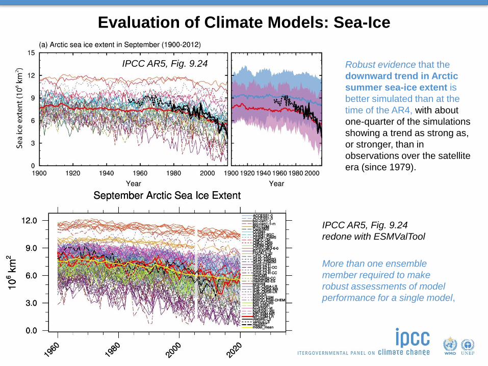
Evaluation of Climate Models: Sea-Ice
Robust evidence that the
downward trend in Arctic
summer sea-ice extent is
better simulated than at the
time of the AR4, with about
one-quarter of the simulations
showing a trend as strong as,
or stronger, than in
observations over the satellite
era (since 1979).
Slide 25
IPCC AR5, Fig. 9.24
More than one ensemble
member required to make
robust assessments of model
performance for a single model,
IPCC AR5, Fig. 9.24
redone with ESMValTool
Aim: to discover at what resolution climate processes are robustly simulated across multi-model ensemble
Example map of climate process and model
resolution required
CMIP6-Endorsed Model Intercomparison Project HighResMIP Co-chairs: Rein Haarsma & Malcolm Roberts
4. Opportunities for CMIP6
(C) Emergent constraints: Use of observations to constrain a simulated
future Earth system feedback
DLR.de • Chart 27
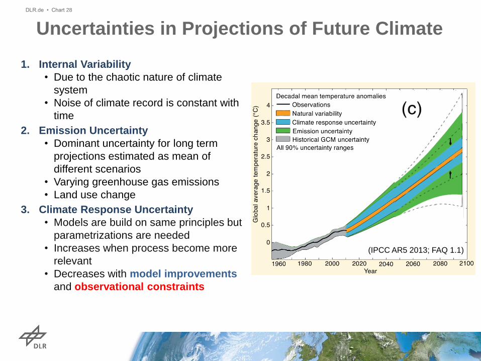
1. Internal Variability
• Due to the chaotic nature of climate
system
• Noise of climate record is constant with
time
2. Emission Uncertainty
• Dominant uncertainty for long term
projections estimated as mean of
different scenarios
• Varying greenhouse gas emissions
• Land use change
3. Climate Response Uncertainty
• Models are build on same principles but
parametrizations are needed
• Increases when process become more
relevant
• Decreases with model improvements
and observational constraints
Uncertainties in Projections of Future Climate
DLR.de • Chart 28
(IPCC AR5 2013; FAQ 1.1)
Constraint quantity of interest
Observational Constraint
O
bse
rved
ran
ge
Emergent Constraints (ECs) DLR.de • Chart 29
• ECs are a relationship across an ensemble of models, between some aspect of Earth
system sensitivity and an observable trend or variation in the current climate
Emergent because it emerges from the ensemble of ESMs.
Constraint because it enables an observation to constrain the estimate of the Earth System
sensitivity in the real world.
• The goal is to find a observable physical explanation to constrain the unobservable Earth
system sensitivity
Probability Density
Quantity of interest: sensitivity or future projection → Not observable
Observable variation (e.g. interannual or seasonal variability) or trend
Large intermodel variations in the strength of snow albedo feedback (SAF) in climate change in the NH in April are nearly perfectly correlated with comparably large intermodel variations in feedback strength in the context of the seasonal cycle.
Hall and Qu, GRL, 2006
Feedback strength in the real seasonal cycle can be observed and compared to models.
These mostly fall outside the range of the observed estimate, suggesting many models have an unrealistic snow albedo feedback in the seasonal cycle context.
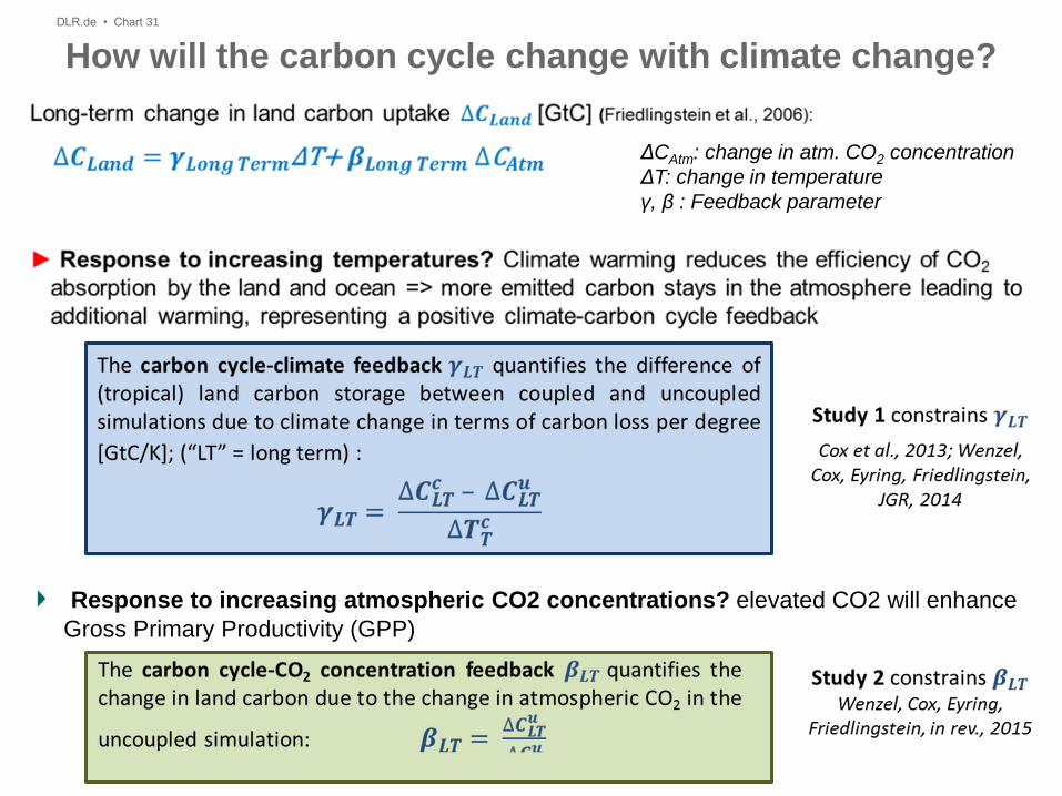
How will the carbon cycle change with climate change?
DLR.de • Chart 31
ΔCAtm: change in atm. CO2 concentration
ΔT: change in temperature
γ, β : Feedback parameter
Response to increasing atmospheric CO2 concentrations? elevated CO2 will enhance
Gross Primary Productivity (GPP)
DLR.de • Chart 32
Wenzel et al., JGR, 2014
Climate change is uncoupled to the carbon cycle Climate change is coupled to the carbon cycle
Ne
t ca
rbo
n flu
x f
rom
la
nd
to
atm
osp
he
re
(Ne
t B
iom
e P
rod
uctivity -
NB
P)
• Atmospheric CO2 concentration increased
over the last 50 years by approx. 100
ppmv
• Increasing atmospheric CO2 concentration
(black) mainly due to anthropogenic CO2
emissions
• Seasonal variability (red) due to seasonal
carbon cycle
Summer: more photosynthesis =>
atmospheric CO2 decreases stored in
terrestrial ecosystem
Winter: CO2 release by
decomposition of soil organic matter
Atmospheric CO2 Measurements
DLR.de • Chart 33
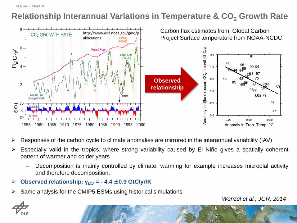
Relationship Interannual Variations in Temperature & CO2 Growth Rate
DLR.de • Chart 34
2
4
6
8
Global(NOAA)
Cape Grim(CSIRO)
0
30
Fossil Fuel
Pinatubo
1955 1960 1965 1970 1975 1980 1985 1990 1995 2000
-30
CO2 GROWTH RATE
El Nino
La Nina
Mauna Loa(Scripps/NOAA)
(R J Francey, pers. Com)
http://www.esrl.noaa.gov/gmd/publications
Responses of the carbon cycle to climate anomalies are mirrored in the interannual variability (IAV)
Especially valid in the tropics, where strong variability caused by El Niño gives a spatially coherent
pattern of warmer and colder years
Decomposition is mainly controlled by climate, warming for example increases microbial activity
and therefore decomposition.
Observed relationship: γIAV = - 4.4 ±0.9 GtC/yr/K
Same analysis for the CMIP5 ESMs using historical simulations
Observed
relationship
Carbon flux estimates from: Global Carbon
Project Surface temperature from NOAA-NCDC
Wenzel et al., JGR, 2014
DLR.de • Chart 35
CMIP5
Ob
serv
atio
nal
Co
nst
rain
t
Wenzel et al., JGR, 2014
PDF of pure
CMIP5 ensemble
Conditional PDF
where OBS are known
Applying MDER to future Austral Jet Stream Positions
DLR.de • Chart 36
• Multiple Diagnostic Ensemble Regression
(MDER, Karpechko et al., 2013)
Uses process-oriented present day diagnostics
to constrain future austral jet stream positions
• Equatorward bias of the CMIP5 models austral jet
positions with a spread of 10°
• MDER is targeted to constrain near-term (2015-
2034) projections of the austral jet position, and
selects the historical jet position as the most
important of 20 diagnostics.
• The method essentially recognizes the equatorward
bias in the past jet position, and provides a bias
correction of about 1.5° southward to future
projections. Wenzel et al., J. Clim., in press
Weighting Model Projections: Arctic Sea-Ice Process-based constraints can be used to reduce the spread of model projections
Figure 12.31
First year during which the September
Arctic sea ice extent falls below a certain
threshold is highly correlated with the
September sea ice extent and annual mean
sea ice volume averaged over the past.
First year during which the September
Arctic sea ice extent falls below a certain
threshold are correlated with the past trend
in September Arctic sea ice extent and the
amplitude of the mean seasonal cycle of
sea ice extent.
Suggests a faster rate of summer Arctic sea ice
decline than the multi-model mean
A model is retained if, for each diagnostic,
either this interval overlaps a ±20% interval
around the observed/reanalysed value of the
diagnostic or at least one ensemble member
from that model gives a value for the
diagnostic that falls within ±20% of the
observational/reanalysed data.
.
Fir
st y
ear
du
rin
g w
hic
h t
he
Sep
tem
ber
Arc
tic
sea
ice
exte
nt
falls
bel
ow
106
km2
Sep
tem
ber
Arc
tic
sea
ice
exte
nt
(106
km2 )
Slide 37
Massonnet et al., 2012
Other Examples on Selected Feedbacks and ECS
• The extratropical surface cryosphere feedback was constrained by Crook & Forster
(2014) using variations in the seasonal cycle of the cryosphere. Models were found to
largely underestimate this feedback (0.4 – 1.2 W m-2 K-1 compared to 3.1 ± 1.3 W m-2 K-1)
under warming despite their comparable seasonal sensitivity to observations.
• Gordon et al. (2013) related the water vapor feedback to observed variability (2002-2009)
Demonstrated the physical explanation of the relation between short and long-term
forced changes in models under warming.
However, relative weak relation combined with large uncertainties in the observations.
Suggested an observational record of 25 years or longer could significantly improve the
demonstrated observational constraint.
• Tian (2015) shows that show that the double-
ITCZ bias and ECS in 44 GCMs from CMIP 3/5
are negatively correlated Southern ITCZ index: model climatological annual
mean precip bias over southeastern Pacific
Low sensitivity models having problems in
representing its southern branch.
ECS might be in the higher end of its range
(~4.0°C) and most CMIP3/5 models might have
underestimated ECS.
Constraining Equilibrium Climate Sensitivity
DLR.de • Chart 39
Sherwood et al., 2014
• Spread in ECS arises largely from low clouds
• Relates ECS to the strength of mixing in the
lower troposphere over warm tropical oceans
(lower-tropospheric mixing index LTMI)
• Higher-sensititivity models simulate certain
cloud-relevant phenomena better.
• However, the metric suffers from large
uncertainties in the observed estimates.
Fasullo et al., 2015
• No final conclusions can be made yet, but
the results of EC studies generally suggest
an underestimation of ECS by models due to
cryospheric and cloud feedbacks.
radiosondes and reanalyses
Summary
While progress has been made in ESM evaluation over the last decades, there are
important opportunities and challenges for CMIP6, with simulations starting in 2016
DLR.de • Chart 40
In many cases the lack or insufficient quality of long-term observations or
observations for process evaluation remains an impediment, but improvements can
be made by fully exploiting existing observations and by taking into account
observational uncertainty.
Make the evaluation of CMIP models with well-established diagnostics and
performance metrics more routine (by developing and applying diagnostic tools
such as the ESMValTool) to leave more time for innovative research.
Part of the difference between model results and observations can be attributed to
unforced variability, originating from the nonlinear nature of the variable climate
system. An accurate assessment of model performance therefore has to take into
account internal climate variability in addition to observational uncertainty.
Summary Emergent Constraints
DLR.de • Chart 41
While evaluation of the evolving climate state and processes can be used to build
confidence in model fidelity, this does not guarantee the correct response to
changed forcing in the future.
Emergent constraint analysis refers to the use of observations to constrain a
simulated future Earth system feedback offers the potential to reduce uncertainty
in climate projections.
Studies have been published that focus both on constraining ECS more generally,
but also on constraining individual key feedbacks at a process level.
ECs studies can help guiding model development onto processes crucial to the
magnitude and spread of future Earth system change. This can also be used to
prioritize future observations activities.
A necessary property of emergent constraints is a physical basis for the relation.
There are many open questions and issues, but emergent constraints remain a
promising approach that should be fully exploited in CMIP analysis.