JOURNAL OF GEOPHYSICAL RESEARCH, VOL. 98, NO. C7, PAGES 12,417-12,429, JULY 15, 1993

East Antarctic Sea Ice:

Albedo, Thickness Distribution, and Snow Cover

IAN A• • IqON

Antarctic Cooperative Research Centre and Australian Antarctic Division, Hobart, Tasmania

RICH• E. BRANDT 1 AND STEPHEN G. WARREN

Geophysics Program, University of Washington, Seattle

Characteristics of springtime sea ice off East Antarctica were investigated during a cmise of the Australian National Antarctic Research Expedition in October through December 1988. The fractional coverage of the ocean surface, the ice thickness, and the snow cover thickness for each of several ice types were estimated hourly for the region near the ship. These observations were carried out continuously during the 4 weeks the ship was in the ice. Thin and young ice types were prevalent throughout the region, and the observations show a systematic increase in the total area-weighted pack ice thickness (including open water area) from only 0.2 m within 50 km of the ice edge to 0.45 m close to the coast. Ice thickness averaged over the ice-covered region only is also relatively thin, ranging from 0.35 m near the ice edge to 0.65 m in the interior. These values are probably typical of average winter thickness for the area. The average snow cover thickness on the ice increased from 0.05 m near the ice edge to 0.15 m in the interior. Average ice concentration increased from less than 6/10 near the ice edge to 8/10 in the interior. The ship-observed concentrations were in good agreement with concentrations derived from passive microwave satellite imagery except in some regions of high concentration. In these regions the satellite-derived concentrations were consistently lower than those estimated from the ship, possibly because of the inability of the satellite sensors to discriminate the appreciable percentage of very thin ice observe d within the total area. Spectral albedo was measured for nilas, young grey ice, grey- white ice, snow-covered ice, and open water at wavelengths from 420 to 1000 nm. Allwave albedo was computed by using the spectral measurements together with estimates of near-infrared albedo and modeled spectral solar flux. Area-averaged albedos for the East Antarctic sea ice zone in spring were derived from representative allwave albedos together with the hourly observations of ice types. These area-averaged surface albedos increased from about 0.35 at the ice edge to about 0.5 at 350 km from the edge, remaining at 0.5 to the coast of Antarctica. The low average albedo is in part due to the large fraction of open water within the pack, but extensive fractions of almost snow-free thin ice also play an important role.

INTRODUCI•ON

Antarctic sea ice consists mostly of young or first-year ice because most of the ice melts during the first summer after it forms. The difference in sea ice area in the Antarctic Ocean from its maximum extent in September or October to its minimum extent in February is about 16 million km 2 [Zwally et al., 1983], nearly as much area as South America covers so its influence on climate is potentially considerable.

Sea ice cover strongly influences the local climate and also affects global climate [Allison, 1982]. It modifies the air-sea energy exchange by increasing the surface albedo and insulating the relatively warm ocean from the atmosphere in winter. Within the seasonal sea ice zone, however, the sea ice is not a uniform slab but rather a highly mobile mix of ice of different thicknesses as well as open water in leads and polynyas. Even a small fraction of snow-free thin ice and open water within the pack can greatly modify the total energy transfer between ocean and atmosphere by turbulence and radiation [Maykut, 1978; Worby and Allison, 1991]. Recent studies of ice characteristics and drift [Allison, 1989; Jacka et al., 1987] have shown that although the total East Antarctic ice concentration in spring is 8/10 to 10/10 (80-

1Now at Burr and Burton Seminary, Manchester, Vermont.

Copyright 1993 by the American Geophysical Union.

Paper number 93JC00648. 0148-0227/93/93JC-00648505.00

100% ice cover), much of the ice is young and thin (typically• less than 0.3 m) and is constantly changing with ice drift, and the area-averaged ice thickness within the sea ice zone may be less than 0.4 m.

In this paper we present further observations of ice characteristics within the late spring East Antarctic sea ice zone (which confirm the results of the earlier studies) and measurements of the radiative properties of the ice. From these we derive preliminary estimates of the frequency distribution of ice and snow thickness and of the area-averaged surface albedo.

Sea ice first forms from randomly oriented frazil crystals, which in calm ocean conditions aggregate into a uniform thin sheet called nilas. (Definitions and photographs of the various forms of sea ice and other terminology of the sea-ice zone are given by the World Meteorological Organization (WMO) [1970] and Steffen [1986].) The nilas may then grow downward by freezing of water onto its base. The upper frazil layer normally has a much larger bubble concentration than does the lower "congelation" layer, whose crystals are more uniformly oriented. If there is significant wave action, the frazil agglomerates into nearly circular discs, initially tens of centimeters in diameter, instead of forming nilas. These "pancakes" adhere to each other and raft, growing into aggregates a few meters across and eventually forming a continuous, consolidated ice cover up to tens of centimeters thick [Lange et al., 19 89].

Snowfall is frequent in the Antarctic Ocean because of the passage of synoptic storms, so the young sea ice normally acquires a covering of snow within a few days after it forms.

12,417

12,418 ALLISON ET AL.: ALBEDO AND THICKNESS OF ANTARCTIC SEA ICE

In our observations sea ice thicker than 15 cm always had a snow cover. After snow has fallen on the ice, the albedo is determined by the snow thickness and grain sizes rather than by the air bubbles in the ice below. The snow albedo decreases slightly with age (as the grain size increases), but Antarctic sea ice rarely develops the melt ponds that are characteristic of Arctic sea ice in the ablation season and that

modify the regional albedo [Andreas and Ackley, 1982]. Solar radiation, essentially all at wavelengths between 300

and 3000 nm, is a major source of energy for the ice pack during the melting season. The shortwave (which we will call "allwave" to contrast with "spectral") albedo, or, of the variety of ice types we observed spanned the range 0.11-0.89 and thus is a major controlling variable for the energy budget of sea ice. The most important variable determining sea ice albedo is the presence or absence of snow cover. For young sea ice on which snow has not yet fallen, sunlight is reflected at the upper surface and is also scattered by air bubbles and brine pockets in the interior of the ice. The albedo is relatively low and is controlled by the size and number of air bubbles (and brine pockets) and the ice thickness. The albedo of darker varieties of snow-free ice can increase significantly as the solar elevation decreases. These dependences were discussed for lake ice by Mullen and Warren [1988] and for sea ice by Grenfell [1979, 1991]. The processes controlling air bubble and brine pocket numbers and sizes and their effect on albedo were modeled by Grenfell [ 1983].

A snow cover of only a few centimeters is quite effective in hiding the underlying ice, so that the albedo of the sea ice becomes essentially that of snow. The albedo of snow is determined principally by the snow grain size (albedo decreasing as the grains grow, especially rapidly in wet snow), but it is also sensitive to snow thickness for snow layers thinner than a few centimeters. Of secondary importance for snow albedo are the solar zenith angle (albedo increasing as the sun lowers) and cloud cover (total albedo increasing as cloud thickness increases) [Wiscombe and Warren, 1980; Warren, 1982].

A comprehensive set of spectral albedo measurements was made for snow-covered and melting Arctic sea ice by Grenfell and Perovich [1984]. The typical ice types in the Antarctic, however, are quite different: multiyear ice, bare melting sea ice, and melt puddles are rare but large areas are covered by thin new ice which forms in leads continually opened by the generally unconstrained northward divergence of the pack. Optical measurements on thin ice were made in the laboratory by Perovich and Grenfell [1981] and in the Arctic in a freezing lead by Perovich [1990]. In the Antarctic, allwave albedos of late-springtime sea ice were measured from aircraft off East Antarctica by Babarykin et al. [1965] and over the Ross Sea by Predoehl and Spano [1965] and Spano [1965]. Albedo was measured from a ship in the Atlantic sector of the Antarctic by Andreas and Makshtas [1985]. These various measurements are compared with our results below.

A focus of our experiment was to measure how Antarctic sea ice albedo varies with wavelength. Such spectral measurements are needed in order to design a remote-sensing strategy for sea ice by means of narrow-channel radiometers on polar-orbiting satellites. Because the transmittance of clouds varies with wavelength, spectral surface albedo is also needed to estimate the allwave albedo under different

thicknesses of cloud. We measured the spectral albedos of several types of new ice, young ice, and snow-covered first- year ice. The spectral albedo of thin wintertime Antarctic sea ice has previously been measured by Schlosser [1988], and that of melting sea ice in McMurdo Sound (apparently not snow covered) has been measured by Kuhn and Siogas [1978]. The latter results agreed with Grenfell and Maykut's [1977]

spectral albedo of melting first-year ice in the Arctic from 400 to 1000 nm.

FIELD PROGRAM

The field program, part of the Australian National Antarctic Research Expeditions (ANARE), was carried out aboard MV Icebird during the first spring season voyage in October through December 1988. Ice characteristics were recorded hourly throughout the cruise to continue the observational analysis begun by Allison [1989], and 22 ship-based and helicopter-based measurements of spectral albedo were made for a variety of sea ice types in the wavelength region 420- 1000nm. By combining the results of the albedo measurements with the sea ice observations, average allwave albedos are presented as a function of distance from the ice edge for springtime conditions in the Indian Ocean sector of East Antarctica. The responses of advanced very high resolution radiometer (AVHRR) channels 1 and 2 on National Oceanic and Atmospheric Administration (NOAA) satellites were also calculated for the observed sea ice types.

Icebird travelled the route Hobart-Casey-Davis-Mawson- Hobart. The purpose of the voyage was to exchange personnel and equipment at three Australian stations on the coast of East Antarctica (Casey, Davis, and Mawson). Icebird entered the sea ice pack on 28 October and exited on 23 November (Figure 1). Generally, spring conditions were encountered, with nighttime growth of nilas common in open water, along with a general breakup of the ice pack with time, resulting in southward retreat of the ice edge. The location of the ice edge, based on visible and microwave satellite images, was mapped weekly during the voyage by the U.S.Navy-NOAA Joint Ice Center (JIC) and every 10 days by the USSR Antarctic Meteorological Center Molodezhnaya Ice Analysis Program. These ice edge and ice concentration maps were in reasonable agreement with each other. Both were available by facsimile aboard Icebird. A composite ice edge for the duration of the cruise, derived from the JIC charts, is shown in Figure 1.

SEA ICE AND SNOW CHARACTERISrHCS

Hourly observations of ice characteristics were made visually within a range of 0.5 nautical miles of the ship's bridge during the time the vessel was in the ice. At each observation, up to three different ice types according to the WMO 1970 ice nomenclature (new ice (frazil, shuga, grease), nilas, pancake ice, young grey ice, young grey-white ice, etc.) were discriminated. For each of these ice types, estimates were made of concentration, ice thickness, floe size, floe topography, snow cover type, and snow thickness. Total concentration, category of open water (lead, pool, polynya, etc.), and surface meteorological conditions were also observed. Simultaneous visual observations were frequently made from the forward lower deck as close as possible to ice floes turned on their sides by the passage of the ship to better gauge the accuracy of ice thickness and snow depth estimates. The accuracy of individual thickness observations is probably about 20%, but the large sample of observations can be expected to provide a good statistical description of the late- spring pack ice characteristics, particularly at the thin end of the thickness distribution, where changes are most important for both radiant and turbulent heat transfer [e.g., Worby and Allison, 1991 ].

To avoid bias toward the thick-ice categories in areas of heavy ice, when the ship's speed was less than 6 knots, only observations taken more than 6 nautical miles apart were included in the analysis. Ice statistics were compiled with respect to the distance south of the outer ice edge shown on

ALLISON ET AL.: ALBEDO AND TI IICKNESS OF ANTARCTIC SEA ICE 12,419

56

58

60

62

• 64

66

68

70

..... observations from aircraft

C) regions of short helicopter flights

28 OCT

19 NOV Li.

58 62

AVIS ........

ß ' MIRNY ......

66 70 74 78 82 86 90 94 98 102 106 110 114 118

LONGITUDE (øE)

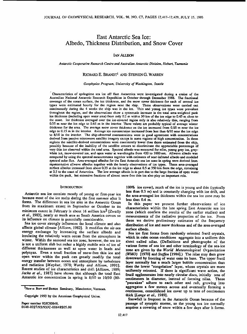
Fig. 1. Route of MV Icebird through the sea ice pack, October and November 1988. Also shown are the number of hourly ice observations made in each 2 ø x 4 ø latitude-longitude grid box and a composite ice edge showing the northerly limit of ice at each longitude at the time the ship was on that longitude. The ice edge was derived from the weekly U.S.Navy-NOAA JIC ice charts.

the JIC ice charts, as longitudinal variation of the ice edge over the cruise track made analysis by latitude inappropriate. Another expected bias, difficult to quantify, was a result of the primary objective of the voyage to resupply the Australian stations. Since the ship was seeking the route of least resistance, the ice observations might be biased toward thinner ice types. However, aircraft observations of the pack during nine helicopter flights of distances up to 90 km from the ship and during two fixed-wing aircraft flights over the southeastern sector of Prydz Bay and between Davis and 67.5øS, 75øE (see Figure 1) confirmed that total concentration, floe size, and percentage of young (dark) ice categories over the general region were similar to those observed from the ship.

A total of 426 hourly observations were made. However, only one observation for each 6-nautical-mile segment of the route was used in the analysis, giving a total of 301 observations. The number of observations for each 2 ø latitude

4 ø . x longitude grid box is shown in Figure 1 Figure 2 and Figures 4 through 8 show scattergrams of some of the observed ice characteristics correlated with distance from the

ice edge. Although the pack conditions were highly variable over even short distances, as evidenced by the large spread of observations, there was a statistically significant trend in most variables with distance from the ice edge.

Ship-Observed and Satellite-Derived Ice Concentrations

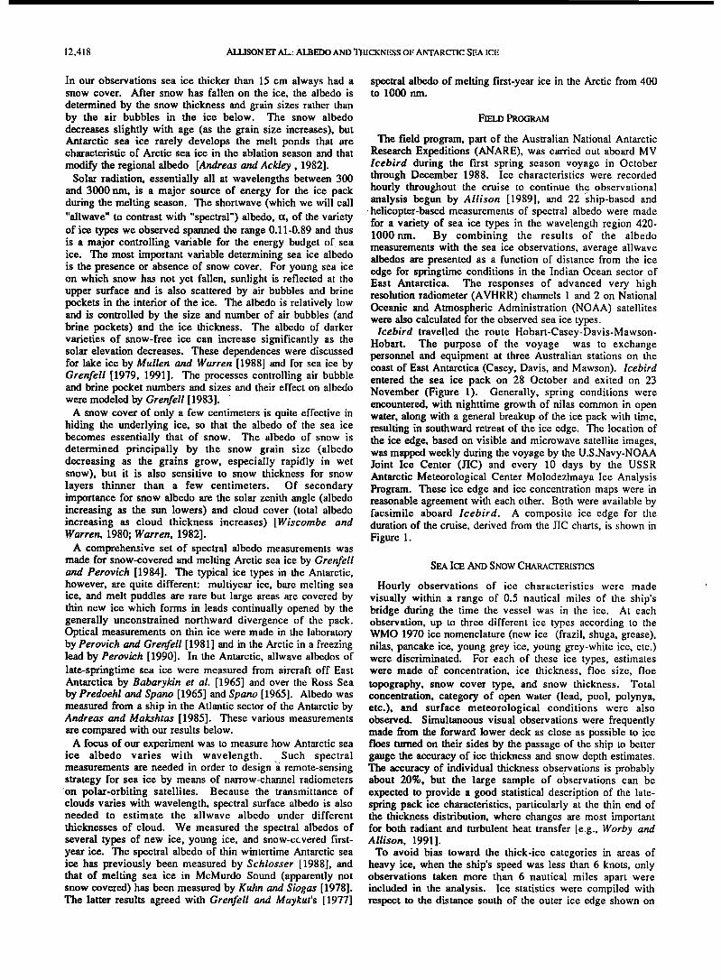
In general the total ice concentration (or ice fraction) increased as the distance from the ice edge increased, as shown in Figure 2. Extreme variation of the total concentration near the ice edge was observed, with areas of open water in the form of large leads and polynyas interspersed with bands of ice that reached 10/10 concentration. Open water was much less common farther south in the ice pack until the flaw lead was reached just north of the shorefast ice edge.

These observations of ice concentration provide an opportunity to verify the National Air and Space

Administration (NASA) Team sea ice algorithm used to derive concentration from the multichannel SSM/I satellite microwave data [Cavalieri et al., 1984]. (CD-ROM copies of the daily microwave-derived ice concentrations are available for the period since July 1987 on a 25 x 25 km grid from the National Snow and Ice Data Center, Boulder, Colo.) We identified in which grid square the shipboard observations were made and averaged all concentration observations for each pixel. Because the ship track covered only a relatively small area within a grid square, the observed concentrations are highly variable between squares. Hence the data were smoothed with a centered running average 5 pixels in length.

c- 7

10-øeø eel ß

el ß • ß eel el eel ß ee • ß e•ee •e ß e• ee ß

I-•e ß ee ß e ee ß ee ß ß ß ß ß

eeee ..... • ß ee ß ß ß

ß i ß i ß i ß i ß i , i , i

0 100 200 300 400 500 600 700

distance from ice edge (km)

Fig. 2. Total ice concentration (ice cover fraction) versus distance from the ice edge. Only observations at least 6 nautical miles apart are included. Solid bars are zonal mean concentrations.

12,420 ALLISON ET AL.: ALBEDO AND THICKNESS OF ANTARCTIC SEA ICE

This length was chosen because it produced a pixel-to-pixel variation in the ship-derived concentrations similar to that in the SSM/I concentration estimates while still retaining the similarity between major features in the two data sets.

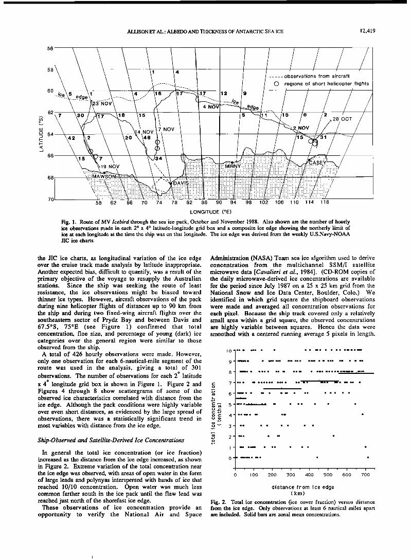
The differences between the ship estimate and that from the NASA Team algorithm are shown against the smoothed ship concentrations in Figure 3. The two estimates are in reasonable agreement between 3/10 and 8/10 concentration, but at high concentrations the ship estimates are consistently higher than the satellite estimates, whereas at low concentrations the satellite estimates are higher. Very similar results were obtained by Steffen [1991] in a comparison of microwave-derived concentrations in the Northwater (between Ellesmere Island and Greenland) with concentrations derived from Landsat imagery.

Over the total track the mean difference between the two

estimates was only 0.33/10 (3.3% fractional cover) with a standard deviation of 1.42/10. The highest microwave ice concentration in pixels along the track was 8.7, while the ship-based estimates gave averages as high as 9.5. It was in these regions of high ice concentration that reconnaissance helicopter flights to find possible ship routes were made and areas larger than an entire pixel were observed. The heaviest ice was encountered during the approach to Casey when Icebird was unable to reach the station. During several extensive helicopter reconnaissances, no areas of concentration of less than 9/10 were observed, although the NASA Team algorithm estimated concentrations between 5/10 and 8/10. In many of the high-concentration ice areas we observed a considerable fraction of new, "black" nilas within the total ice cover, and the difference between the ship-based and satellite estimates of total concentration at high concentration may be a result of the inability of the passive microwave instrument to distinguish very thin ice from open water [Cavalieri et al., 1984].

Ice Thickness and Snow Cover

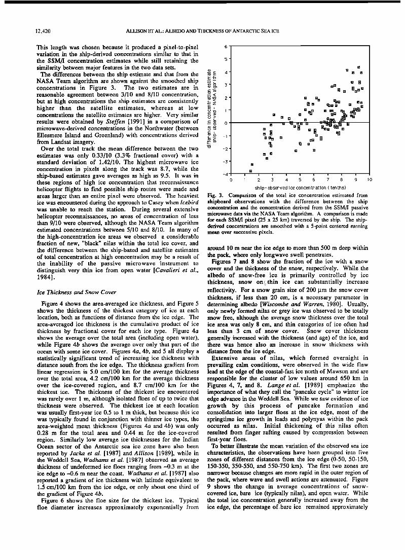
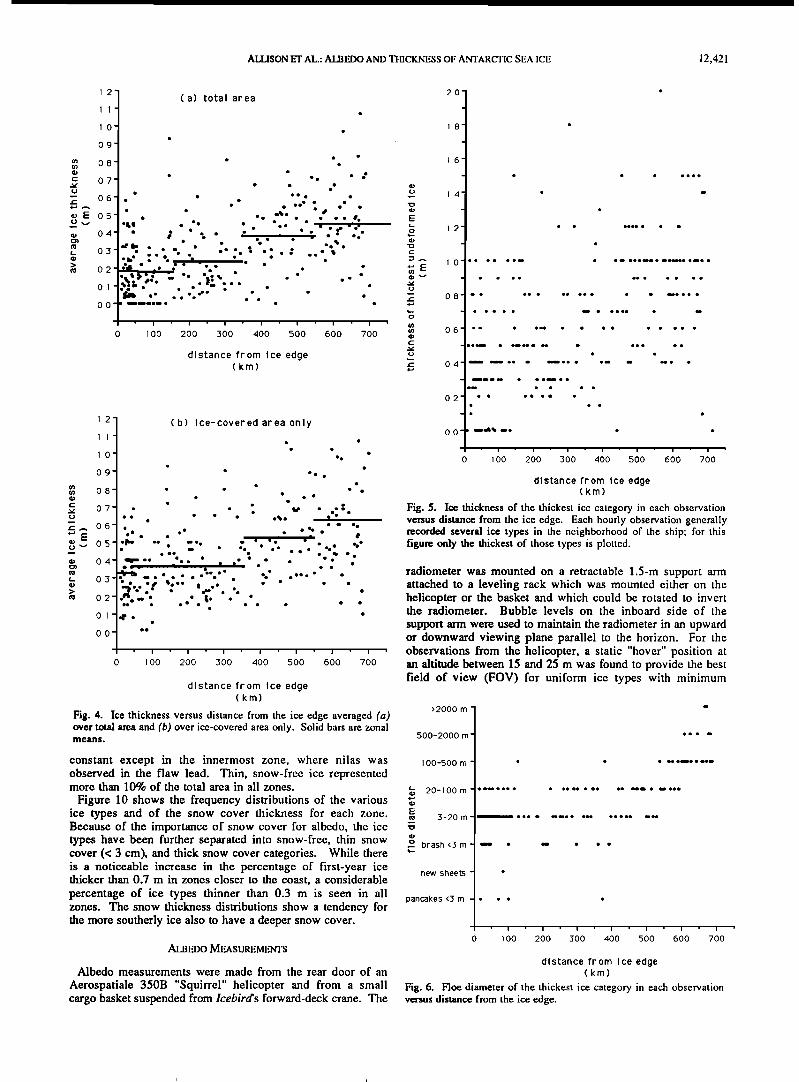
Figure 4 shows the area-averaged ice thickness, and Figtire 5 shows the thickness of the thickest category of ice at each location, both as functions of distance from the ice edge. The area-averaged ice thickness is the cumulative product of ice thickness by fractional cover for each ice type. Figure 4a shows the average over the total area (including open water), while Figure 4b shows the average over only that part of the ocean with some ice cover. Figures 4a, 4b, and 5 all display a statistically significant trend of increasing ice thickness with distance south from the ice edge. The thickness gradient from linear regression is 5.0 cm/100 km for the average thickness over the total area, 4.2 cm/100 km for the average thickness over the ice-covered region, and 8.7 cm/100 km for the thickest ice. The thickness of the thickest ice encountered

was rarely over 1 m, although isolated floes of up to twice that thickness were observed. The thickest ice at each location

was usually first-year ice 0.5 to 1 m thick, but because this ice was typically found in conjunction with thinner ice types, the area-weighted mean thickness (Figures 4a and 4b) was only 0.28 m for the total area and 0.44 m for the ice-covered

region. Similarly low average ice thicknesses for the Indian Ocean sector of the Antarctic sea ice zone have also been

reported by Jacka et al. [1987] and Allison [1989], while in the Weddell Sea, Wadhams et al. [1987] observed an average thickness of undeformed ice floes ranging from --0.3 m at the ice edge to --.0.6 m near the coast. Wadhams et al. [1987] also reported a gradient of ice thickness with latitude equivalent to 1.5 cm/100 km from the ice edge, or only about one third of the gradient of Figure 4b.

Figure 6 shows the floe size for the thickest ice. Typical floe diameter increases approximately exponentially from

5 '

4'

3 '

2'

t

o

-1

-2

-3

-4

o

[]

[] []

[] []

i i i i i i i i i

1 2 3 4 $ 6 7 8 9 10

ship- observed ice concentration (tenths)

Fig. 3. Comparison of the total ice concentration estimated from shipboard observations with the difference between the ship concentration and the concentration derived from the SSM/I passive microwave data via the NASA Team algorithm. A comparison is made for each SSM/I pixel (25 x 25 km) traversed by the ship. The ship- derived concentrations are smoothed with a 5-point centered running mean over successive pixels.

around 10 m near the ice edge to more than 500 m deep within the pack, where only longwave swell penetrates.

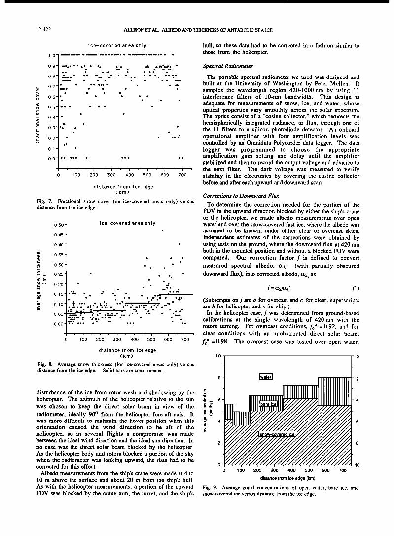
Figures 7 and 8 show the fraction of the ice with a snow cover and the thickness of the snow, respectively. While the albedo of snow-free ice is primarily controlled by ice thickness, snow on':f. thin ice can substantially increase reflectivity. For a snow grain size of 200 gm the snow cover thickness, if less than 20 cm, is a necessary parameter in determining albedo [Wiscombe and Warren, 1980]. Usually, only newly formed nilas or grey ice was observed to be totally snow free, although the average snow thickness over the total ice area was only 8 cm, and thin categories of ice often had less than 3 cm of snow cover. Snow cover thickness

generally increased with the thickness (and age) of the ice, and there was hence also an increase in snow thickness with

distance from the ice edge. Extensive areas of nilas, which formed overnight in

prevailing calm conditions, were observed in the wide flaw lead at the edge of the coastal-fast ice north of Mawson and are responsible for the cluster of low values around 650 km in Figures 4, 7, and 8. Lange et al. [1989] emphasize the importance of what they call the "pancake cycle" to winter ice edge advance in the Weddell Sea. While we saw evidence of ice growth by this process of pancake formation and consolidation into larger floes at the ice edge, most of the springtime ice growth in leads and polynyas within the pack occurred as nilas. Initial thickening of this nilas often resulted from finger rafting caused by compression between first-year floes.

To better illustrate the mean variation of the observed sea ice

characteristics, the observations have been grouped into five zones of different distances from the ice edge (0-50, 50-150, 150-350, 350-550, and 550-750 km). The first two zones are narrower because changes are more rapid in the outer region of the pack, where wave and swell actions are attenuated. Figure 9 shows the change in average concentrations of snow- covered ice, bare ice (typically nilas), and open water. While the total ice concentration generally increased away from the ice edge, the percentage of Jbare ice remained approximately

ALLISON ET AL.: ALBEDO AND TIIICKNESS OF ANTARCrIC SEA ICE 12,421

1'21 (a) total area 2o- 1.1 ß '

1.0 ß 18'

09 ø

08 0.7 06 . ø . ß oo•, ß ø .. ._ 1 4-

' . ' .. -'-. ;..,. •,• ß ß ee ß ß ß •-• o.• - ; ß • . :- . .:'j.• .-.. •o ,2- ß . :' ß

ß :.--.. .--...-.: ..., . .- : ,o- 02

y: o•-

oo 0 100 200 300 400 500 600 700

distance from ice edge (km)

12'

1 1-

10'

09-

08-

07

06

05

04

03

02'

01'

00'

(b) ice-covered area only

ß ß

ß

ß©

ß ß

ß

ß

ß ß

ß ß ß ß ß

ee • ß ß ee e#i• ee e• e e

ß ß ei

ß ß

II•II ee ß ß ee , ß ,

:.;.:'; '-" . .' e•I•e ee el ß eIe ß el ee ß eeee •e ß

ß

ß

ee

ee e ß ß

ß ß ß ß ß

ß

ß e ß ß e•e ß ,

ß • ß e ß ee ß

ß ß , ß • ß ß e ß ß ß eee ß ß e e ß ß eee

ß ß ß ß ß ee ß ß ß ß ß ß ß ß ß ß ß ß

ß

ß e eeee ß ß ß ß ß ß

ß

ß

ß ß

' i ß i ß i ß i ß i ß i ß i

0 100 200 300 400 500 600 700

distance from ice edge (km)

Fig. 4. Ice thickness versus distance from the ice edge averaged (a) over total area and (b) over ice-covered area only. Solid bars are zonal means.

constant except in the innermost zone, where nilas was observed in the flaw lead. Thin, snow-free ice represented more than 10% of the total area in all zones.

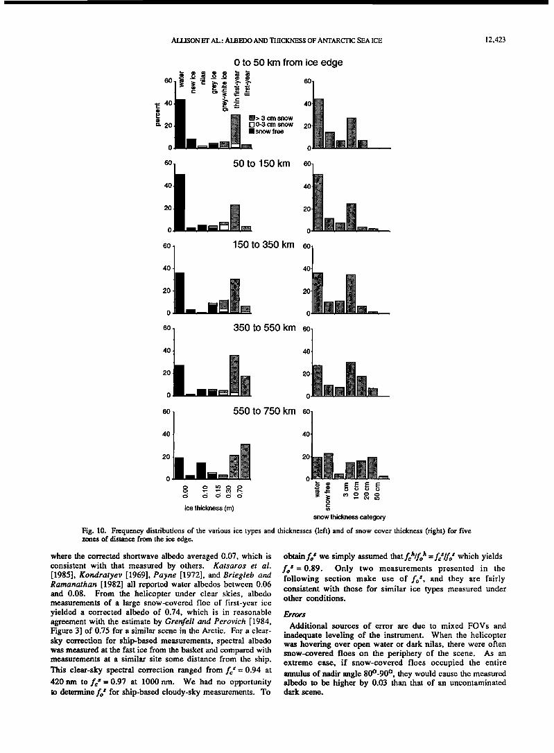
Figure 10 shows the frequency distributions of the various ice types and of the snow cover thickness for each zone. Because of the importance of snow cover for albedo, the ice types have been further separated into snow-free, thin snow cover (< 3 cm), and thick snow cover categories. While there is a noticeable increase in the percentage of first-year ice thicker than 0.7 m in zones closer to the coast, a considerable percentage of ice types thinner than 0.3 m is seen in all zones. The snow thickness distributions show a tendency for the more southerly ice also to have a deeper snow cover.

ALBEDO MEASUREMENTS

Albedo measurements were made from the rear door of an

Aerospatiale 350B "Squirrel" helicopter and from a small cargo basket suspended from Icebird's forward-deck crane. The

O2

00

ß

ß ß

ß

ß

ß ß

ß

ei

ß ee

I ß eeee

ß eeee

i

eeee ß ß •

ß i eeeei• ß eeeeee elß ß

ee ß ß ß ß ß

ß • ileee ß

ß ei

ß

- I Iee • eiiiee ß eei ee

II ii1# ß lille

ß

.

' i ' i ß i

0 100 200 300

ß i

400

ee

ß

elß ß

ß

ß

ß i ß i ß i .

500 600 700

distance from Ice edge (km)

Fig. 5. Ice thickness of the thickest ice category in each observation versus distance from the ice edge. Each hourly observation generally recorded several ice types in the neighborhood of the ship; for this figure only the thickest of those types is plotted.

radiometer was mounted on a retractable 1.5-m support arm attached to a leveling rack which was mounted either on the helicopter or the basket and which could be rotated to invert the radiometer. Bubble levels on the inboard side of the

support arm were used to maintain the radiometer in an upward or downward viewing plane parallel to the horizon. For the observations from the helicopter, a static "hover" position at an altitude between 15 and 25 m was found to provide the best field of view (FOV) for uniform ice types with minimum

>2000 m

500-2000 m

100-500 m

20-1 O0 rn

3-20 m

brash <3 rn

new sheets

pancakes <3 rn

.

-

- ß

- e•IIeee ß

-

i ß

ß

ß ß ß

ß i

o lOO

ß i ß i ß i ß i ß i ß i

200 300 400 500 600 700

distance from Ice edge (km)

Fig. 6. Floe diameter of the thickest ice category in each observation versus distance from the ice edge.

12,422 ALLISON ET AL.: ALB•O AND TIIICKNESS OF ANTARCTIC SEA ICE

1.0-

09'

08-

07'

0.6'

0.5'

0.4-

0.3-

02-

01'

00'

ice-covered area only

ileo ß ß ß; ß ß e

IiI

ß ß

©i ß

ß

ß

i

i© ß

ß

©© ß ß

ß

e © ß

o ß

ß © oo© ß ©© i ß ß ee

ß ß ß

o© ©o© ß

ß ß ß

ß ß ß

ß ß

©e

ß

ß ß e©

ß ß ß ß

ß ß ß ß ß

ß ß ß

ß

ß

ß

ß ©oo ø

ß i ß I ß i ß i . i ß i ß i

0 100 200 300 400 500 600 700

dlstance from lce edge (km)

Fig. 7. Fractional snow cover (on ice-covered areas only) versus distance from the ice edge.

0 50'

O. 45 '

0 40'

0 35'

0 30-

0 25'

0.20 '

015-

010-

0 05-

0.00

Ice-covered area only

ß ß ß

ß ß

ß ß ß

ß ß

ß ß

ß ß . ,.'

ß ee

ß eo ee ee ß

ß ß ß ß ß ß ß ee ß ß e •eI ß eo

• coo ß coo ß ß ' ? eo e ..:....:'. **v.. ' .•' b ß .*W ." eo ,, ß ß m ,, ß e• ß ß ß e e

e eoeoe ß eeoc ß ß • eeeo • ß eo ß

.•... ß '.'..- . ß ee ß ß el ß ee

ß i . i ß i ß i ß i , i ß i

0 1 O0 200 300 400 500 600 700

distance from ice edge (km)

Fig. 8. Average snow thickness (for ice-covered areas only) versus distance from the ice edge. Solid bars are zonal means.

disturbance of the ice from rotor wash and shadowing by the helicopter. The azimuth of the helicopter relative to the sun was chosen to keep the direct solar beam in view of the radiometer, ideally 90 ø from the helicopter fore-aft axis. It was more difficult to maintain the hover position when this orientation caused the wind direction to be aft of the

helicopter, so in several flights a compromise was made between the ideal wind direction and the ideal sun direction. In

no case was the direct solar beam blocked by the helicopter. As the helicopter body and rotors blocked a portion of the sky when the radiometer was looking upward, the data had to be corrected for this effect.

Albedo measurements from the ship's crane were made at 4 to 10 m above the surface and about 20 m from the ship's hull. As with the helicopter measurements, a portion of the upward FOV was blocked by the crane arm, the turret, and the ship's

hull, so these data had to be corrected in a fashion similar to those from the helicopter.

Spectral Radiometer

The portable spectral radiometer we used was designed and built at the University of Washington by Peter Mullen. It samples the wavelength region 420-1000 nm by using 11 interference filters of 10-nm bandwidth. This design is adequate for measurements of snow, ice, and water, whose optical properties vary smoothly across the solar spectrumß The optics consist of a "cosine collector," which redirects the hemispherically integrated radiance, or flux, through one of the 11 filters to a silicon photodiode detector. An onboard operational amplifier with four amplification levels was controlled by an Omnidata Polycorder data logger. The data logger was programmed to choose the appropriate amplification gain setting and delay until the amplifier stabilized and then to record the output voltage and advance to the next filter. The dark voltage was measured to verify stability in the electronics by covering the cosine collector before and after each upward and downward scan.

Corrections to Downward Flux

To determine the correction needed for the portion of the FOV in the upward direction blocked by either the ship's crane or the helicopter, we made albedo measurements over open water • and over the snow-covered fast ice, where the albedo was assumed to be known, under either clear or overcast skies. Independent estimates of the corrections were obtained by using tests on the ground, where the downward flux at 420 nm both in the mounted position and without a blocked FOV were compared. Our correction factor f is defined to convert measured spectral albedo, •x•.' (with partially obscured

downward flux), into corrected albedo, •x•., as

f= a•Ja•.' (1)

(Subscripts on f are o for overcast and c for clear; superscripts are h for helicopter and s for ship.)

In the helicopter case, f was determined from ground-based calibrations at the single wavelength of 420 nm with the rotors turning. For overcast conditions, fob= 0.92, and for clear conditions with an unobstructed direct solar beam,

fch= 0.98. The overcast case was tested over open water,

o

c•

10

100 200 300 400 500 600 7•

j o -2

4

8

10

•0

distance from ice edge (km)

Fig. 9. Average zonal concentrations of open water, bare ice, and snow-covered ice versus distance from the ice edge.

AIJJ$ON ET AL.: ALBEDO AND TIIICKNESS OF ANTARCTIC SEA ICE 12,423

0 to 50 km from ice edge

60.

40.

20.

60 50 to 150 km

40

20

0

60 150 to 350 km 60

40 401

20 .,.:•..,:.B ':•"=• O- -.m.__[ . .":'"'":-/-•. 60 350 to 550 km

40

20

60 550 to 750 km 60.

40 40'

21 [/.•./.i...•.':'"•'"'•. :':••. 2 I' :;...',••. •'"'::'"'•. ::.:...;•. •½:.....:j•...::........•. :.!........:••. :;-•. o o •oo • õ E 0 .,- ',% cO r-. '• ,_ o • • o• • •'• •oo•o

o

ice thickness (m) '- snow thickness category

Fig. 10. Frequency distributions of the various ice types and thicknesses (left) and of snow cover thickness (right) for five zones of distance from the ice edge.

where the corrected shortwave albedo averaged 0.07, which is consistent with that measured by others. Katsaros et al. [1985], Kondratyev [1969], Payne [1972], and Briegleb and Ramanathan [1982] all reported water albedos between 0.06 and 0.08. From the helicopter under clear skies, albedo measurements of a large snow-covered floe of first-year ice yielded a corrected albedo of 0.74, which is in reasonable agreement with the estimate by Grenfell and Perovich [ 1984, Figure 3] of 0.75 for a similar scene in the Arctic. For a clear- sky correction for ship-based measurements, spectral albedo was measured at the fast ice from the basket and compared with measurements at a similar site some distance from the ship. This clear-sky spectral correction ranged from fcS= 0.94 at 420 nm to fc s = 0.97 at 1000 nm. We had no opportunity to determine fo s for ship-based cloudy-sky measurements. To

_ $ $ obtain fo' we simply assumed that fch/fo n -fc/fo which yields fo' =0.89. Only two measurements presented in the following section make use of fo s, and they are fairly consistent with those for similar ice types measured under other conditions.

Errors

Additional sources of error are due to mixed FOVs and

inadequate leveling of the instrument. When the helicopter was hovering over open water or dark nilas, there were often snow-covered floes on the periphery of the scene. As an extreme case, if snow-covered floes occupied the entire annulus of nadir angle 80ø-90 ø, they would cause the measured albedo to be higher by 0.03 than that of an uncontaminated dark scene.

12,424 ALLISON ET AL.: ALBEDO AND THICKNESS OF ANTARCTIC SEA ICE

When a dark surface is viewed under an overcast sky, the downward looking measurement is contaminated with cloud if the inslxument is not level. However, an extreme tilt of 10 ø causes at most an albedo error of 0.01. Under clear sky, on the other hand, albedo errors due to tilt can be quite substantial for a different reason: the upward looking measurement has the wrong angle between the instrument and the direct beam. For example, at a solar zenith angle of 67 ø, a 2 ø tilt directly toward or away from the sun can cause an error of 10% of the albedo value. For tilt in any other direction the error is less, The error is smaller for high sun, so when the sky was clear, we tried to make measurements near local noon. For example, at a solar zenith angle of 45 ø, a tilt of 2 ø directly toward the sun would cause the downward flux to be overestimated by 3.6%. The upward flux is much less sub ect to tilt error because it is relatively diffuse. Under an overcast sky the tilt errors largely vanish and deviations from cosine response are also of much less consequence, so the most accurate albedos measured from the helicopter or the basket are those for uniform overcast.

The difference between the two scans for each ice type, shown in Figure 11 and discussed in the next section, suggest that our actual albedo errors due to tilt are a few percent. The errors are much smaller on the fast ice (riPpermost curve) because the instrument was suspended between tripods planted firmly in the snow and was leveled accurately. The fast-ice plot is the only one in Figure 11 that was not measured from helicopter or basket.

SPECTRAL AND ALLWAVE ALBEDOS OF SEA ICE

Spectral Albedo

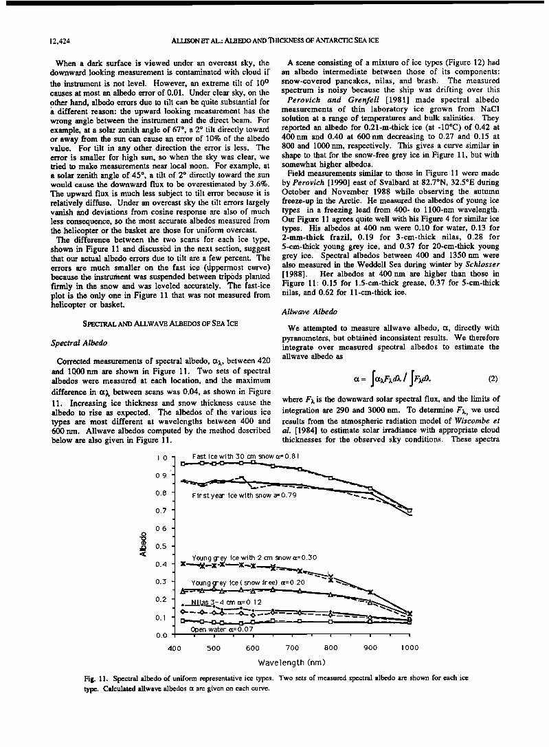
Corrected measurements of spectral albedo, ot•., between 420 and 1000 nm are shown in Figure 11. Two sets of spectral albedos were measured at each location, and the maximum

difference in ot•, between scans was 0.04, as shown in Figure 11. Increasing ice thickness and snow thickness cause the albedo to rise as expected. The albedos of the various ice types are most different at wavelengths between 400 and 600 nm. Allwave albedos computed by the method described below are also given in Figure 11.

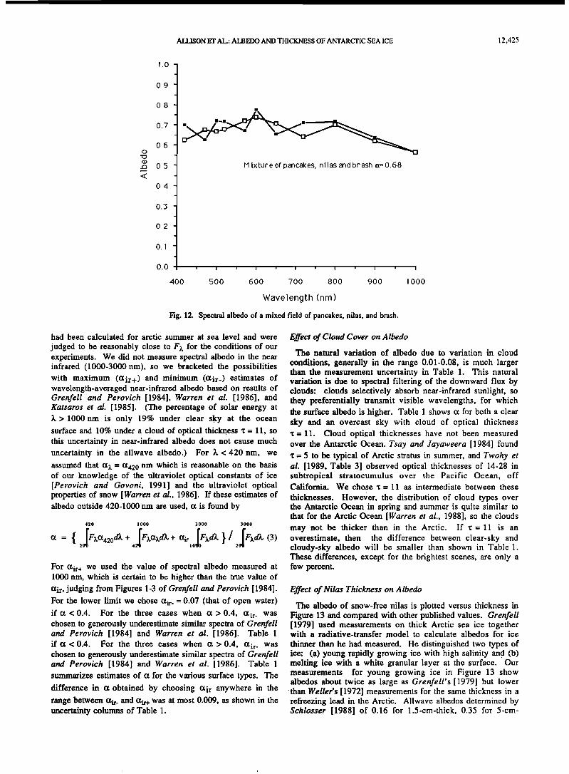
A scene consisting of a mixture of ice types (Figure 12) had an albedo intermediate between those of its components: snow-covered pancakes, nilas, and brash. The measured spectrum is noisy because the ship was drifting over this

Perovich and Grenfell [1981] made spectral albedo measurements of thin laboratory ice grown from NaC1 solution at a range of temperatures and bulk salinities. They reported an albedo for 0.21-m-thick ice (at -10øC) of 0.42 at 400nm and 0.40 at 600nm decreasing to 0.27 and 0.15 at 800 and 1000 nm, respectively. This gives a curve similar in shape to that for the snow-free grey ice in Figure 11, but with somewhat higher albedos.

Field measurements similar to those in Figure 11 were made by Perovich [1990] east of Svalbard at 82.7øN, 32.5øE during October and November 1988 while observing the autumn freeze-up in the Arctic. He measured the albedos of young ice types in a freezing lead from 400- to 1100-nm wavelength. Our Figure 11 agrees quite well with his Figure 4 for similar ice types. His albedos at 400 nm were 0.10 for water, 0.13 for 2-mm-thick frazil, 0.19 for 3-cm-thick nilas, 0.28 for 5-cm-thick young grey ice, and 0.37 for 20-cm-thick young grey ice. Spectral albedos between 400 and 1350 nm were also measured in the Weddell Sea during winter by Schlosser [1988]. Her albedos at 400 nm are higher than those in Figure 11:0.15 for 1.5-cm-thick grease, 0.37 for 5-cm-thick nilas, and 0.62 for 11-cm-thick ice.

Allwave Albedo

We attempted to measure allwave albedo, or, directly with pyranometers, but obtained inconsistent results. We therefore integrate over measured spectral albedos to estimate the allwave albedo as

(2) where F•. is the downward solar spectral flux, and the limits of integration are 290 and 3000 nm. To determine F•., we used results from the atmospheric radiation model of Wiscombe et al. [1984] to estimate solar irradiance with appropriate cloud thicknesses for the observed sky conditions. These spectra

1.0 - Fast ice with 30 cm snow a=0.81 ß

0.9

0.8 First year ice with snow a =0.79 ••.••••_ 0.7

0.6 o

• 0.5 i

Young grey ice with 2 cm snow a=0.30

0.3 Young grey ice ( snow free) a=0.20

0.2 , Nil•.s ,3,• 4 cm a=O. 1 2 - -o26: --o_ o'•-6--"=•---6.---

o, • • _• _ _ Open water a=0.07

400 500 600 700 800 900 •000

Wavelength (rim)

Fig. 11. S•ctral al•do of unifo• representative ice types. Two sets of measured spectral albedo am shown for each ice ty•. Calculated allwave albedos • am given on each cu•e.

ALLISON ET AL.: ALBEDO AND THICKNESS OF ANTARCTIC SEA ICE 12,425

1.0

0.9

0.8

0.7

0.6

0.5

0.4

0.3

0.2

0.1

0.0

Mixture of pancakes, nilas and brash •=0.68

400

I I I • I I I t I I I

500 600 700 800 900 1000

Wavelength (nm)

Fig. 12. Spectral albedo of a mixed field of pancakes, nilas, and brash.

had been calculated for arctic summer at sea level and were

judged to be reasonably close to FZ. for the conditions of our experiments. We did not measure spectral albedo in the near infrared (1000-3000 nm), so we bracketed the possibilities with maximum (t•ir+) and minimum (t•ir_) estimates of wavelength-averaged near-infrared albedo based on results of Grenfell and Perovich [1984], Warren et al. [1986], and Katsaros et al. [1985]. (The percentage of solar energy at )• > 1000nm is only 19% under clear sky at the ocean surface and 10% under a cloud of optical thickness 'c = 11, so this uncertainty in near-infrared albedo does not cause much uncertainty in the allwave albedo.) For )• < 420 nm, we assumed that t•. = 0;420 nm which is reasonable on the basis of our knowledge of the ultraviolet optical constants of ice [Perovich and Govoni, 1991] and the ultraviolet optical properties of snow [Warren et al., 1986]. If these estimates of albedo outside 420-1000 nm are used, t• is found by

420 1000 3000 3000

2 4 10 2

For t•ir + we used the value of spectral albedo measured at 1000 nm, which is certain to be higher than the true value of t•ir, judging from Figures 1-3 of Grenfell and Perovich [ 1984].

For the lower limit we chose O;ir.- 0.07 (that of open water)

if t• < 0.4. For the three cases when t• > 0.4, O;ir. was chosen to generously underestimate similar spectra of Grenfell and Perovich [1984] and Warren et al. [1986]. Table 1 if •t < 0.4. For the three cases when t• > 0.4, O;ir. was chosen to generously underestimate similar spectra of Grenfell and Perovich [1984] and Warren et al. [1986]. Table 1 summarizes estimates of tx for the various surface types. The

difference in t• obtained by choosing t•ir anywhere in the range between •r- and t•ir + was at most 0.009, as shown in the uncertainty columns of Table 1.

Effect of Cloud Cover on Albedo

The natural variation of albedo due to variation in cloud

conditions, generally in the range 0.01-0.08, is much larger than the measurement uncertainty in Table 1. This natural variation is due to spectral filtering of the downward flux by clouds: clouds selectively absorb near-infrared sunlight, so they preferentially transmit visible wavelengths, for which the surface albedo is higher. Table 1 shows tx for both a clear sky and an overcast sky with cloud of optical thickness x = 11. Cloud optical thicknesses have not been measured over the Antarctic Ocean. Tsay and Jayaweera [1984] found x = 5 to be typical of Arctic stratus in summer, and Twohy et al. [1989, Table 3] observed optical thicknesses of 14-28 in subtropical stratocumulus over the Pacific Ocean, off California. We chose x = 11 as intermediate between these

thicknesses. Howe•er, the distribution of cloud types over the Antarctic Ocean in spring and summer is quite similar to that for the Arctic Ocean [Warren et al., 1988], so the clouds

may not be thicker than in the Arctic. If 'c = 11 is an overestimate, then the difference between clear-sky and cloudy-sky albedo will be smaller than shown in Table 1. These differences, except for the brightest scenes, are only a few percent.

Effect of Nilas Thickness on Albedo

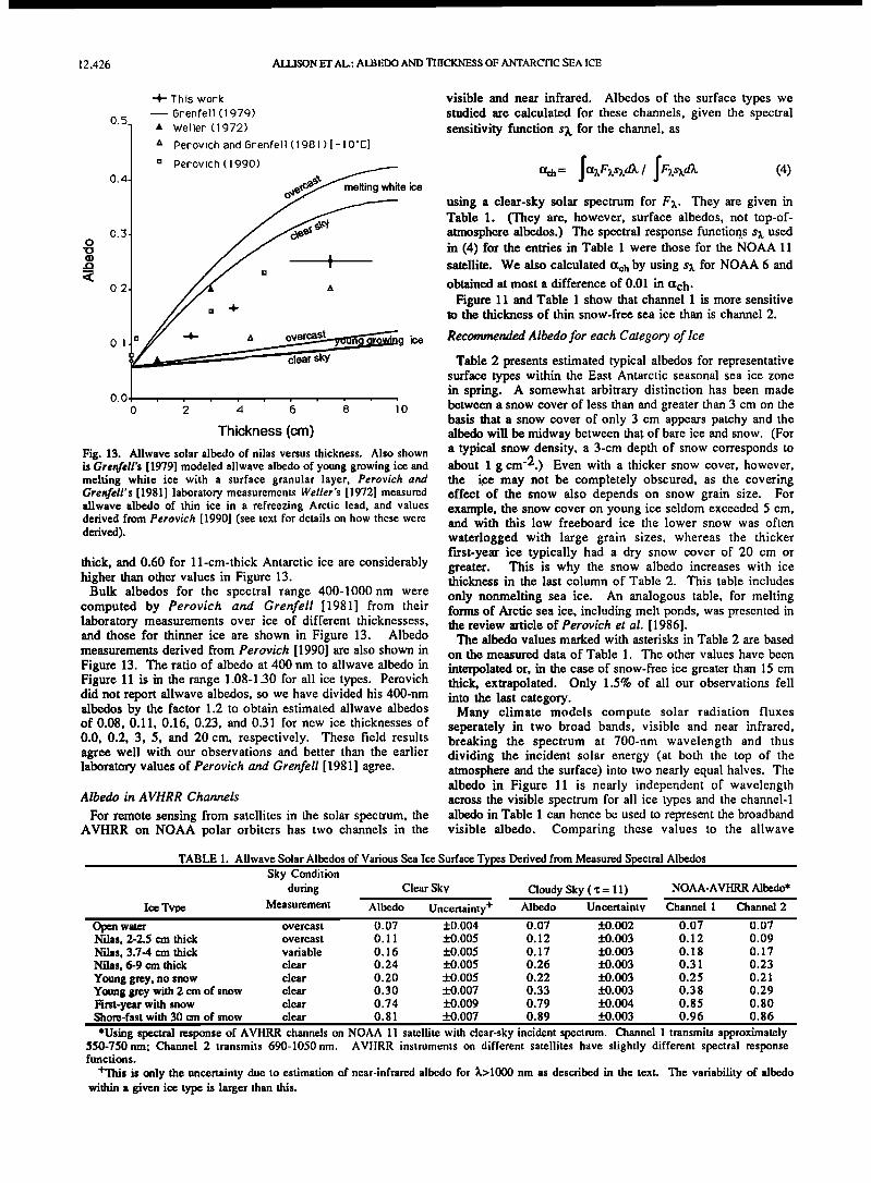
The albedo of snow-free nilas is plotted versus thickness in Figure 13 and compared with other published values. Grenfell [1979] used measurements on thick Arctic sea ice together with a radiative-transfer model to calculate albedos for ice

thinner than he had measured. He distinguished two types of ice: (a) young rapidly growing ice with high salinity and (b) melting ice with a white granular layer at the surface. Our measurements for young growing ice in Figure 13 show albedos about twice as large as Grenfell's [1979] but lower than Weller's [1972] measurements for the same thickness in a refreezing lead in the Arctic. Allwave albedos determined by Schlosser [1988] of 0.16 for 1.5-cm-thick, 0.35 for 5-cm-

12,426 ALLISON ET AL.: ALBEDO AND TI IICKNESS OF ANTARCFIC SEA ICE

0.5

0.4

-•- This work

• Grenfell (1979)

ß Weller (1972)

a Perovich and Grenfell (1981 ) [- 100c]

a Perovich (1990)

melting white ice

o 0.3

0.2

0.1

sky

ice

0.0

0 2 4 6 8 10

Thickness (cm)

Fig. 13. Allwave solar albedo of nilas versus thickness, Also shown is Grenfell's [1979] modeled allwave albedo of young growing ice and melting white ice with a surface granular layer, Perovich and Grenfell's [1981] laboratory measurements Weller's [1972] measured allwave albedo of thin ice in a refreezing Arctic lead, and values derived from Perovich [1990] (see text for details on how these were derived).

thick, and 0.60 for 11-cm-thick Antarctic ice are considerably higher than other values in Figure 13.

Bulk albedos for the spectral range 400-1000 nm were computed by Perovich and Grenfell [1981] from their laboratory measurements over ice of different thicknessess, and those for thinner ice are shown in Figure 13. Albedo measurements derived from Perovich [1990] are also shown in Figure 13. The ratio of albedo at 400 nm to allwave albedo in Figure 11 is in the range 1.08-1.30 for all ice types. Perovich did not report allwave albedos, so we have divided his 400-nm albedos by the factor 1.2 to obtain estimated allwave albedos of 0.08, 0.11, 0.16, 0.23, and 0.31 for new ice thicknesses of 0.0, 0.2, 3, 5, and 20 cm, respectively. These field results agree well with our observations and better than the earlier laboratory values of Perovich and Grenfell [1981] agree.

Albedo in A VHRR Channels

For remote sensing from satellites in the solar spectrum, the AVHRR on NOAA polar orbiters has two channels in the

visible and near infrared. Albedos of the surface types we studied are calculated for these channels, given the spectral sensitivity function s)• for the channel, as

•:h= $•zFzszd•/$Fzszd• (4) using a clear-sky solar spectrum for Fz. They are given in Table 1. (They are, however, surface albedos, not top-of- atmosphere albedos.) The spectral response functions s z used in (4) for the entries in Table 1 were those for the NOAA 11 satellite. We also calculated c•ch by using sz for NOAA 6 and

obtained at most a difference of 0.01 in C•ch. Figure 11 and Table 1 show that channel 1 is more sensitive

to the thickness of thin snow-free sea ice than is channel 2.

Recommended Albedo for each Category of Ice

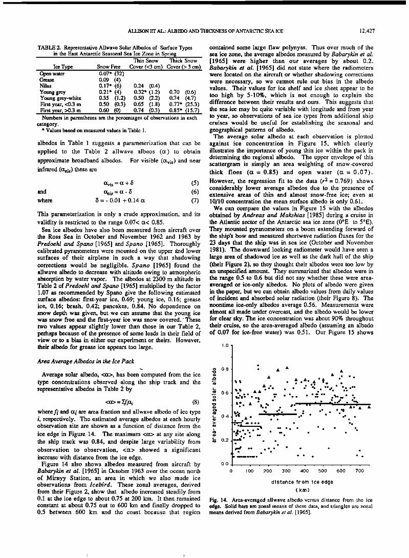
Table 2 presents estimated typical albedos for representative surface types within the East Antarctic seasonal sea ice zone in spring. A somewhat arbitrary distinction has been made between a snow cover of less than and greater than 3 cm on the basis that a snow cover of only 3 cm appears patchy and the albedo will be midway between that of bare ice and snow. (For a typical snow density, a 3-cm depth of snow corresponds to about 1 g cm-2.) Even with a thicker snow cover, however, the ice may not be completely obscured, as the covering effect of the snow also depends on snow grain size. For example, the snow cover on young ice seldom exceeded 5 cm, and with this low freeboard ice the lower snow was often

waterlogged with large grain sizes, whereas the thicker first-year ice typically had a dry snow cover of 20 cm or greater. This is why the snow albedo increases with ice thickness in the last column of Table 2. This table includes

only nonmelting sea ice. An analogous table, for melting forms of Arctic sea ice, including melt ponds, was presented in the review article of Perovich et al. [1986].

The albedo values marked with asterisks in Table 2 are based on the measured data of Table 1. The other values have been

interpolated or, in the case of snow-free ice greater than 15 cm thick, extrapolated. Only 1.5% of all our observations fell into the last category.

Many climate models compute solar radiation fluxes seperately in two broad bands, visible and near infrared, breaking the spectrum at 700-nm wavelength and thus dividing the incident solar energy (at both the top of the atmosphere and the surface) into two nearly equal halves. The albedo in Figure 11 is nearly independent of wavelength across the visible spectrum for all ice types and the channel-1 albedo in Table 1 can hence be used to represent the broadband visible albedo. Comparing these values to the allwave

TABLE 1. Allwave Solar Albedos O f Various Sea Ice Surface Types Derived from Measured Spectral Albedos Sky Condition

during Clear Sky Cloudy Sky ( x = 11) Ice Tvl•e Measurement Albedo Uncertainty + Albedo Uncertainty Channel 1 Channel 2

Open water overcast 0.'07 +0.004 0.07 ' +0.002 0.07 0.07 Nilas, 2-2.5 cm thick overcast 0.11 +0.005 0.12 +0.003 0.12 0.09 Nilas, 3.7-4 cm thick variable 0.16 +0.005 0.17 +0.003 0.18 0.17 Nilas, 6-9 cm thick clear 0.24 +0.005 0.26 +0.003 0.31 0.23 Young grey, no snow clear 0.20 +0.005 0.22 +0.003 0.25 0.21 Young grey with 2 cm of snow clear 0.30 +0.007 0.33 +0.003 0.38 0.29 First-year with snow clear 0.74 +0.009 0.79 +0.004 0.85 0.80 Shore-fast with 30 crn of snow clear 0.81 +0.007 0.89 +0.003 0.96 0.86

NOAA-AVHRR Albedo*

*Using spectral response of AVIIRR channels on NOAA 11 satellite with clear-sky incident spectrum. Channel 1 transmits approximately 550-750nm; Channel 2 transmits 690-1050nm. AVHRR instruments on different satellites have slightly different spectral response functions.

+This is only the uncertainty due to estimation of near-infrared albedo for •.>1000 nm as described in the text. The variability of albedo within a given ice type is larger than this.

ALLISON ET AL.: ALBEDO AND TI IICKNESS OF ANTARCTIC SEA ICE 12,427

TABLE 2. Representative Allwave Solar Albedos of Surface Types in the East Antarctic Seasonal Sea Ice Zone in Sprint3

Thin Snow 'lhick Snow

Ice Type Snow Free Open water 0.07* (32) Grease 0.09 (4) Nilas 0.17' (6) Young grey 0.21' (4) Young grey-white 0.35 (1.2) First year, <0.3 m 0.50 (0.3) First year, >0.3 m 0.60 (0)

Cover (<3.cm) Cover(> 3 C TM)

0.24 (0.4) 0.32* (1.2) 0.70 (0.6) 0.50 (2.2) 0.74 (4.7) 0.65 (1.8) 0.77* (25.3) 0.74 (0.3) 0.85* (15.7)

Numbers in parentheses are the percentages of observations in each category.

* Values based on measured values in Table 1.

albedos in Table 1 suggests a parameterization that can be applied to the Table 2 allwave albeos (ix) to obtain

approximate broadband albedos. For visible (avis) and near infrared (otnir) these are

and

where

avis = tx + $ (5) Otn•r = tz - •5 (6)

= - 0.01 + 0.14 (x (7)

This parameterization is only a crude approximation, and its validity is restricted to the range 0.07< ix< 0.85.

Sea ice albedos have also been measured from aircraft over

the Ross Sea in October and November 1962 and 1963 by Predoehl and Spano [1965] and Spano [1965]. Thoroughly calibrated pyranometers were mounted on the upper and lower surfaces of their airplane in such a way that shadowing corrections would be negligible. Spano [1965] found the allwave albedo to decrease with altitude owing to atmospheric absorption by water vapor. The albedos at 2300 m altitude in Table 2 of Predoehl and Spano [1965] multiplied by the factor 1.07 as recommended by Spano give the following estimated surface albedos: first-year ice, 0.69; young ice, 0.16; grease ice, 0.16; brash, 0.42; pancakes, 0.84. No dependence on snow depth was given, but we can assume that the young ice was snow free and the first-year ice was snow covered. These two values appear slightly lower than those in our Table 2, perhaps because of the presence of some leads in their field of view or to a bias in either our experiment or theirs. However, their albedo for grease ice appears too large.

Area Average Albedos in the Ice Pack

Average solar albedo, <or>, has been computed from the ice type concentrations observed along the ship track and the representative albedos in Table 2 by

<a> = 7.f,,m (8)

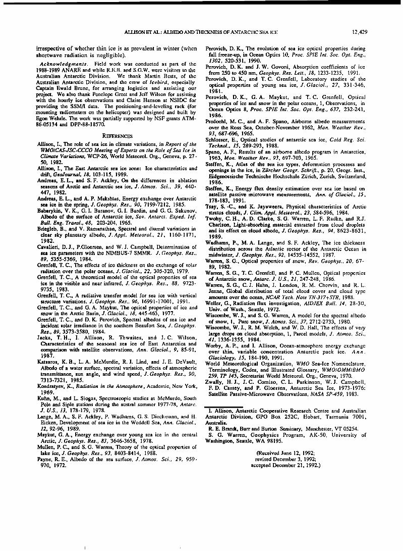
whereft' and ot i are area fraction and allwave albedo of ice type i, respectively. The estimated average albedos at each hourly observation site are shown as a function of distance from the

ice edge in Figure 14. The maximum <ix> at any site along the ship track was 0.84, and despite large variability from observation to observation, <or> showed a significant increase with distance from the ice edge.

Figure 14 also shows albedos measured from aircraft by Babarykin et al. [1965] in October 1963 over the ocean north of Mirnyy Station, an area in which we also made ice observations from Icebird. These zonal averages, derived from their Figure 2, show that albedo increased steadily from 0.1 at the ice edge to about 0.75 at 200 kin. It then remained constant at about 0.75 out to 600 km and finally dropped to 0.5 between 600 km and the coast because that region

contained some large flaw polynyas. Thus over much of the sea ice zone, the average albedos measured by Babarykin et al. [1965] were higher than our averages by about 0.2. Babarykin et al. [1965] did not state where the radiometers were located on the aircraft or whether shadowing corrections were necessary, so we cannot rule out bias in the albedo values. Their values for ice shelf and ice sheet appear to be too high by 5-10%, which is not enough to explain the difference between their results and ours. This suggests that the sea ice may be quite variable with longitude and from year to year, so observations of sea ice types from additional ship cruises would be useful for establishing the seasonal and geographical patterns of albedo.

The average solar albedo at each observation is plotted against ice concentration in Figure 15, which clearly illustrates the importance of young thin ice within the pack in determining the regional albedo. The upper envelope of this scattergram is simply an area weighting of snow-covered thick floes (or = 0.85) and open water (ix = 0.07).

However, the regression fit to the data (r2= 0.769) shows considerably lower average albedos due to the presence of extensive areas of thin and almost snow-free ice; even at 10/10 concentration the mean surface albedo is only 0.61.

We can compare the values in Figure 15 with the albedos obtained by Andreas and Makshtas [1985] during a cruise in the Atlantic sector of the Antarctic sea ice zone (0øE to 5øE). They mounted pyranometers on a boom extending forward of the ship's bow and measured shortwave radiation fluxes for the 23 days that the ship was in sea ice (October and November 1981). The downward looking radiometer would have seen a large area of shadowed ice as well as the dark hull of the ship (their Figure 2), so they thought their albedos were too low by an unspecified amount. They summarized that albedos were in the range 0.5 to 0.6 but did not say whether these were area- averaged or ice-only albedos. No plots of albedo were given in the paper, but we can obtain albedo values from daily values of incident and absorbed solar radiation (their Figure 8). The noontime ice-only albedos average 0.56. Measurements were almost all made under overcast, and the albedo would be lower for clear sky. The ice concentration was about 90% throughout their cruise, so the area-averaged albedo (assuming an albedo of 0.07 for ice-free water) was 0.51. Our Figure 15 shows

1.0

0.8

0.2

0.0

ß ß ß

ß ß ß ß ß

0 100 200 300 400 500 600 700

distance from ice edge (km)

Fig. 14. Area-averaged allwave albedo versus distance from the ice edge. Solid bars are zonal means of these data, and triangles are zonal means derived from Babarykin et al. [1965].

12,428 ALLISON ET AL.: ALBEDO AND TIIICKNESS OF ANq'ARCTIC SEA ICE

lO

0.8

ß

0.6

• o4

0.2

0.0

ice concentration

(tenths)

Fig. 15. Area-averaged allwave albedo versus ice concentration. The regression fit to the data points is also shown.

average albedos of 0.57 and 0.62 for ice concentrations of 90 and 100%, respectively, that is, higher than those of Andreas and Makshtas by 0.06. This could be due to their omission of a correction for shadowing by the ship rather than to a regional difference in ice types.

DISCUSSION AND CONCLUSIONS

Figure 16 summarizes the average total area-weighted ice thickness and surface albedo and the average snow thickness on the ice-covered areas. These are derived from the

observations of Figures 4, 8, and 14 for each zone of distance from the ice edge. The total area-weighted ice thickness increased from less than 20 cm at the ice edge to more than 40 cm near the coast, while the mean snow cover thickness on the ice-covered area increased steadily from 5 to 15 cm. The

area-averaged albedo ranged from 0.33 to 0.50, which is lower than that used by several general circulation models.

The average ice thickness, although low, is similar to that estimated for the same region at the same time of year by Jacka et al. [1987] and Allison [1989] and is in agreement also with the late winter ice thickness on the other side of the

continent in the Weddell Sea [Wadhams et al., 1987]. Although the concentration of the outer part of the pack is decreasing in spring, active ice formation is still occurring throughout the seasonal sea ice zone, and there cannot be much decrease in thickness of first-year floes. Hence undeformed winter ice cannot in general be thicker than the thickest ice observed in spring. It is possible that the large percentage of very thin ice is a peculiarly springtime phenomenon resulting from opening of the pack due to divergent ice drift at a time when temperatures are still low enough to cause refreezing in new leads and polynyas. As late as September, however, there is still active pancake ice formation rather than ice decay at the very edge of the ice pack (e.g., in the Weddell Sea [Wadhams et al., 1987] and at 140øE (A. P. Worby, personal communication, 1992). The total area-weighted winter ice thickness, when the concentration is greater than in spring, is probably closer to the ice-area-only average of 0.35 to 0.65 m observed in spring. The extent of very thin ice within the Antarctic pack in spring and winter cannot be easily resolved from passive microwave data because of the failure of the current algorithms for that sensor to discriminate thin ice.

Spectral albedos, measured in situ for a variety of typical ice types, show increasing reflectance with thickness and with snow cover. Representative allwave albedos derived from these measurements were used together with the ice type observations to compute area-averaged albedos. These increased from 0.34 near the ice edge to 0.50 deep within the pack. While an average open water fraction of 32% in the form of leads and polynyas is important in determining these relatively low average albedos, large areas of snow free, thin ice are also significant. More than 15% of all ice observed was almost snow-free, and a further 6% had a snow cover thickness of less than 3 cm. The occurrence of this much low-

albedo sea ice is of major importance in determining the radiation balance during the springtime decay of the sea ice

cos o e-

0.2-

o.1-

0.0

-0.1

-0.2

-0 .•

-0.4 -

i

0 lOO ß i , i ß i ß i ß i ß i

200 300 400 500 600 700

distance from ice edge (km)

--0.6

0.5

0.4

0;3

0.2

0.1

0.0

Fig. 16. Average ice thickness, snow thickness, and surface albedo for five zones of distance from the ice edge. The fractional area of open water was included in computation of the ice thickness and albedo average quantifies but not in the snow thickness averages.

ALLISON ET AL.: ALBEDO AND TI-1ICKNESS OF ANTARCTIC SEA ICL: 12,429

irrespective of whether thin ice is as prevalent in winter (when shortwave radiation is negligible).

Acknowledgments. Field work was conducted as part of the 1988-1989 ANARE and while R.E.B. and S.G.W. were visitors to the

Australian Antarctic Division. We thank Martin Bens, of the Australian Antarctic Division, and the crew of Icebird, especially Captain Ewald Brune, for arranging logistics and assisting our project. We also thank Penelope Greet and Jeff Wilson for assisting with the hourly ice observations and Claim Hanson at NSIDC for providing the SSM/I data. The positioning-and-leveling rack (for mounting radiometers on the helicopter) was designed and built by Egon Wehde. The work was partially supported by NSF grants ATM.- 86-05134 and DPP-88-18570.

REFERENCES

Allison, I., The role of sea ice in climate variations, in Report of the WMO/CAS.JSC. CCCO Meeting of Experts on the Role of Sea Ice in Climate Variations, WCP-26, World Meteorol. Org., Geneva, p. 27- 50, 1982.

Allison, I., The East Antarctic sea ice zone: Ice characteristics and drift, GeoJournal, 18, 103-115, 1989.

Andreas, E.L., and S.F. Ackley, On the differences in ablation seasons of Arctic and Antarctic sea ice, J. Atmos. Sci., 39, 440- 447, 1982.

Andreas, E. L., and A. P. Makshtas, Energy exchange over Antarctic sea ice in the spring, J. Geophys. Res., 90, 7199-7212, 1985.

Babarykin, V. K., G.I. Baranov, G.I. Bardin, and G. G. Sakunov, Albedo of the surface of Antarctic ice, Soy. Antarct. Exped. lnf. Bull. Eng. Transl., 48, 203-204, 1965.

Briegleb, B., and V. Ramanathan, Spectral and diumal variations in clear sky planetary albedo, J. Appl. Meteorol., 21, 1160-1171, 1982.

Cavalieri, D.J., P.Gloersen, and W. J. Campbell, Determination of sea ice parameters with the NIMBUS-7 SMMR. J. Geophys. Res., 89, 5355-5369, 1984.

Grenfell, T. C., The effects of ice thickness on the exchange of solar radiation over the polar oceans, J. Glaciol., 22, 305-320, 1979.

Grenfell, T. C., A theoretical model of the optical properties of sea ice in the visible and near infrared, J. Geophys. Res., 88, 9723- 9735, 1983.

Grenfell, T. C., A radiative transfer model for sea ice with vertical structure variations. J. Geophys. Res., 96, 16991-17001, 1991.

Grenfell, T. C., and G. A. Maykut, The optical properties of ice and snow in the Arctic Basin, J. Glaciol., 18, 445-463, 1977.

Grenfell, T. C., and D. K. Perovich, Spectral albedos of sea ice and incident solar irradiance in the southem Beaufort Sea, J. G eophys. Res., 89, 3573-3580, 1984.

Jacka, T.H., I. Allison, R. Thwaites, and J.C. Wilson, Characteristics of the seasonal sea ice of East Antarctica and

comparison with satellite observations, Ann. Glaciol., 9, 85-91, 1987.

Katsaros, K.B., L.A. McMurdie, R.J. Lind, and J.E. DeVault, Albedo of a water surface, spectral variation, effects of atmospheric transmittance, sun angle, and wind speed, J. Geophys. Res., 90, 7313-7321, 1985.

Kondratyev, K., Radiation in the Atmosphere, Academic, New York, 1969.

Kuhn, M., and L. Siogas, Spectroscopic studies at McMurdo, South Pole and Siple stations during the austral summer 1977-78, Antarc. J. U.S., 13, 178-179, 1978.

Lange, M. A., S. F. Ackley, P. Wadhams, G. S. Dieckmann, and II. Eicken, Development of sea ice in the Weddell Sea, Ann. Glaciol., 12, 92-96, 1989.

Maykut, G. A., Energy exchange over young sea ice in the central Arctic, J. Geophys. Res., 83, 3646-3658, 1978.

Mullen, P. C., and S. G. Warren, Theory of the optical properties of lake ice, J. Geophys. Res., 93, 8403-8414, 1988.

Payne, R. E., Albedo of the sea surface, J. Atmos. Sci., 29, 959- 970, 1972.

Perovich, D. K., The evolution of sea ice optical properties during fall freeze-up, in Ocean Optics 10, Proc. SPIE lnt. Soc. Opt. Eng., 1302, 520-531, 1990.

Perovich, D.K. and J.W. Govoni, Absorption coefficients of ice from 250 to 450 nm, Geophys. Res. Lett., 18, 1233-1235, 1991.

Perovich, D.K., and T.C. Grenfell, Laboratory studies of the optical properties of young sea ice, J. Glaciol., 27, 331-346, 1981.

Perovich, D.K., G.A. Maykut, and T.C. Grenfell, Optical properties of ice and snow in the polar oceans, 1, Observations, in Ocean Optics 8, Proc. SPIE Int. Soc. Opt. Eng., 637, 232-241, 1986.

Predoehl, M.C., and A. F. Spano, Airborne albedo measurements over the Ross Sea, October-November 1962, Mon. Weather Rev., 93, 687-696, 1965.

Schlosser, E., Optical studies of antarctic sea ice, Cold Reg. Sci. Technol., 15, 289-293, 1988.

Spano, A. F., Results of an airborne albedo program in Antarctica, 1963, Mon. Weather Rev., 93, 697-703, 1965.

Steffen, K., Atlas of the sea ice types, deformation processes and openings in the ice, in Ziircher Geogr. Schrifi., p. 20, Geogr. Inst., Eidgenossische Technische Hochschule Zfirich, Zurich, Switzerland, 1986.

Steffen, K., Energy flux density estimation over sea ice based on satellite passive microwave measurements, Ann. of Glaciol., 15, 178-183, 1991.

Tsay, S.-C., and K. Jayaweera, Physical characteristics of Arctic stratus clouds, J. Clirn. Appl. Meteorol., 23, 584-596, 1984.

Twohy, C. H., A.D. Clarke, S.G. Warren, L. F. Radke, and R.J. Chadson, Light-absorbing material extracted from cloud droplets and its effect on cloud albedo, J. Geophys. Res., 94, 8623-8631, 1989.

Wadhams, P., M.A. Lange, and S.F. Ackley, The ice thickness distribution across the Atlantic sector of the Antarctic Ocean in

midwinter, J. Geophys. Res., 92, 14535-14552, 1987. Warren, S. G., Optical properties of snow, Rev. Geophys., 20, 67-

89, 1982. Warren, S. G., T.C. Grenfell, and P. C. Mullen, Optical properties

of Antarctic snow, Antarc. J. U.S., 21,247-248, 1986. Warren, S. G., C.J. Hahn, J. London, R.M. Chervin, and R. I..

Jenne, Global distribution of total cloud cover and cloud type amounts over the ocean, NCAR Tech. Note TN-317+S?R, 1988.

Weller, G., Radiation flux investigation, AIDJEX Bull. 14, 28-30, Univ. of Wash., Seattle, 1972.

Wiscombe, W. J., and S. G. Warren, A model for the spectral albedo of snow, 1, Pure snow, J. Atmos. Sci., 37, 2712-2733, 1980.

Wiscombe, W. J., R. M. Welch, and W. D. Hall, The effects of very large drops on cloud absorption, 1, Parcel models, J. Atmos. Sci., 41, 1336-1355, 1984.

Worby, A. P., and I. Allison, Ocean-atmosphere energy exchange over thin, variable concentration Antarctic pack ice. Ann. Glaciology, 15, 184-190, 1991.

Word Meteorological Organization, WMO Sea-Ice Nomenclature, Terminology, Codes, and Illustrated Glossary, WMO/OMM/BMO 259, TP 145, Secretariat World Meteorol. Org., Geneva, 1970.

Zwally, H.J., J.C. Comiso, C.L. Parkinson, W.J. Campbell, F.D. Carsey, and P. Gloersen, Antarctic Sea Ice, 1973-1976: Satellite Passive-Microwave Observations, NASA SP-459, 1983.

I. Allison, Antarctic Cooperative Research Centre and Australian Antarctic Division, GPO Box 252C, Hobart, Tasmania 7001, Australia.

R. E. Brandt, Burr and Burton Seminary, Manchester, VT 05254. S. G. Warren, Geophysics Program, AK-50, University of

Washington, Seattle, WA 98195.

(Received June 12, 1992; revised December 3, 1992;

accepted December 21, 1992.)