ECE 420- Embedded DSP LaboratoryLecture 2 – Spectral Analysis

Thomas MoonFebruary 3, 2020

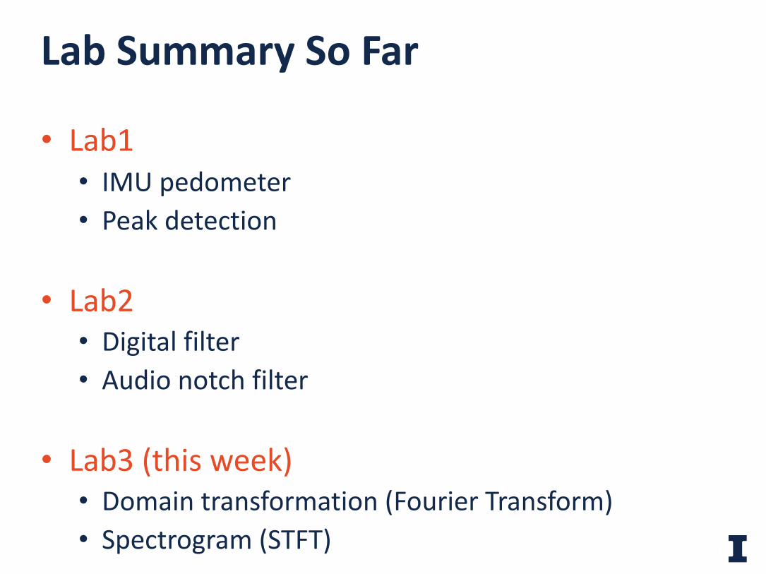
• Lab1• IMU pedometer• Peak detection

• Lab2• Digital filter• Audio notch filter

• Lab3 (this week)• Domain transformation (Fourier Transform)• Spectrogram (STFT)

Lab Summary So Far

2

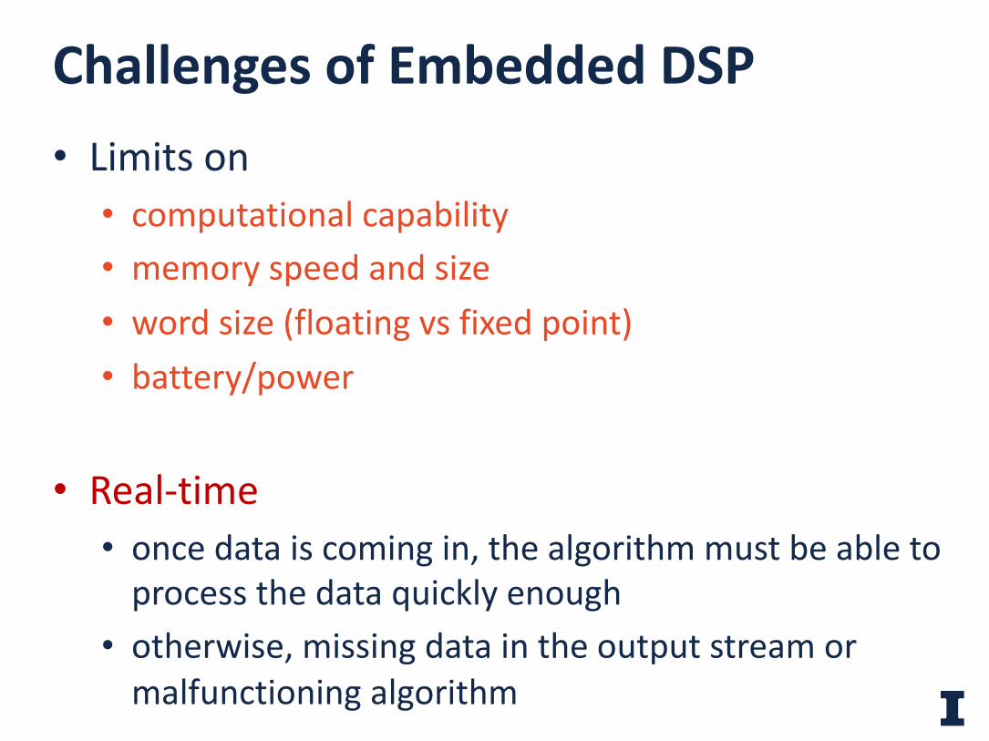
• Limits on• computational capability• memory speed and size• word size (floating vs fixed point)• battery/power

• Real-time• once data is coming in, the algorithm must be able to

process the data quickly enough• otherwise, missing data in the output stream or

malfunctioning algorithm

Challenges of Embedded DSP

3

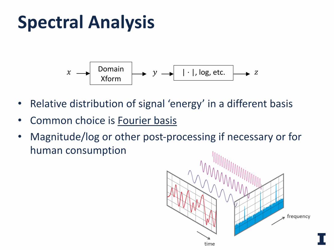
• Relative distribution of signal ‘energy’ in a different basis• Common choice is Fourier basis• Magnitude/log or other post-processing if necessary or for

human consumption

Spectral Analysis

4

𝑥 Domain Xform

𝑦 | · |, log, etc. 𝑧

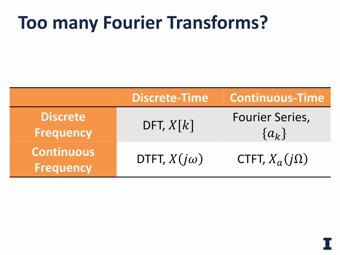
Too many Fourier Transforms?

5

Discrete-Time Continuous-TimeDiscrete

FrequencyContinuous Frequency

DFT, 𝑋[𝑘] Fourier Series, {𝑎*}

DTFT, 𝑋 𝑗𝜔 CTFT, 𝑋. 𝑗Ω

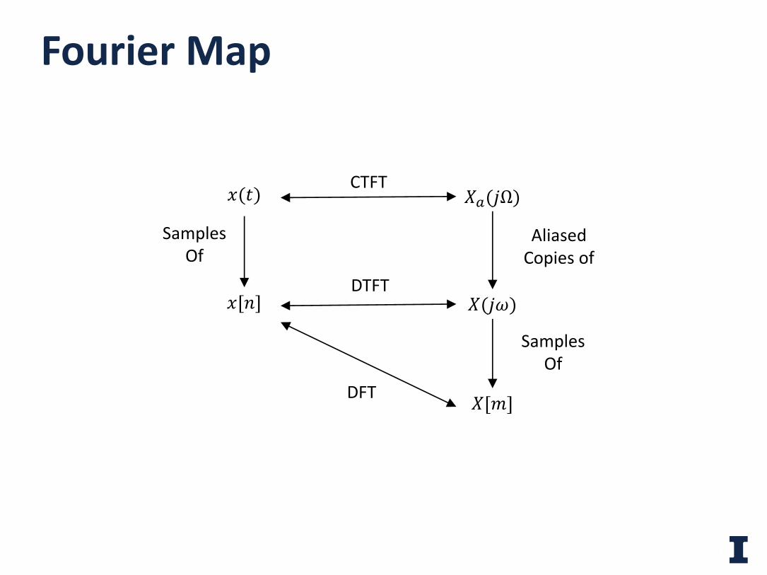
Fourier Map

6

𝑥(𝑡)

𝑥[𝑛]

𝑋.(𝑗Ω)

𝑋(𝑗𝜔)

𝑋[𝑚]

CTFT

DTFT

DFT

Samples Of

Samples Of

Aliased Copies of

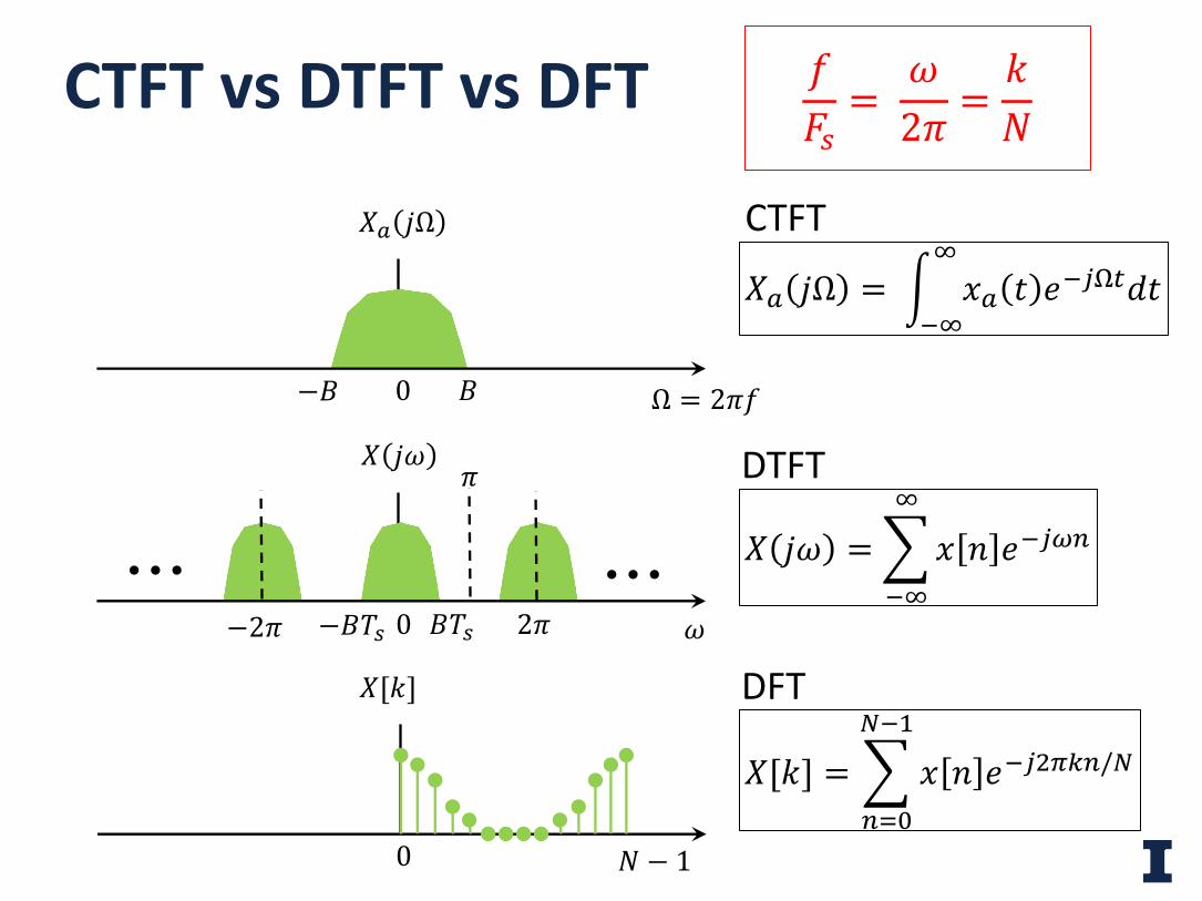
0

𝑋[𝑘]

𝑋[𝑘] = 789:

;<=

𝑥 𝑛 𝑒<?@A*8/;

DFT

𝑁 − 1

CTFT vs DTFT vs DFT

𝑋. 𝑗Ω = F<G

G𝑥. 𝑡 𝑒<?HI𝑑𝑡

0 𝐵−𝐵

𝑋. 𝑗Ω

Ω = 2𝜋𝑓

CTFT

𝑋 𝑗𝜔 =7<G

G

𝑥 𝑛 𝑒<?O8

0 𝐵𝑇Q−𝐵𝑇Q

𝑋 𝑗𝜔

𝜔2𝜋−2𝜋

𝜋

• • •• • •

DTFT

𝑓𝐹Q=

𝜔2𝜋

=𝑘𝑁

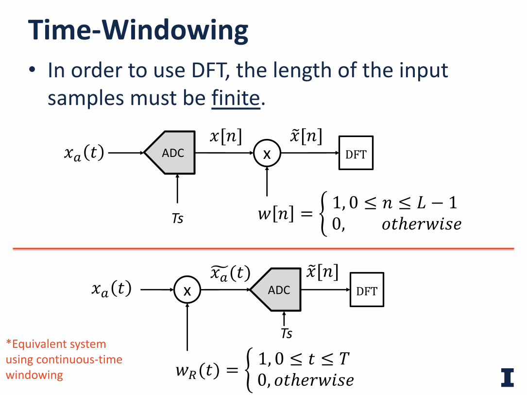
• In order to use DFT, the length of the input samples must be finite.

Time-Windowing

ADC

Ts

𝑥. 𝑡 x DFT𝑥[𝑛] V𝑥[𝑛]

𝑤 𝑛 = X 1, 0 ≤ 𝑛 ≤ 𝐿 − 10, 𝑜𝑡ℎ𝑒𝑟𝑤𝑖𝑠𝑒

ADC

Ts

𝑥. 𝑡 x DFTa𝑥.(𝑡)

𝑤b(𝑡) = X 1, 0 ≤ 𝑡 ≤ 𝑇0, 𝑜𝑡ℎ𝑒𝑟𝑤𝑖𝑠𝑒

V𝑥[𝑛]

*Equivalent systemusing continuous-timewindowing

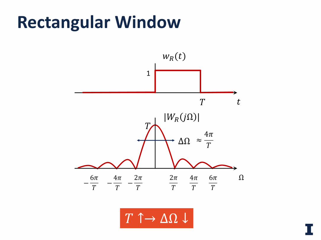
Rectangular Window

9

𝑤b(𝑡)

𝑡

1

𝑇

𝑇 ↑→ ∆Ω ↓

|𝑊b 𝑗Ω |

Ω2𝜋𝑇

4𝜋𝑇

6𝜋𝑇−

6𝜋𝑇 −

4𝜋𝑇

−2𝜋𝑇

𝑇∆Ω ≈

4𝜋𝑇

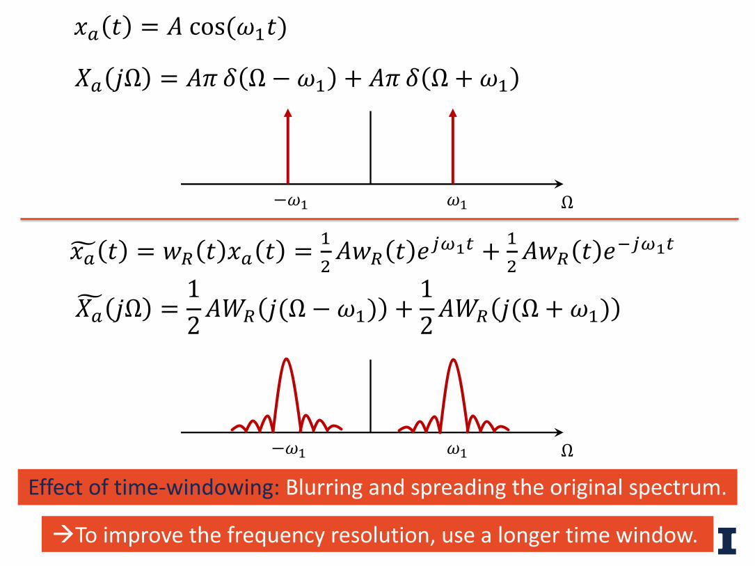
𝑥. 𝑡 = 𝐴 cos(𝜔=𝑡)

𝑋. 𝑗Ω = 𝐴𝜋 𝛿 Ω − 𝜔= + 𝐴𝜋 𝛿 Ω + 𝜔=

a𝑥. 𝑡 = 𝑤b 𝑡 𝑥. 𝑡 = =@𝐴𝑤b 𝑡 𝑒?OrI + =

@𝐴𝑤b 𝑡 𝑒<?OrI

s𝑋. 𝑗Ω =12𝐴𝑊b 𝑗(Ω − 𝜔=) +

12𝐴𝑊b 𝑗(Ω + 𝜔=)

𝜔=−𝜔= Ω

𝜔=−𝜔= Ω

Effect of time-windowing: Blurring and spreading the original spectrum.

àTo improve the frequency resolution, use a longer time window.

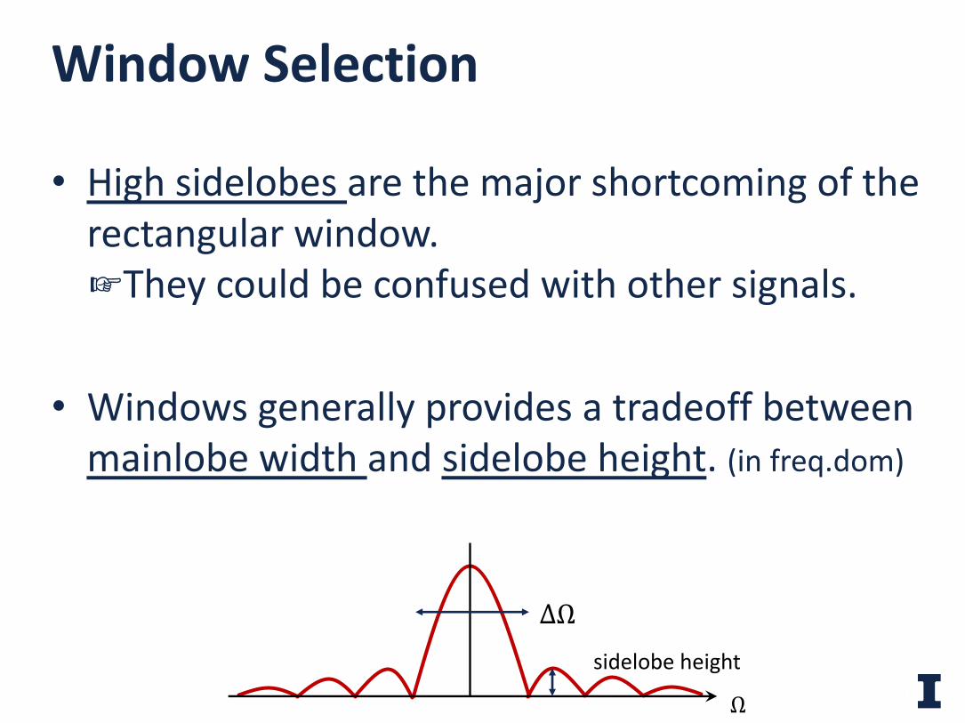
• High sidelobes are the major shortcoming of the rectangular window. ☞They could be confused with other signals.

• Windows generally provides a tradeoff between mainlobe width and sidelobe height. (in freq.dom)

Window Selection

11

∆Ω

Ω

sidelobe height

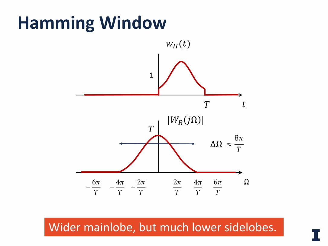
Hamming Window

12

𝑤t(𝑡)

𝑡

1

𝑇

Wider mainlobe, but much lower sidelobes.

|𝑊b 𝑗Ω |

Ω2𝜋𝑇

4𝜋𝑇

6𝜋𝑇−

6𝜋𝑇 −

4𝜋𝑇

−2𝜋𝑇

𝑇∆Ω ≈

8𝜋𝑇

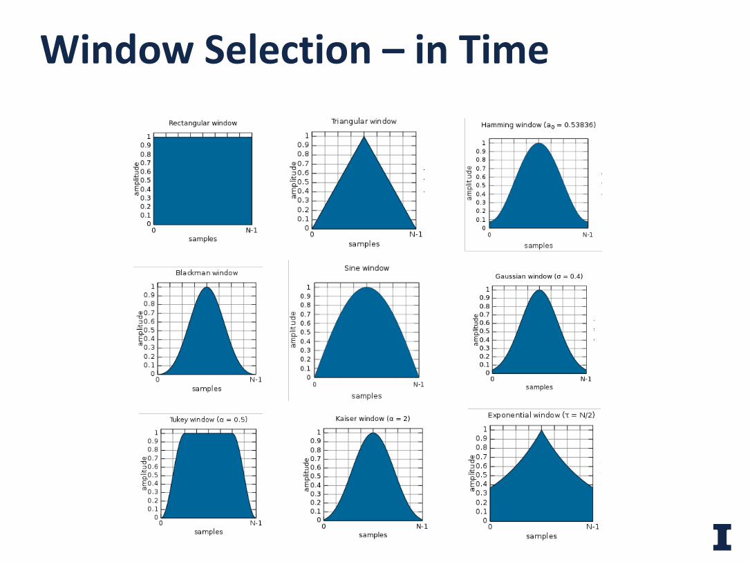
Window Selection – in Time

13

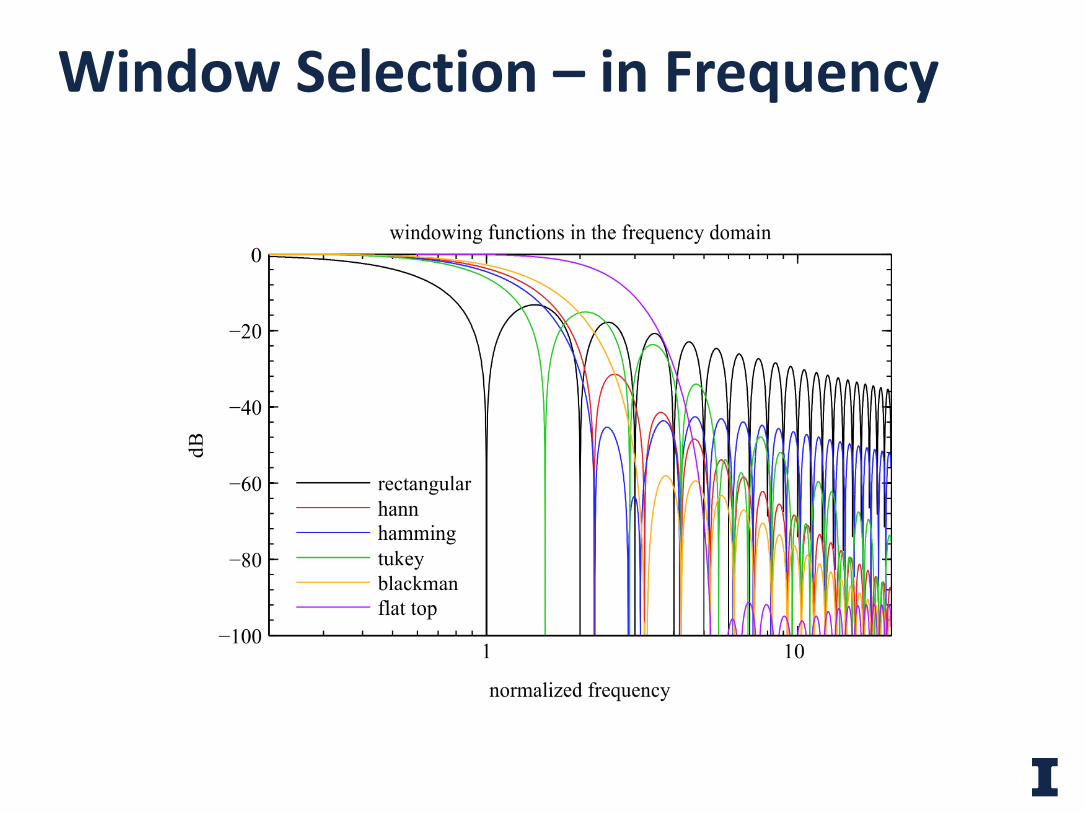
Window Selection – in Frequency

14

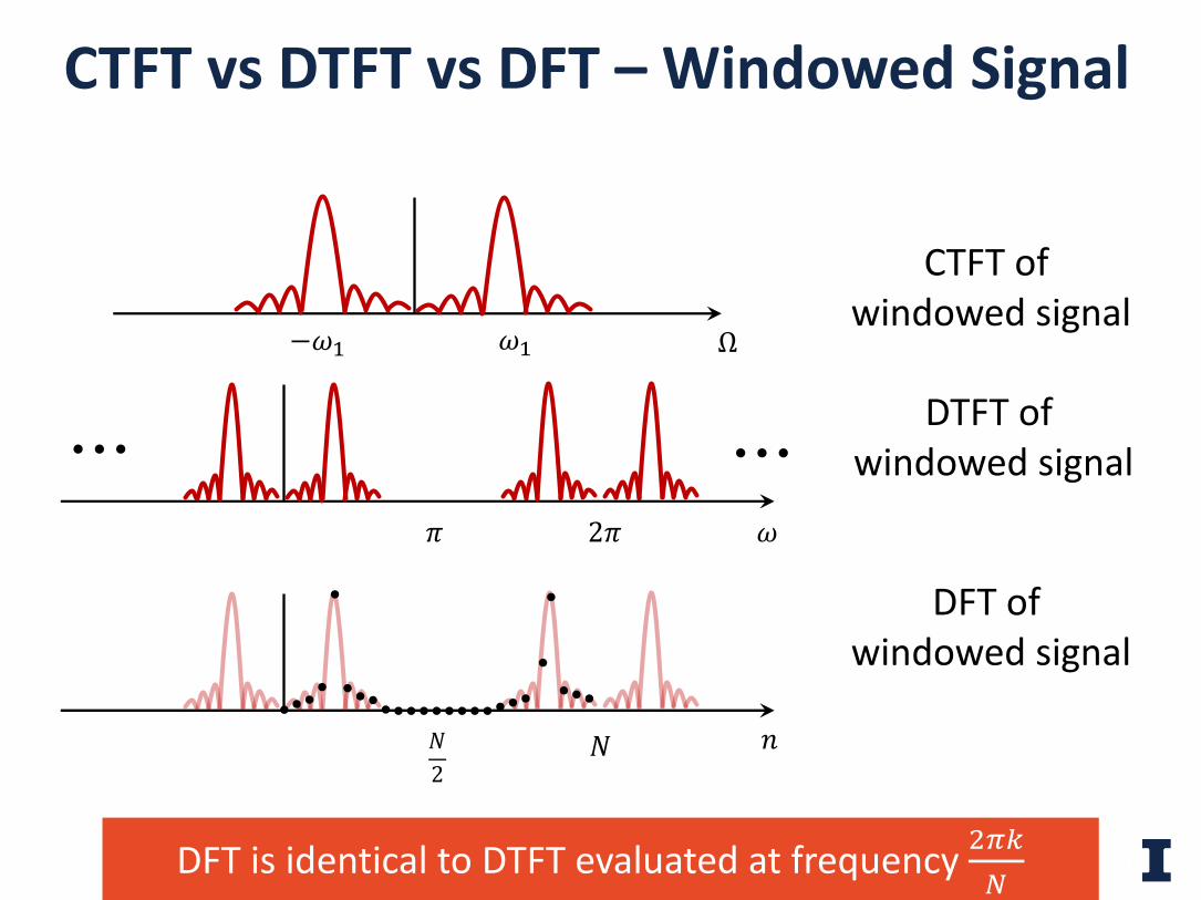
CTFT vs DTFT vs DFT – Windowed Signal

15

𝜔=−𝜔= Ω

𝑛𝑁2

𝑁

• • • • • •

CTFT of windowed signal

DTFT of windowed signal

DFT of windowed signal

𝜔𝜋 2𝜋

DFT is identical to DTFT evaluated at frequency @A*;

• When 𝐿 (window length) < 𝑁(DFT/FFT length), 𝑁 − 𝐿 zero samples are appended to the end of the sequence. This is called zero-padding the signal.

Zero-padding

16

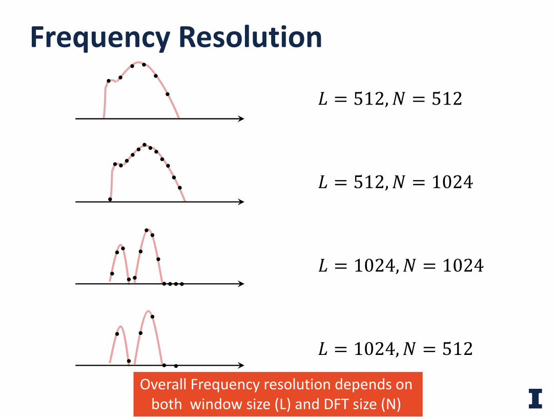
Frequency Resolution

𝐿 = 512,𝑁 = 512

𝐿 = 512,𝑁 = 1024

𝐿 = 1024,𝑁 = 1024

𝐿 = 1024,𝑁 = 512

Overall Frequency resolution depends on both window size (L) and DFT size (N)

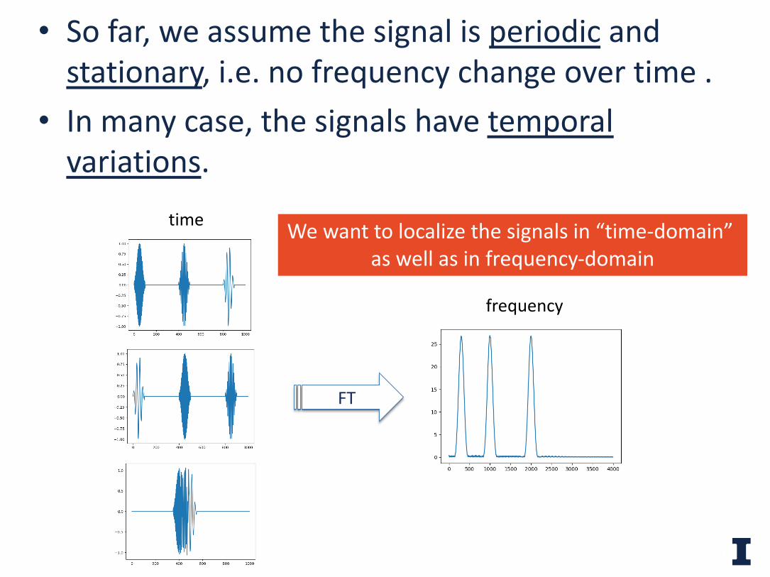
• So far, we assume the signal is periodic and stationary, i.e. no frequency change over time .

• In many case, the signals have temporal variations.

18

FT

time

frequency

We want to localize the signals in “time-domain” as well as in frequency-domain

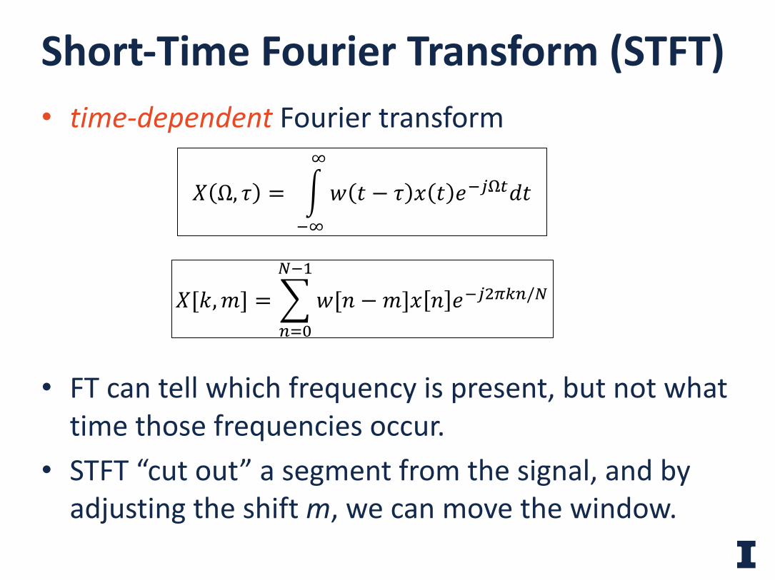
• time-dependent Fourier transform

• FT can tell which frequency is present, but not what time those frequencies occur.

• STFT “cut out” a segment from the signal, and by adjusting the shift m, we can move the window.

Short-Time Fourier Transform (STFT)

19

𝑋 Ω, 𝜏 = F<G

G

𝑤 𝑡 − 𝜏 𝑥 𝑡 𝑒<?HI𝑑𝑡

𝑋[𝑘,𝑚] = 789:

;<=

𝑤[𝑛 −𝑚]𝑥 𝑛 𝑒<?@A*8/;

𝑓

𝑓

𝑓

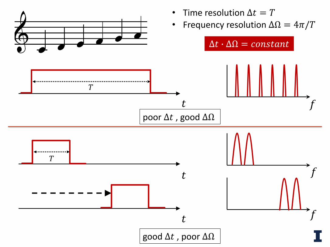
poor Δ𝑡 , good ∆Ω

good Δ𝑡 , poor ∆Ω

• Time resolution Δ𝑡 = 𝑇• Frequency resolution ∆Ω = 4𝜋/𝑇

Δ𝑡 y ∆Ω = 𝑐𝑜𝑛𝑠𝑡𝑎𝑛𝑡

𝑡𝑇

𝑡

𝑡𝑇

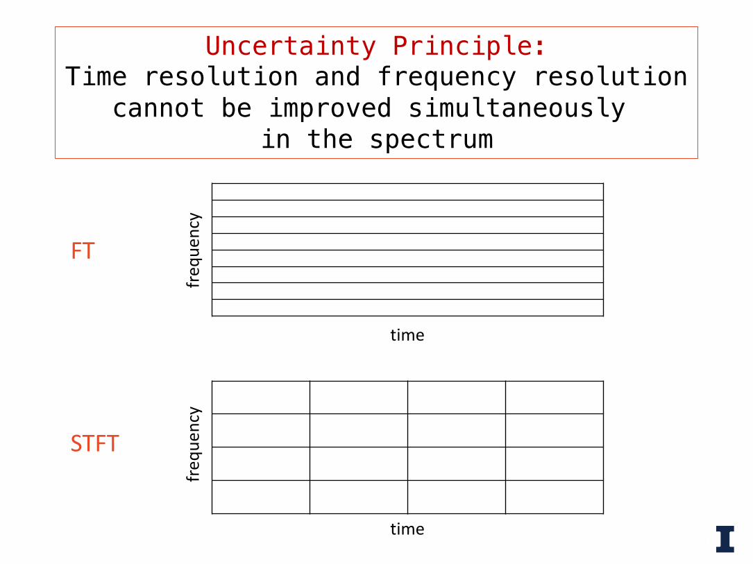
Uncertainty Principle:Time resolution and frequency resolution

cannot be improved simultaneously in the spectrum

time

freq

uenc

y

time

freq

uenc

y

FT

STFT

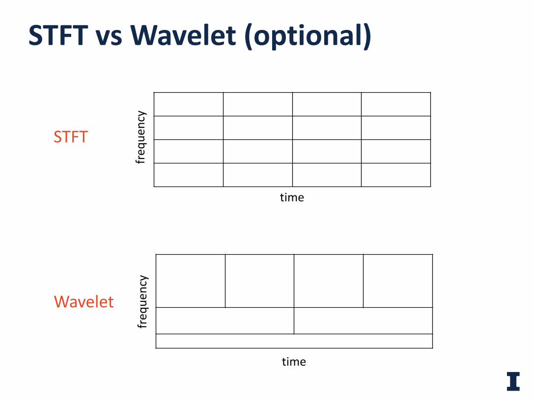
STFT vs Wavelet (optional)

time

freq

uenc

ySTFT

time

freq

uenc

y

Wavelet

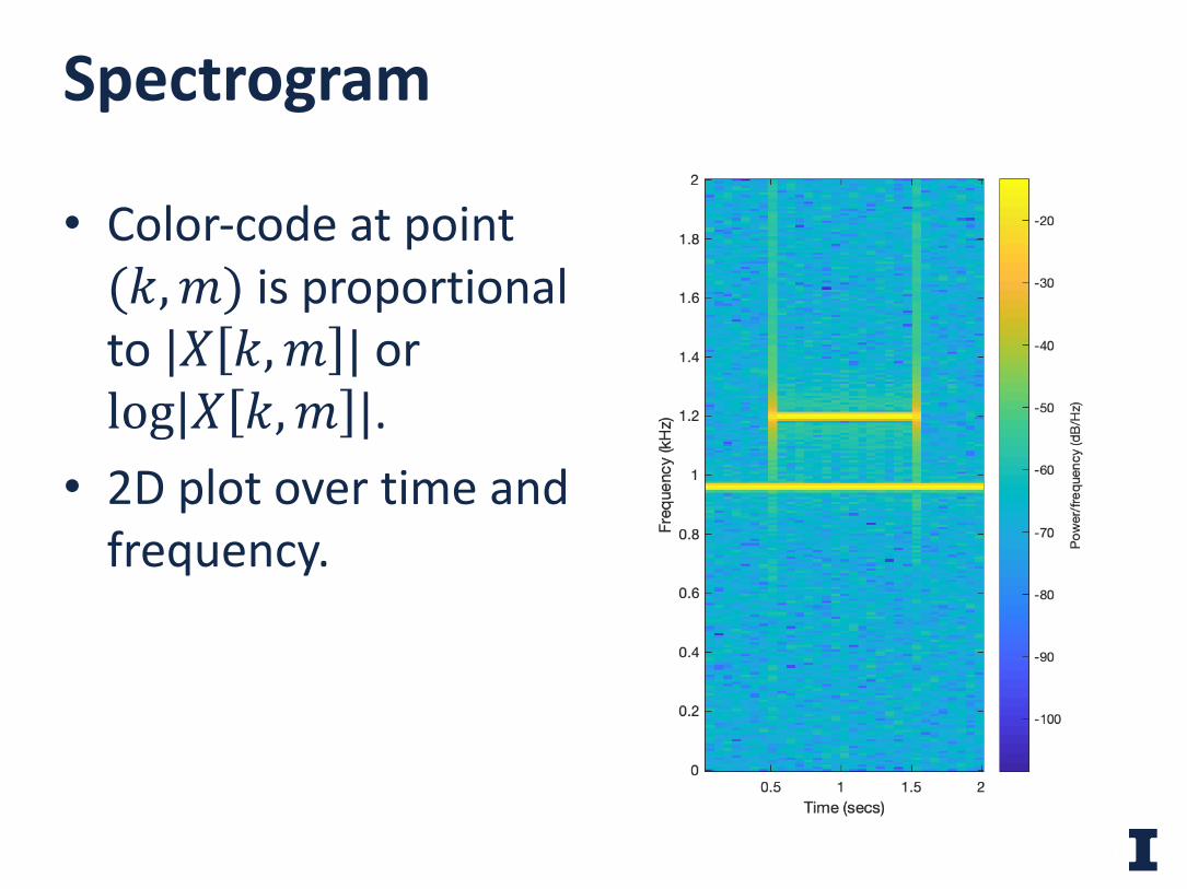
Spectrogram

23

• Color-code at point (𝑘,𝑚) is proportional to |𝑋 𝑘,𝑚 | or log|𝑋 𝑘,𝑚 |.

• 2D plot over time and frequency.

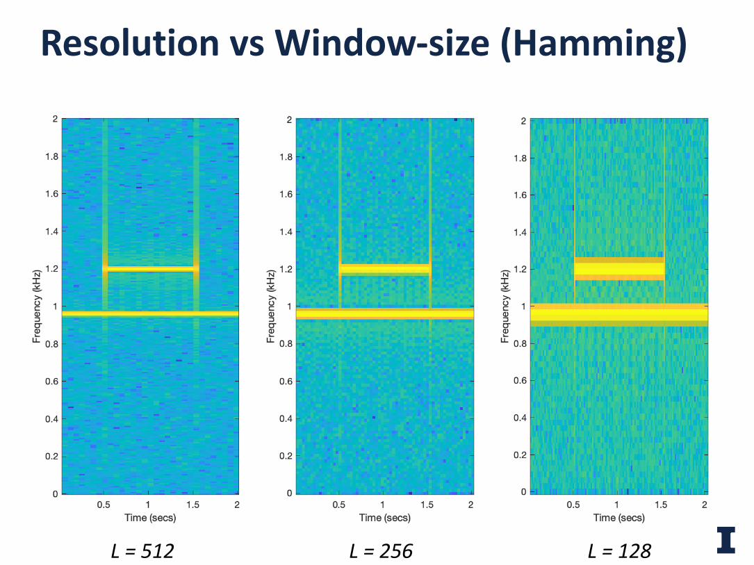
24 L = 512 L = 256 L = 128

Resolution vs Window-size (Hamming)

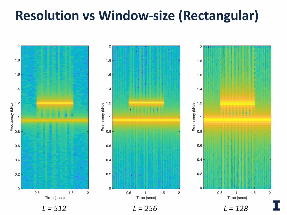
Resolution vs Window-size (Rectangular)

25 L = 512 L = 256 L = 128

• Lab 2: Digital Filtering Quiz/Demo

• Lab 3: Real time spectral analyzer

• Be thinking about Assigned Project Labs

This week…

26