ECE 486: Control Systems

Lecture 14A: Bode Plots for Second-Order Systems

Key Takeaways

This lecture focuses on Bode plots for second order systems.

• Second-order differentiator 𝐺 𝑠 = 𝑠2: Phase is +180o and magnitude has slope +40dB/decade.

• Second-order integrator 𝐺 𝑠 = 1

𝑠2: Phase is -180o and

magnitude has slope -40dB/decade:

• Second-order underdamped 𝐺 𝑠 = 𝑏0𝑠2+2𝜁𝜔𝑛𝑠+𝜔𝑛

2 :

• Magnitude is (approximately) flat up to the corner frequency 𝜔𝑛and rolls off at -40dB/dec at high frequencies.

• Phase plot transitions by ±180𝑜depending on the signs of the coefficients.

• If damping is low (𝜁 ≪ 1) then the plot has a resonant peak of

𝐺 𝑗𝜔𝑛 ≈ 1

2𝜁. The boxed equation should be: 𝐺 𝑗𝜔𝑛 =

𝐺(0)

2𝜁.

2

Problem 1

Sketch approximate, straight-line Bode plots for the following systems:

A)

B)

C)

3

Solution 1A

A)

4

Solution 1B

B)

5

Problem 1A/B

3A/B)

6

Solution 1C

C)

7

ECE 486: Control Systems

Lecture 14B: Frequency Content of Signals

Key Takeaways

Bode plots can be used to gain intuition for how the system will respond to “low frequency” and “high frequency” signals.

The intuition follows from the following facts:

• The steady-state sinusoidal response for a stable system can be computed using the transfer function.

• By linear superposition, if the input is a sum of sinusoids then the steady state response is given by summing the responses due to each input sinusoid.

• General signals can be expressed as a sum of sinusoids using the Fourier Series. Signals can be roughly classified as low or high frequency based on the Fourier Series coefficients.

9

Problem 2

Consider the following first-order system:

Is each input signal below roughly “high frequency” (fast) or “low frequency” slow for this system? Roughly sketch the output.

[Hint: You don’t need to work formally with the Fourier Series. Just consider the time constant of the system.]

10

Input A Input B

Solution 2-Extra Space

% Matlab code

% System

G = tf(2,[1 2]);

% Input A

N=1e3; t1=linspace(0,0.30,N);

u1=t1/0.1; u1(t1>0.10 & t1<=0.20) = 1; idx=find(t1>0.20); u1(idx) =

1-(t1(idx)-0.20)/0.10;

[y1,t1] = lsim(G,u1,t1);

figure(1)

plot(t1,u1,'b',t1,y1,'r--')

% Input B

N=1e3; t2=linspace(0,30,N);

u2=t2/10; u2(t2>10 & t2<=20) = 1; idx=find(t2>20); u2(idx) = 1-

(t2(idx)-20)/10;

[y2,t2] = lsim(G,u2,t2);

figure(2)

plot(t2,u2,'b',t2,y2,'r--')

11

ECE 486: Control Systems

Lecture 14C: Introduction to Bode Plots for

Higher-Order Systems

Key Takeaways

Consider a system whose transfer function is G(s) = G1(s)G2(s).

• The Bode phase plot of G(s) is the sum of the phase plots of G1(s) and G2(s).

• The Bode magnitude plot of G(s) (in dB) is the sum of the magnitude plots of G1(s) and G2(s).

This can be used to draw Bode plots for higher order systems.

13

Problem 3

Sketch approximate, straight-line Bode plots for the following systems:

A)

B)

14

Solution 3A

A)

15

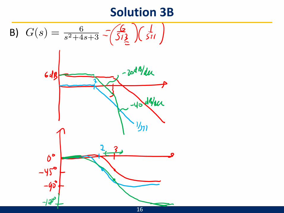
Solution 3B

B)

16

Solution 3-Extra Space

17

18

Problem 4

Consider a feedback system with the plant and controller:

A) What type of controller has the transfer function K(s)?

B) Sketch the Bode magnitude plot of G(s), K(s), and G(s)K(s).

19

Solution 4A

Consider a feedback system with the plant and controller:

A) What type of controller has the transfer function K(s)?

20

Solution 4B

Consider a feedback system with the plant and controller:

B) Sketch the Bode magnitude plot of G(s), K(s), and G(s)K(s).

21