ECE634 – Spring 2021 Feb. 16, 2021 1

ECE 634 – Digital Video SystemsSpring 2021

Fengqing Maggie ZhuAssistant Professor of ECE

MSEE 334zhu0@purdue.edu

Transform Coding

ECE634 – Spring 2021 Feb. 16, 2021 2

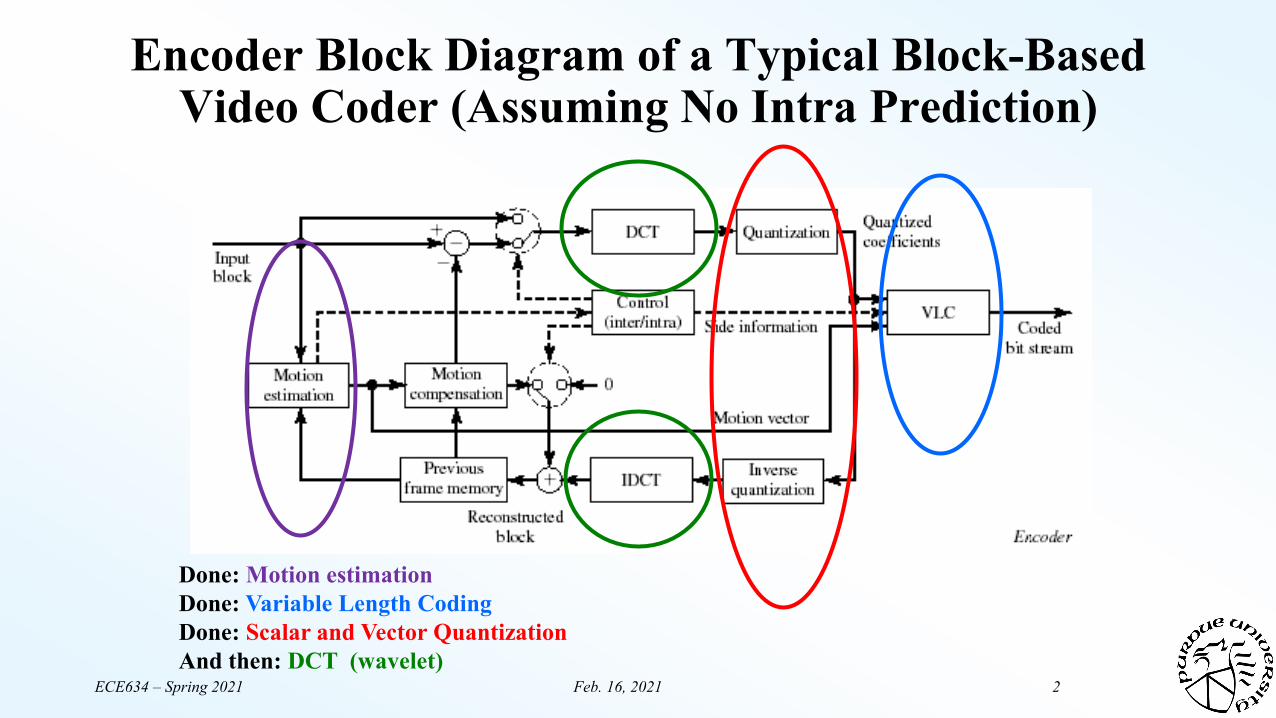
Encoder Block Diagram of a Typical Block-Based Video Coder (Assuming No Intra Prediction)

Done: Motion estimationDone: Variable Length CodingDone: Scalar and Vector QuantizationAnd then: DCT (wavelet)

ECE634 – Spring 2021 Feb. 16, 2021 3

Background Reading (Transform Coding)

• R. J. Clarke, Transform Coding of Images, Academic Press, London, 1985, Chapters 3&4

• W. K. Pratt, Digital Image Processing (2nd ed), Wiley, 1991, Chapter 8• Wang, Ostermann, Zhang, Video Processing and Communications, Prentice

Hall 2002, Section 9.1

ECE634 – Spring 2021 Feb. 16, 2021 4

Transform Coding

• Motivation: – Represent a vector (e.g. a block of image samples) as the superposition of some

typical vectors (block patterns)– Quantize and code the coefficients– Can be thought of as a constrained vector quantizer

+t1 t2 t3 t4 Basis imagesTransform

coefficients(weights)

ECE634 – Spring 2021 Feb. 16, 2021 5

Block Diagram

ECE634 – Spring 2021 Feb. 16, 2021 6

What Transform Basis to Use?

• The transform should– Minimize the correlation among resulting coefficients, so that scalar quantization can

be employed without losing too much in coding efficiency compared to vector quantization

– Compact the energy into as few coefficients as possible• Optimal transform

– Karhunan Loeve Transform (KLT): signal statistics dependent• Suboptimal transform

– Discrete Cosine transform (DCT): nearly as good as KLT for common image signals

ECE634 – Spring 2021 Feb. 16, 2021 7

General Linear Transform

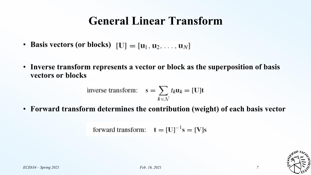
• Basis vectors (or blocks)

• Inverse transform represents a vector or block as the superposition of basis vectors or blocks

• Forward transform determines the contribution (weight) of each basis vector

ECE634 – Spring 2021 Feb. 16, 2021 8

Example

ECE634 – Spring 2021 Feb. 16, 2021 9

Unitary Transform

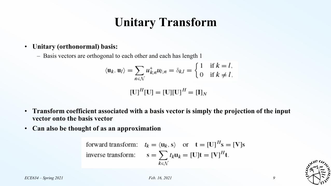
• Unitary (orthonormal) basis: – Basis vectors are orthogonal to each other and each has length 1

• Transform coefficient associated with a basis vector is simply the projection of the input vector onto the basis vector

• Can also be thought of as an approximation

ECE634 – Spring 2021 Feb. 16, 2021 10

Example

ECE634 – Spring 2021 Feb. 16, 2021 11

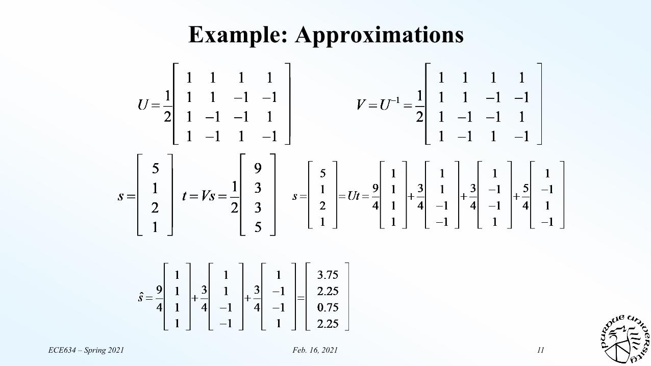
Example: Approximations

ECE634 – Spring 2021 Feb. 16, 2021 12

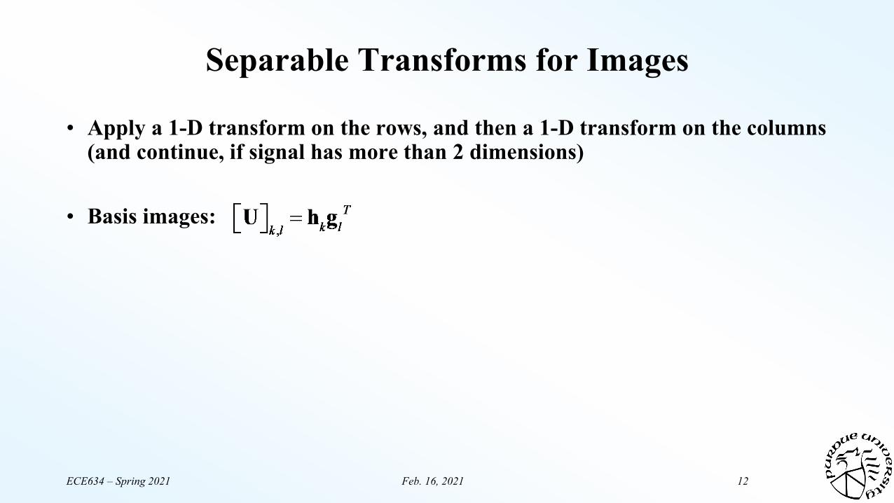
Separable Transforms for Images

• Apply a 1-D transform on the rows, and then a 1-D transform on the columns (and continue, if signal has more than 2 dimensions)

• Basis images:

ECE634 – Spring 2021 Feb. 16, 2021 13

Transform Design

• What are desirable properties of a transform for image and video?– Nearly decorrelating – improves efficiency of scalar quantizer– High energy compaction – a few large coefficients to send– Easy to compute (few operations)– Separable – compute 1-D transform first on rows, then on columns

• What size transform should we use?– Entire image? Small? – 2-D (on an image) or 3-D (incorporating time also)?

ECE634 – Spring 2021 Feb. 16, 2021 14

Karhunen Loève Transform (KLT)

• Optimal transform• Requires statistics of the input source

– Known covariance function

• Coefficients are completely uncorrelated• The best energy compaction

– Sort coefficients from largest to smallest expected squared magnitude; then the sum of the energies of the first M coefficients is as large as possible

• No computationally efficient algorithm

• We’ll derive it later

ECE634 – Spring 2021 Feb. 16, 2021 15

Other Transform Bases

• Optimal transform – Karhunen Loève Transform (KLT): Depends on the signal statistics

• Suboptimal transforms – many available!– Discrete Fourier Transform (DFT): complex values; discontinuities– Discrete Cosine transform (DCT): nearly as good as KLT for common image signals– Hadamard and Haar: basis functions contain only +1,0,-1

ECE634 – Spring 2021 Feb. 16, 2021 16

DFT vs. DCT

• DFT is complex; DCT is real• Consider continuous signal, sampled over window of length N• When applying DFT, transform-domain is not the isolated segment. Instead,

that sampled signal gets repeated. If left side is not same value as right side, severe discontinuities

• DCT equivalent to “folding” signal and applying DFT

ECE634 – Spring 2021 Feb. 16, 2021 17

Discrete Cosine Transform (8 x 8 Basis Image)

1-D Forward Transform

1-D Inverse Transform

Example in Matlab:D=dctmtx(8);X=zeros(8);X(4,3)=1;Basis=D’*X*D;

64 Basis Functions of an 8-by-8 Matrix

ECE634 – Spring 2021 Feb. 16, 2021 18

Energy/Variance Distribution of DCT Coefficients in Typical Images

Zigzag order; low horizontal and low vertical indices are earlier

ECE634 – Spring 2021 Feb. 16, 2021 19

Images Approximated by Different Number of DCT Coefficients

Original

With 8/64Coefficients

With 16/64Coefficients

With 4/64Coefficients

ECE634 – Spring 2021 Feb. 16, 2021 20

Bit Allocation for Transform Coding(Outline)

• Assumptions: – 1-D transform; Scalar quantization with MMSE quantizer; Fixed-length coding

• Goal: what is the average distortion and bit-rate per sample

• Computing distortion• Optimal bit allocation among the N transform coefficients

– High rate approximation• Performance improvement relative to pixel-based coding• Examples

• Optimal transform design

ECE634 – Spring 2021 Feb. 16, 2021 21

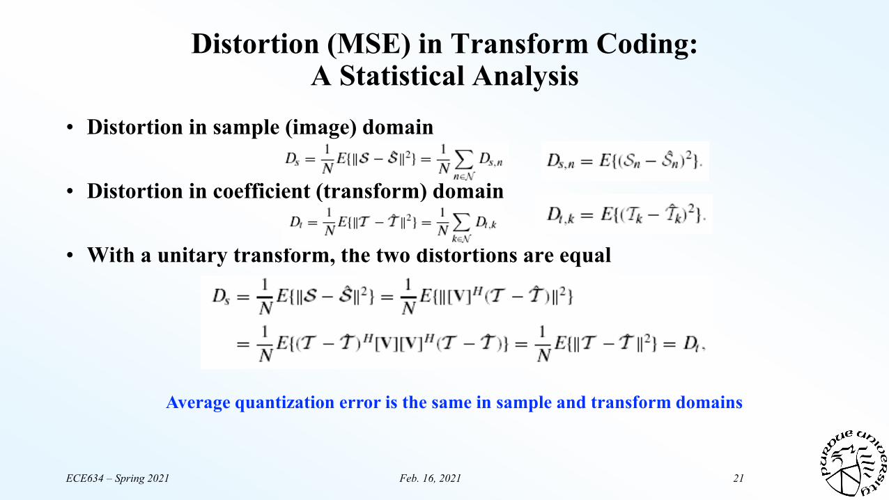
Distortion (MSE) in Transform Coding: A Statistical Analysis

• Distortion in sample (image) domain

• Distortion in coefficient (transform) domain

• With a unitary transform, the two distortions are equal

Average quantization error is the same in sample and transform domains

ECE634 – Spring 2021 Feb. 16, 2021 22

Modeling Distortion Due to Coefficient Quantization

• How much distortion is introduced by quantizing the k-th transform coefficient?

• Use a high-resolution approximation of scalar quantization – MMSE quantizer; each coefficient is quantized with high rate; pdf in each

quantization bin is nearly flat

Depends on the pdf of the k-th coefficient.

One coefficient

Average overall coefficients

ECE634 – Spring 2021 Feb. 16, 2021 23

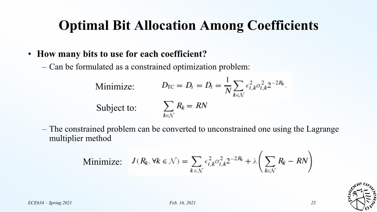
Optimal Bit Allocation Among Coefficients

• How many bits to use for each coefficient? – Can be formulated as a constrained optimization problem:

– The constrained problem can be converted to unconstrained one using the Lagrange multiplier method

Minimize:

Subject to:

Minimize:

ECE634 – Spring 2021 Feb. 16, 2021 24

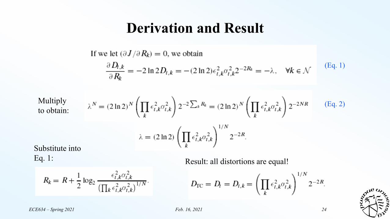
Derivation and Result

Multiplyto obtain:

Substitute intoEq. 1: Result: all distortions are equal!

(Eq. 1)

(Eq. 2)

ECE634 – Spring 2021 Feb. 16, 2021 25

Implication of Optimal Bit Allocation

• Bit rate for a coefficient proportional to its variance (energy)

• Distortion is equalized among all coefficients and depends on the geometric mean of the coefficient variances

Geometric mean

ECE634 – Spring 2021 Feb. 16, 2021 26

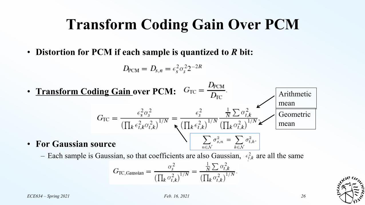
Transform Coding Gain Over PCM

• Distortion for PCM if each sample is quantized to R bit:

• Transform Coding Gain over PCM:

• For Gaussian source – Each sample is Gaussian, so that coefficients are also Gaussian, are all the same

Arithmetic meanGeometric mean

ECE634 – Spring 2021 Feb. 16, 2021 27

ExampleDetermine the optimal bit allocation for a given average bit rate of R, and the corresponding TC gain for coding 2x2 image block using 2x2 DCT. Assuming the image is a stationary Gaussian process with variance 𝜎𝜎𝑠𝑠2 and inter-sample correlation as shown below.

= 0.95

2R = 2 1sσ =

ECE634 – Spring 2021 Feb. 16, 2021 28

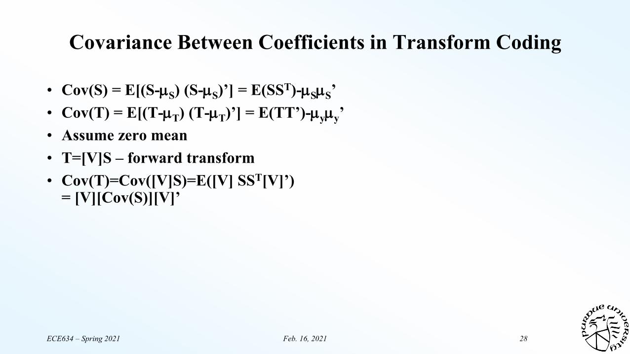
Covariance Between Coefficients in Transform Coding

• Cov(S) = E[(S-µS) (S-µS)’] = E(SST)-µSµS’• Cov(T) = E[(T-µT) (T-µT)’] = E(TT’)-µyµy’• Assume zero mean• T=[V]S – forward transform• Cov(T)=Cov([V]S)=E([V] SST[V]’)

= [V][Cov(S)][V]’

ECE634 – Spring 2021 Feb. 16, 2021 29

Example Continued(Convert 2x2 into 4x1)

• Covariance matrix(assume zero mean)

• DCT basis images

• Equivalent transform matrix

ECE634 – Spring 2021 Feb. 16, 2021 30

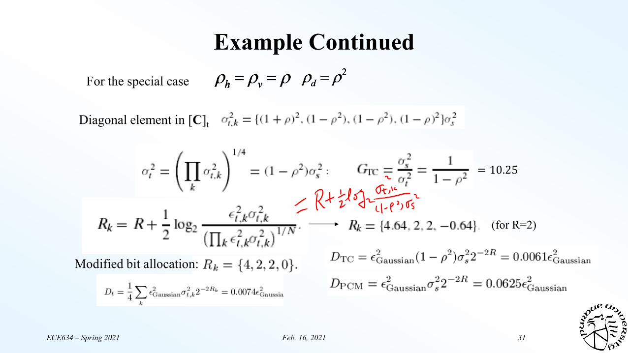
Example Continued

ECE634 – Spring 2021 Feb. 16, 2021 31

Example Continued

(for R=2)

Diagonal element in [C]t

Modified bit allocation:

For the special case

= 10.25

ECE634 – Spring 2021 Feb. 16, 2021 32

Optimal Transform

• Approach 1: Minimize the MSE introduced if we omit a coefficient– Start with smallest coefficient, then next, etc

• Approach 2: Minimize the correlation between different transform coefficients

• Approach 3: Maximize the transform coding gain

• All lead to same answer (assuming Gaussian source): Karhunen LoeveTransform (KLT)

ECE634 – Spring 2021 Feb. 16, 2021 33

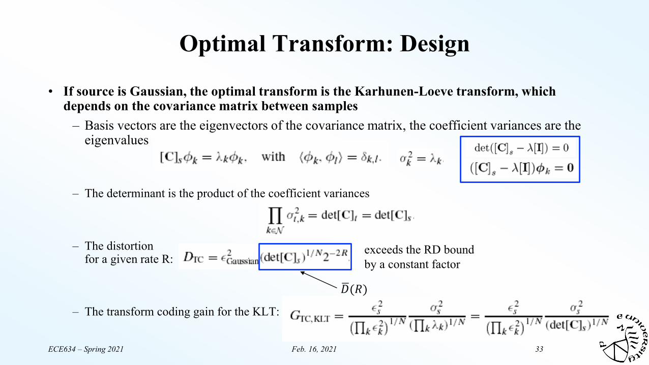
• If source is Gaussian, the optimal transform is the Karhunen-Loeve transform, which depends on the covariance matrix between samples

– Basis vectors are the eigenvectors of the covariance matrix, the coefficient variances are the eigenvalues

– The determinant is the product of the coefficient variances

– The distortionfor a given rate R:

– The transform coding gain for the KLT:

Optimal Transform: Design

exceeds the RD bound by a constant factor

�𝐷𝐷(𝑅𝑅)

ECE634 – Spring 2021 Feb. 16, 2021 34

What Would Be Necessary To Implement in a Real System?

• Estimate the data covariance matrix– For both row and column!

• Compute eigenvectors to generate basis vectors• Associate this KLT with the image

– Either when stored, or transmitted

• But the relative gains for typical images is small

ECE634 – Spring 2021 Feb. 16, 2021 35

Example Gains: 1st Order Markov Source, Rho=0.91

• Define efficiency to be the amount of source energy contained in all coefficients up to and including coefficient i

1 2 3 4 5 6 7 8KLT 79.5 91.1 94.8 96.7 97.9 98.7 99.4 100DCT 79.3 90.9 94.8 96.7 97.9 98.7 99.4 100Hadamard

79.3 89.3 92.7 95.5 96.7 97.9 99 100

DST 73.6 84.3 92.5 95.0 97.4 98.4 99.4 100

From R. J. Clarke, Transform coding of images, Prentice Hall, 1985. Chapter 3.

ECE634 – Spring 2021 Feb. 16, 2021 36

Properties of KLT

• The optimal transform for Gaussian sources• Nearly optimal transform for non-Gaussian sources

• Minimal approximation error for K<N coefficients among all unitary transforms

• KLT has highest energy compaction• Coefficients are uncorrelated

• Requires a stationary source with known covariance matrix – most sources vary spatially and temporally

• No fast algorithms

ECE634 – Spring 2021 Feb. 16, 2021 37

Example

• Determine the KLT for the 2x2 image block in the previous example

Determine the eigenvalues by solving:

Determine the eigenvectors by solving

(same as the coefficient variances with DCT)

Resulting transform is the DCT (because this is a 2*2 example!!)

ECE634 – Spring 2021 Feb. 16, 2021 38

Example: JPEG Image Coder

• Joint Photographic Expert Group• Uses 8x8 DCT• Each coefficient is quantized using a uniform quantizer• Step sizes vary based on coefficient variances and their visual importance• Quantized coefficients are converted into binary bitstreams using run-length

coding plus Huffman coding

ECE634 – Spring 2021 Feb. 16, 2021 39

Perceptual based quantization matrix: Zig-zag ordering of DCT coefficients:

Run-length coding example:

JPEG: A Bit More Detail

ECE634 – Spring 2021 Feb. 16, 2021 40

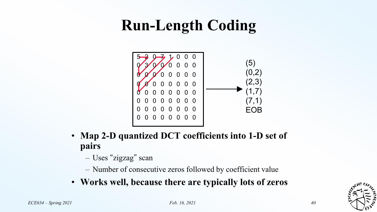
5 2 0 7 1 00 00 3 0 0 0 00 00 0 0 0 0 00 00 0 0 0 0 00 00 0 0 0 0 00 00 0 0 0 0 00 00 0 0 0 0 00 00 0 0 0 0 00 0

Run-Length Coding

• Map 2-D quantized DCT coefficients into 1-D set of pairs

– Uses “zigzag” scan– Number of consecutive zeros followed by coefficient value

• Works well, because there are typically lots of zeros

(5)(0,2)(2,3)(1,7)(7,1)EOB

ECE634 – Spring 2021 Feb. 16, 2021 41

Practice ProblemConsider applying transform coding to each 2x2 block of an image, using a 2x2 DCT. Assume the image is a stationary Gaussian process with variance 𝜎𝜎𝑠𝑠2 and that the correlation coefficients show below. Determine the optimal bit allocation for a given average bit rate of R=2 bits/pixel, and the corresponding distortion. Compare this coder with a PCM coder that directly quantizes each sample using optimal scalar quantizer.

𝜌𝜌ℎ = 𝜌𝜌𝑣𝑣 = 𝜌𝜌𝑑𝑑 = 𝜌𝜌 = 0.95

ECE634 – Spring 2021 Feb. 16, 2021 42

ECE634 – Spring 2021 Feb. 16, 2021 4343