Efficient Mesh Deformation Using Tetrahedron Control Mesh
Jin Huang∗ Lu Chen† Xinguo Liu ‡ § Hujun Bao¶
State Key Lab of CAD&CG, Zhejiang UniversityHangzhou, P. R. China
Abstract
It is a challenging problem to interactively deform densely sam-pled complex objects. This paper proposed an easy but efficientapproach to it by using coarse control meshes to embed the tar-get objects. The control mesh can be efficiently deformed by var-ious existing methods, and then the target object can be accord-ingly deformed by interpolation. One of the most simplest inter-polation methods is to use the barycentric coordinates, which how-ever generates apparent first-order discontinuity artifacts across theboundary due to its piecewise linear property. To avoid such ar-tifacts, this paper introduced a modified barycentric interpolation(modified-BI) technique. The central idea is to add a local trans-formation at each control vertex for interpolation, so that we canminimize the first-order discontinuity by optimizing the local trans-formations. We also minimize the second order derivatives of theinterpolation function to avoid undesired vibrations. While focuson deforming 3D objects embedded in tetrahedron meshes, the pro-posed method is applicable to 2D image objects embed in planartriangular meshes. The experimental results in both 2D and 3Ddemonstrated the success and advantages of the proposed method.
CR Categories: I.3.5 [Computational Geometry and ObjectModeling]—Curve, surface, solid, and object representations;
Highly complex models become more and more popular and bringbig challenges for nowadays geometry processing algorithms. Toaddress the problem, people create a sparse control mesh or vol-umetric control lattice to embed and manipulate the target modelby using various interpolation techniques. Free form deformation(FFD) methods adopt spline functions to achieve smooth interpo-lation results [Sederberg and Parry 1986]. Such smooth interpola-tion can be achieved alternatively by using mean value coordinate(MVC) [Floater 2003; Ju et al. 2005], which doesn’t need a volu-metric control lattice. While high quality results are achieved, theevaluation procedure requires the information of a relative largestencil of neighborhoods or even the whole control mesh, whichis not suitable for GPU implementation.
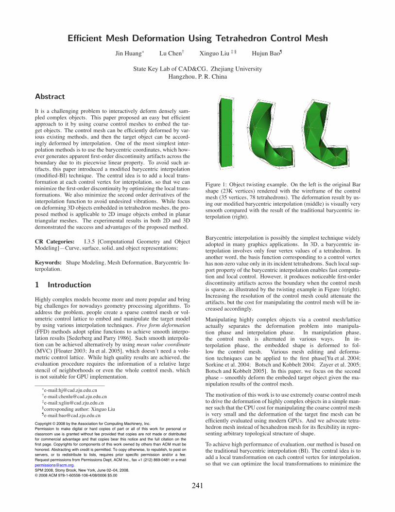
Figure 1: Object twisting example. On the left is the original Barshape (23K vertices) rendered with the wireframe of the controlmesh (35 vertices, 78 tetrahedrons). The deformation result by us-ing our modified barycentric interpolation (middle) is visually verysmooth compared with the result of the traditional barycentric in-terpolation (right).
Barycentric interpolation is possibly the simplest technique widelyadopted in many graphics applications. In 3D, a barycentric in-terpolation involves only four vertex values of a tetrahedron. Inanother word, the basis function corresponding to a control vertexhas non-zero value only in its incident tetrahedrons. Such local sup-port property of the barycentric interpolation enables fast computa-tion and local control. However, it produces noticeable first-orderdiscontinuity artifacts across the boundary when the control meshis sparse, as illustrated by the twisting example in Figure 1(right).Increasing the resolution of the control mesh could attenuate theartifacts, but the cost for manipulating the control mesh will be in-creased accordingly.
Manipulating highly complex objects via a control mesh/latticeactually separates the deformation problem into manipula-tion phase and interpolation phase. In manipulation phase,the control mesh is alternated in various ways. In in-terpolation phase, the embedded shape is deformed to fol-low the control mesh. Various mesh editing and deforma-tion techniques can be applied to the first phase[Yu et al. 2004;Sorkine et al. 2004; Botsch and Kobbelt 2004; Zayer et al. 2005;Botsch and Kobbelt 2005]. In this paper, we focus on the secondphase – smoothly deform the embeded target object given the ma-nipulation results of the control mesh.
The motivation of this work is to use extremely coarse control meshto drive the deformation of highly complex objects in a simple man-ner such that the CPU cost for manipulating the coarse control meshis very small and the deformation of the target fine mesh can beefficiently evaluated using modern GPUs. And we advocate tetra-hedron mesh instead of hexahedron mesh for its flexibility in repre-senting arbitrary topological structure of shape.
To achieve high performance of evaluation, our method is based onthe traditional barycentric interpolation (BI). The central idea is toadd a local transformation on each control vertex for interpolation,so that we can optimize the local transformations to minimize the
241
first-order discontinuity. We also minimize the second order deriva-tives of the interpolation function to avoid undesired vibrations.
There are several advantages in our modified barycentric interpola-tion techniques: (1) the positions of the control vertices are repro-duced; (2) it can generate visually smooth interpolation results evenwith extremely coarse control mesh; (3) it can be locally evaluated,implemented in GPU achieving high performance.
Though the first-order continuity is not guaranteed theoretically, ourmethod greatly improves the smoothness of the deformation resultsas numerically validated in our experiments. The main contributionof this paper is an efficient mesh deformation scheme which uses acoarse control mesh and the novel modified barycentric interpola-tion technique.
2 Related Work
Our work is closely related to many shape deformation techniques.Theoretically speaking, any deformation can be achieved by manu-ally manipulating individual vertices, which is however impracticaldue to the complexity of meshes in practice. FFD techniquesreduce the manual work by embedding the complex shape in a rel-atively simple control lattice [Sederberg and Parry 1986]. The usercan control FFD results by various controls[Milliron et al. 2002],such as lattice [Sederberg and Parry 1986; Coquillart 1990;MacCracken and Joy 1996], feature lines [Beier and Neely 1992],control curves [Barr 1984; Singh and Fiume 1998;Kho and Garland 2005], points [Hsu et al. 1992] and sur-faces [Feng et al. 1996]. Then the embedded shape is deformedvia interpolation. Mean value coordinates (MVC) [Ju et al. 2005]provides an alternative interpolation method, which uses a coarsecontrol surface instead of a control lattice. However, MVC isinversely proportional to the Euclidean distance, which causesundesired artifacts in nearby components, as exemplified byFigure 2(e) in [Joshi et al. 2007]. The positive MVC avoids thisproblem by culling the contributions from invisible surfaces[Lipman et al. 2007]. Though the positive MVC can be fastcomputed in GPU, the interpolation procedure is not suitable forGPU implementation.
Gradient domain deformation technique refers to a fam-ily of methods recently developed after the work ofpoisson mesh editing[Yu et al. 2004], Laplacian meshediting[Alexa 2003; Sorkine et al. 2004] and deformation transfer[Sumner and Popovic 2004], which basically reconstruct the de-formed shape from the alternated gradients or Laplacian/differentialcoordinates, preserving surface details. By far, several new rep-resentation for encoding surface and volumetric details havebeen proposed, such as graph-Laplacian [Zhou et al. 2005],rotation-invariant [Lipman et al. 2005] and edge-based differen-tial coordinates [Huang et al. 2006b; Sorkine and Alexa 2007].Gradient domain techniques were also adopted in sketch-baseduser interface [Zhou et al. 2005; Nealen et al. 2005], shape inter-polation [Xu et al. 2005] and mesh-based IK [Sumner et al. 2005;Der et al. 2006]. In addition, several dimension reduction methodsbased on mean value coordinates [Huang et al. 2006c] and skeletonmodels [Yoshizawa et al. 2007; Weber et al. 2007; Shi et al. 2007]were developed for acceleration and robustness.
Our method in this paper is also applicable to de-forming 2D image objects [Beier and Neely 1992;Cohen-Or et al. 1998; Igarashi et al. 2005]. Recently, Schaefer etal. [Schaefer et al. 2006] proposed an novel image deformationalgorithm using moving least squares (MLS). This techniqueshares some similarity with ours in using affine transformationsto deform the image content as-rigid-as-possible. But ours uses asparse control mesh, and works for both 2D and 3D objects.
In the rest of this paper, we will first introduce the modi-fied barycentric interpolation (modified-BI) method in Section 3;then present an energy minimization framework for constructingmodified-BI in Section 4; then combine the modified-BI with sev-eral existing deformation techniques and present the experimentsresults in Section 5. Finally, we conclude this paper with some dis-cussions on future work in Section 6.
3 Modified Barycentric Interpolation(modified-BI)
Let Ω be an object in Rd , d = 2 or 3, and Φ = (U,T ) be a finiteelement tessellation of Ω, where U = (u1, . . . ,un) denotes the ver-tex set and T = (t1, . . . , tm) denotes the element set. we call Φ thecontrol mesh of the object, and U the control vertices. Φ is a planartriangle mesh for d = 2, and a tetrahedron mesh for d = 3.
Consider a deformation function x(u): Ω→ Rd , with known valuesat the vertices x(ui) = xi,∀ ui ∈U . The simplest way to define thefunction value for the interior of an element is by using barycentricinterpolation:
x(u) =n
∑i=1
φi(u)xi, (1)
where φi(u) is the barycentric coordinate basis function, which sat-isfies ∑n
i=1 φi(u) ≡ 1 and φi(u j) = δi j .
The above barycentric interpolation is simple and has many goodproperties, such as local support and linear reproduction. It how-ever often generates non-smooth (first-order discontinuity) artifactsacross the element boundaries, as shown in Figure 1 (right). Toaddress the problem, we introduce an affine transformation at eachcontrol vertex, which can change the deformation gradient to beas close as possible to each other at the boundaries. This modifiedbarycentric interpolation (modified-BI) is formulated as follows:
x(u) =n
∑i=1
φi(u)(xi +Mi(u−ui)) , (2)
where Mi is the transformation matrix associated with vertex ui tobe determined.
It is worth pointing out that the traditional barycentric interpolationis a special case of the modified-BI with all Mi = 0. An importantproperty of our modification is that, for any set of {Mi}, it stillfollows the control values, i.e.
x(uk) =n
∑i=1
φi(uk)(xi +Mi(uk −ui)) = xk, ∀ uk ∈U.
This property is critical for deformation application.
By the linear reproduction and partition of unit property of thebarycentric coordinate φi(u), the modified-BI function x(u) doesn’tchange if we add an arbitrary local transformation T to all Mi,shown as follows:
For later convenience, we arrange all Mi continuously into a d ∗d ∗n dimension vector m, all control value xi into a d ∗ n dimension
242
(a) Original (b) BI (c) s = 1,θ = 60◦ (d) s = 0.8,θ = 26◦ (e) s = 0.5,θ = 0◦
Figure 2: Function of the local transformation in 2D. (a) original image and the control mesh shown in red wires; (b) deformation resultby manipulating the control points in the second outer loop and using barycentric interpolation (BI); (c) & (d) & (e): deformation resultsby adding a local transformation M to the central control point marked by a big white dot and using modified-BI. M takes the form M =s Rθ − I2×2, where Rθ denotes a 2D rotation of angle θ .
vector x, and rewrite the modified interpolation function x(u) in thefollowing matrix form:
x(u) = A(u)m+B(u)x, (4)
where A(u) and B(u) are respectively d × (d ∗ d ∗ n) matrix andd × (d ∗ n) matrix. A(u)’s elements are u’s second-order polyno-mials formed by the ui, φi(u) and u, while B(u)’s elements are u’sfirst-order polynomials formed by φi(u). Therefore, the second or-
der derivatives ∂ 2A(u)∂u∂u form a constant order-4 tensor, the first order
derivatives ∂B(u)∂u form a constant order-3 tensor, and the second
order derivatives ∂ 2B(u)∂u∂u are all zero.
In Equation (2) of modified-BI, Mi is a local transformation in thevicinity of vertex ui. The 2D examples in Figure 2 demonstrate howthe local transformations affect the interpolation results. Only onelocal transformation is added at the center point of the control meshfor clarity. The visually best interpolation result is achieved in Fig-ure 2(c). In the next section, we propose an optimization method tofind the optimal local transformations that produce visually plausi-ble smooth interpolation results.
4 Optimization
We first introduce our energy terms used for optimizing the localtransformations. The first one measures the gradient discontinuity(first-order) while the second one measures the vibration (second-order) of the deformation.
4.1 Discontinuity Energy
Recall that φi(u) are piecewise linear basis functions of u, the defor-mation gradient of x(u) may not be continuous across the boundaryof two adjacent elements. Consider two adjacent elements, Ti andTj , which share a boundary i ↔ j. We measure the discontinuity byintegrating the squared difference of the deformation gradient overboundary i ↔ j as follows:
Ei↔ j(x) =∫
i↔ j
∥∥∥∇x(u)|i→ j − ∇x(u)| j→i
∥∥∥2
Fdσ , (5)
where i → j denotes the boundary at the side of Ti, j → i denotesthe boundary at the side of Tj .
Summing Ei↔ j(x) for all neighboring element pairs in Ω, we havethe following energy term measuring the first order discontinuity ofx(u):
Edisc(x) = ∑for all adjacent Ti and Tj
Ei↔ j(x). (6)
4.2 Vibration Energy
In the literatures of fair curve/surface design, a simple buteffective measurement for the vibration is the thin-plate en-ergy [Moreton and Sequin 1992; Welch and Witkin 1992]. Take aparametric surface S(u,v) as example, the thin-plate energy is de-fined as:
Ethin(S) =∫
S(S2
uu +2S2uv +S2
vv)ds.
Note that S2uu + 2S2
uv + S2vv is actually the squared Frobenius norm
of the Hessian matrix of S(u,v).
Inspired by the thin-plate energy, we measure the vibration of the
deformation function x(u) by its Hessian matrix ∂ 2x(u)∂u∂u as follows:
Evibr(x) =∫Ω
∥∥∥∥∂2x(u)∂u∂u
∥∥∥∥2
Fdτ = ∑
t∈T
∥∥∥∥ ∂ 2x(u)∂u∂u
∣∣∣∣t
∥∥∥∥2
F|t|. (7)
where ‖·‖F denotes the Frobenius norm, and |t| denotes the vol-ume/area of tetrahedron/triangle t. Here we have taken advantage
of the property that the Hessian matrix ∂ 2x(u)∂u∂u is constant in the in-
terior of each element.
4.3 Total Energy and Minimization
With the discontinuity energy and vibration energy defined in above( Equation (7) and Equation (6)), we formulate the following totalenergy function for optimizing the deformation function x(u):
Etotal(x) = α Evibr(x)+β Edisc(x), (8)
where α and β are two weighting coefficients.
Now, the optimal local transformations Mi in the modified-BI canbe obtained by minimizing the total energy Etotal(x):
(M1, . . . ,Mn) = arg minm
Etotal(x). (9)
Recall that the modified-BI remains unchanged when adding anyarbitrary transformation to all the control vertices (Equation (3) inSection 3). We simply set the transformation of the first controlvertex as zero to avoid the singularity in solving the above energyminimization problem.
Note that Etotal(x), Evibr(x) and Edisc(x) are all quadratic energieswith respect to both m and x, since x(u) = A(u)m + B(u)x (seeEquation (4)) and integration in Equation (6) and Equation (7) willeliminate u. Therefore, they have constant Hessian matrices, andwe need only solve a sparse linear system when minimizing thetotal energy Etotal(x), which can be performed efficient enough forinteractive applications because the coarse control mesh usually hasa few hundreds of vertices (100 ∼ 500 in our examples).
243
(a) original image object (b) α = 100
(c) α = 0.25 (d) α = 0.01
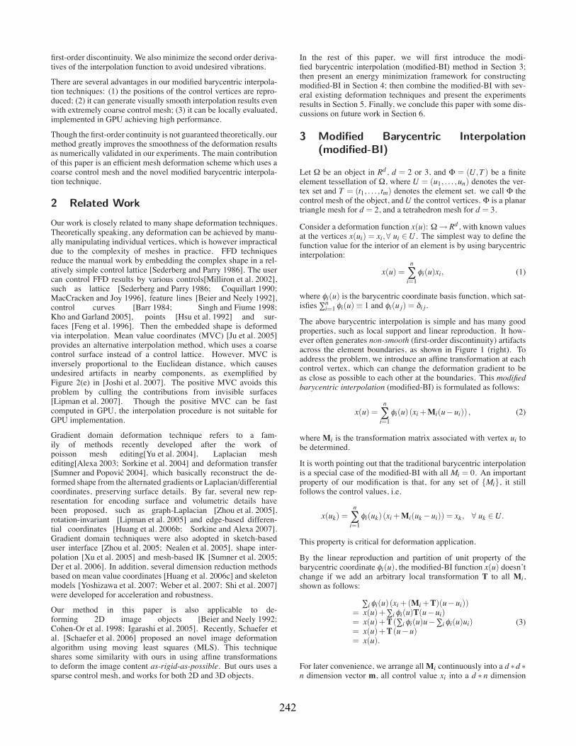
Figure 3: Comparison of deformation results with various userspecified α values in Equation (8).
4.4 Weighting Scheme
We can manipulate the importance of the vibration and discontinu-ity energy by adjusting the weighting coefficients in Equation (8).We first set α = 1 and automatically choose a value for β such thatEvibr(x) and β Edisc(x) are comparable, i.e., their Hessian matriceshave the same Frobenius norm. Then the user is allowed to manu-ally adjust the value of α to balance between fairness and continuityof the interpolation result.
In Figure 3 we use a 2D example to demonstrate the affections ofdifferent α values. As expected, when we increase α , the resultis more like a BI result as shown in Figure 3(b) since BI have thesmallest fairness energy (= 0); when we decrease α , the result be-comes more smooth across the control mesh’s element boundary asshown in Figure 3(c); but vibration occurs when α approaches tozero as shown in Figure 3(d). We empirically found that α = 0.2and α = 0.1 work well respectively for 2D objects and 3D objects.
5 Implementation and Results
We have implemented a deformation system using the modified-BI for interpolation and several existing techniques for manipulat-ing the coarse control mesh. We generate the coarse tetrahedronmeshes for the target objects using an automatic mesh generator –NETGEN (http://www.hpfem.jku.at/netgen/). We extrude the sur-face outward so that the generated tetrahedron mesh fully envelopsthe target object.
To accelerate minimizing the total energy Etotal(x) of the modified-BI, we precomputed a Cholesky factorization for the matrix of theresultant linear system. For the Stanford Bunny object, the pre-computing step (calculating the Hesse matrix about m and x) takesabout less than 1s, the run-time step takes about 4ms for solvingthe linear systems and 17ms for interpolating the fine mesh re-spectively. Taking advantage of the local support property of themodified-BI, we implement interpolation in GPU, which achievesabout 6 ∼ 9 times of acceleration. A detailed performance list issummarized in Table 1.
In Figure 1 and Figure 4 are some deformation results of 3D ob-jects. We embed the 3D object with coarse tetrahedron mesh, andrun physically-based simulation method [Muller and Gross 2004;Huang et al. 2006a] to manipulate the control mesh. The targetobject embedded in the control mesh is deformed by using ourmodified-BI.
Figure 1 is a typical twisting example. We computed the discon-
Bar Dragon 2Pho Bunny Dinosor
Mean5.90 2.64 7.35 9.37 5.97
0.025 0.024 0.084 0.095 0.054236 110 87.5 102 111
1StdDev4.54 52.6 4.46 84.5 40.3
0.029 0.23 0.073 0.46 0.33156 228 61 184 122
Max16.8 584 345 956 436
0.189 4.3 1.55 7.38 3.3588.9 136 222 130 130
1StdDev – Standard Deviation. 2Pho – Phonograph.
Table 2: Numerical results of the discontinuity energy. In each cell,the values from top to down are respectively values of barycentricinterpolation, modified-BI and their ratio.
tinuity energies Edisc(x) (see Equation (5)) for all shared bound-aries on the coarse control mesh. For this twisting example,The Max/Mean/StdDev(Standard Deviation) of the energies forthe barycentric interpolation and modified-BI, and their ratios areshown in the ”Bar” column of Table 2. The energy ratios showedthat the modified-BI reduced the discontinuity down to less than1/150. The other columns in Table 2 for different object and defor-mation poses also demonstrate that our method improves the defor-mation results greatly.
Figure 4: Deformation results. Top: the original 3D model embed-ded in a coarse tetrahedron mesh; Middle: results by modified-BI;Bottom: results by barycentric interpolation, where apparent first-order discontinuity artifacts exist.
Figure 4 also compares the results with those of the traditionalbarycentric interpolation. These comparisons show that modified-BI produces visually smooth warping results, while barycentric in-terpolation produces undesired crease artifacts due to its piecewiselinear property. More deformation results on the Phonograph modelare shown in Figure 5.
In Figure 6 are some deformation results of the Dragon model.For this example, the coarse tetrahedron mesh is manipulatedby regarding the tetrahedron control mesh as a volumetric graphand using the volumetric graph Laplacian [Zhou et al. 2005] rep-resentation. To relax the user from specifying the rotation
244
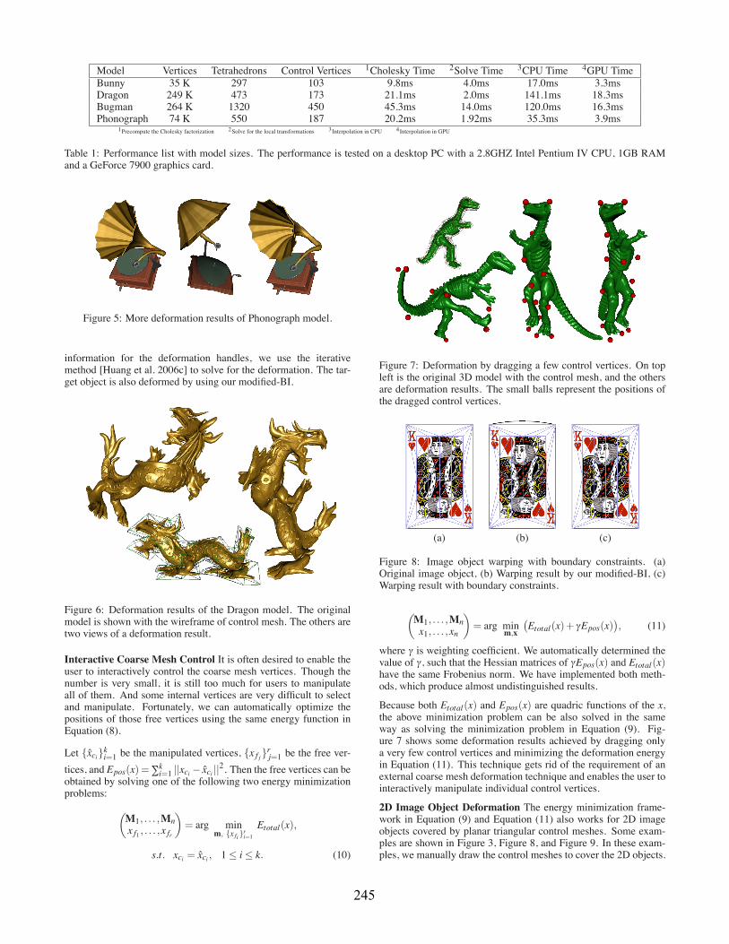
Model Vertices Tetrahedrons Control Vertices 1Cholesky Time 2Solve Time 3CPU Time 4GPU TimeBunny 35 K 297 103 9.8ms 4.0ms 17.0ms 3.3msDragon 249 K 473 173 21.1ms 2.0ms 141.1ms 18.3msBugman 264 K 1320 450 45.3ms 14.0ms 120.0ms 16.3msPhonograph 74 K 550 187 20.2ms 1.92ms 35.3ms 3.9ms
1Precompute the Cholesky factorization 2Solve for the local transformations 3Interpolation in CPU 4Interpolation in GPU
Table 1: Performance list with model sizes. The performance is tested on a desktop PC with a 2.8GHZ Intel Pentium IV CPU, 1GB RAMand a GeForce 7900 graphics card.
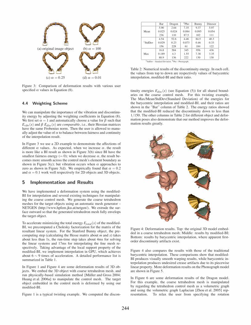
Figure 5: More deformation results of Phonograph model.
information for the deformation handles, we use the iterativemethod [Huang et al. 2006c] to solve for the deformation. The tar-get object is also deformed by using our modified-BI.
Figure 6: Deformation results of the Dragon model. The originalmodel is shown with the wireframe of control mesh. The others aretwo views of a deformation result.
Interactive Coarse Mesh Control It is often desired to enable theuser to interactively control the coarse mesh vertices. Though thenumber is very small, it is still too much for users to manipulateall of them. And some internal vertices are very difficult to selectand manipulate. Fortunately, we can automatically optimize thepositions of those free vertices using the same energy function inEquation (8).
Let {xci}ki=1 be the manipulated vertices, {x f j}r
j=1 be the free ver-
tices, and Epos(x) =∑ki=1 ||xci − xci ||2. Then the free vertices can be
obtained by solving one of the following two energy minimizationproblems:
(M1, . . . ,Mnx f1 , . . . ,x fr
)= arg min
m, {x fi}ri=1
Etotal(x),
s.t. xci = xci , 1 ≤ i ≤ k. (10)
Figure 7: Deformation by dragging a few control vertices. On topleft is the original 3D model with the control mesh, and the othersare deformation results. The small balls represent the positions ofthe dragged control vertices.
(a) (b) (c)
Figure 8: Image object warping with boundary constraints. (a)Original image object, (b) Warping result by our modified-BI, (c)Warping result with boundary constraints.
(M1, . . . ,Mnx1, . . . ,xn
)= arg min
m,x
(Etotal(x)+ γEpos(x)
), (11)
where γ is weighting coefficient. We automatically determined thevalue of γ , such that the Hessian matrices of γEpos(x) and Etotal(x)have the same Frobenius norm. We have implemented both meth-ods, which produce almost undistinguished results.
Because both Etotal(x) and Epos(x) are quadric functions of the x,the above minimization problem can be also solved in the sameway as solving the minimization problem in Equation (9). Fig-ure 7 shows some deformation results achieved by dragging onlya very few control vertices and minimizing the deformation energyin Equation (11). This technique gets rid of the requirement of anexternal coarse mesh deformation technique and enables the user tointeractively manipulate individual control vertices.
2D Image Object Deformation The energy minimization frame-work in Equation (9) and Equation (11) also works for 2D imageobjects covered by planar triangular control meshes. Some exam-ples are shown in Figure 3, Figure 8, and Figure 9. In these exam-ples, we manually draw the control meshes to cover the 2D objects.
245
Figure 9: Examples of 2D image object deformation. On top leftis the original image with coarse control mesh, and the others aredeformation results. The small red balls represent the deformationhandles.
In Figure 8, the user intends to elongate the human face by draggingseveral control points. As shown in Figure 8(b), the straight line ofthe top boundary is bent. Such bending is caused by the local trans-formation for minimizing the gradient discontinuity and vibrations.To void such undesired bending, we constrain the local transforma-tions of the outmost control vertices to be zero when minimizingEtotal(x) in Equation (8). The result of such constrained method isshown in Figure 8(c), where the bending is effectively avoided.
Figure 9 shows several 2D deformation results, obtained by drag-ging only a few (4 ∼ 6) control vertices, and solving the energyminimization problem described in Equation (11).
6 Conclusion and Future Work
We have presented an efficient deformation method based on anovel interpolation technique – modified barycentric interpolation(modified-BI). The experimental results have demonstrated thatmodified-BI is very successful in 2D image and 3D shape defor-mation, Using the modified-BI, extremely coarse mesh can be usedto greatly reduce the simulation/deformation cost.
The major limitation of modified-BI is that it requires solving a lin-ear system for transformation optimization, but this is not criticalsince it is performed on the coarse control mesh. An avenue for fu-ture work is to explore more efficient solvers for the local transfor-mations. Another limitation is that the continuity of the modified-BI is not theoretically proved though numerically validated in ex-periments. In future, we will intensively study the continuity prob-lem of the modified-BI. One possibility is to take advantage ofthe tetrahedron subdivision method[Schaefer et al. 2004]. We willalso explore more deformation methods by taking advantage of themodified-BI technique, and develop more control techniques andsupport more user constraints.
7 Acknowledgments
We would like to thank the reviewers for their valuable com-ments. This work is supported in partial by the 973 Programof China (No.2002CB312100 and No.2006CB303102), NSFC(No.60603078), the Program for New Century Excellent Talents inUniversity of China (No. NCET-06-0516) and the National HighTechnology Research and Development Program of China (No.2007AA01Z336).
References
ALEXA, M. 2003. Differential coordinates for local mesh morph-ing and deformation. The Visual Computer 19, 2, 105–114.
BARR, A. H. 1984. Global and local deformations of solid primi-tives. In SIGGRAPH, 21–30.
BEIER, T., AND NEELY, S. 1992. Feature-based image metamor-phosis. Computer Graphics 26, 2, 35–42.
BOTSCH, M., AND KOBBELT, L. 2004. An intuitive frameworkfor real-time freeform modeling. ACM Trans. Graph. 23, 3, 630–634.
BOTSCH, M., AND KOBBELT, L. 2005. Real-time shape editingusing radial basis functions. Computer Graphics Forum 24, 3,611–621.
COHEN-OR, D., SOLOMOVIC, A., AND LEVIN, D. 1998. Three-dimensional distance field metamorphosis. ACM Trans. Graph.17, 2, 116–141.
COQUILLART, S. 1990. Extended free-form deformation: a sculp-turing tool for 3d geometric modeling. In SIGGRAPH, 187–196.
DER, K. G., SUMNER, R. W., AND POPOVIC, J. 2006. In-verse kinematics for reduced deformable models. In ACM SIG-GRAPH, 1174–1179.
FENG, J., MA, L., AND PENG, Q. 1996. A new free-form defor-mation through the control of parametric surfaces. Computers &Graphics 20, 4, 531–539.
FLOATER, M. S. 2003. Mean value coordinates. Comput. AidedGeom. Des. 20, 1, 19–27.
HSU, W. M., HUGHES, J. F., AND KAUFMAN, H. 1992. Directmanipulation of free-form deformations. In SIGGRAPH, 177–184.
HUANG, J., LIU, X., BAO, H., GUO, B., AND SHUM, H.-Y. 2006.An efficient large deformation method using domain decompo-sition. Computers & Graphics 30, 6, 927–935.
HUANG, J., SHI, X., LIU, X., ZHOU, K., GUO, B., AND BAO,H. 2006. Geometrically based potential energy for simulatingdeformable objects. The Visual Computer 22, 9, 740–748.
IGARASHI, T., MOSCOVICH, T., AND HUGHES, J. F. 2005. As-rigid-as-possible shape manipulation. ACM Trans. Graph. 24, 3,1134–1141.
JOSHI, P., MEYER, M., DEROSE, T., GREEN, B., ANDSANOCKI, T. 2007. Harmonic coordinates for character articu-lation. ACM Trans. Graph. 26, 3, 71.
JU, T., SCHAEFER, S., AND WARREN, J. 2005. Mean value coor-dinates for closed triangular meshes. ACM Trans. Graph. 24, 3,561–566.
KHO, Y., AND GARLAND, M. 2005. Sketching mesh deforma-tions. In Proceedings of the symposium on Interactive 3D graph-ics and games, 147–154.
LIPMAN, Y., SORKINE, O., LEVIN, D., AND COHEN-OR, D.2005. Linear rotation-invariant coordinates for meshes. ACMTrans. Graph. 24, 3, 479–487.
246
LIPMAN, Y., KOPF, J., COHEN-OR, D., AND LEVIN, D. 2007.Gpu-assisted positive mean value coordinates for mesh defor-mations. In Eurographics symposium on Geometry processing,117–123.
MACCRACKEN, R., AND JOY, K. I. 1996. Free-form deformationswith lattices of arbitrary topology. In SIGGRAPH, 181–188.
MILLIRON, T., JENSEN, R. J., BARZEL, R., AND FINKELSTEIN,A. 2002. A framework for geometric warps and deformations.ACM Trans. Graph. 21, 1, 20–51.
MORETON, H. P., AND SEQUIN, C. H. 1992. Functional opti-mization for fair surface design. In SIGGRAPH, 167–176.
MULLER, M., AND GROSS, M. 2004. Interactive virtual materials.In Proceedings of the 2004 conference on Graphics interface,239–246.
NEALEN, A., SORKINE, O., ALEXA, M., AND COHEN-OR, D.2005. A sketch-based interface for detail-preserving mesh edit-ing. In SIGGRAPH ’05: ACM SIGGRAPH 2005 Papers, 1142–1147.
SCHAEFER, S., HAKENBERG, J., AND WARREN, J. 2004. Smoothsubdivision of tetrahedral meshes. In Eurographics/ACM SIG-GRAPH symposium on Geometry processing, 147–154.
SCHAEFER, S., MCPHAIL, T., AND WARREN, J. 2006. Imagedeformation using moving least squares. ACM Trans. Graph.25, 3, 533–540.
SEDERBERG, T. W., AND PARRY, S. R. 1986. Free-form deforma-tion of solid geometric models. In SIGGRAPH ’86, ACM Press,151–160.
SHI, X., ZHOU, K., TONG, Y., DESBRUN, M., BAO, H., ANDGUO, B. 2007. Mesh puppetry: cascading optimization of meshdeformation with inverse kinematics. ACM Trans. Graph. 26, 3,81.
SINGH, K., AND FIUME, E. 1998. Wires: a geometric deformationtechnique. In SIGGRAPH, 405–414.
SORKINE, O., AND ALEXA, M. 2007. As-rigid-as-possiblesurface modeling. In Proceedings of Eurographics/ACM SIG-GRAPH Symposium on Geometry Processing, 109–116.
SORKINE, O., LIPMAN, Y., COHEN-OR, D., ALEXA, M.,ROSSL, C., AND SEIDEL, H.-P. 2004. Laplacian surface edit-ing. In Proceedings of the Eurographics symposium on Geome-try processing, 179–188.
SUMNER, R. W., AND POPOVIC, J. 2004. Deformation transferfor triangle meshes. In SIGGRAPH ’04: ACM SIGGRAPH 2004Papers, 399–405.
SUMNER, R. W., ZWICKER, M., GOTSMAN, C., AND POPOVIC,J. 2005. Mesh-based inverse kinematics. In ACM SIGGRAPH,488–495.
WEBER, O., SORKINE, O., LIPMAN, Y., AND GOTSMAN, C.2007. Context-aware skeletal shape deformation. ComputerGraphics Forum (Proceedings of Eurographics) 26, 3.
WELCH, W., AND WITKIN, A. 1992. Variational surface model-ing. In SIGGRAPH, 157–166.
XU, D., ZHANG, H., WANG, Q., AND BAO, H. 2005. Poissonshape interpolation. In SPM ’05, ACM Press, 267–274.
YOSHIZAWA, S., BELYAEV, A. G., AND SEIDEL, H.-P. 2007.Skeleton-based variational mesh deformations. ComputerGraphics Forum, 255–264.
YU, Y., ZHOU, K., XU, D., SHI, X., BAO, H., GUO, B., ANDSHUM, H.-Y. 2004. Mesh editing with poisson-based gradientfield manipulation. ACM Trans. Graph. 23, 3, 644–651.
ZAYER, R., ROSSL, C., KARNI, Z., AND SEIDEL, H.-P. 2005.Harmonic guidance for surface deformation. Computer Graph-ics Forum, Proceedings of Eurographics 2005 24, 3, 601–609.
ZHOU, K., HUANG, J., SNYDER, J., LIU, X., BAO, H., GUO, B.,AND SHUM, H.-Y. 2005. Large mesh deformation using thevolumetric graph laplacian. ACM Trans. Graph. 24, 3, 496–503.