Eﬃcientnumericalcomputationofdirectexchangeareasinthermal … · ·...

This document contains a post-print version of the paper

Efficient numerical computation of direct exchange areas in thermalradiation analysis

authored by M. Feischl, T. Führer, M. Niederer, S. Strommer, A. Steinboeck, and D. Praetorius

and published in Numerical Heat Transfer, Part B: Fundamentals.

The content of this post-print version is identical to the published paper but without the publisher’s final layout orcopy editing. Please, scroll down for the article.

Cite this article as:M. Feischl, T. Führer, M. Niederer, S. Strommer, A. Steinboeck, and D. Praetorius, “Efficient numerical computationof direct exchange areas in thermal radiation analysis”, Numerical heat transfer, part b: Fundamentals, vol. 69, no. 6,pp. 511–533, 2016. doi: 10.1080/10407790.2016.1173469

BibTex entry:@ARTICLE{acinpaper,AUTHOR = {Feischl, M. and F\"uhrer, T. and Niederer, M. and

Strommer, S. and Steinboeck, A. and Praetorius, D.},TITLE = {Efficient numerical computation of direct exchange

areas in thermal radiation analysis},JOURNAL = {Numerical Heat Transfer, Part B: Fundamentals},YEAR = {2016},volume = {69},number = {6},pages = {511--533},doi = {10.1080/10407790.2016.1173469},url = {http://www.tandfonline.com/doi/full/10.1080/10407790.2016.1173469}

}

Link to original paper:http://dx.doi.org/10.1080/10407790.2016.1173469http://www.tandfonline.com/doi/full/10.1080/10407790.2016.1173469

Read more ACIN papers or get this document:http://www.acin.tuwien.ac.at/literature

Contact:Automation and Control Institute (ACIN) Internet: www.acin.tuwien.ac.atVienna University of Technology E-mail: [email protected] 27-29/E376 Phone: +43 1 58801 376011040 Vienna, Austria Fax: +43 1 58801 37699

http://dx.doi.org/10.1080/10407790.2016.1173469

http://dx.doi.org/10.1080/10407790.2016.1173469

http://www.tandfonline.com/doi/full/10.1080/10407790.2016.1173469

http://www.acin.tuwien.ac.at/literature

www.acin.tuwien.ac.at

mailto:[email protected]

Copyright notice:This is the authors’ version of a work that was accepted for publication in Numerical Heat Transfer, Part B: Fundamentals. Changesresulting from the publishing process, such as peer review, editing, corrections, structural formatting, and other quality control mechanismsmay not be reflected in this document. Changes may have been made to this work since it was submitted for publication. A definitiveversion was subsequently published in M. Feischl, T. Führer, M. Niederer, S. Strommer, A. Steinboeck, and D. Praetorius, “Efficientnumerical computation of direct exchange areas in thermal radiation analysis”, Numerical heat transfer, part b: Fundamentals, vol. 69, no.6, pp. 511–533, 2016. doi: 10.1080/10407790.2016.1173469

http://dx.doi.org/10.1080/10407790.2016.1173469

Numerical Heat Transfer, Part B: Fundamentals

Vol. 69, No. 6, October 2016, 1–34

Contributed Paper

EFFICIENT NUMERICAL COMPUTATION OF DIRECT

EXCHANGE AREAS IN THERMAL RADIATION ANALYSIS

Abbreviated title: EFFICIENT COMPUTATION OF DIRECT EXCHANGE AREAS

M. Feischla, T. Fuhrera, M. Niedererb, S. Strommerb, A. Steinboeckb,∗, and D. Praetoriusa

aInstitute of Analysis and Scientific Computing, Vienna University of Technology,

Wiedner Hauptstraße 8, 1040 Vienna, Austria

bAutomation and Control Institute, Vienna University of Technology,

Gußhausstraße 27–29, 1040 Vienna, Austria

(Received 7 September 2015; final version received 11 November 2015)

Abstract: The analysis of thermal radiation in multi-surface enclosures typically involves

multiple integrals with four, five, or six variables. Major difficulties for the numerical evalu-

ation of these integrals are non-convex geometries and singular integral kernels. This paper

presents hierarchical visibility concepts and coordinate transformations which eliminate these

difficulties. In the transformed form, standard quadrature techniques are applied and accurate

results are achieved with moderate numerical effort. In benchmark example problems, the

effectiveness and accuracy of the method are validated. A simulation model of an industrial

furnace demonstrates the applicability of the method for large-scale problems.

NOMENCLATURE

Bα bounding box

b radiosity, W/m2

C(α) function for computing the visibility

D integration domain

d side length, distance, m

f continuous function or part of the kernel k, m4

g part of the integral kernel k, 1/m2

H heat flux density absorbed by a volume zone, W/m2

∗Corresponding author. Email: [email protected]

1

Post-print version of the article: M. Feischl, T. Führer, M. Niederer, S. Strommer, A. Steinboeck, and D. Praetorius, “Efficient numericalcomputation of direct exchange areas in thermal radiation analysis”, Numerical heat transfer, part b: Fundamentals, vol. 69, no. 6, pp. 511–533, 2016. doi: 10.1080/10407790.2016.1173469The content of this post-print version is identical to the published paper but without the publisher’s final layout or copy editing.

http://dx.doi.org/10.1080/10407790.2016.1173469

h irradiance, W/m2

I total intensity, W/(m2sr)

K absorption coefficient, 1/m

k integral kernel, 1/m4

M order of quadrature

NS number of surface zones

NV number of volume zones

Q net heat flow into volume zone, W

q net heat flow into surface zone, W

r distance coordinate along a ray, m

rj , rij geometrical length of a ray, m

rij optical length of a ray

Sα set of barycenters of surfaces zones

S(α) functions for generating a hierarchy of bounding boxes

S surface zone, surface area, m2

s evaluation point of Gaussian quadrature

sisj surface-surface direct exchange area, m2

sivj surface-volume direct exchange area, m2

T gas temperature, K

t surface temperature, K

V volume zone, volume, m3

Vref reference volume zone

visj volume-surface direct exchange area, m2

vivj volume-volume direct exchange area, m2

W integration domain

w weight of Gaussian quadrature

~x coordinates in volume zone, m

α tuple

~α, ~β normalized coordinates in reference volume zone

~γ relative coordinates

ε emissivity

θ incident or emergent angle, rad

Λ coordinate transformation

σ Stefan-Boltzmann constant, W/(m2K4)

Φ function for a transformation of integration domains

Subscripts

2


http://dx.doi.org/10.1080/10407790.2016.1173469

i, j index of zone or index value

k, n index value

1. INTRODUCTION

Heat transfer by gray thermal radiation in enclosures formed by diffuse surfaces and filled

with participating gas can be efficiently analyzed by means of the zone method [1]. Instead

of a rigorous solution of the multiple integrals that emerge from the direct application of

the radiative transfer equation [2, 3], the zone method uses a spatial discretization of the

radiation geometry to obtain a finite-dimensional linear relation between the radiative

heat flows and the fourth powers of the temperatures. The discretization is found by di-

viding the calculation domain into isothermal surface and volume sections. The approach

may be considered as a numerical quadrature method that facilitates a direct geometric

interpretation.

The zone method, which was originally suggested by Hottel and coworkers [1, 4], is

described in detail in [2, 3]. Section 1.1 of this paper provides a concise overview of

this method. Reviews of various other modeling methods for radiative heat transfer are

reported in [5, 6, 7, 8, 9, 10, 11].

According to [8], the zone method is one of the fastest approaches for analyzing thermal

radiation if the exchange areas are known. However, the calculation of direct exchange

areas is still a time-consuming and thus limiting factor of the zone method. In fact, it

involves integrals with four, five, or six variables [2, 3]. Currently, there is no perspective

to compute direct exchange areas in real time. Despite growing computer power and the

advent of multi-core systems and parallel computing, the computation of direct exchange

areas for general three-dimensional problems with complex geometries is still not feasi-

ble within reasonable times. This conclusion may also be drawn from the literature in

this field, which is briefly reviewed in Section 1.2. The lack of an efficient method for

calculating direct exchange areas is the principal impetus for this work.

The paper is organized as follows: Section 2 demonstrates that the multiple integrals

associated with direct exchange areas should not be solved by direct application of numer-

ical quadrature techniques due to singularity problems. Therefore, we explore in Section

3 how coordinate and geometric transformations can avoid these singularities. In Section

4, we validated the effectiveness and accuracy of the method based on benchmark exam-

ple problems. In a case study, we use the approach in a simulation model of an industrial

furnace and compare the simulation results with measurements from the real plant. This

demonstrates the applicability of the method to large-scale problems.

3


http://dx.doi.org/10.1080/10407790.2016.1173469

1.1. Zone Method

Consider a volume that is filled with participating gas. In this volume, let the straight

path of a single ray of thermal radiation be parameterized by the distance coordinate

r. The total intensity of the ray at some point r is I(r). From the radiative transfer

equation [2, 3], it is known that the total intensity of the ray is attenuated according to

I(rj) = I(ri)e−rij (1)

as it travels from r = ri to r = rj through the participating gas. The dimensionless

quantity

rij =

∫ rj

ri

K(r)dr (2)

with the absorption coefficient K(r) is also known as optical thickness of the path from

ri to rj . In a gaseous medium where K is constant, K−1 is the mean free path of a

photon until it is absorbed. In Eq. (1), we have not considered that the total intensity

may also increase because of radiative emission of the gas itself. This effect is captured

by the term

K(r)σ

πT 4dV , (3)

which is the total heat flux emitted by an infinitesimal volume element dV per unit solid

angle. T is the local gas temperature and σ is the Stefan-Boltzmann constant. The term

σT 4/π represents the total intensity of black bodies.

dS, t, ε

θ

Figure 1. Emergent angle of an emitting surface.

An infinitesimal section dS of a solid, gray, diffuse surface with the temperature t emits

the directional total heat flux

εσ

πt4 cos(θ)dS (4)

per unit solid angle. The radiative heat flux depends on the emergent angle θ ∈ [0, π/2]

(cf. Fig. 1) insofar as it is proportional to the projected area cos(θ)dS of the emitter.

Moreover, it is proportional to the emissivity ε ∈ [0, 1], which is a surface property.

4


http://dx.doi.org/10.1080/10407790.2016.1173469

S1 S2

Sj , tj

Sn

qj

Vi,Ti

V1

V2VN

Qi

Figure 2. Opaque enclosure filled by participating gas.

dSi

dSj

rijθiθj

(a) Relation between two sur-faces.

dSi

rijθi

dVj

(b) Relation between surfaceand volume.

rij

dVj

dVi

(c) Relation between two vol-umes.

Figure 3. Geometric relation between two infinitesimal zone sections.

Sj

hjSj bjSj

qj

(a) Net radiative heat flow into a sur-face zone.

Vj

Hj4KjVj σT 4j 4KjVj

Qj

(b) Net radiative heat flow into a vol-ume zone.

Figure 4. Net radiative heat flows into zones.

We are interested in the heat flows inside an opaque enclosure filled by a participating

gaseous medium. The situation is outlined in Fig. 2. For the zone method, the enclosing

surface and the internal volume are partitioned into NS isothermal surface zones and

NV isothermal volume zones, respectively. Then, linear relations between radiative flows

diffusely emitted by a zone i (emitter) and the portion of it that is directly absorbed or

reflected by the zone j (receiver) can be found. The factors defining these linear relations

are called direct exchange areas. They can be computed by integration over all possible

rays of thermal radiation traveling from the emitter i through the participating medium

directly to the receiver j. Possible rays of thermal radiation are shown in Fig. 3. The

geometric path length of these rays is rij, their optical thickness is rij , and according to

(1) their intensity is reduced by the factor e−rij (transmittance).

Throughout the following analysis, we assume that the temperature and the emissivity

or the absorption coefficient are uniform within the respective zone. For a surface zone

j, we thus have t = tj and ε = εj . For a volume zone j, we have T = Tj and K = Kj.

Assume that hjSj is the total radiative heat flow that is incident onto the surface Sj

(hj is known as irradiance). The portion εjhjSj of hjSj is absorbed by the opaque surface

5


http://dx.doi.org/10.1080/10407790.2016.1173469

and the remaining part (1− εj)hjSj is reflected. Let the surface have the temperature tj

so that the emitted radiative heat flow is εjσt4jSj. Thus,

bjSj = ((1 − εj)hj + εjσt4j)Sj (5)

is the total radiative heat flow that departs from the surface Sj (bj is known as radiosity).

As indicated in Fig. 4(a), this yields the net radiative heat flow into the surface

qj = (hj − bj)Sj = εj(hj − σt4j)Sj . (6)

For volume zones, the situation is somewhat simpler because they do not reflect ra-

diation. Assume that 4KjVjHj is the radiative heat flow absorbed by a volume Vj .

Integrating Eq. (3) over all possible spatial directions (full solid angle, 4πsr) yields that

the volume emits the radiative heat flow σT 4j 4KjVj if Tj is the uniform temperature of

the gas in the volume. Consequently, the net radiative heat flow into the volume Vj (cf.

Fig. 4(b)) is

Qj = (Hj − σT 4j )4KjVj. (7)

The remaining unknowns hj and Hj can be computed from a radiation balance, i. e., by

summing up the heat flows departing from surface and volume zones. Consider first the

interacting surface zones Si and Sj. The portion of Sjhj that comes directly from Si is

found by integrating over all possible rays of thermal radiation between the two surfaces,

i. e.,

bi

∫

Si

∫

Sj

cos(θi) cos(θj)e−rij

πr2ijdSjdSi

︸︷︷︸=: sisj

, (8)

where sisj ∈ [0,min(Si, Sj)] is called surface-surface direct exchange area. Eq. (8) can be

deduced by consideration of Fig. 3(a), Eq. (1), Eq. (4), and the fact that dSj occupies

the solid angle cos(θj)dSj/r2ij in the field of view of dSi.

Next, consider a volume Vi and a surface Sj. The portion of Sjhj that comes directly

from Vi is found by integrating over all possible rays of thermal radiation between the

6


http://dx.doi.org/10.1080/10407790.2016.1173469

two zones, i. e.,

σT 4i

∫

Vi

∫

Sj

cos(θj)Kie−rij

πr2ijdSjdVi

︸︷︷︸=: visj

, (9)

where visj ∈ [0,min(4KiVi, Sj)] is called volume-surface direct exchange area. Eq. (9)

can be deduced by consideration of Fig. 3(b), Eq. (1), Eq. (3), and the fact that dSj

occupies the solid angle cos(θj)dSj/r2ij in the field of view of dVi.

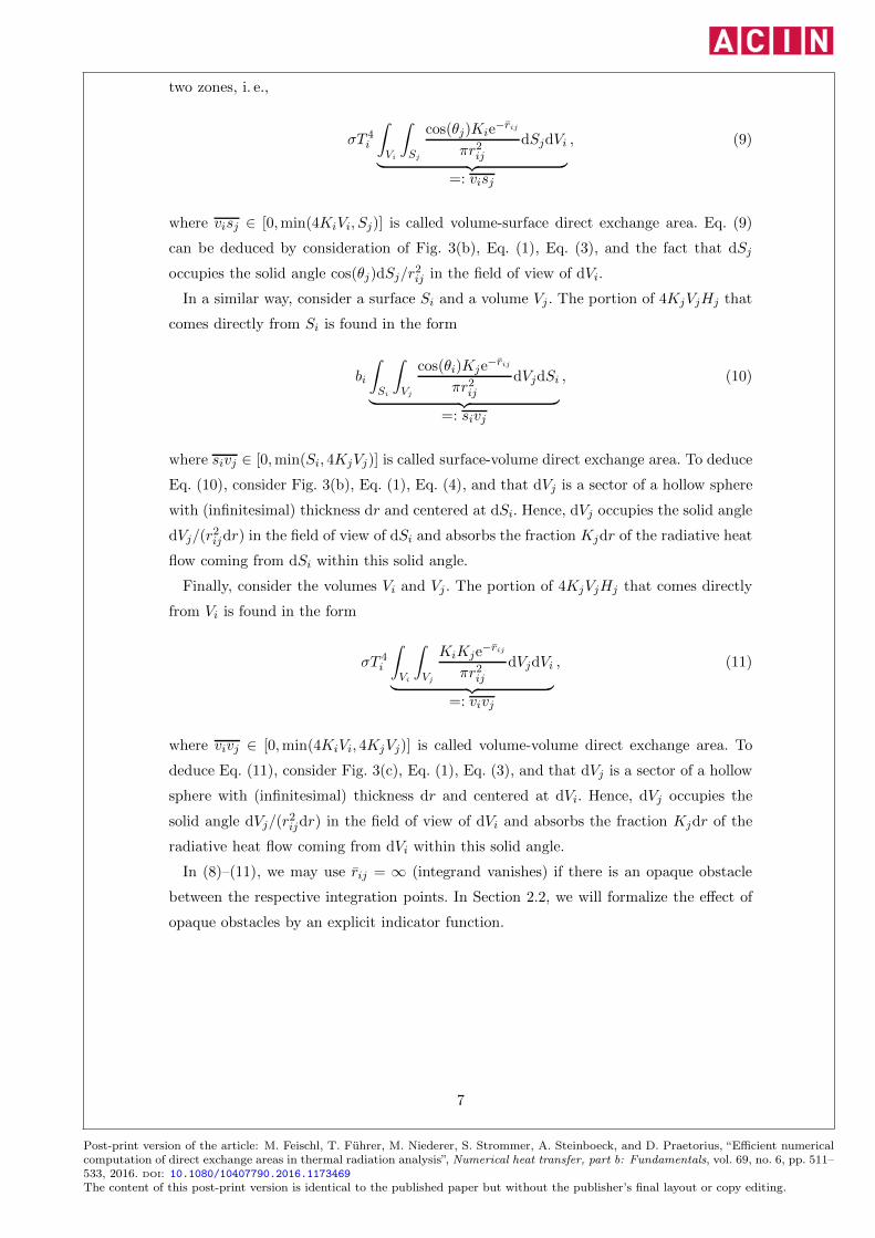
In a similar way, consider a surface Si and a volume Vj . The portion of 4KjVjHj that

comes directly from Si is found in the form

bi

∫

Si

∫

Vj

cos(θi)Kje−rij

πr2ijdVjdSi

︸︷︷︸=: sivj

, (10)

where sivj ∈ [0,min(Si, 4KjVj)] is called surface-volume direct exchange area. To deduce

Eq. (10), consider Fig. 3(b), Eq. (1), Eq. (4), and that dVj is a sector of a hollow sphere

with (infinitesimal) thickness dr and centered at dSi. Hence, dVj occupies the solid angle

dVj/(r2ijdr) in the field of view of dSi and absorbs the fraction Kjdr of the radiative heat

flow coming from dSi within this solid angle.

Finally, consider the volumes Vi and Vj . The portion of 4KjVjHj that comes directly

from Vi is found in the form

σT 4i

∫

Vi

∫

Vj

KiKje−rij

πr2ijdVjdVi

︸︷︷︸=: vivj

, (11)

where vivj ∈ [0,min(4KiVi, 4KjVj)] is called volume-volume direct exchange area. To

deduce Eq. (11), consider Fig. 3(c), Eq. (1), Eq. (3), and that dVj is a sector of a hollow

sphere with (infinitesimal) thickness dr and centered at dVi. Hence, dVj occupies the

solid angle dVj/(r2ijdr) in the field of view of dVi and absorbs the fraction Kjdr of the

radiative heat flow coming from dVi within this solid angle.

In (8)–(11), we may use rij = ∞ (integrand vanishes) if there is an opaque obstacle

between the respective integration points. In Section 2.2, we will formalize the effect of

opaque obstacles by an explicit indicator function.

7


http://dx.doi.org/10.1080/10407790.2016.1173469

Based on Eqs. (5) and (8)–(11), we can compute the total radiative heat flow

Sjhj =

NS∑

i=1

((1− εi)hi + εiσt4i )sisj +

NV∑

i=1

σT 4i visj (12)

that is incident onto the surface Sj and the total radiative heat flow

4KjVjHj =

NS∑

i=1

((1− εi)hi + εiσt4i )sivj +

NV∑

i=1

σT 4i vivj (13)

that is absorbed by the volume zone Vj. Elimination of all variables hj andHj in Eqs. (6),

(7), (12), and (13) yields the desired linear relations between the fourth powers of zone

temperatures (t4j and T 4j ) and the net heat flows (qj and Qj) associated with thermal

radiation. This concludes the theoretical description of the zone method.

The largest part of the computational effort associated with the zone method is usually

caused by the multiple integrals for calculating the direct exchange areas in Eqs. (8)–(11).

This calculation requires just knowledge of the geometry and the factors Kj. Hence, it

is often done before the evaluation of qj and Qj. If neither the geometry nor the factors

Kj change, there is no need for recalculating direct exchange areas.

Direct exchange areas have the unit of area, even if i or j or both are volume zones.

The formulae in Eqs. (8)–(11) are also applicable for the case i = j. Moreover, they

satisfy the reciprocity relations

sisj = sjsi (14a)

visj = sjvi (14b)

vivj = vjvi (14c)

and the summation rules

Sj =

NS∑

i=1

sisj +

NV∑

i=1

visj (15a)

4KjVj =

NS∑

i=1

sivj +

NV∑

i=1

vivj (15b)

(cf. [2, 3, 10]). These relations can be helpful for validating numerical results of direct

exchange areas or for reducing the workload when computing them. When solving the

multiple integrals in Eqs. (8)–(11), a considerable difficulty is the singularity associated

8


http://dx.doi.org/10.1080/10407790.2016.1173469

with rij → 0. This will be further analyzed in Section 2.

1.2. Existing Approaches for Explicit Calculation of Direct Exchange

Areas

Numerical values for direct exchange areas in rectangular geometries are given in the

form of charts in [12]. Moreover, curve fitting techniques are applied to obtain exponential

functions that approximate the given numerical results [10].

In Cartesian coordinates, the length rij of a ray ~rij = ~xj − ~xi emitted from ~xi to ~xj is

computed by

rij := |~xi − ~xj | :=√

(xi,1 − xj,1)2 + (xi,2 − xj,2)2 + (xi,3 − xj,3)2 (16)

and depends only on the differences xi,1−xj,1, xi,2−xj,2, and xi,3−xj,3. For planar sur-

faces, cos(θi) and cos(θj) also depend only on these differences. If Ki = Kj = K, these

facts can be utilized for reducing the multiple integrals in Eqs. (8)–(11) to integrals with

lower dimensions. This reduced integration scheme was originally proposed by Errku [13].

As demonstrated in [14] for a system with cylindrical coordinates, the scheme safes more

than 80% of the CPU time needed for conventional numerical quadrature. Moreover,

it reduces the severity of most singularities which occur if two zones are adjacent or

overlapping (i = j). In fact, the method described in [14] transfers the singularities to

the boundary of the integration domain but does not remove them. A similar reduced

integration method for direct exchange areas of a cylindrical enclosure is described in

[15]. The methods described in [13, 14, 15] do not consider the mutual visibility between

integration points, i.e., it is not checked whether an opaque obstacle separates the in-

tegration points. The methods are thus only applicable to convex geometries. A mixed

approach is reported in [16], where direct exchange areas of adjacent or overlapping zones

are calculated by means of the finite volume method [17] to circumvent the problem of

singularities. All other direct exchange areas are approximately computed by a midpoint

integration scheme [3]. In this case, the integrands in Eqs. (8)–(11) are only evaluated

at the barycenters of the zones. The accuracy of the method is improved, if the zones

have small optical thicknesses and large optical distances. In [18], the spatial discretiza-

tion is refined by further division of zones and application of the midpoint integration

scheme to the refined grid. To circumvent problems with singularities at overlapping

zones, vanishing center-to-center distances are either replaced by a semi-empirical posi-

tive approximation or the respective direct exchange area is set to zero.

Another reduced integration scheme for direct exchange areas is proposed in [19]. In-

9


http://dx.doi.org/10.1080/10407790.2016.1173469

tegrals over a volume zone Vi are replaced by two-dimensional integrals over the bound-

aries surrounding the volume zone. In fact, only those sections of the boundary of Vi that

are directly visible to the corresponding zone (Sj or Vj) enter the integral. Therefore,

Eqs. (9)–(11) for surface-volume and volume-volume direct exchange areas are simplified

to integrals with only four variables. In [19], the absorbance factor 1− e−Kri, where K is

constant and ri is the geometric length of the ray inside the volume Vi, is multiplied to

the integrand to capture that the fraction e−Kri of the total intensity of the respective

ray passes through the volume (cf. Eq. (1)). A similar approach is presented in [20], but

there the surface integrals that replace the volume integrals over Vi, are evaluated on the

whole boundary of Vi. It is not clear, how the problem of singularities occurring in the

direct exchange areas of adjacent or overlapping zones is tackled in [19] and [20].

A volume zone Vi entails a singular integral kernel when evaluating vivi. Similar prob-

lems occur in the evaluation of the other direct exchange areas defined in Eqs. (8)–(11).

The problem of singularities is usually avoided in the literature by introducing approx-

imations of the respective direct exchange areas. A drawback of this approach is the

possible accumulation of unknown approximation errors and the prevention of a rig-

orous mathematical analysis. The approach may, for instance, cause a violation of the

summation rules Eq. (15) (cf. [14]).

1.3. Avoiding Singular Integral Kernels in the Calculation of Direct

Exchange Areas

In this work, we resolve the problem of singular kernels by applying certain coordinate

transformations which lead to smooth integral kernels that can be evaluated by standard

Gaussian quadrature. Due to strong similarities between the singular kernels in Eqs. (8)–

(11) to those arising in boundary element methods, we adapt the methods proposed in

[21]. The basic ideas are the following: Since the singularity is present at the points which

satisfy ~xi = ~xj, we split the integration domain around these singular points into several

subdomains. After changing the order of integration in these subdomains, the application

of appropriate Duffy transformations removes the singularities, i.e., the resulting integral

kernel is smooth. Intuitively, this is achieved by stretching the points (lines) on which the

singularity is present, to lines (faces). Hence, we conceptually distribute the singularity

on a larger domain and thus remove it. According to the Fubini theorem, this approach

results in multiple 1D line integrals which are approximated by Gaussian quadrature.

Due to the benign numerical properties of the transformed integral kernels, it suffices to

use only a small number of quadrature points. Hence, it requires only low computational

effort to achieve highly accurate results.

10


http://dx.doi.org/10.1080/10407790.2016.1173469

The advantages of the proposed method are manifold: It allows quite general integral

kernels, which can be used, e.g., in the case of non-homogeneous gas-distributions or

in the case of opaque (surfaces) obstacles within the volume zone. The approach gives

reliable results for direct exchange areas in the case of adjacent zones (surface-surface

sisj, volume-surface visj, and volume-volume vivj with i 6= j) and even in the case of self-

interacting zones (surface-surface sisi and volume-volume vivi). Moreover, the method

allows for a thorough mathematical analysis which guarantees exponential accuracy of

the results. For the ease of presentation, we consider axis-parallel volume and surface

zones only. However, the principal ideas transfer to more complex situations.

2. DESCRIPTION OF THE PROBLEM AND SINGULARITIES

To demonstrate the difficulties associated with singular integral kernels, we consider the

volume-volume direct exchange areas from Eq. (11), which can be written as

vivj =

∫

Vi

∫

Vj

k(~xi, ~xj) dVi dVj (17)

where ~xi ∈ Vi and ~xj ∈ Vj are the integration variables and the integrand is

k(~xi, ~xj) :=1

|~xj − ~xi|2KiKj

e−rij

π, (18)

see Eq. (16) for the definition of |~xj − ~xi|. Note that the integrand is smooth for all

~xi 6= ~xj and exhibits singularities for ~xi = ~xj. The latter requires that Vi and Vj overlap

or touch each other. Despite these singularities, the inner integral in Eq. (17) exists as

a proper integral because the integration domain Vj is 3-dimensional but the integrand

k(·, ·) is only singular of order 2. In particular, the Fubini theorem applies and allows to

interchange the order of integration in Eq. (17).

In numerical computations, the possible singularities at ~xi = ~xj impair the accuracy of

quadrature formulas like Gaussian quadrature (cf. Eq. (19)) or may even prohibit their

use. In Section 4.1, we present a numerical example which demonstrates that Gaussian

quadrature may lead to unreliable results for tractable quadrature orders.

11


http://dx.doi.org/10.1080/10407790.2016.1173469

2.1. Geometry

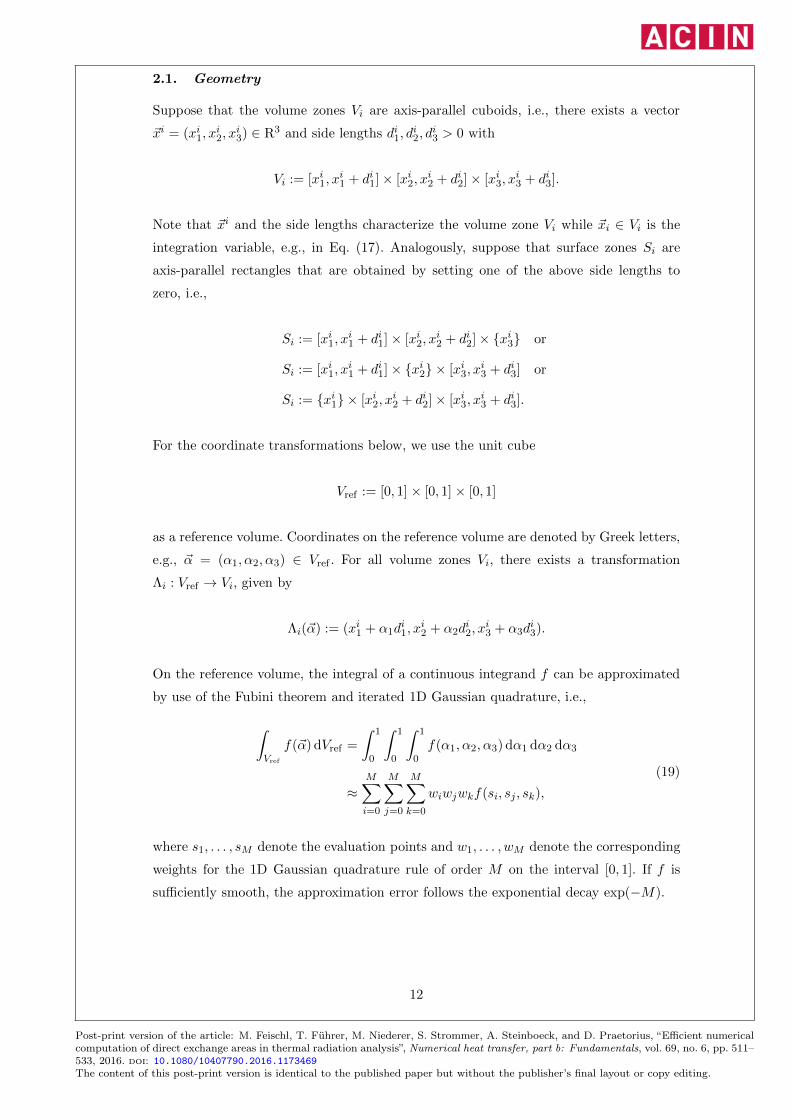
Suppose that the volume zones Vi are axis-parallel cuboids, i.e., there exists a vector

~xi = (xi1, xi2, x

i3) ∈ R3 and side lengths di1, d

i2, d

i3 > 0 with

Vi := [xi1, xi1 + di1]× [xi2, x

i2 + di2]× [xi3, x

i3 + di3].

Note that ~xi and the side lengths characterize the volume zone Vi while ~xi ∈ Vi is the

integration variable, e.g., in Eq. (17). Analogously, suppose that surface zones Si are

axis-parallel rectangles that are obtained by setting one of the above side lengths to

zero, i.e.,

Si := [xi1, xi1 + di1]× [xi2, x

i2 + di2]× {xi3} or

Si := [xi1, xi1 + di1]× {xi2} × [xi3, x

i3 + di3] or

Si := {xi1} × [xi2, xi2 + di2]× [xi3, x

i3 + di3].

For the coordinate transformations below, we use the unit cube

Vref := [0, 1] × [0, 1] × [0, 1]

as a reference volume. Coordinates on the reference volume are denoted by Greek letters,

e.g., ~α = (α1, α2, α3) ∈ Vref . For all volume zones Vi, there exists a transformation

Λi : Vref → Vi, given by

Λi(~α) := (xi1 + α1di1, x

i2 + α2d

i2, x

i3 + α3d

i3).

On the reference volume, the integral of a continuous integrand f can be approximated

by use of the Fubini theorem and iterated 1D Gaussian quadrature, i.e.,

∫

Vref

f(~α) dVref =

∫ 1

0

∫ 1

0

∫ 1

0f(α1, α2, α3) dα1 dα2 dα3

≈M∑

i=0

M∑

j=0

M∑

k=0

wiwjwkf(si, sj, sk),

(19)

where s1, . . . , sM denote the evaluation points and w1, . . . , wM denote the corresponding

weights for the 1D Gaussian quadrature rule of order M on the interval [0, 1]. If f is

sufficiently smooth, the approximation error follows the exponential decay exp(−M).

12


http://dx.doi.org/10.1080/10407790.2016.1173469

2.2. Visibility

In more complex geometries (enclosures), a ray emitted at the point ~xi ∈ Vi and sent

along the direction ~rij = ~xj − ~xi with ~xj ∈ Vj might hit an opaque obstacle before it

arrives at ~xj. Hence, this ray does not contribute to the direct exchange area computed

in Eq. (17). To capture this effect, we extend the kernel k(~xi, ~xj) from Eq. (18) by an

indicator function vis(~xi, ~xj) ∈ {0, 1} to get

k(~xi, ~xj) :=1

|~xj − ~xi|2KiKj

e−rij

πvis(~xi, ~xj). (20)

The indicator function satisfies vis(~xi, ~xj) = 1 if there is no obstacle between ~xi ∈ Vi and

~xj ∈ Vj and vis(~xi, ~xj) = 0 otherwise. At first glance, the evaluation of vis(~xi, ~xj) can

be a challenge in the implementation of complex geometries. However, note that opaque

obstacles are represented by surface zones Sk.

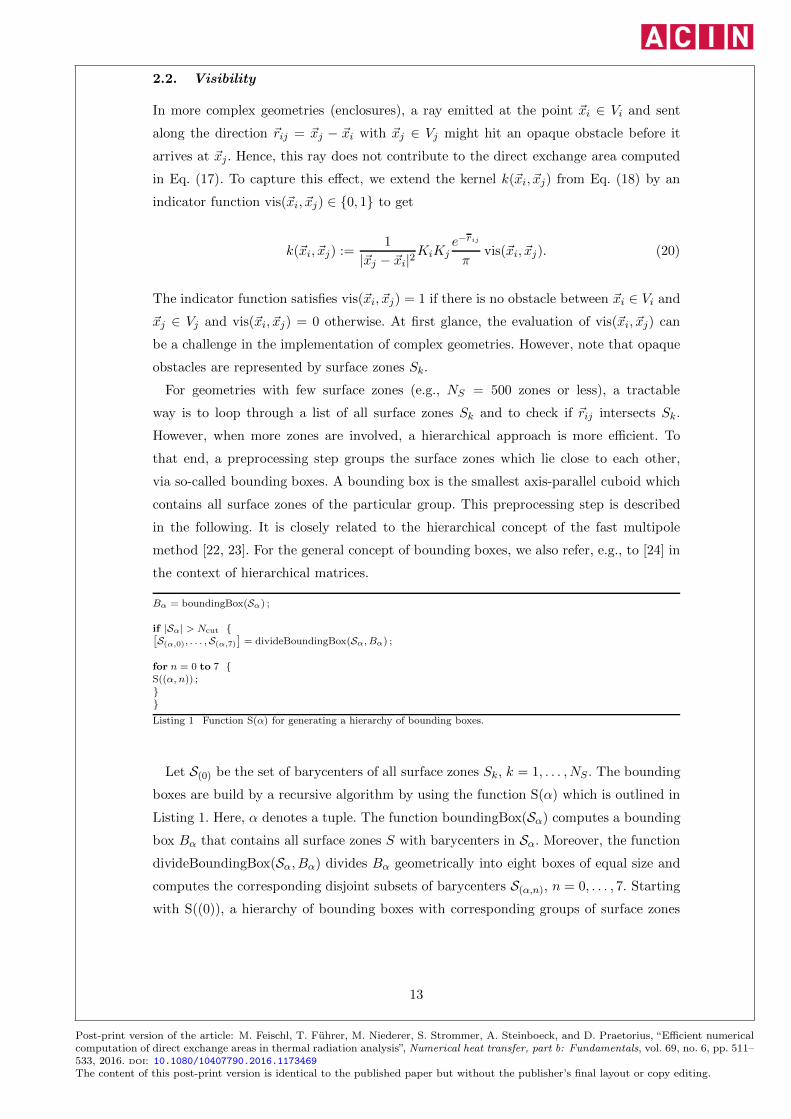
For geometries with few surface zones (e.g., NS = 500 zones or less), a tractable

way is to loop through a list of all surface zones Sk and to check if ~rij intersects Sk.

However, when more zones are involved, a hierarchical approach is more efficient. To

that end, a preprocessing step groups the surface zones which lie close to each other,

via so-called bounding boxes. A bounding box is the smallest axis-parallel cuboid which

contains all surface zones of the particular group. This preprocessing step is described

in the following. It is closely related to the hierarchical concept of the fast multipole

method [22, 23]. For the general concept of bounding boxes, we also refer, e.g., to [24] in

the context of hierarchical matrices.

Bα = boundingBox(Sα) ;

if |Sα| > Ncut {[S(α,0), . . . ,S(α,7)

]= divideBoundingBox(Sα, Bα) ;

for n = 0 to 7 {S((α, n)) ;}}Listing 1 Function S(α) for generating a hierarchy of bounding boxes.

Let S(0) be the set of barycenters of all surface zones Sk, k = 1, . . . , NS . The bounding

boxes are build by a recursive algorithm by using the function S(α) which is outlined in

Listing 1. Here, α denotes a tuple. The function boundingBox(Sα) computes a bounding

box Bα that contains all surface zones S with barycenters in Sα. Moreover, the function

divideBoundingBox(Sα, Bα) divides Bα geometrically into eight boxes of equal size and

computes the corresponding disjoint subsets of barycenters S(α,n), n = 0, . . . , 7. Starting

with S((0)), a hierarchy of bounding boxes with corresponding groups of surface zones

13


http://dx.doi.org/10.1080/10407790.2016.1173469

is generated. A useful value for the cut-off value Ncut is Ncut = 10. Note that bounding

boxes may overlap even at the same hierarchical level.

The preprocessing step produces a number of nested bounding boxes, B(0) ⊃ B(0,n1) ⊃B(0,n1,n2) ⊃ · · · for n1, n2, · · · ∈ {0, . . . , 7}. Clearly, if a bounding box B(0,n1,...,nk) is

not partitioned into smaller bounding boxes, it contains less than or equal Ncut surface

zones. If the surface zones are approximately (within one order of magnitude) uniformly

distributed and if the distance between their barycenters coincides roughly with their

diameter, the maximal depth (i.e., the maximal number k ∈ N such that a box B(0,n1,...,nk)

exists) satisfies k ≈ log8(NS), where NS is total number of surface zones. This is due to

the fact that each box B(0,n1,...,nk) contains approximately 1/8 of the surface zones of its

parent box B(0,n1,...,nk−1). We note that k depends also on Ncut which is, however, fixed.

if intersectsBox(~rij , Bα) {if |Sα| > Ncut {

for n = 0 to 7 {C((α, n)) ;

}}else {

for each S with barycenter in Sα {if intersectsZone(~rij , Sn) {

vis = 0 ;quit ;

}}

}}Listing 2 Function C(α) for computing the visibility vis(~xi, ~xj) based on the hierarchy of bounding boxes.

To evaluate vis(~xi, ~xj), again a recursive algorithm is applied using the function C(α)

outlined in Listing 2. The variable vis is initialized by the value 1 and the vector ~rij :=

~xj − ~xi denotes the ray from ~xi to ~xj. The function intersectsBox(~rij , Bα) checks if ~rij

intersects the bounding box Bα and the function intersectsZone(~rij , Sn) checks if ~rij

intersects the surface zone S. Evaluation of C((0)) yields the visibility, i.e., vis(~xi, ~xj) =

vis.

The precise complexity of the outlined algorithm depends on the distribution and size

of the surface zones in an intricate way. However, we may give a heuristic argument for

an enclosure in the form of a unit cube [0, 1]3: We suppose that, for a hierarchical level

k, there exist ≤ 8k bounding boxes with an edge length of approximately 2−k such that

the boxes of the same level overlap at most by half of their edge length, i.e., a cube is

essentially divided into 8 cubes. An axis-parallel ray ~rij with length (at most) rij = 1 will

intersect at most 8rij/2−k ≈ 2k boxes of level k. (A ray that is not axis-parallel might

intersect more boxes but the number of intersections has still the order of magnitude

14


http://dx.doi.org/10.1080/10407790.2016.1173469

2k.) Hence, the total number of intersected boxes M can be estimated by

M .log8(NS)∑

k=0

2k ≤ 21+log8(NS) − 1 ≈ N1/3S .

This means that the function C(α) is called approximately N1/3S times, which is a signif-

icant improvement compared to the direct approach with approximately NS operations.

3. INTEGRATION WITH TRANSFORMED COORDINATES

In this section, we present coordinate transformations which lead to smooth kernels. We

discuss only the transformations used for the volume-volume case, i.e., vivj , because this

is the most complex situation. The other cases visj and sisj can be analyzed and treated

in a similar manner.

3.1. Volume-Volume Direct Exchange Areas

We consider the computation of the integral Eq. (17) with k(~xi, ~xj) defined in Eq. (20).

We can distinguish between the cases:

• Vi = Vj (Section 3.1.1),

• Vi and Vj share a joint face,

• Vi and Vj share a joint edge,

• Vi and Vj share a joint vertex,

• the minimum distance between Vi and Vj is greater than zero, i.e., Vi ∩ Vj = ∅(Section 3.1.2).

We describe the method only for the first and the last case. The case Vi = Vj is interesting

because it entails the most severe singularity in the integral kernel. The case where Vi

and Vj are disjoint volumes is shown because it does not entail any singularities. The

other cases follow with similar techniques.

3.1.1. Identical Volumes

For this section, we have to abandon the notation dVi in favor of the rigorous notation

d~xi, which specifies the integration variable ~xi. The integration domain is Vi.

Let Vi = Vj = [xi1, xi1 + di1] × [xi2, x

i2 + di2] × [xi3, x

i3 + di3] be an arbitrary axis-parallel

cuboid with corresponding transformations Λi = Λj from Section 2.1. Substitution of Λi

15


http://dx.doi.org/10.1080/10407790.2016.1173469

transfers the integral Eq. (17) to the reference volume, i.e.,

vivi =

∫

Vi

∫

Vj

k(~xi, ~xj) d~xi d~xj = |Vi|2∫

Vref

∫

Vref

k(Λi(~α),Λi(~β)) d~β d~α. (21)

With the relative coordinates ~γ := ~β − ~α = (γ1, γ2, γ3), we write

g(~γ) :=exp(−Ki|(di1γ1, di2γ2, di3γ3)|)

|(di1γ1, di2γ2, di3γ3)|2, f(~α, ~β) := |Vi|2

K2i

πvis(Λi(~α),Λi(~β)). (22)

We define the transformed integral kernel

k(~α, ~β) := |Vi|2k(Λi(~α),Λi(~β)) = g(~β − ~α)f(~α, ~β). (23)

Note that g contains the singular behavior of the integral kernel. Moreover, g and f

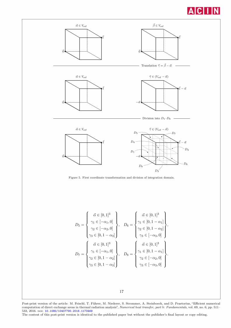
are symmetric in the sense that g(~γ) = g(−~γ) and f(~α, ~β) = f(~β, ~α), respectively. As

outlined in Fig. 5, we first substitute ~β = ~α+ ~γ. Then,

vivi =

∫

Vref

∫

(Vref−~α)k(~α, ~α+ ~γ) d~γ d~α, (24)

where Vref − ~α denotes the set Vref shifted by −~α. Clearly, we have a singular behavior

as ~γ → (0, 0, 0). This is why we split the 6-dimensional integration domain into eight

non-overlapping subdomains around ~γ = (0, 0, 0) (see Fig. 5). These domains are given

by

D1 =

~α ∈ [0, 1]3

γ1 ∈ [−α1, 0]

γ2 ∈ [−α2, 0]

γ3 ∈ [−α3, 0]

, D2 =

~α ∈ [0, 1]3

γ1 ∈ [0, 1 − α1]

γ2 ∈ [0, 1 − α2]

γ3 ∈ [0, 1 − α3]

,

D3 =

~α ∈ [0, 1]3

γ1 ∈ [−α1, 0]

γ2 ∈ [0, 1 − α2]

γ3 ∈ [−α3, 0]

, D4 =

~α ∈ [0, 1]3

γ1 ∈ [0, 1 − α1]

γ2 ∈ [−α2, 0]

γ3 ∈ [0, 1 − α3]

,

16


http://dx.doi.org/10.1080/10407790.2016.1173469

~α ∈ Vref

~α ∈ Vref

~α ∈ Vref

~1

~1

~1~1

~0

~0 ~0

~0

~β ∈ Vref

~γ ∈ (Vref − ~α)

~γ ∈ (Vref − ~α)

−~α

−~α

D1D2

Translation ~γ = ~β − ~α

Division into D1–D8

~1− ~αD4

D5 D7

D8

D3

D6

~1− ~α

Figure 5. First coordinate transformation and division of integration domain.

D5 =

~α ∈ [0, 1]3

γ1 ∈ [−α1, 0]

γ2 ∈ [−α2, 0]

γ3 ∈ [0, 1 − α3]

, D6 =

~α ∈ [0, 1]3

γ1 ∈ [0, 1 − α1]

γ2 ∈ [0, 1 − α2]

γ3 ∈ [−α3, 0]

,

D7 =

~α ∈ [0, 1]3

γ1 ∈ [−α1, 0]

γ2 ∈ [0, 1 − α2]

γ3 ∈ [0, 1 − α3]

, D8 =

~α ∈ [0, 1]3

γ1 ∈ [0, 1 − α1]

γ2 ∈ [−α2, 0]

γ3 ∈ [−α3, 0]

.

17


http://dx.doi.org/10.1080/10407790.2016.1173469

and satisfy⋃8

j=1Dj = Vref × (Vref − ~α). Thus, the integral vivi changes to

vivi =

8∑

j=1

∫

Dj

k(~α, ~α+ ~γ) d~γ d~α. (25)

γ1

α1

−γ1

D2

D1

1

1

0

−1

Figure 6. Parametrization of the integration domain Vref × (Vref − ~α) required for changing the order of integra-tion, where only the first components (γ1, α1) are visualized.

The domains D1 and D2 (cf. Fig. 6) can equivalently be written as

D1 =

~γ ∈ [−1, 0]3

α1 ∈ [−γ1, 1]

α2 ∈ [−γ2, 1]

α3 ∈ [−γ3, 1]

, D2 =

~γ ∈ [0, 1]3

α1 ∈ [0, 1 − γ1]

α2 ∈ [0, 1 − γ2]

α3 ∈ [0, 1 − γ3]

. (26)

18


http://dx.doi.org/10.1080/10407790.2016.1173469

D1

~1

~1 ~1

~1 ~1~1

~1

~1~1~1

~1

~1

~1

~1

~1~1

~α ∈ [0, 1−γ1]×[0, 1− γ2]

−~γ

~0

~0 ~0

~0 ~0~0

~0

~0

~0~0~0

~0

~0

~0

~0

~0~0

~γ ∈ −Vref

Coordinate transformation ~γ → −~γ

D2

~γ ∈ Vref~γ ∈ Vref

~γ ∈ Vref

~γ ∈ Vref

~1− ~γ

Coordinate transformation ~α → ~α− ~γ

~γ

~γ

~γ

~γ

g(~γ), f(~α, ~α+ ~γ)g(~γ), f(~α, ~α+ ~γ)

g(~γ) = g(−~γ), f(~α, ~α− ~γ)

W1 W2 W3

W

−~1

g(~γ), f(~α− ~γ, ~α) = f(~α, ~α− ~γ)

~µ ∈ Vref ~ν ∈ VrefΦ−1

1 (~γ, ~α)

~α ∈ [γ1, 1]×[γ2, 1]× [γ3, 1]

~α ∈ [γ1, 1]×[γ2, 1]× [γ3, 1]

~α ∈ [γ1, 1]×[γ2, 1]× [γ3, 1]

~α ∈ Vref ~γ ∈ D1 ∪D2

D1D2

~α ∈ [−γ1, 1]×[−γ2, 1]

· · · similar for Φ−12 (~γ, ~α) and Φ−1

3 (~γ, ~α)

×[−γ3, 1] ×[0, 1−γ3]

−~α

~1− ~α

~γ ∈ [0, 1]×[0, γ1] ~γ ∈ [0, γ2]×[0, 1] ~γ ∈ [0, γ3]×[0, γ3]×[0, γ1] ×[0, γ2] ×[0, 1]

~α ∈ [γ1, 1]×[γ2, 1]×[γ3, 1]

Figure 7. Coordinate transformations.

With symmetry of g and f , the coordinate transformations ~γ → −~γ and ~α → ~α − ~γ

19


http://dx.doi.org/10.1080/10407790.2016.1173469

are applied to D1 and D2, respectively (cf. Fig. 7). We get

∫

D1∪D2

k(~α, ~α+ ~γ) d~γ d~α = 2

∫

[0,1]3g(~γ)

∫ 1

γ1

∫ 1

γ2

∫ 1

γ3

f(~α, ~α− ~γ) dα1 dα2 dα3 d~γ, (27)

as indicated in Fig. 7. In this way, we have transformed the integration over D1 ∪ D2

into an integration over

W =

~γ ∈ [0, 1]3

α1 ∈ [γ1, 1]

α2 ∈ [γ2, 1]

α3 ∈ [γ3, 1]

. (28)

Still, the integrand exhibits a singular behavior for ~γ = (0, 0, 0). To get rid of this

singularity, we will use a special Duffy transformation. To that end, we split the reference

volume Vref = [0, 1]3 for ~γ into three subdomains (pyramides shown in Fig. 7). This gives

the non-overlapping integration domains

W1 =

γ1 ∈ [0, 1]

γ2 ∈ [0, γ1]

γ3 ∈ [0, γ1]

α1 ∈ [γ1, 1]

α2 ∈ [γ2, 1]

α3 ∈ [γ3, 1]

,W2 =

γ1 ∈ [0, γ2]

γ2 ∈ [0, 1]

γ3 ∈ [0, γ2]

α1 ∈ [γ1, 1]

α2 ∈ [γ2, 1]

α3 ∈ [γ3, 1]

,W3 =

γ1 ∈ [0, γ3]

γ2 ∈ [0, γ3]

γ3 ∈ [0, 1]

α1 ∈ [γ1, 1]

α2 ∈ [γ2, 1]

α3 ∈ [γ3, 1]

, (29)

which satisfy W = W1 ∪W2 ∪W3. Each of these subdomains will then be transformed

back to the reference volume Vref by a special Duffy transformation. Moreover, we will

also transform the volume [γ1, 1]× [γ2, 1]× [γ3, 1] to Vref .

Let Φj with j = 1, 2, 3 denote the functions which transform Vref × Vref = [0, 1]6 into

the domains Wj. The meaning of Φ1 is indicated in Fig. 7. With ~µ = (µ1, µ2, µ3) ∈ Vref

and ~ν = (ν1, ν2, ν3) ∈ Vref , the functions Φj are given by

Φ1(~µ, ~ν) = (µ1, µ1µ2, µ1µ3, µ1 + ν1(1− µ1), µ1µ2 + ν2(1 − µ1µ2), µ1µ3 + ν3(1− µ1µ3)),

Φ2(~µ, ~ν) = (µ1µ2, µ2, µ2µ3, µ1µ2 + ν1(1− µ1µ2), µ2 + ν2(1− µ2), µ2µ3 + ν3(1− µ2µ3)),

Φ3(~µ, ~ν) = (µ1µ3, µ2µ3, µ3, µ1µ3 + ν1(1− µ1µ3), µ2µ3 + ν2(1− µ2µ3), µ3 + ν3(1− µ3)),

20


http://dx.doi.org/10.1080/10407790.2016.1173469

The corresponding Jacobian determinants are

|det(∇Φ1(~µ, ~ν))| = µ21(1− µ1)(1 − µ1µ2)(1 − µ1µ3), (30a)

|det(∇Φ2(~µ, ~ν))| = µ22(1− µ1µ2)(1− µ2)(1 − µ2µ3), (30b)

|det(∇Φ3(~µ, ~ν))| = µ23(1− µ1µ3)(1− µ2µ3)(1 − µ3). (30c)

According to the transformation theorem and the Fubini theorem, Eq. (27) can be rewrit-

ten in the form

∫

D1∪D2

k(~α, ~α+ ~γ) d~γ d~α = 2

3∑

j=1

∫

Wj

k(~α, ~α − ~γ) d~γ d~α (31)

= 2

3∑

j=1

∫

[0,1]6k(Φj(~µ, ~ν)4,5,6,Φj(~µ, ~ν)4,5,6 − Φj(~µ, ~ν)1,2,3)|det(∇Φj(~µ, ~ν))|d~µ d~ν.

Note that the first three components Φi(~µ, ~ν)1,2,3 of Φi(~µ, ~ν) map to the variable ~γ and

the second three components Φi(~µ, ~ν)4,5,6 of Φi(~µ, ~ν) map to the variable ~α. It remains to

analyze the singularity of the integrand in Eq. (31). We consider the singular part g(~γ)

from Eq. (27) and multiply it with the determinant of the transformations. This leads to

g(Φ1(~µ, ~ν)1,2,3)|det(∇Φ1(~µ, ~ν))|

=exp(−K|(di1µ1, d

i2µ1µ2, d

i3µ1µ3)|)

|(di1µ1, di2µ1µ2, di3µ1µ3)|2µ21(1− µ1)(1− µ1µ2)(1− µ1µ3)

=exp(−K|(di1µ1, d

i2µ1µ2, d

i3µ1µ3)|)

|(di1, di2µ2, di3µ3)|2(1− µ1)(1− µ1µ2)(1 − µ1µ3) =: g1(~µ) for µ1 > 0.

For Φ2 and Φ3, we proceed analogously and get

g(Φ2(~µ, ~ν)1,2,3)|det(∇Φ2(~µ, ~ν))|

=exp(−K|(di1µ1µ2, d

i2µ2, d

i3µ2µ3)|)

|(di1µ1, di2, di3µ3)|2

(1− µ1µ2)(1− µ2)(1 − µ2µ3) =: g2(~µ) for µ2 > 0,

g(Φ3(~µ, ~ν)1,2,3)|det(∇Φ3(~µ, ~ν))|

=exp(−K|(di1µ1µ3, d

i2µ2µ3, d

i3µ3)|)

|(di1µ1, di2µ2, di3)|2(1− µ1µ3)(1− µ2µ3)(1− µ3) =: g3(~µ) for µ3 > 0.

Note that the functions g1(~µ), g2(~µ), and g3(~µ) are smooth with respect to ~µ ∈ Vref

because the denominator is strictly positive, i.e., the singularity vanishes by multiplying

g(·) with the Jacobian determinants from Eq. (30).

21


http://dx.doi.org/10.1080/10407790.2016.1173469

Next, we transform the function f(~α, ~α − ~γ) from Eq. (27) by means of the Φk. For a

compact notation, we define the functions fk1 by

fk1 (~µ, ~ν) := f(Φk(~µ, ~ν)4,5,6,Φk(~µ, ~ν)4,5,6 − Φk(~µ, ~ν)1,2,3).

For the remaining domains D3 ∪ D4, D5 ∪ D6, and D7 ∪D8 we proceed similarly. The

functions gk(·) are the same for the other domains but the functions fk1 differ slightly.

We use the notation fk2 for the case D3 ∪D4, f

k3 for D5 ∪D6, and fk

4 for D7 ∪D8.

Finally, the integral from Eq. (25) becomes

vivi =

8∑

j=1

∫

Dj

k(~α, ~α+ ~γ) d~γ d~α = 2

∫

Vref

3∑

k=1

gk(~µ)

∫

Vref

4∑

ℓ=1

fkℓ (~µ, ~ν) d~ν d~µ, (32)

with gk being smooth. However, the functions fkℓ are in general not analytic because

f(~α, ~β) contains the non-analytic factor vis(Λi(~α),Λi(~β)) ∈ {0, 1} (cf. Eq. (22)). For the

special case vis ≡ 1, Eq. (32) simplifies to

vivi =8|Vi|2K2

i

π

∫

Vref

3∑

k=1

gk(~µ) d~µ, (33)

i. e., the 6-fold integral reduces to a 3-fold integral with a smooth integrand.

Generally, the integrals in Eq. (32) are computable with straightforward Gaussian

quadrature from Eq. (19), i.e.,

vivi ≈ 2

3∑

k=1

M∑

k1=0

M∑

k2=0

M∑

k3=0

wk1wk2

wk3gk((sk1

, sk2, sk3

))×

×4∑

ℓ=1

M∑

k4=0

M∑

k5=0

M∑

k6=0

wk4wk5

wk6fkℓ ((sk1

, sk2, sk3

), (sk4, sk5

, sk6)).

3.1.2. Volumes with Positive Distance

Again, we transform the integral (17) to the reference volume Vref using the transforma-

tions Λi and Λj from Section 2.1, i.e.,

vivj =

∫

Vi

∫

Vj

k(~xi, ~xj) d~xi d~xj = |Vi||Vj |∫

Vref

∫

Vref

k(Λi(~α),Λj(~β)) d~β d~α. (34)

The integral kernel k(Λi(~α),Λj(~β)) from Eq. (20) does not have singularities because

|Λi(~α) − Λj(~β)| > 0 for all ~α, ~β ∈ Vref . Therefore, we may straightforwardly apply the

22


http://dx.doi.org/10.1080/10407790.2016.1173469

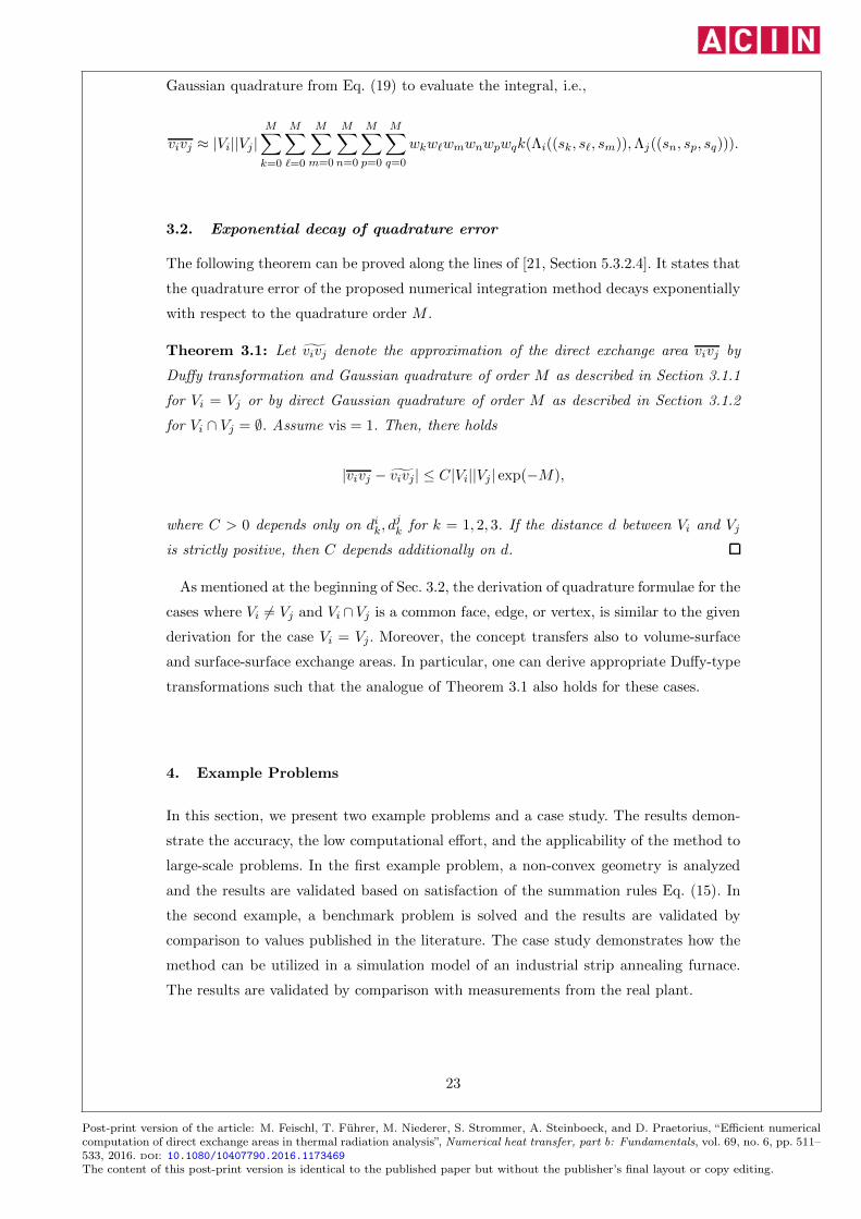
Gaussian quadrature from Eq. (19) to evaluate the integral, i.e.,

vivj ≈ |Vi||Vj |M∑

k=0

M∑

ℓ=0

M∑

m=0

M∑

n=0

M∑

p=0

M∑

q=0

wkwℓwmwnwpwqk(Λi((sk, sℓ, sm)),Λj((sn, sp, sq))).

3.2. Exponential decay of quadrature error

The following theorem can be proved along the lines of [21, Section 5.3.2.4]. It states that

the quadrature error of the proposed numerical integration method decays exponentially

with respect to the quadrature order M .

Theorem 3.1: Let vivj denote the approximation of the direct exchange area vivj by

Duffy transformation and Gaussian quadrature of order M as described in Section 3.1.1

for Vi = Vj or by direct Gaussian quadrature of order M as described in Section 3.1.2

for Vi ∩ Vj = ∅. Assume vis = 1. Then, there holds

|vivj − vivj| ≤ C|Vi||Vj | exp(−M),

where C > 0 depends only on dik, djk for k = 1, 2, 3. If the distance d between Vi and Vj

is strictly positive, then C depends additionally on d.

As mentioned at the beginning of Sec. 3.2, the derivation of quadrature formulae for the

cases where Vi 6= Vj and Vi ∩Vj is a common face, edge, or vertex, is similar to the given

derivation for the case Vi = Vj. Moreover, the concept transfers also to volume-surface

and surface-surface exchange areas. In particular, one can derive appropriate Duffy-type

transformations such that the analogue of Theorem 3.1 also holds for these cases.

4. Example Problems

In this section, we present two example problems and a case study. The results demon-

strate the accuracy, the low computational effort, and the applicability of the method to

large-scale problems. In the first example problem, a non-convex geometry is analyzed

and the results are validated based on satisfaction of the summation rules Eq. (15). In

the second example, a benchmark problem is solved and the results are validated by

comparison to values published in the literature. The case study demonstrates how the

method can be utilized in a simulation model of an industrial strip annealing furnace.

The results are validated by comparison with measurements from the real plant.

23


http://dx.doi.org/10.1080/10407790.2016.1173469

V1

S1

Figure 8. The enclosure of example problem 1 consists of NV = 6 volume zones (left) and the correspondingVS = 22 surface zones, which cover the boundary of the enclosure. For the comparison, we consider the highlightedzones V1 and S1.

4.1. Example Problem 1

We consider the non-convex enclosure outlined in Fig. 8. Direct exchange areas are com-

puted by the proposed method (coordinate transformations and Gaussian quadrature).

For comparison, the problem is also solved by direct application of Gaussian quadrature

(without coordinate transformations).

Because the exchange areas cannot be analytically computed, we check if the summa-

tion rules Eq. (15) are satisfied to validate the obtained results. Therefore, we first select

a volume zone V1 and a surface zone S1 which are highlighted in Fig. 8. We define the

relative error by measuring the relative violation of the summation rules, i.e., for the

volume zone

err(V1) :=

∣∣∣∣∣NV∑

k=1

v1vk +

NS∑

k=1

v1sk − 4K|V1|∣∣∣∣∣/(4K|V1|)

and for the surface zone

err(S1) :=

∣∣∣∣∣NV∑

k=1

vks1 +

NS∑

k=1

s1sk − |S1|∣∣∣∣∣/|S1|,

where v1vk, v1sk, vks1, and s1sk are the approximations of the respective direct exchange

areas. These approximations are obtained by using (first) the quadrature rules from

Section 3 and (second) standard tensor Gaussian quadrature as for the case of non-

touching zones in Section 3.1.2. We will denote the latter approach as the direct approach.

In the case of v1vk and direct tensor Gaussian quadrature, we use M quadrature points

per dimension for the outer three integrals and M + 1 quadrature points per dimension

for the three inner integrals (otherwise the integrand is evaluated at the singularity). The

24


http://dx.doi.org/10.1080/10407790.2016.1173469

2 4 6 8 10

10−10

10−8

10−6

10−4

10−2

100

Order of quadrature M

Relative error err(V1) for volume zone

Duffy + Gauss

Direct Gauss

2 4 6 8 1010−9

10−7

10−5

10−3

10−1

Order of quadrature M

Relative error err(S1) for surface zone

Duffy + Gauss

Direct Gauss

Figure 9. Comparison of example problem 1 in terms of the relative errors err(V1) and err(S1) of the summationproperty Eq. (15) using either the presented quadrature rules (Duffy + Gauss) or standard Gaussian quadrature

rules (direct Gauss).

comparison is shown in Fig. 9.

We observe a significant improvement for the volume zone and for the surface zone. The

direct quadrature does not even seem to converge for the surface zone. This underlines

the necessity of using proper quadrature formulas to evaluate singular integrals.

4.2. Example Problem 2

For simple rectangular geometries consisting of cubes (NV = 2 volume zones) and squares

(NS = 10 surface zones), exchange areas can be found in published tables and charts, see

[1, 10, 12, 25]. In the following, a simple example of an industrial furnace presented in [10]

is used as a benchmark. In this example, the exchange area vsL between a participating

gaseous medium in the rectangular furnace chamber represented by V1 and V2 and the

load represented by the gray surface sections is determined (cf. Fig. 10). The accuracy

of the result is checked based on values published in [10] and based on the summation

rules Eq. (15).

As outlined in Fig. 10, the discretized geometry of the considered furnace chamber

consists of two adjacent cubic gas volumes bounded by square surface zones with a

side length of B = 2m. This discretization is chosen based on the available exchange

areas published in [10]. The gas is assumed to have a constant absorption coefficient

K = 0.16m−1. The load is shown as a gray shaded surface. Selected exchange areas

required for determining the radiative heat transfer inside the enclosure are given in

Tab. 1. The left column contains the exchange areas presented in [10]. The exchange

area v1v1 cannot be directly determined from [10] because of the associated singularities.

25


http://dx.doi.org/10.1080/10407790.2016.1173469

B

B

B

V1 V2

S1

S2

S3

S4

S5

S6

Furnace chamber

Load

Figure 10. Discretized rectangular furnace chamber from example problem 2.

If required, this exchange area may be determined by using the summation rules Eq. (15).

The right column contains the results obtained by using the proposed integration method

with M = 10 quadrature points. The results agree very well with those from [10].

Table 1. Selected direct exchange areasfor the enclosure from example problem 2(cf. Fig. 10).

[10] Duffy + Gauss

s1s2 0.67742 0.67410

s1s3 0.56111 0.56063

s1s4 0.11911 0.11911

s1s5 0.22709 0.22581

s1s6 0.07967 0.07968

s2s6 0.14144 0.14136

v1v2 0.12084 0.12084

v1v1 - 0.66222

v1s1 0.74611 0.74296

v1s6 0.09975 0.10054

v2s1 0.13078 0.13040

Taking into account the symmetry of the considered geometry and using the reciprocity

rules Eq. (14), the desired exchange area vsL can be determined by vsL = 2v1s1+2v2s1.

Thus, we obtain vsL = 1.7538m2 according to [12] and vsL = 1.7467m2 from the

26


http://dx.doi.org/10.1080/10407790.2016.1173469

developed integration method. To verify both results, the summation rule

SL = sLsL + sW sL + vsL (35)

is checked. Here, SL is the surface area of the load, sLsL = 0 is the self-interaction

of the load, and sW sL = 6s1s2 + 2s1s3 + 4s1s4 + 2s1s5 + 2s1s6 is the exchange area

between the remaining surfaces and the load. Using the results from [12], Eq. (35) yields

SL = 8.03m2, which is close to the true value of the surface area 8m2. With the proposed

integration method, the surface area SL = 8m2 according to Eq. (35) matches exactly

the real value, i.e., the summation rule is exactly fulfilled. This result demonstrates the

high accuracy of the developed integration method that systematically takes into account

the singularities.

We stress that the proposed method is not limited to cubes and squares, i.e. the desired

exchange area vsL can also be directly determined by applying the proposed method

to the corresponding 5-fold integral (9). This example was presented for benchmark

purposes. In the next section, a more challenging radiation enclosure with obstacles is

analyzed. For this geometry, we cannot simply use tabulated exchange areas from the

literature.

4.3. Case Study - Industrial Furnace

We consider a direct-fired continuous strip annealing furnace, where steel strips are

heated by means of hot flue gas which stems from the combustion of natural gas

[26, 27, 28]. The flue gas contains molecules like water and carbon dioxide, which have

non-symmetrical oscillation patterns [3]. This is why the flue gas constitutes a partici-

pating medium and has to be considered in an analysis of the radiative heat exchange.

Thermal radiation is the dominant heat transfer mechanism in this furnace due to the

high temperatures [11]. For a simulation model of the considered furnace, the radiative

heat transfer should be accurately captured. To avoid the effort of computing direct ex-

change areas for the zone method, various simplified approaches have been proposed in

the literature on furnace modeling [27, 29, 30]. In [27], for example, furnaces are consid-

ered as tubes and are discretized in the longitudinal direction into finite volume zones.

In each volume zone, the radiative heat transfer is modeled by a local radiation bal-

ance with simplified two-dimensional direct exchange areas [31], i.e., there is no radiative

interaction in the longitudinal direction.

A simulation model of the furnace considered here has been presented in [28]. Based on

this model, the capabilities of the proposed method for calculating direct exchange areas

27


http://dx.doi.org/10.1080/10407790.2016.1173469

are demonstrated. To that end, two versions of the model are considered: In version 1,

the zone method is applied and the integration method proposed in this paper is used to

calculate the direct exchange areas. That is, thermal radiation is considered as a three-

dimensional problem in version 1 of the model. In version 2 of the model, radiative heat

transfer is modeled as a two-dimensional problem as proposed in [27].

Fig. 11 shows the considered furnace of voestalpine Stahl GmbH, Linz, Austria, which

is characterized by the parameters listed in Tab. 2. The counterflow furnace consists of

Table 2. Parameters of the furnace from the casestudy.

Parameter Value

Strip velocity 90− 180m/min

Strip thickness 0.35 − 1.2mm

Strip width 800 − 1700mm

Length of furnace 50m

a preheater, a post combustion chamber, and four heating zones A–D with gas burners.

Due to the combustion of natural gas, energy is released and the strip is heated. The

strip is conveyed through the furnace by three rolls. At the end of the furnace, the strip

temperature is measured by a pyrometer. Additionally, thermocouples are installed in

the heating zones to measure the local wall temperatures.

In Sec. 4.3.1, an overview of the simulation model is given. A simulation study is carried

out based on both versions of the model. In Section 4.3.2, the model is verified by means

of measurements from the real plant.

4.3.1. Overview of the Simulation Model

The proposed furnace model (cf. [28]) consists of submodels for the combustion, the flue

gas, the rolls, the strip, and the walls. These submodels are interconnected by means

of the heat transfer mechanisms conduction, convection, and radiation, see Fig. 12. The

furnace has been discretized into volume zones, which are considered as well-stirred

reactors. In the submodels, the mass, the enthalpy, and the heat balance as well as

chemical reaction equations have been applied to capture the dynamic behavior and

thermal radiation has been modeled by the zone method. The flue gas volume constitutes

the volume zones. The rolls, the strip, and the walls constitute the surface zones. The

submodels are assembled to a dynamical model, which can be written in the state-space

28


http://dx.doi.org/10.1080/10407790.2016.1173469

aaaaaaaaaaaaaa

aaaaaaaaaaaaaa

aaaaaaaaaaaaaaaaaaaaaaaaaaaaaaaaaaaaaaaaaaaa

aa

aaaaaaaaaaaaaaaaaa

aaaaaaaaaaaaaaaaaaaa

aaaaaaaaaaaaaaaaaaaaaaaaaaaaaaaaaaaaaaaa

aaaaaaaaaaaaaaaaaa

aaaaaaaaaaaaaaaaaaaaaaaaaaaaaa

aaaaaaaaaaaaaaaaaaaaaaaaaaaaaaaaaa


aaaaaaaaaaaaaa

aaaaaaaaaaaaaaaaaaaaaa


aaaaaaaaaaaaaaaaaaaaaaaaaaaaaaaaaaaaaaaaaaaaaaaaaaaaaaaaaaaaaaaaaaaaaaaaaaaaaaaaaaaa

aaaaaaaaaaaaaaaaaaaaaaaaaaaaaa

aaaaaaaaaaaaaaaa

aaaaaaaaaaaaaaaaaaaaaaaaaaaaaaaaaaaaaaaaaaaaaaaaaaaaaaaaaaaaaaaaaaaaaaaaaaaaaaaaaaaaaaaaaaaaaaaaaaaaaaaaaaaaaaaaaaaaaaaaaaaaaaaaaaaaaaaaaaaaaaaaaaaaaaaaaaaaaaaaaaaaaaaaaaaaaaaaaaaaaaaaaaaaaaaaaaaaaaaaaaaaaaaaaaaaaaaaaaaaaaaaaaaaaaaaaaaaaaaaaaaaaaaaaaaaaaaaaaaaaaaaaaaaaaaaaaaaaaaaaaaaaa

aaaaaaaaaaaaaaaaaaaaaa

aaaaaaaaaaaaaaaaaaaaaaaaaaaaaaaaaaaaaaaaaaaa

aaa aa

aaaa

aaaaaa

Hot strip

Heating zone A

Heating zone B

Gas flow

Heating zone C

Heating zone D

Preheater

Post combustion

Roll

Funnel

Cold strip

Strip

Wall

Strip motion

BurnerPyrometer

chamber

Figure 11. Schematic of the strip annealing furnace [28] analyzed in the case study.

form

d

dτx = f(τ,x,u) (36)

(cf. [28]) with the time τ and the state vector x. Eq. (36) also captures the heat flows

due to thermal radiation. Moreover, the system input u includes the air and fuel supply

to the burners, the strip velocity, the strip thickness and width, and the steel grade.

4.3.2. Verification of the Simulation Model

The simulation results have been computed by both versions of the considered math-

ematical model and are compared to data recorded at the real plant. Fig. 13 shows a

comparison of the strip temperature at the end of the furnace, where the pyrometer is

29


http://dx.doi.org/10.1080/10407790.2016.1173469

Chemical reactions

Balance equations for

Combustion

Roll

mass and enthalpy Flue gas

Heat balance

Heat balance

Heat balance

Conduction

Radiation

Strip

Convection

Wall

Zone method

Figure 12. Submodels of the furnace considered in the case study.

located. This figure indicates the good accuracy achieved by the furnace model version 1,

0 0.5 1 1.5 2

800

850

900

τ in h

t sin

K

Measurement Model version 1 Model version 2

Figure 13. Strip temperature at the end of the furnace considered in the case study.

where both the steady-state and the transient operation are well captured. Version 2 is

characterized by a similar dynamical behavior, however, an offset occurs. Fig. 14 shows a

comparison of the simulated and the measured wall temperature tw in the heating zone

C. These results demonstrate the good accuracy achieved by both versions of the fur-

nace model. However, version 1 performs better than version 2 due to the more detailed

submodel of the radiative heat transfer. This case study demonstrated the benefit of the

proposed integration method for an industrial scenario.

30


http://dx.doi.org/10.1080/10407790.2016.1173469

0 0.5 1 1.5 21400

1450

1500

1550

τ in h

t win

K

Measurement Model version 1 Model version 2

Figure 14. Wall temperature in the heating zone C of the furnace considered in the case study.

5. CONCLUSIONS

The original results and findings of this work are the following: We derived coordinate

transformations for the calculation of direct exchange areas which distribute points with

singularities to larger domains. This eliminates the singularities, leads to smooth kernels,

and allows for a rigorous mathematical analysis of the quadrature error. The approach is

an effective cure for the significant and so-far unsolved problem of singularities in the cal-

culation of direct exchange areas. The proposed method can treat non-convex geometries

which require the consideration of a visibility function as mentioned in Section 2.2. Here,

the computational load can be reduced if geometry elements are hierarchically clustered.

In case of constant visibility (i.e. vis = 1), the integral reduces to a lower dimensional

integral. The developed method was validated based on numerical results, results pub-

lished in the literature, and measurements from an industrial plant. The method is not

restricted to the computation of direct exchange areas and may be utilized in a similar

way for more general singular integral kernels.

ACKNOWLEDGMENT

This research was financially supported by the Austrian Research Promotion Agency

(FFG), grant no.: 834305. Moreover, the authors are grateful to the industrial re-

search partners voestalpine Stahl GmbH and Andritz AG. The research of the au-

thors MF, TF, and DP is supported through the FWF project Adaptive Boundary El-

ement Method, funded by the Austrian Science fund (FWF) under grant P21732, see

http://www.asc.tuwien.ac.at/abem. The authors MF and DP acknowledge the sup-

port of the FWF doctoral program “Dissipation and Dispersion in Nonlinear PDEs”

under grant W1245, see http://npde.tuwien.ac.at/. The author AS gratefully ac-

31


http://dx.doi.org/10.1080/10407790.2016.1173469

knowledges financial support provided by the Austrian Academy of Sciences in the form

of an APART-fellowship at the Automation and Control Institute of Vienna University

of Technology.

REFERENCES

1. H.C. Hottel and E.S. Cohen. Radiant heat exchange in a gas filled enclosure: Allowance for

non-uniformity of gas temperature. American Institute of Chemical Engineering Journal,

4:3–14, 1958.

2. R. Siegel and J.R. Howell. Thermal Radiation Heat Transfer. Taylor & Francis, New York,

London, 4th edition, 2002.

3. M.F. Modest. Radiative Heat Transfer. Academic Press, New York, 2nd edition, 2003.

4. H.C. Hottel and A.F. Sarofim. Radiative Transfer. McGraw-Hill, New York, 1967.

5. H.D. Baehr and K. Stephan. Heat and Mass Transfer. Springer, Berlin Heidelberg, 2nd

edition, 2006.

6. A. Faghri, Y. Zhang, and J.R. Howell. Advanced Heat and Mass Transfer. Global Digital

Press, Columbia, MO, 2010.

7. J.R. Howell. Thermal radiation in participating media: The past, the present, and some

possible futures. Transactions of the ASME, Journal of Heat Transfer, 110(4b):1220–1229,

1988.

8. Y.S. Kocaefe, A. Charette, and M. Munger. Comparison of the various methods for analysing

the radiative heat transfer in furnaces. Proceedings of the Combustion Institute Canadian

Section Spring Technical Meeting, Vancouver, Canada, pages 15–17, May 1987.

9. S.C. Mishra and M. Prasad. Radiative heat transfer in participating media – A review.

Sadhana - Academy Proceedings in Engineering Sciences, 23(2):213–232, 1998.

10. J.M. Rhine and R.J. Tucker. Modelling of Gas-Fired Furnaces and Boilers and Other Indus-

trial Heating Processes. McGraw-Hill, London, UK, 1991.

11. R. Viskanta and M.P. Menguc. Radiation heat transfer in combustion systems. Progress in

Energy and Combustion Science, 13(2):97–160, 1987.

12. R.J. Tucker. Direct exchange areas for calculating radiation transfer in rectangular furnaces.

Transactions of the ASME, Journal of Heat Transfer, 108(3):707–710, 1986.

13. H. Errku. Radiant heat exchange in gas-filled slabs and cylinders. PhD thesis, Massachusetts

Institute of Technology, Cambridge, MA, 1959.

14. W. Tian and W.K.S. Chiu. Calculation of direct exchange areas for nonuniform zones us-

ing a reduced integration scheme. Transactions of the ASME, Journal of Heat Transfer,

125(5):839–844, 2003.

15. J. Sika. Evaluation of direct-exchange areas for a cylindrical enclosure. Transactions of the

ASME, Journal of Heat Transfer, 113(4):1040–1044, 1991.

16. W. Tian and W.K.S. Chiu. Hybrid method to calculate direct exchange areas using the

32


http://dx.doi.org/10.1080/10407790.2016.1173469

finite volume method and midpoint intergration. Transactions of the ASME, Journal of

Heat Transfer, 127(8):911–917, 2005.

17. J.C. Chai, J.P. Moder, and K.C. Karki. A procedure for view factor calculation using the

finite-volume method. Numerical Heat Transfer, Part B: Fundamentals, 40(1):23–35, 2001.

18. H. Ebrahimi, A. Zamaniyan, J.S.S. Mohammadzadeh, and A.A. Khalili. Zonal modeling

of radiative heat transfer in industrial furnaces using simplified model for exchange area

calculation. Applied Mathematical Modelling, 37(16-17):8004–8015, 2013.

19. A. Kheiri, J.L. Tanguier, D. Bour, R. Mainard, and J. Kleinclauss. Transfert de chaleur dans

les milieux semi-transparents: adaptation de la methode des zones de Hottel aux milieux

optiquement epais. Proceeding of the SFT-90 Colloque de Thermique, Nantes, France, 2:37–

40, May 1990.

20. J.M. Goyheneche and J.F. Sacadura. The zone method: A new explicit matrix relation to

calculate the total exchange areas in anisotropically scattering medium bounded by anisotrop-

ically reflecting walls. Transactions of the ASME, Journal of Heat Transfer, 124(4):696–703,

2002.

21. S.A. Sauter and C. Schwab. Boundary Element Methods, volume 39 of Springer Series in

Computational Mathematics. Springer-Verlag, Berlin, 2011.

22. L. Greengard and V. Rokhlin. A fast algorithm for particle simulations. Journal of Compu-

tational Physics, 73(2):325–348, 1987.

23. H. Cheng, L. Greengard, and V. Rokhlin. A fast adaptive multipole algorithm in three

dimensions. Journal of Computational Physics, 155(2):468–498, 1999.

24. S. Borm, L. Grasedyck, and W. Hackbusch. Introduction to hierarchical matrices with ap-

plications. Engineering Analysis with Boundary Elements, 27(5):405 – 422, 2003.

25. H.B. Becker. A mathematical solution for gas-to-surface radiative exchange area for a rectan-

gular parallelepiped enclosure containing a gray medium. Journal of Heat Transfer, 99:203–

207, May 1977.

26. K.S. Chapman, S. Ramadhyani, and R. Viskanta. Modeling and analysis of heat transfer in a

direct-fired continuous reheating furnace. Heat Transfer In Combustion Systems, 122:35–44,

1989.

27. D. Marlow. Modelling direct-fired annealing furnaces for transient operations. Applied Math-

ematical Modelling, 20(1):34–40, 1996.

28. S. Strommer, M. Niederer, S. Steinboeck, and A. Kugi. A mathematical model of a direct-

fired continuous strip annealing furnace. International Journal for Heat and Mass Transfer,

69:375–389, 2014.

29. A. Jaklic, F. Vode, and T. Kolenko. Online simulation model of the slab-reheating process

in a pusher-type furnace. Applied Thermal Engineering, 27:1105–1114, 2007.

30. C.-K. Tan, J. Jenkins, J. Ward, J. Broughton, and A. Heeley. Zone modelling of the ther-

mal performances of a large-scale bloom reheating furnace. Applied Thermal Engineering,

50:1111–1118, 2013.

31. J.P. Holman. Heat Transfer, volume 10. McGraw Hill, 2010.

33


http://dx.doi.org/10.1080/10407790.2016.1173469

Date post:	02-May-2018
Category:	Documents
Upload:	trankhue
View:	215 times
Download:	0 times

Eﬃcientnumericalcomputationofdirectexchangeareasinthermal … · ·...

Documents