Eco 300 Intermediate Micro - State University of New …aj4575/eco300_2010/Lecture... · Eco 300...

Eco 300 Intermediate Micro

Instructor: Amalia Jerison

Office Hours: T 12:00-1:00, Th 12:00-1:00,and by appointment

BA 127A, [email protected]

A. Jerison (BA 127A) Eco 300 Spring 2010 1 / 37

Illustration of the Substitution Effect: A Gasoline Tax with aRebate

Suppose the US government considers taxing gasoline to reducegasoline consumption.

The government wants to give the tax revenue back to consumersas a rebate.

What are the effects on a consumer?


Focus on a period of 5 years

Over this period, the price elasticity of demand is approximately−0.5

Because the elasticity of demand is low, and the elasticity ofsupply is relatively high, most of tax passed on to buyers.

Thus, to simplify, assume that the entire tax is passed on tobuyers.


Consider a 50 cent per gallon tax.

A certain average consumer initially buys 1200 gallons gas peryear.

Gasoline initially costs $1.00 per gallon.

The consumer’s annual income is $9000.


Budget line is AB

Initially the consumer chooses point C.

She buys 1200 gallons gas, spends $7800 on other goods.


Gasoline(gallons perYear)

ExpendituresOn otherGoods ($)

1200

7800C

A

B


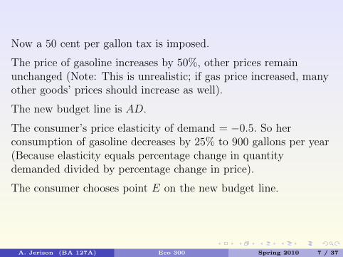
Now a 50 cent per gallon tax is imposed.

The price of gasoline increases by 50%, other prices remainunchanged (Note: This is unrealistic; if gas price increased, manyother goods’ prices should increase as well).

The new budget line is AD.

The consumer’s price elasticity of demand = −0.5. So herconsumption of gasoline decreases by 25% to 900 gallons per year(Because elasticity equals percentage change in quantitydemanded divided by percentage change in price).

The consumer chooses point E on the new budget line.




C

A

BD

E

900


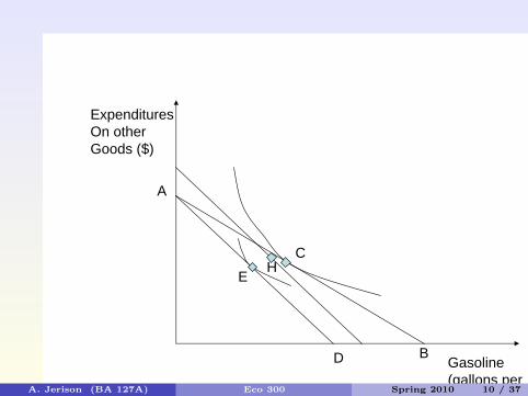
The rebate program comes into effect.

Tax revenue is about 900 × $0.50 = $450 per person (because theconsumer considered was an average consumer of gasoline).

This will be given back as a lump sum to each consumer.

So our consumer’s income increases by $450 per year.

The new budget line, FJ , is AD shifted parallel to the right




C

A

BD

EH


Suppose the income elasticity of demand for gasoline isapproximately 0.3.

Gasoline consumed increases by (450/9000) × 0.3 × 900 = 13.5gallons (because income elasticity equals percentage change inquantity demanded divided by percentage change in income),

to 913.5 gallons per year.

Now the consumer is at point H on budget line FJ .

This is less than the original amount of gasoline consumed.

The consumer in on a lower indifference curve than she wasoriginally.


Her consumption of gasoline has been reduced due to thetax-rebate.

This consumer was made worse off by the tax-rebate.

Other consumers may be made better off if they originallyconsume less gasoline than the average.

But on average consumers are made worse off due to thedistorting effect of the tax.

Whenever there is a tax with a lump-sum compensation, theaverage consumer will be made worse off if there are nopreexisting distortions (such as externalities).


However, this may not be true with an externality.

Gasoline generates a negative externality.

When you take into effect the benefits of less pollution due to lessgas consumption, the average consumer may be better off.


From individual to market demand

Market demand is determined as the sum of individuals’ demandsat each price.

On graph, sum horizontally all individuals’ demand curves.

Even if all individual demands are linear, the market demand maybe non-linear (it may be kinked).


D1 D2 D3

Q

P


Market demand curves can be built up by adding the demandcurves of different demographic groups.

For instance, there may be information about domestic demandfor wheat and foreign demand for wheat. Add these demandcurves to get the total demand for wheat.


The aggregate demand for US wheat

The domestic demand for wheat is given by the equation

QDD = 1430 − 55P ,

where QDD is the number of millions of bushels demandeddomestically, and P is the price in dollars per bushel.

The foreign demand for wheat is given by the equation

QDE = 1470 − 70P


Domestic demand is relatively price inelastic (dQ/dP = −55, so(dQ/dP )(P/Q) = −55(P/Q).

Statistical studies have shown that price elasticity of domesticdemand is about −0.2 to −0.3.

Export demand is more price elastic; elasticity is about −0.4.

This could be because poorer countries that import US wheatswitch to other grains when wheat becomes more expensive.


Add the two quantities for any given price.

QDD + QDE = (1430 − 55P ) + (1470 − 70P ) = 2900 − 125P .

This is the equation of the total demand curve for prices below 21per bushel.

For prices above 21, the export demand is zero. So the sum of thetwo demand curves equals the domestic demand curve.

So the equation for total demand is

QD = 2900 − 125P , P < 21

QD = 1430 − 55P , P ≥ 21


The demand for housing

On average, households spend 25 percent of income on housing.

Demand for housing depends on age and status of household.

Government wants to estimate elasticity of housing demand topredict effectiveness of subsidies for low-income families, rentcontrols and land-use regulation.

There are differences in elasticities among different groups.


Families with young household heads have a price elasticity of−0.25.

Families with older household heads have lower price elasticity of−0.15 for household heads aged 30 to 39 and 2 or more children.

Families with household heads age 50 or older with 1 child haveprice elasticity of −0.08.


For poor households (incomes in bottom tenth percentile), incomeelasticity of housing is only 0.09. This implies that incomesubsidies would be spend primarily on goods other than housing.

Income elasticity for housing among top 10 percent wealthiesthouseholds is around 0.54.


Consumer surplus

Consumer surplus measures how much better off consumers aredue to a purchase, compared to not purchasing the item.

An individual’s consumer surplus can be measured in this way:

Suppose the individual values a good at $15 i.e. would be willingto pay up to $15 for it.

However the price of the good is $12.

Then the individual’s consumer surplus is $3.

Total consumer surplus is sum of individuals’ consumer surpluses.


An example: Draw one person’s demand curve for tickets as astaircase because tickets are indivisible - one can only buy themin integer amounts.

Suppose tickets to a concert cost $14.

Suppose to the person, the first ticket bought is worth $20, thesecond worth $19, the third worth $18, the fourth worth $17, thesixth worth $16 and the seventh worth $15 and so on.

then buying the first ticket generates a consumer surplus of $6,buying the second ticket generates a consumer surplus of $5 andso on.


Thus consumer will buy 7 tickets. For the seventh, they areindifferent about buying it or not. We just assume they buy whenindifferent.

Will not buy any more than 7 because the price will be greaterthan the value.

The total consumer surplus is 6 + 5 + 4 + 3 + 2 + 1 = $21.

To calculate market consumer surplus, calculate area above priceline below market demand curve


Market Price

Consumersurplus

Expenditure

Q

P


Network Externalities

Exist when people’s demand for a good depends on how manyother people are consuming that good.

Bandwagon effect - people demand more of a good when a lot ofpeople are consuming it.

It is a positive network externality, associated with fads and beingin style.


Other positive network externalities exist:

e.g. the value of a CD player is higher the more people own CDplayers because more CD’s made when more people own CDplayers.

The value of a computer is higher the more people own computersbecause more software gets written.


Snob effect- people demand more of a good when few people areconsuming it.

This is a negative network externality.


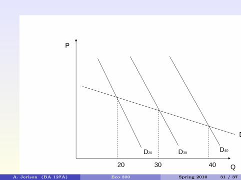
Bandwagon effect- an example of positive network externality

Shown in graph - horizontal axis shows sales of good in thousandsper month.

D20 shows the demand curve when consumers think only 20000people have bought the good.

D30 shows the demand curve when consumers think 30000 peoplehave bought the good.

D40 shows the demand curve when consumers think 40000 peoplehave bought the good.etc.


D20 D30 D40

D

20 30 40 Q

P


The demand curve shifts right the more people consumers thinkhave bought the good.

The true demand curve then must be such that 20000 peopleactually buy the good when they think 20000 people have boughtthe good.

To get the true demand curve, start with a quantity Q.

This gives a demand curve when consumers think that Q peopleare buying the good.

Find the price corresponding to that quantity on that demandcurve.

This is the price corresponding to quantity Q


Snob effect - an example of a negative externality

Goods become more valuable because they are rare.

e.g. paintings, etchings, rare editions of books - artists destroyplates after certain number of prints have been made to makeprints more valuable

Any unique producer of a good with no close substitute hasincentive to reduce production when demand inelastic to raiseprice and thus revenue.

With the snob effect, this effect is strengthened because even athigh prices there is an inelastic demand (eventually the demandwill become elastic but at higher prices)


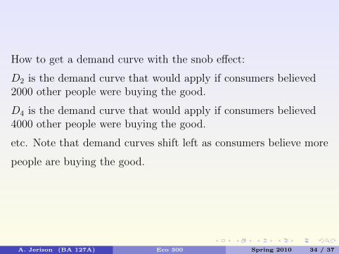
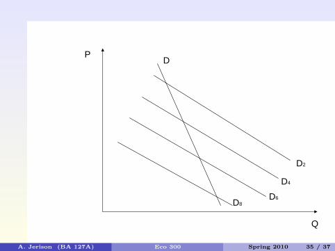
How to get a demand curve with the snob effect:

D2 is the demand curve that would apply if consumers believed2000 other people were buying the good.

D4 is the demand curve that would apply if consumers believed4000 other people were buying the good.

etc. Note that demand curves shift left as consumers believe more

people are buying the good.


D2

D4

D6D8

DP

Q


The true demand curve must be such that people believe Q peopleare buying the good when Q people are actually buying the good.

To get the true demand curve, again start with a quantity Q ofpeople buying the good.

We know the demand curve when people believe that Q peopleare buying the good. Find the price corresponding to thatquantity on the demand curve. That price is the price at which Qpeople will buy the good.


Note that the true demand curve is steeper than any of theconditional demand curves.

Thus it is more likely that the true demand curve is inelastic athigh prices.


Date post:	24-Aug-2018
Category:	Documents
Upload:	lamhanh
View:	217 times
Download:	0 times

Eco 300 Intermediate Micro - State University of New …aj4575/eco300_2010/Lecture... · Eco 300...

Documents