170
ECOLOGY Communities and Ecosystems H.J.B. Birks BIO-201
| Date post: | 01-Jan-2016 |
| Category: |
Documents |
| Upload: | samson-meyers |
| View: | 72 times |
| Download: | 5 times |

ECOLOGY
Communities and Ecosystems
H.J.B. Birks
BIO-201

Communities and Ecosystems
1. Species Abundance, Diversity, & Community Ecology
2. Community Ecology and Dynamics
3. Ecosystem Ecology – Energy Flux
4. Ecosystem Ecology – Matter Flux
5. Long-term Ecology (=Ecological Palaeoecology)
6. Broad-scale Ecology – World Vegetation Biomes
7. Broad-scale Ecology – Landscape & Geographical Ecology
8. Broad-scale Ecology – Species Richness Patterns in Time
9. Broad-scale Ecology – Species Richness Patterns in Space
10.Broad-scale Ecology – Global Earth-System Ecology

1. Species Abundance, Diversity, and Community
Ecology
H.J.B. Birks
BIO-201 ECOLOGY

Species Abundance, Diversity, and Community Ecology
Sub-divisions of ecologyScales in ecologyCommunity level of ecological organisationImportant concepts about community level of organisationThe study of communitiesHow do we quantify the number & relative abundance of species in communities? - Species abundances
- Rank-abundance curves- Species numbers (= richness) and species diversity- Not all species are equal!
What determines diversity? - Environmental complexity- Disturbance and diversity
What determines community structure?Different concepts of the community How to analyse community-scale data?Conclusions and summary

Pensum
The lecture, of course,
and
the PowerPoint handouts of this lecture on the BIO-201 Student Portal
Also ‘Topics to Think About’ on the Student Portal filed under projects

Topics to Think About
On the Bio-201 Student Portal filed under Projects, there are several topics to think about for each lecture. These topics are designed to help you check that you have understood the lecture and to identify important topics for discussion in the Bio-201 colloquia.
In addition, there are two or three more demanding questions at the sort of level you can expect in the examination question based on my 10 lectures. These can also be discussed in the colloquia.

Background Information
There is now a wealth of good or very good ecology textbooks but perhaps no excellent, complete, or perfect textbook of ecology.
Not surprising, given just how diverse a subject ecology is in space and time and all their scales.
This lecture draws on primary research sources, my own knowledge, experience, observations, and studies, and several textbooks.
Textbooks that provide useful background material for this lecture
Begon, M. et al. (2006) Ecology. Blackwell (Chapter 16, parts of Chapters 19 & 20)
Bush, M. (2003) Ecology of a Changing Planet. Prentice Hall (Chapter 15)
Krebs, C.J. (2001) Ecology. Benjamin Cummings (Chapters 20, 22, 23)
Miller, G.T. (2004) Living in the Environment. Thomson (Chapter 8)
Molles, M.C. (2007) Ecology Concepts and Applications. McGraw-Hill (Chapter 16)
Ricklefs, R.E. & Miller, G.L. (2000) Ecology. W.H. Freeman (Chapters 26, 27, 29)
Smith, R.L. & Smith, T.M. (2007) Ecology and Field Biology. Benjamin Cummings (Chapter 20)
Townsend, C.R. et al. (2008) Essentials of Ecology. Blackwell (Chapters 9, 10)

A Reminder
If you try to read Begon, Townsend, and Harper (2006) Ecology – From Individuals to Ecosystems, there is a 17-page glossary of the very large (too large!) number of technical words used in the book on the Bio-201 Student Portal. It can be downloaded from the File Storage folder.
Good luck!

Sub-Divisions of Ecology1. Functional ecology and evolutionary ecology
2. Modern ecology and long-term ecology (=palaeoecology) (the Fourth dimension of ecology)
3. Autecology – study of ecological relationships of a single species
4. Synecology – study of all the species living together as a community (group of plants and animals in a given place forming ecological units of various sizes and degrees of interrelation and integration)
5. Pure and applied ecology
"Pure"– understand, for understanding's sake, the processes responsible for determining the structure and composition of particular assemblages or communities
"Applied"– ecology relevant to food gathering and production, conservation, control of pests and pathogens, pollution, preservation of biodiversity, etc. Includes conservation ecology and restoration ecology.

6. Descriptive ecology – basic patterns of what grows where, what are the environmental variables, and what is the inherent variation in space and time
Explanatory ecology - underlying processes behind observed patterns. Processes may be proximal (near) or ultimate (final)
Predictive ecology – use ecological knowledge and understanding to predict how organisms will respond to environmental changes
7. Observational or field ecology – 'scientific natural history'
Laboratory experimental ecology – 'simplified ecology'
Field experimental ecology – most difficult to do
8. Behavioural ecology – individuals
Population ecology – populations
Community ecology – communities
Landscape ecology – landscapes
Geographical ecology – mappable features
Global ecology – biomes and Earth's systems

Ecology is like a giant and complex jigsaw puzzle
If the organism is not a predator, 'prey' is replaced by 'food' or if the organism is a plant, 'prey' is replaced by 'light and nutrients'.
In addition, an organism competes with other organisms (competitors) for food.
In reality a multi-dimensional (and unsolvable!) jigsaw-puzzle and we do not have all the pieces!

Scales in Ecology
BiosphereBiosphere
landscapes
Communities
Populations
Individual
Biosphere
Biomes e.g. rainforest
Ecosystems & Landscapes
Communities
Species
Populations; breeding individuals
Individual organisms
Biological or hierarchical scales

Atmosphere
Vegetation and animals
Soil
Rock
Biosphere
Crust
core
MantleLithosphere
Crust
Lithosphere(crust, top of upper mantle)
Hydrosphere(water)
Atmosphere(air)
Biosphere(Living and dead
organisms)
Crust(soil and rock)
Global Scale (Lectures 6, 10)
Biosphere
Hydrosphere
(Lithosphere)

15,000 ft10,000 ft5,000 ft
Coastalmountainranges
SierraNevadaMountain
GreatAmericanDesert
RockyMountains
GreatPlains
MississippiRiver Valley
AppalachianMountains
Coastal chaparraland scrub
DesertConiferousforest
Coniferousforest
Prairiegrassland
Deciduousforest
Average annual precipitation
100-125 cm (40-50 in.)
75-100 cm (30-40 in.)
50-75 cm (20-30 in.)
25-50 cm (10-20 in.)
below 25 cm (0-10 in.)
Broad Spatial or Biome Scale (Lecture 6)
World Vegetation Types or Biomes
Role of climate

Landscape Scale
(Lecture 7)
Coast-mountain transition in western Norway

Geographical Scale (Lecture 7)
Alpinetundra
Temperate forest
SEA
Deciduous forest
Montane coniferous forest
Elevation gradient = gradual change

Often no real boundaries between
communities
Populations of different species living and interacting within an ecosystem are referred to collectively as a community
Community Scale (Lectures 1, 2)

Community Boundaries: Often Gradual
Land zone Transition zone Aquatic zone
Numberof species
Species in land zoneSpecies in aquatic zoneSpecies in transition zone only

Deciduous forest and rocky shore = sharp change between communities

Scales of relevance in these ten lectures on Communities and Ecosystems
Community scale (Lectures 1, 2)
Ecosystem (Lectures 3, 4), Landscape (Lecture 7), and Geographical (Lectures 7, 8, 9) scales
Biome scale (Lecture 6)
Biosphere or Global scale (Lecture 10)
plus Time dimension (long-term ecology or palaeoecology) (Lectures 5, 8)

Spatial and Temporal Scales of Biodiversity – closely related
Spatial scale Biological scaleTemporal scale
(years)
LocalPopulations,
communities & habitat patches
1 – 100
Landscape Between communities 100 – 1000
Regional Regions, countries 10,000
Continental Continents 1 – 10 million
GlobalGlobal biodiversity &
biosphere10 – 100 million
BiosphereBiosphere
Ecosystems
Communities
Populations
Organisms
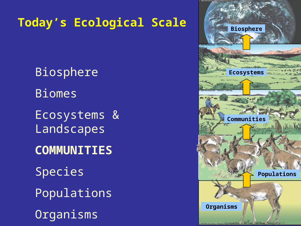
Biosphere
Biomes
Ecosystems & Landscapes
COMMUNITIES
Species
Populations
Organisms
Today’s Ecological Scale

Community Level of Ecological Organisation
'Group of plants and animals in a given place and time forming ecological units of various sizes and degrees of inter-relation and integration.'
Community concept first applied to plants, more recently applied to animals. Most definitions only refer to plants.
'an aggregate of living plants having mutual relations among themselves and to the environment' (Oosting, 1956)
'a collection of plant populations found in one habitat type in one area, and integrated to a degree by competition, complementarity, and dependence' (Grubb, 1987)

Important Concepts about Community Level of Organisation
1. Collections of species which occur together in some common environment or habitat type.
2. Organisms making up the community are somehow integrated and may interact as a unit.
3. Communities are not constructed only of plants.
4. Some communities are mostly animals (e.g. fish and invertebrates that comprise coral-reef communities).
5. Most communities consist of a mixture of plants, animals, fungi, prokaryotes, and protoctists.
6. Population dynamics, distribution and abundance, growth and life histories, competition, predation, herbivory, parasitism, disease, and mutualism provide basic processes within assemblages of living organisms that generate the observed patterns of species diversity, abundance, and composition at the community level.

7. Recognition of communities – two main ways
(a) environment or habitat where community occurs (e.g. lakes, sand-dunes, coastal rock pools)
(b) largest or most abundant or prominent species (e.g. pine forest, oak woodland, grassland, Sphagnum bog)
8. Size of community – no fixed size, can range from very small and constrained (e.g. association of micro-organisms in mammalian gut) to huge expanses of grassland and forest.
9. Why are similar groups of species found again and again in similar habitats?
If the habitat provides a collection of environmental niches and if the same niches occur in similar habitats, then they will be filled by the same species.
Niches for particular plants, grazing animals, decomposers, parasites, etc.

10. Community is built up of species with other dependent species in recognisable combinations.
11. But communities found in a particular habitat type will not be identical. Minor differences in the environment that vary continuously in space and time may occur. Effects of chance or history of the site may mean that some species usually found together are missing and other more unusual species may be present.
12. Species present in a community will vary depending on where in the world the particular community is found. Species growing in coastal pools on rocky shores in Australia will be different from species growing in similar pools in Norway. Hence the importance of biogeography and geographical ecology in determining the available species pool.
13. However, wherever rock pools occur, expect them to have similar relationships between species occupying the same collection of niches.

14. Species that assemble to form a community are determined by (i) dispersal constraints, (ii) environmental constraints, and (iii) internal dynamics.
Species pools:
Total Pool – function of evolution and history
Habitat Pool – function of environmental constraints
Geographic Pool – function of dispersal constraints
Ecological Pool – function of internal dynamics
Community – what remains in face of biotic interactions
The Study of Communities
Within any community there is a complex series of interactions between individuals of different species.
The whole collection of populations may fit together into a functional unit; the community.
Community ecology seeks to understand the way species groupings are distributed in nature and the ways that these groupings are influenced by their abiotic environment (Part I of this course) and by interactions between species populations (Part II)
How do we study communities and understand the complexity of such systems?

1. What is the community structure?
- abiotic features noted (e.g. marine, freshwater, marsh, desert; geology; topography; climate, etc.)
- overall form described (e.g. terrestrial life forms such as trees, shrubs, herbs and grasses, mosses; aquatic mode of locomotion such as free swimmers, planktonic drifters, bottom dwellers, sessile adults)
2. What species are present?
3. How many species live in the community? (Diversity) Is it species-poor or species-rich?
4. What are the abundance patterns of the species?
5. How does the community function? Trophic food webs within the community can be investigated to assess the importance of primary producers, herbivores, predators, and decomposers. This provides data on energy and nutrient cycles. See lectures on Ecosystem Ecology (Lectures 3, 4).
6. What is the influence of the abiotic environment on the composition and structure?
7. How does the community regenerate and sustain itself? Population dynamics and stability (Lecture 2).
8. What is the history of the community? Long-term ecology or palaeoecology (Lecture 5).

No community is well enough studied that we can answer these eight questions!
Overall community structure will be determined by features of the physical environment, community size, longevity of the species present, and history.
Community may be stable or unstable, have low or high primary productivity, and may change seasonally or even daily.
Community, ecosystem, and broad-scale ecology are very difficult to study.
How do we study community ecology?
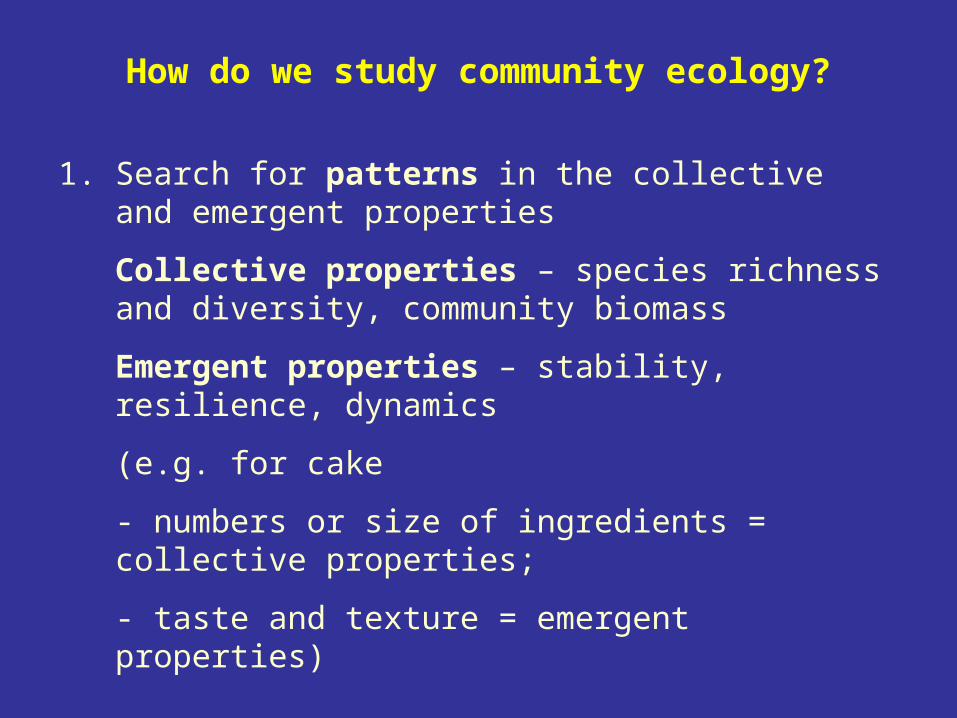
1. Search for patterns in the collective and emergent properties
Collective properties – species richness and diversity, community biomass
Emergent properties – stability, resilience, dynamics
(e.g. for cake
- numbers or size of ingredients = collective properties;
- taste and texture = emergent properties)

2. Patterns are repeated consistencies, such as repeated groupings of similar growth-forms or species in different places, or repeated trends in richness along different environmental gradients.
3. Recognition of patterns leads to formulation of hypotheses about the causes of the patterns, so-called processes.
4. Test hypotheses by making further independent observations or by doing experiments.
5. Much of community ecology is, by necessity, descriptive or narrative, rather than analytical with strict hypothesis testing or statistical modelling.
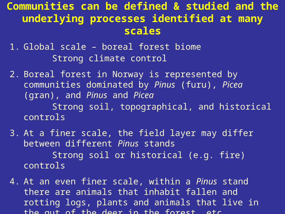
Communities can be defined & studied and the underlying processes identified at many scales
1. Global scale – boreal forest biomeStrong climate control
2. Boreal forest in Norway is represented by communities dominated by Pinus (furu), Picea (gran), and Pinus and Picea
Strong soil, topographical, and historical controls
3. At a finer scale, the field layer may differ between different Pinus stands
Strong soil or historical (e.g. fire) controls
4. At an even finer scale, within a Pinus stand there are animals that inhabit fallen and rotting logs, plants and animals that live in the gut of the deer in the forest, etc.
The scale of investigation depends on the ecological questions being asked.

The structure of oak (Quercus) woodland in spring and summer
Chapman & Reiss

A cross-section of a typical rock pool showing the mixed nature of the community and some of the other organisms which inhabit the more open rocky shore.
Chapman & Reiss

The general structure of the mammalian gut and common members of gut communities (not to scale).
Chapman & Reiss

Often difficult to study large numbers of species, so community ecologists may work with restricted groups, e.g. plants, insects.
Some focus on guilds – group of organisms that all make their living in a similar way (e.g. seed-eating animals in a desert, fruit-eating birds in a forest, filter-feeding invertebrates in a stream). Some guilds consist of closely related species; others may be taxonomically unrelated.
For example, fruit-eating birds on South Pacific Islands are mainly pigeons, whilst the same guild in USA deserts consists of mammals, birds, and ants.
Guild concept mainly used by animal ecologists.
Life-form or growth-form or functional type used by plant ecologists. Combination of structure and growth-dynamics (e.g. trees, vines, annual plants, grasses, herbs (= forbs)). Like an animal guild, plants of similar life-form exploit the environment in similar ways.
By studying animal guilds or plant life-forms, communities can be studied in a more manageable and coherent way than trying to consider all species simultaneously.

All communities have attributes or features that differ from those of the components that make up the community and that only have meaning with reference to the collective assemblage or community.
These attributes are
1. Number of species
2. Relative abundance of species
3. Nature of their interactions
4. Physical structure, defined primarily by the growth-forms of the plant components of the community

How do we Quantify the Number & Relative Abundance of Species in
Communities?
Species Abundances
One of the most striking features of communities is the variation in the relative abundance of species.
Basic questions often asked:
1. For a given community, how many species are there and what are their relative abundances?
2. How many species are rare?
3. How many species are common?

Species abundances are usually based on individuals per species, or variables such as percentage cover or biomass.
Fundamental aspect of community structure – "minimal community structure" (Sugihara, 1980)
What will be found if we go to a community and quantify the abundance of species within a group of taxonomically or ecologically related organisms such as birds, shrubs, herbs, or diatoms?

Species abundance data are arranged in the form of a species abundance distribution, that is a frequency distribution of the number of species with X = 1, 2, 3, … r individuals.
Insect count data from grassland based on 14 sweep nets
X 1 2 3 4 5 6 7 9 10 11 21 28 33 120
f 32 8 9 2 3 3 3 2 1 2 1 1 1 1
X = number of individuals per species
f = frequency of species in each of the X classes
There are 389 individuals and 69 species.

Can we fit a statistical distribution model to such species abundance data?
Hope to find a 'general' model requiring a few, easily estimated and ecologically meaningful parameters.
Turns out that there are regularities in the relative abundance of species in many different communities. If you can thoroughly sample the community, there are usually:
(1) a few very abundant species
(2) a few very rare species
(3) most species have a moderate abundance

Preston "distribution of commonness and rarity" and the log-normal distribution (1948, 1962)
Consider abundance in relative terms and say that one species is twice as abundant as another.
Graph the abundance of species in samples as frequency distribution where the species abundance intervals are 0-1, 1-2, 2-4, 4-8, 8-16, 16-32, etc. individuals, so-called octaves.
Frank Preston
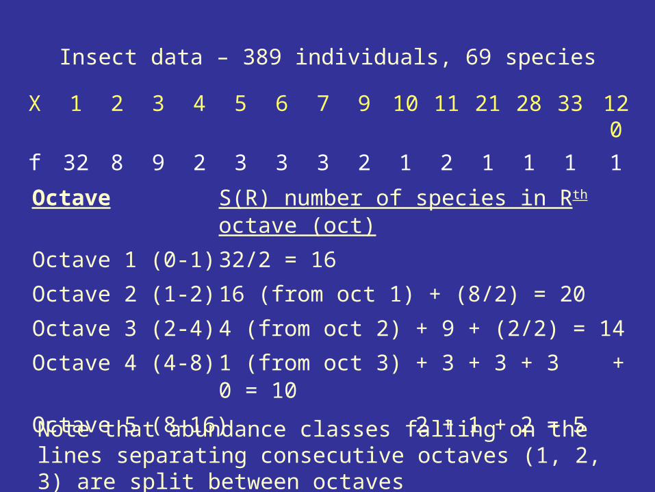
Insect data – 389 individuals, 69 species
X 1 2 3 4 5 6 7 9 10 11 21 28 33 120
f 32 8 9 2 3 3 3 2 1 2 1 1 1 1
Octave S(R) number of species in Rth octave (oct)
Octave 1 (0-1) 32/2 = 16
Octave 2 (1-2) 16 (from oct 1) + (8/2) = 20
Octave 3 (2-4) 4 (from oct 2) + 9 + (2/2) = 14
Octave 4 (4-8) 1 (from oct 3) + 3 + 3 + 3 + 0 = 10
Octave 5 (8-16) 2 + 1 + 2 = 5Note that abundance classes falling on the lines separating consecutive octaves (1, 2, 3) are split between octaves

In Preston log-normal distribution, plot the abundance classes on log2 scale (log2 of 1 = 0, log2 of 2 = 1, log2 of 4 = 2, log2 of 8 = 3, etc.). Each class represents a doubling of the previous abundance class.
Plot log2 of species abundance against the number of species in each abundance interval. Each abundance interval is twice the preceding one.
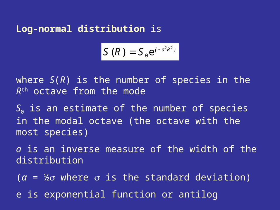
Log-normal distribution is
where S(R) is the number of species in the Rth octave from the mode
S0 is an estimate of the number of species in the modal octave (the octave with the most species)
a is an inverse measure of the width of the distribution
(a = ½ where is the standard deviation)
e is exponential function or antilog
)Ra(SRS22
e)( 0

Estimation of parameters S0 and a
2max
max)()(log
RRSoS
na
where S(o) is the observed number of species in the modal octave and S(Rmax) is the observed number of species in the octave most distant from the modal (indicated by Rmax)
Parameter a has been found to be about 0.2 for a large number of samples in ecology. It has been shown that this ‘rule’ may be a product of the mathematical properties of the log-normal distribution. As the total number of species in the community varies from 20 to 10000, a will vary from 0.3 to 0.13 (assuming that the underlying distribution follows the so-called ‘canonical log-normal’ distribution).

An estimate of S0 is obtained either by fixing it at the observed value for the number of species in the modal octave, S(o), or by estimating it
220 )( loge RaRSS n
where logn S (R) is the mean of the logarithm of the observed number of species per octave, a is estimated as above, and R2 is the mean of all the R2s.

Insect data
Octave No of individuals per
species
Observed S(R)
Expected S(R)
1 0-1 16 14.5
2 1-2 20 15.9
3 2-4 14 15.5
4 4-8 10 11.0
5 8-16 5 6.9
6 16-32 2 3.6
7 32-64 1 1.6
8 64-128 1 1.12 = 2.76; degrees of freedom = octave classes – 2 = 6 Suggests good fit to theoretical log-normal model by observed data.

If communities really follow log-normal distribution, can predict how many species might have been unobserved in the community (S*)
S* = 1.77(S0/a)
where S0 = number of species in modal octave and a is a measure of the curve's width.
In this case S* = 23
In a sample of 389 individuals and 69 species, likely that there are 23 species missed.
Problems of sampling natural assemblages.

Distributions of desert plants and forest birds

Desert plants - few species have cover > 8% or < 0.15%. Most are intermediate
- "bell-shaped" or "normal"
- log scale of cover, so "log-normal"
Ohio birds - "log-normal"
But not all data show full normal plot. Depends on sample size – easy to catch common species, more effort needed to catch rare species.
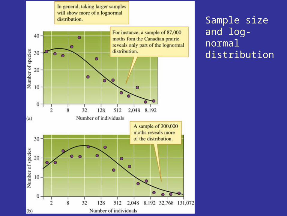
Sample size and log-normal distribution

How to explain the log-normal distribution of commonness and rarity?
May (1975) proposed that the log-normal distribution is the product of many random environmental variables acting upon the populations of many species. Relative abundances of large, heterogeneous assemblages of species governed by many independent factors will, according to the central limit theorem of statistics, be log-normally distributed.
True for any large heterogeneous collection, e.g. distribution of wealth in the USA and the distribution of the human population among the nations of the world.

Is the log-normal distribution just a mathematical artefact or does it reflect important biological processes?
May be a consequence of species within a community subdividing available niche space and of equilibrium or balance within community.
Very robust, may be the result of the law of large numbers or may be the result of biological processes.
Emphasises that few species are very abundant or extremely rare. Most species are moderately abundant.
Remarkably consistent and best described (though least understood!) pattern in community ecology.
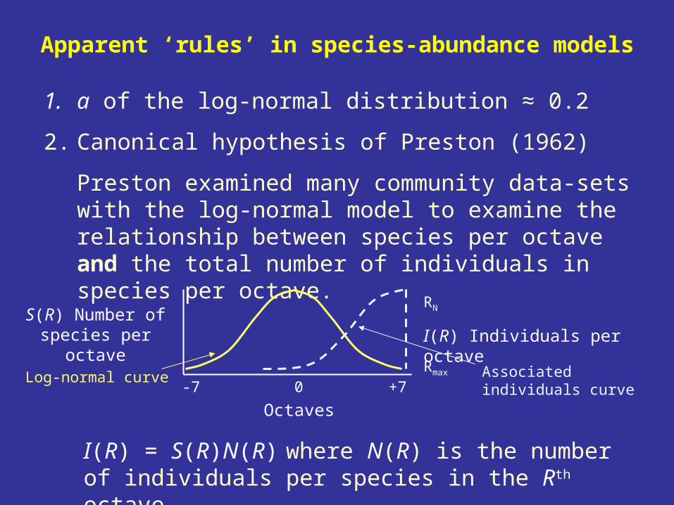
Apparent ‘rules’ in species-abundance models
1. a of the log-normal distribution ≈ 0.2
2. Canonical hypothesis of Preston (1962)
Preston examined many community data-sets with the log-normal model to examine the relationship between species per octave and the total number of individuals in species per octave.
S(R) Number of species per octave
Octaves-7 +70
RN
Rmax
I(R) Individuals per octave
I(R) = S(R)N(R) where N(R) is the number of individuals per species in the Rth octave
Log-normal curve Associated individuals curve
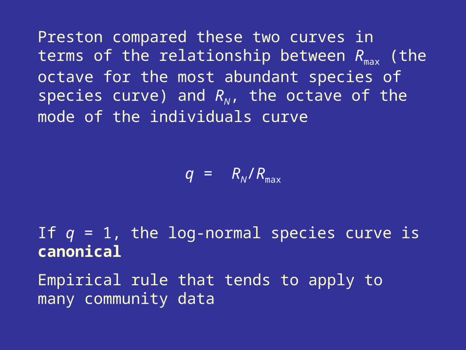
Preston compared these two curves in terms of the relationship between Rmax (the octave for the most abundant species of species curve) and RN, the octave of the mode of the individuals curve
q = RN/Rmax
If q = 1, the log-normal species curve is canonical
Empirical rule that tends to apply to many community data

Why should a be about 0.2 and q about 1?
May (1975) showed that the two ‘rules’ may be properties of the log-normal distribution.
1. General relationship between the total number of species and individuals, S and N, and parameters a and q
2. For values of S from 20-10000 and for N from 10S to 107S, parameter a lies in range 0.1-0.4 and q is 0.5-1.8
Are a and q therefore just statistical generalities associated with large samples?
Lord Bob May of Oxford
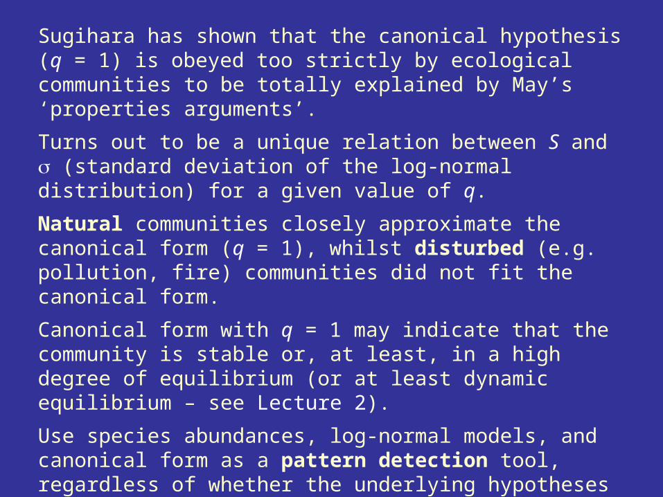
Sugihara has shown that the canonical hypothesis (q = 1) is obeyed too strictly by ecological communities to be totally explained by May’s ‘properties arguments’.
Turns out to be a unique relation between S and (standard deviation of the log-normal distribution) for a given value of q.
Natural communities closely approximate the canonical form (q = 1), whilst disturbed (e.g. pollution, fire) communities did not fit the canonical form.
Canonical form with q = 1 may indicate that the community is stable or, at least, in a high degree of equilibrium (or at least dynamic equilibrium – see Lecture 2).
Use species abundances, log-normal models, and canonical form as a pattern detection tool, regardless of whether the underlying hypotheses proposed for the model are correct or not.

Rank-Abundance Diagrams
Show distribution of all species abundances in a community for all m species present. Plot abundance pi for all i = 1,…,m species where pi is proportional abundance
Plot pi for the most abundant species first, then the next most common, and so on against species rank
Can be drawn for different communities or same community at different times
Grassland fertilised 1856-1949

Try to fit mathematical equations or ecological models to rank-abundance diagrams
Statistical models: log-series (LS)log-normal (LN)
Niche models: broken-stick (BS)geometric series (GS)
DD - dominance decayMF - MacArthur fractionRF - random fractionRA - random assortmentCM - composite DP - dominance pre-emption
For some explanation of these models, see Begon et al. (2006 pp. 472-473).

Species Numbers (= Richness) and Species Diversity
Species diversity consists of two components1. Number of species in community – 'species richness'2. Species evenness or equitability – how the species
abundances (e.g. cover, frequency) are distributed among the species.
Two communities1 - 10 species: 90% of individuals belong to species A;
10% of individuals belong to species B, C, D, E, F, G, H, I, J
2 - 10 species: 10% of individuals belong to each of species A-J
Community 1 has low evenness, 2 has maximum evenness

Richness indices
Evenness indices
Richness index + evenness index = Diversity index
Confound several properties of community structure, namely number of species; relative species abundance (evenness); and homogeneity and size of the area sampled.
Species identity not considered.

Richness indices
S – total number of species found in a community
But S depends on sample size and the time spent searching
Need to estimate S independent of sample size
But samples usually of different size
Rarefaction analysis – estimates how many species would be found in a sample of n individuals [denoted as E(Sn)] drawn from a population of N total individuals among S species.
s
i
in n
N
n
nNSE
1
1)(
where ni = number of individuals of species i

Rarefaction curves for three bird habitats showing expected numbers of species (E(Sn)) as a function of sample size
Three habitats 20 38 species (S), 122 birds (N)
9 14 species (S), 50 birds (N)
36 8 species (S), 62 birds (N)
How many species would be observed if all habitats had same sample size of 50 birds each?
E(Sn) habitat 20 26.9 species
9 14.1 species
36 7.8 species

Estimate of the total number of species S* (from the log-normal model) can also be used as a richness index.
Requires a statistical fit of the species abundances to the log-normal frequency distribution.
Computationally difficult, but not much more difficult than estimating E(Sn) in rarefaction analysis.

Evenness can be quantified by expressing Simpson’s index
(see below)
as a proportion of the maximum value possible when we assume that all individuals are completely evenly distributed amongst the species
Lowest value is 1: higher the value, greater the evenness. The maximum value is the total number of species;max = S. See below for more about evenness indices.
Thus, evenness E =
Evenness or ‘equitability’ indices
s
lip
1
2
11
Sp
s
li
11/1
1
2max

Combines species richness and evenness of relative abundance and compares richness and evenness of relative abundances between two or more samples
Diversity indices

Two forests, 5 species only but (b) has higher evenness
5 species; 84% A, 4% B, 4% C, 4% D, 4% E
5 species; A, B, C, D, & E each 20%
Forest (b) more diverse
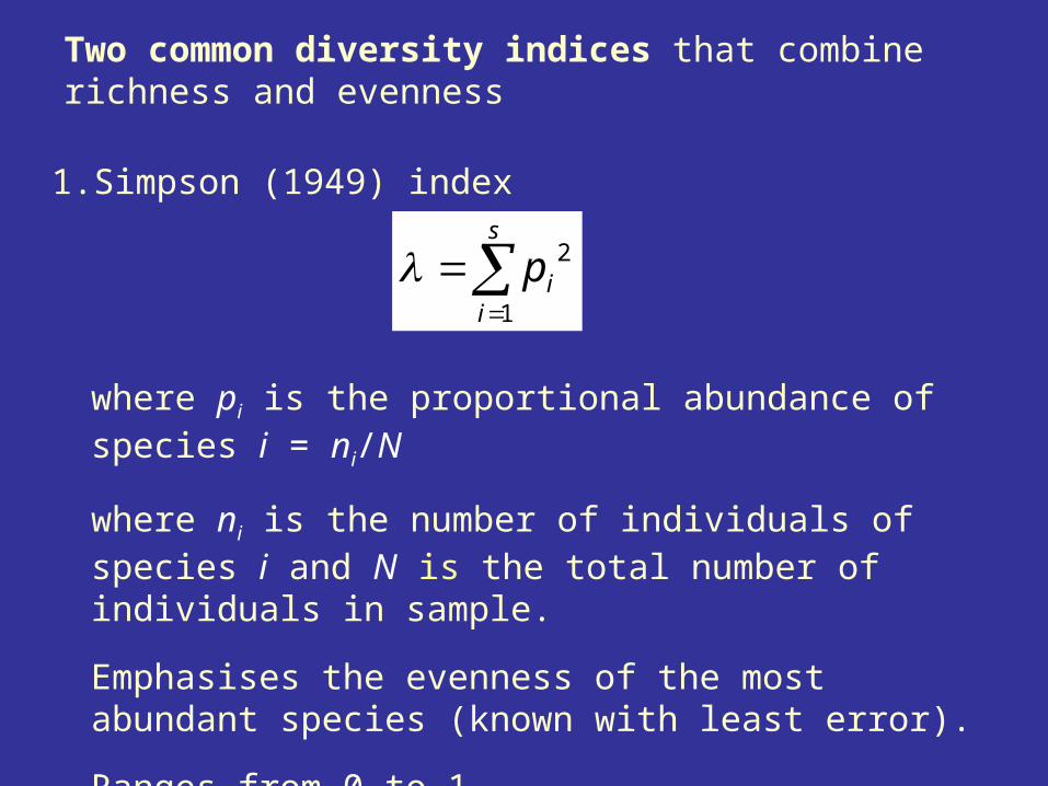
Two common diversity indices that combine richness and evenness
1. Simpson (1949) index
where pi is the proportional abundance of species i = ni/N
where ni is the number of individuals of species i and N is the total number of individuals in sample.
Emphasises the evenness of the most abundant species (known with least error).
Ranges from 0 to 1.
s
iip
1
2

As the greater the value of , the lower the diversity is, conventional to use
1 – as Simpson's index of diversity, D
Ranges between 0 and 1. In the absence of any diversity (only one species is present), the value of = 1 and D = 0.
D represents the probability that two individuals randomly selected from a sample will belong to different species.
Often used as 1/. Lowest value is 1; higher the value, greater the diversity. The maximum value in this case is the number of species in the community (species richness).
Important to know if using , 1 – , or 1/.

2. Shannon-Wiener index (H') (also known as Shannon-Weaver index)
Based on information theory and is a measure of the average degree of uncertainty in predicting what species an individual chosen at random from a collection of S species and N individuals will belong.
Average uncertainty increases as species number increases and as the distribution of individuals among the species becomes even.
Thus;
(1) H' = 0 if and only if there is one species present
(2) H' is maximum only when all S species are evenly distributed

s
iiei ppH
1
log'
where pi is the proportion of species i
loge is natural logarithm of pi
S is number of species
Simply determine proportions of each species, pi, and the loge of pi. Multiply each pi times loge
pi, and sum the results for all species from 1 to
S. As the sum will be negative, H' is the opposite sign.

Evenness
where H’ is Shannon-Wiener diversity index, S is number of species, and Hmax = logeS
S
pp
H
HJ
e
s
iiei
log
log' 1
max

Two forests, 5 species only but (b) has higher evenness
5 species: 84% A, 4% B, 4% C, 4% D, 4% E H' = 0.662
5 species: A, B, C, D, & E each 20% H' = 1.610
Forest (b) more diverse
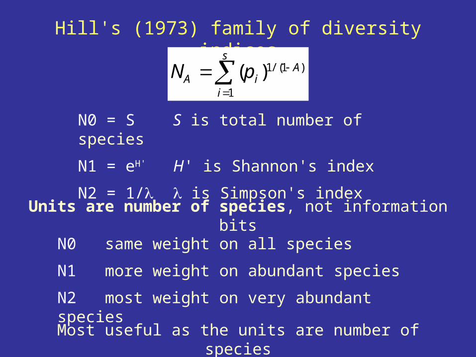
Hill's (1973) family of diversity indices
N0 = S S is total number of species
N1 = eH' H' is Shannon's index
N2 = 1/ is Simpson's index
Units are number of species, not information bits
N0 same weight on all species
N1 more weight on abundant species
N2 most weight on very abundant species
Most useful as the units are number of species
s
i
AiA pN
1
)1/(1)(
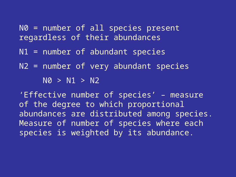
N0 = number of all species present regardless of their abundances
N1 = number of abundant species
N2 = number of very abundant species
N0 > N1 > N2
‘Effective number of species’ – measure of the degree to which proportional abundances are distributed among species. Measure of number of species where each species is weighted by its abundance.

N0, N1, and N2 differ only in their tendency to include or ignore rare species
11 species
abundances are 90, 1, 1, 1, 1, 1, 1, 1, 1, 1, 1
N2 = 1.23
N1 = 1.74
N0 = 11
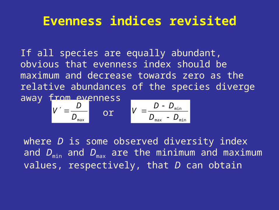
Evenness indices revisited
maxDD
V
If all species are equally abundant, obvious that evenness index should be maximum and decrease towards zero as the relative abundances of the species diverge away from evenness
orminmax
min
DDDD
V
where D is some observed diversity index and Dmin and Dmax are the minimum and maximum values, respectively, that D can obtain
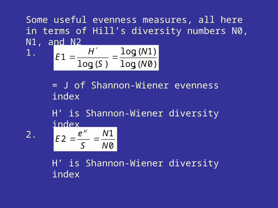
Some useful evenness measures, all here in terms of Hill’s diversity numbers N0, N1, and N2
)0(log)1(log
)(log1
NN
SH
En
n
n
= J of Shannon-Wiener evenness index
H’ is Shannon-Wiener diversity index
1.
2.01
2NN
Se
EH
H’ is Shannon-Wiener diversity index

3.
1011
11
3
NN
Se
EH
4.121
4NN
eE
H
5.1112
111
5
N
Ne
EH
Hill ratio
Modified Hill ratio
This approaches zero as a single species becomes more and more dominant, unlike E4 which approaches 1
E5 is preferred evenness index

Evenness index should be independent of number of species in the sample
E1 (= J) strongly affected by species richness
E2 and E3 also strongly sensitive to richness
E4 and E5 unaffected by richness. Best to use.
Species Abundances E1 E2 E3 E4 E5
3 500, 300, 200 0.94 0.93 0.90 0.94 0.91
4 500, 299, 200, 1 0.75 0.71 0.61 0.94 0.90
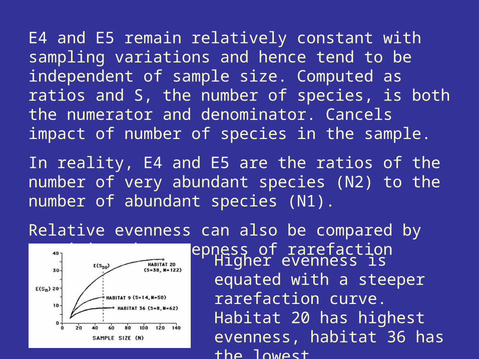
E4 and E5 remain relatively constant with sampling variations and hence tend to be independent of sample size. Computed as ratios and S, the number of species, is both the numerator and denominator. Cancels impact of number of species in the sample.
In reality, E4 and E5 are the ratios of the number of very abundant species (N2) to the number of abundant species (N1).
Relative evenness can also be compared by examining the steepness of rarefaction curves.
Higher evenness is equated with a steeper rarefaction curve. Habitat 20 has highest evenness, habitat 36 has the lowest.
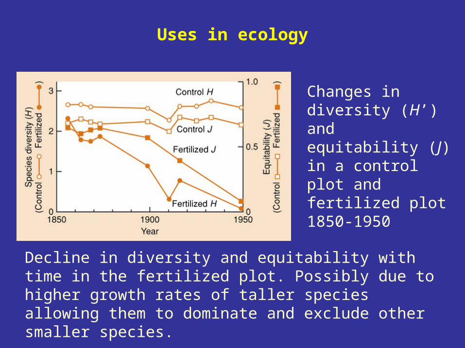
Uses in ecology
Changes in diversity (H’) and equitability (J) in a control plot and fertilized plot 1850-1950
Decline in diversity and equitability with time in the fertilized plot. Possibly due to higher growth rates of taller species allowing them to dominate and exclude other smaller species.

Not all Species are Equal!
In a functional role, not all species in a community appear to be equal.
1. Few common species with a high population density or relative abundance. Called dominants.
Dominance is the converse of diversity. Simpson's is often used as a measure of dominance. A value of 1 would represent total dominance (only one species present).
Dominance may not be numerical abundance but may be biomass, functional importance, or size of the individuals.
2. Many rare species with a low population density or relative abundance. Called rarities.

3. Keystone species – may be less abundant but play a crucial role in the function of the community.
Keystone species have a unique and significant role through their activities and their overall effect on the community may not be related or proportional to their abundance.
If removed, major changes in community structure occur along with a significant loss of diversity.
Role of keystone species may be to create or modify habitats or to influence the interactions between other species.

Examples of keystone species are
1. Herbivores e.g. African elephant in savanna communities
2. Predators e.g. sea otters (Enhydra lutris) eat sea-urchins in kelp sea-weed beds. Kelp beds provide habitats for many other species. If sea otters decline, sea-urchin populations increase resulting in overgrazing of kelp beds and loss of habitat for many species.
3. Coral Oculine arbuscula – more than 300 invertebrate species live among its branches.

Keystone species are like pieces in a Jenga game
In a game of Jenga, players successively take away parts and place them on top until the structure becomes unstable and crashes. Each part can thus be a keystone. When parts are replaced at other positions, the stability of the Jenga structure can be maintained.
Keystone species may be like pieces in a Jenga game. But we do not really know. Very difficult to find out.
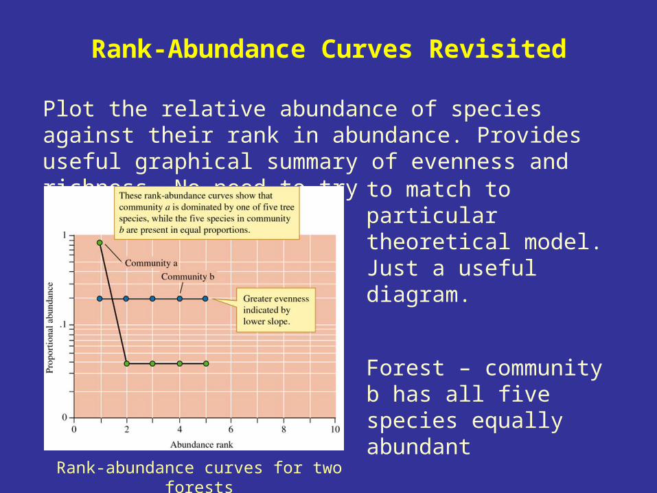
Rank-Abundance Curves Revisited
Plot the relative abundance of species against their rank in abundance. Provides useful graphical summary of evenness and richness. No need to try
Rank-abundance curves for two forests
Forest – community b has all five species equally abundant
to match to particular theoretical model. Just a useful diagram.
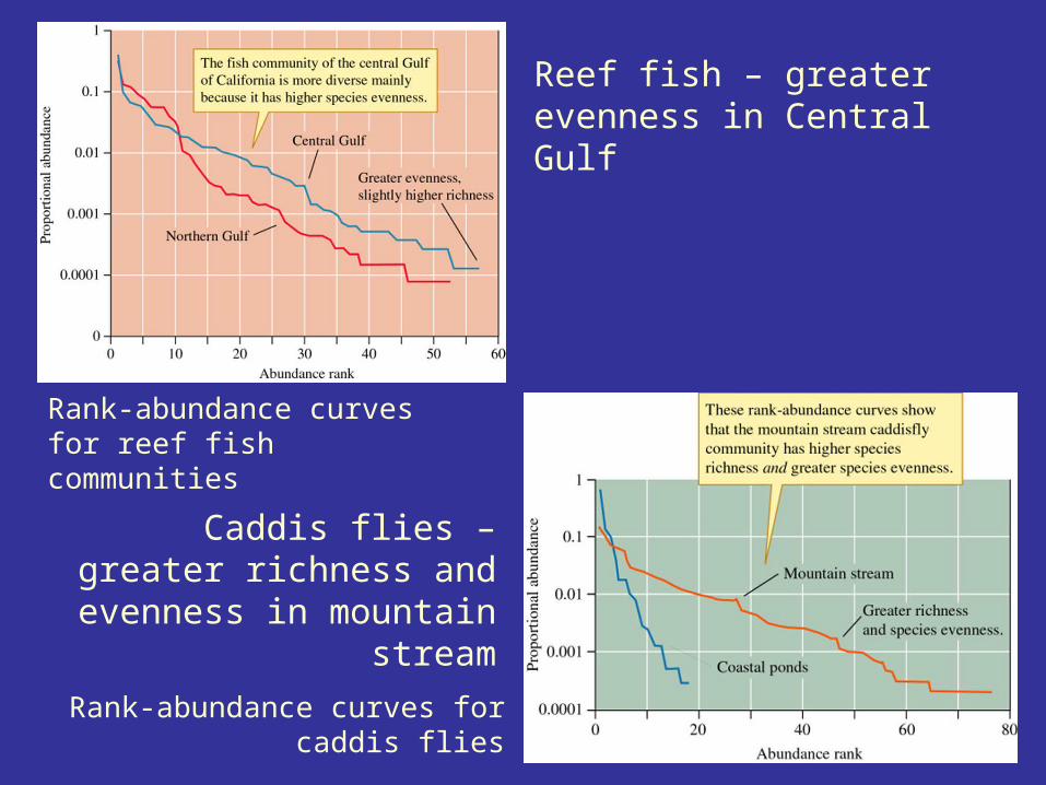
Rank-abundance curves for caddis flies
Rank-abundance curves for reef fish communities
Reef fish – greater evenness in Central Gulf
Caddis flies – greater richness and evenness
in mountain stream

What Determines Diversity?
High biodiversity is often associated with high eco-complexity or environmental complexity.
In general species diversity increases with environmental complexity or heterogeneity.
But one aspect of the environment may be important to one group of organisms but may not be important to another group.
Need to know something about the ecological requirements of species (niches) to predict how environment influences their diversity.

Environmental Complexity
1. Forest complexity and bird species diversity
Competition influences species realised niches.
Competitive exclusion principle predicts that co-existing species will have different realised niches.
Warblers (sangere) in eastern USA forests
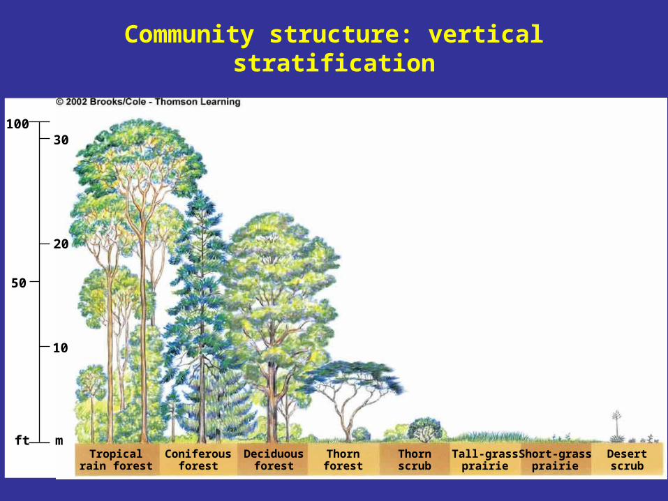
mft
10
50
20
30100
Tropicalrain forest
Coniferousforest
Deciduousforest
Thornforest
Tall-grassprairie
Short-grassprairie
Desertscrub
Thornscrub
Community structure: vertical stratification

Forest community structure
Emergent
Canopy
Understorey
Floor
Subsoil
Birds, invertebrates,bats
Birds, reptiles,amphibians,lichens, mosses
Shade-tolerant plants, birds, squirrels,lizards, chipmunks
Rotting debris,worms, insects,bacteria
Nematodes,micro-organisms
Bole
Snag

Five different warblers (sangere)
Essential to study community structure to provide basis for explaining co-existence of different species of same genus in forests

Species forage in different layers in forest.
Distributions may be influenced by vertical structure of vegetation.
Mount Desert Island, Maine
Robert McArthur measured relationship between volume of vegetation above 6 m and warbler abundance

Stature of vegetation and no. of warbler species
Warbler diversity increased as stature of vegetation increased
i.e. species diversity increased with habitat size.
What about habitat diversity?
Estimated forest habitat diversity by Shannon-Wiener index.

Foliage height and bird species diversity

In absence of black-throated green warbler, the yellow-rumped warbler expands its range
Structure PLUS between-species interactions are important

General (but not universal!) pattern that species diversity (biodiversity) increases with environmental complexity (eco-complexity) or habitat diversity.
mammals lizards reptiles reef fish birds marine gastropods
What about plants?

2. Niches of algae and terrestrial plants
At least 270,000 species of terrestrial plantsProvides great scope for animal niche specialisation
But how can we explain the diversity of primary producers?
"The paradox of the plankton" G.E. Hutchinson (1961)
Paradox because plankton live in relatively simple environments (open water of lakes and oceans) and compete for N, P, Si, etc. and yet many species co-exist without competitive exclusion.
Same for terrestrial plants – how can they co-exist?
Need to understand the nature of their niches.
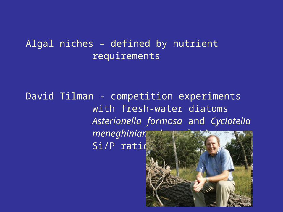
Algal niches – defined by nutrient requirements
David Tilman - competition experiments with fresh-water diatoms Asterionella formosa and Cyclotella meneghiniana in relation to Si/P ratio

Ratio of silicate to phosphate
High Si/P ratios, Asterionella dominant in P limited situations. Takes up P faster, depletes environment of P, eliminates Cyclotella.
Low Si/P ratios, Cyclotella dominant as Si limits growth of Asterionella and so Asterionella cannot deplete the P and eliminate Cyclotella.
When both Si and P are limiting (medium ratios) two species can co-exist.
Two planktonic species can co-exist in a lake because of spatial variation in P and Si values.

Niches of plants and algae largely defined on basis of nutrient requirements (e.g. N, P, K, Si) and responses to physical or chemical conditions (e.g. temperature, soil pH, moisture).
Thus environmental variation in availability of nutrients, temperature, moisture, pH, etc. creates the environmental complexity required for plant species co-existence.

Concentrations of nitrate and silicate in Pyramid Lake, Nevada
Aquatic environment
Spatial variations in NO3 and SiO2 (also phosphate and chlorophyll a) create a wide range of environ-mental complexity

Terrestrial environment
0.5 ha plot (69 m x 69 m) 301 sampling points Measured soil moisture and soil NO3 in an abandoned agricultural field in Michigan.
Shows considerable spatial variability within a small area.
How does this spatial heterogeneity in essential resources influence plant distribution and diversity?
10-fold difference across study plot
No correlation between the two variables

Amazon forest – one of the most complex vegetation types known.
Jordan (1985) showed
(1) large numbers of species live within most tropical plant communities, and
(2) there are a large number of plant communities in a given area.
There is thus a high alpha-diversity (diversity within habitat or community) and high beta-diversity (between habitat or community diversity).
There is also high gamma-diversity (rich 'species-pool') due to historical reasons.

Small differences in soil properties result in different plant communities. Six types in 2500m over an elevational range of less than 8 m.
Granite bedrock, clay subsoil, varying amounts of sand, small variations in topography determining depth of the soil above the groundwater.

Communities - Hill tops, shallow sand 'Mixed'
- Thicker sand 'Yévaro'
- Stream edges & floodplain
'Igapó'
- Above flooding level 'Caatinga'
- 1.2 m above stream level
'Campina'
- >2 m above stream level
'Bana'
All in 2500 m and 8 m elevational range
Subtle changes in physical and chemical environment gives high eco-complexity and hence high biodiversity

3. Role of increased nutrient availability and enrichment
Generally there is a negative relationship between diversity and nutrient availability.
As nutrients increase, species diversity decreases.
Soil fertility and plant species in Ghana forests

Park Grass Experiment, England since 1856
Shows decline in diversity on plots that have been fertilized by N, P, and K from 49 species to 3 species
Control plots – no change.
Fertilization and plant diversity
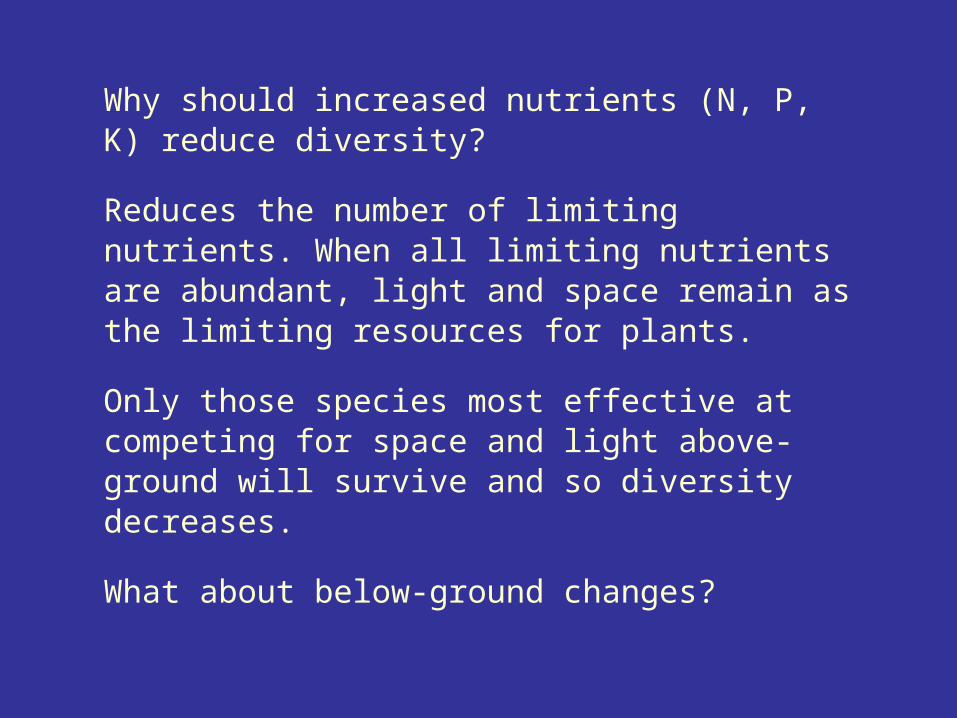
Why should increased nutrients (N, P, K) reduce diversity?
Reduces the number of limiting nutrients. When all limiting nutrients are abundant, light and space remain as the limiting resources for plants.
Only those species most effective at competing for space and light above-ground will survive and so diversity decreases.
What about below-ground changes?

Ectomycorrhizal fungal diversity along a soil nitrogen gradient downwind from a fertilizer plant on Kenai Peninsula, Alaska
Gradient from 13.3 mg kg-1 to 243 mg kg-1 extractable NO3
Looked at ectomycorrhiza on roots of Picea glauca (white spruce) trees.

Relationship between soil nitrogen and ectomycorrhizal
community diversity
Clear decline in mycorrhizal diversity with increase in soil nitrogen.
Possibly a change from species specialised for nitrogen uptake under conditions of low available N to small number of fungi associated with unusually high soil fertility.

Environmental diversity (eco-complexity) can certainly account for much of the observed patterns in diversity.
What about the role of disturbance on diversity?

Disturbance and Diversity
Ecologists tend to assume environmental conditions remain more or less stable. Equilibrium
Lotka-Volterra competition models and predator-prey models assume a constant physical environment.
But the physical environment varies continuously in space and time at all scales. As a result, the biotic environment will also vary, as will the frequency and intensity of disturbance. Non-equilibrium
Disturbances often occur when there is a rapid shift from 'average' conditions (e.g. storms).
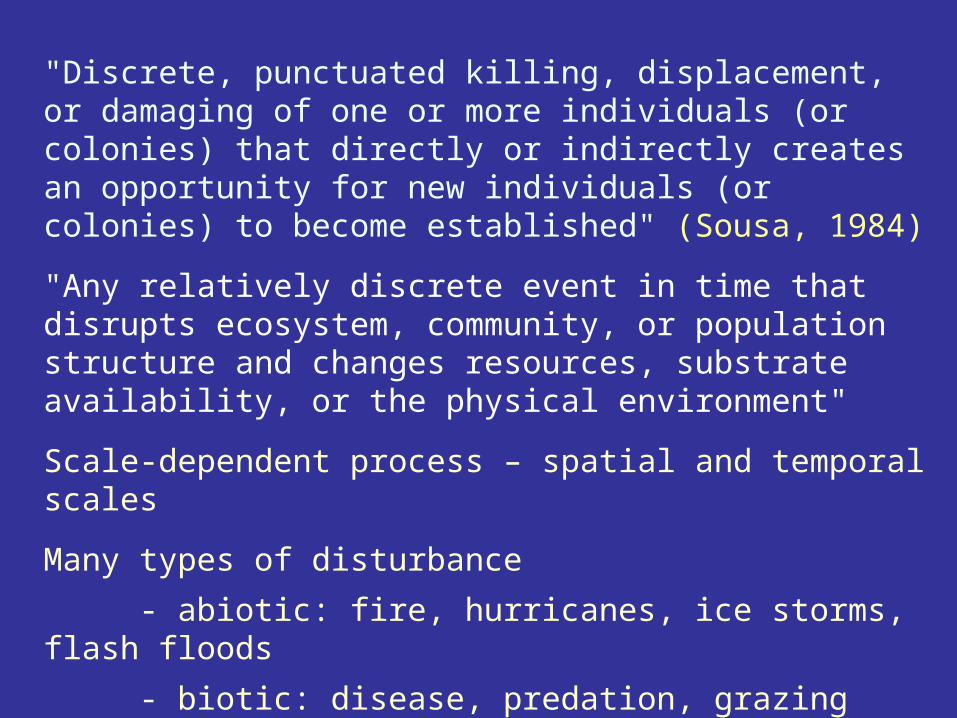
"Discrete, punctuated killing, displacement, or damaging of one or more individuals (or colonies) that directly or indirectly creates an opportunity for new individuals (or colonies) to become established" (Sousa, 1984)
"Any relatively discrete event in time that disrupts ecosystem, community, or population structure and changes resources, substrate availability, or the physical environment"
Scale-dependent process – spatial and temporal scales
Many types of disturbance
- abiotic: fire, hurricanes, ice storms, flash floods
- biotic: disease, predation, grazing
- human: forest clearance

As all communities experience disturbance and as environment is never stable, proposed that diversity is a result of changing conditions and not competitive accommodation at equilibrium.
Predicts that intermediate levels of disturbance promote higher levels of diversity.
Joseph Connell
'intermediate disturbance hypothesis'

Intermediate disturbance hypothesis

Intense and/or frequent disturbance – only a few species able to colonise and complete their life cycles between the frequent disturbances.
Mild and/or infrequent disturbance – only a few species are strong competitors at using available resources or most effective at interference competition.
At intermediate levels of disturbance, there is sufficient time between disturbances for many species to colonise but not long enough for competitive exclusion.

1. Intertidal zone (Sousa 1979)
Algae and invertebrates growing on boulders. Small boulders more likely to be disturbed by waves and storms than large boulders.
Estimated wave force needed to move boulders
3 types - frequent movement (42% per month)
intermediate movement (9% per month)
infrequent movement (1% per month)
Number of species recorded

Levels of disturbance and diversity on intertidal boulders
2 species on low-disturbance boulders
4 species on intermediate-disturbance boulders
1 species on high-disturbance boulders
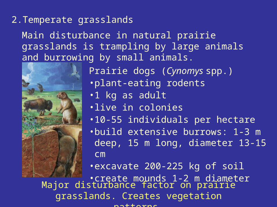
2. Temperate grasslands
Main disturbance in natural prairie grasslands is trampling by large animals and burrowing by small animals.
Prairie dogs (Cynomys spp.)•plant-eating rodents •1 kg as adult •live in colonies•10-55 individuals per hectare•build extensive burrows: 1-3 m deep, 15 m long, diameter 13-15 cm
•excavate 200-225 kg of soil•create mounds 1-2 m diameter
Major disturbance factor on prairie grasslands. Creates vegetation patterns.
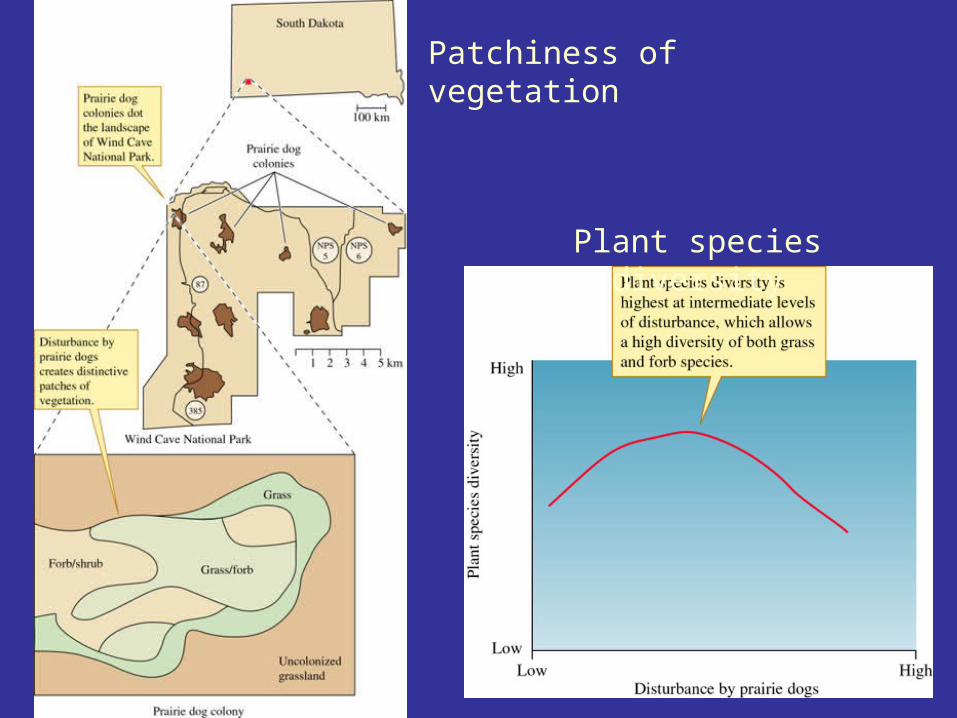
Patchiness of vegetation
Plant species diversity

Too much disturbance – only a few colonisers can grow
Too little disturbance – only the major competitors can grow
However, prairie dogs are thought of as an agricultural pest and populations have fallen by 98% in last century.
Pocket gophers have similar ecological role as prairie dogs and maintain species diversity in prairie grasslands.

3. Human disturbance
Tend to think of Panamanian rain forests as undisturbed ecosystems and yet they have high diversity. How is this possible? Are they disturbed?
Palaeoecology – examine pollen and spores preserved in lake sediments covering the last 3000-5000 years (Lecture 5).
Lake Wodehouse, Panama

Pollen and charcoal

1. Charcoal and Zea (corn) appear 3900 years ago
2. Prior to that time, was a swamp with mature tropical forest
3. Charcoal and Zea disappear 310 years ago
4. Forest species increase in abundance
Appears here and elsewhere in tropics, that low-intensity human disturbance involving slash-and-burn cultivation has been occurring for last 5000-11000 years.
Low-intensity human disturbance may be an integral part of rain forest system (and many other systems).
Contrasts with massive clear-cutting of Amazonian rain forest today. Results in much reduced diversity.

4. European calcareous grasslands
Very species-rich communities – 50 species m-2
High diversity is maintained by moderate levels of human disturbance.
Grasslands created by humans and forest clearance. Used for livestock grazing and harvesting hay for winter fodder.
Grazing and mowing resulted in high plant diversity.
When traditional land-use was abandoned, diversity decreased and monoculture of the grass Brachypodium pinnatum developed.

Species-rich grassland, Pewsey
Brachypodium pinnatum turf,
Barnock Hills

Changes in plant species coverage

Bobbink & Willems (1991) working in Limburg, SE Holland, investigated if they could reverse the declines in diversity by using traditional autumn mowing.
Tried autumn and summer mowing 1982 – 1986.
Brachypodiumpinnatum Richness
Summer 77 34% 15.6 21.2
Autumn 75 80% 7.2 7.8
Why the difference between summer and traditional autumn mowing?

Investigated
(1) autumn mowing
(2) late summer mowing
(3) early summer mowing
(4) early summer + autumn mowing
Only mowings (2) and (4) diminish the Brachypodium pinnatum by reducing carbohydrates in the rhizomes that are important for shoot formation. By reducing the carbohydrates and shoot formation, reduce the competitive ability of Brachypodium.
But why is the traditional autumn mowing no longer sufficient to maintain the original high diversity of this grassland?

Recent human activity has altered the nitrogen cycle, increased the atmospheric N content, and increased the soil N.
Increased soil N appears to strongly favour Brachypodium.
Another example of increasing nutrient availability reducing plant diversity by favouring those species that are the most effective competitors for the remaining resources.
Shows complex relationships within communities and the determinants of diversity.

What Determines Community Structure?
Most fundamental process in nature is acquiring food or energy and nutrients needed for assimilation.
Species interactions of predation, parasitism, competition, and mutualism all important in obtaining resources.
Food chain
Grass Insect Bird Bird of prey

Food chains never this simple. Numerous chains fused or meshed into a complex food-web with complex links leading from primary producers to consumers.

P – top predator, not eaten by other species in food-web
C1, C2, - intermediate species, C1 is an omnivore, C2 is a carnivore
H1, H2, H3 – intermediate species, herbivores
A1 and A2 – basal species, primary producers
Hypothetical food-web

Real-life food-web for Tuesday Lake, Michigan, USA
de Ruiter et al. (2005)

How do species co-evolve and shape complex webs of mutualistic interactions? Part of community structure
Plants and free-living pollinators and seed-dispersal agents. Most visible, diverse, and mutualistic interactions. Involves dozens or even hundreds of plant and animal species.
Do these mutualistic interactions lead to a predictive pattern of links between species?
Using network theory, can show that specialisation (bees only visiting flowers of 1 or 2 species) withinthe web is nested. In a nested web, there is a core group of generalists that interact with each other and extreme specialists that interact only with generalist species.

Result is a web with many asymmetries in degree of specialisation among interacting species. In contrast, interactions between predators and prey or herbivores and plants are often in compartments and form small clusters within the broader interaction web.
Studies in montane forest in SE Spain, Bascompte et al. (2006 Science 312: 431) show that the distribution of specialists and generalists within these webs is unlikely to be due to chance.
Asymmetries in specialisation between pairs of interacting species are the rule.

Plant might rely heavily on seed-dispersal by a particular seed-eating (frugivore) species, but the same frugivore might consume fruits from many plant species.
Assymmetry in specialisation promotes species coexistence within these interactions over evolutionary time.

Complex mutualistic webs are not haphazard collections of specialists and generalists
Evolution and co-evolution appear to shape these interactions in a predictable way regardless of the exact species composition
An important part of community structure is the role of mutualistic interactions
Perhaps there will, one day, be a theory of co-evolution and community structure
We are a long way from any such theory!
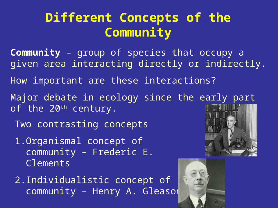
Different Concepts of the Community
Community – group of species that occupy a given area interacting directly or indirectly.
How important are these interactions?
Major debate in ecology since the early part of the 20th century.
Two contrasting concepts
1. Organismal concept of community – Frederic E. Clements
2. Individualistic concept of community – Henry A. Gleason

1. Organismal concept of community – each species represents an interacting, integrated component of the whole.

Species have similar distributions along an environmental gradient. May peak at same point.
Transition between associations (communities) are narrow.
Suggests a common history and similar fundamental niches (responses and tolerances). Mutualism and co-evolution are important in the evolution of species in the community.
Community is thus an integrated whole; the species interactions are the "glue" that holds it all together.
Discrete units, plant associations, alliances, etc.
Plant ecology, classification, phytosociology.

2. Individualistic concept of community – relationships between co-existing species are a result of similarities in their requirements at that one point in space and are not a result of strong interactions or common history.

Gleason proposed that species abundances change so gradually along gradients that it is not practical to divide the vegetation into associations. Species distributions do not form clusters but represent independent or individualistic responses of species. Transitions are gradual and difficult (or impossible!) to identify.
Community here is merely the group of species found to co-exist under a particular set of environmental conditions.
Species distributed as a continuum in response to variation in the environment in space and time.
Gradient analysis and ordination.

Models of taxa along gradients
Kent & Coker (1992)
Community concept
Individualistic concept
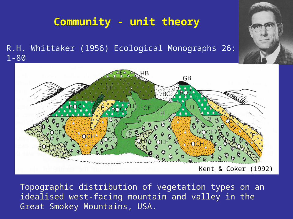
Community - unit theory
R.H. Whittaker (1956) Ecological Monographs 26: 1-80
Kent & Coker (1992)
Topographic distribution of vegetation types on an idealised west-facing mountain and valley in the Great Smokey Mountains, USA.

Community - unit - vegetation of an area is distributed as a mosaic, so-called climax pattern.
Broadly similar environmental factors (both abiotic and biotic) occur and repeat themselves in an area. Not all areas can be placed in one or other type. Boundaries may be distinct or vague (ecotones).
60 - 80% can be unambiguously assigned to particular vegetation types.
20 - 40% can not be assigned because they are transitional or ecotonal areas between types.
Community - unit vegetation - landform unit. Features of landscape.
Noda - reference points in a continuum of either geographical or environmental space.
Continuum of species responses in environmental space or gradients. Features of underlying environment.

Major differences between these two concepts are the relative importance of interactions, evolutionary history, and co-evolution in determining community structure.
Evidence for both concepts – the natural world shows both discontinuous (organismal concept) and continuous (individualistic concept) change at different spatial and temporal scales).
Testing of these competing concepts and hypotheses requires knowledge about community history and development through time. Lecture 2 on Community Ecology and Dynamics.

Gradients and landscapes
Patterns of co-occurrence of four species on a landscape along an indirect environmental gradient altitude; note continuous variation of composition along altitude gradient. A plant community is a landscape concept and recognition of communities depends on the frequency of environmental combinations in a particular landscape.
Austin & Smith (1989)

Important distinction between geographical distribution and environmental distribution.
In geographical space, have species associations A, AB, B, C, and D with BC and CD as 'ecotones'. These associations are a consequence of the spatial pattern of the landscape.
In environmental space, find a continuum of species A, B, C, and D replacing each other with increasing altitude.
Communities or associations are a function of the landscape examined.
Continuum concept applies to the environmental space, and not necessarily to geographical distance on the ground or to any indirect or complex environmental gradient.
Community concept and continuum concept not alternatives but are features of vegetation viewed in different ways - geographical space or environmental space.

How to Analyse Community-Scale Data?
Classification and gradient analysis (= ordination)Simple example - European food
GC ground coffee 90 82 88 96 94 97 27 72 55 73 97 96 96 98 70 13IC instant coffee 49 10 42 62 38 61 86 26 31 72 13 17 17 12 40 52TB tea or tea bags 88 60 63 98 48 86 99 77 61 85 93 92 83 84 40 99SS sugarless sugar 19 2 4 32 11 28 22 2 15 25 31 35 13 20 - 11BP packaged biscuits 57 55 76 62 74 79 91 22 29 31 - 66 62 64 62 80SP soup (packages) 51 41 53 67 37 73 55 34 33 69 43 32 51 27 43 75ST soup (tinned) 19 3 11 43 25 12 76 1 1 10 43 32 4 10 2 18IP instant potatoes 21 2 23 7 9 7 17 5 5 17 39 11 17 8 14 2FF frozen fish 27 4 11 14 13 26 20 20 15 19 54 51 30 18 23 5VF frozen vegetables 21 2 5 14 12 23 24 3 11 15 45 42 15 12 7 3AF fresh apples 81 67 87 83 76 85 76 22 49 79 56 81 61 50 59 57OF fresh oranges 75 71 84 89 76 94 68 51 42 70 78 72 72 57 77 52FT tinned fruit 44 9 40 61 42 83 89 8 14 46 53 50 34 22 30 46JS jam (shop) 71 46 45 81 57 20 91 16 41 61 75 64 51 37 38 89CG garlic clove 22 80 88 16 29 91 11 89 51 64 9 11 11 15 86 5BR butter 91 66 94 31 84 94 95 65 51 82 68 92 63 96 44 97ME margarine 85 24 47 97 80 94 94 78 72 48 32 91 94 94 51 25OO olive, corn oil 74 94 36 13 83 84 57 92 28 61 48 30 28 17 91 31YT yoghurt 30 5 57 53 20 31 11 6 13 48 2 11 2 - 16 3CD crispbread 26 18 3 15 5 24 28 9 11 30 93 34 62 64 13 9
D I F NL B L GB P A CH S DK N SF E IRL
(from A Survey of Europe Today, The Reader’s Digest Association Ltd.) % of all households with various foods in house at time of questionnaire. Foods by countries.
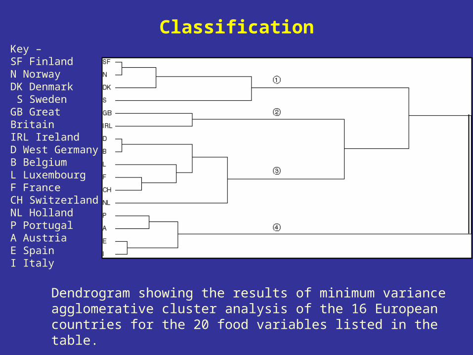
Classification
Dendrogram showing the results of minimum variance agglomerative cluster analysis of the 16 European countries for the 20 food variables listed in the table.
Key – SF Finland N Norway DK Denmark S Sweden GB Great Britain IRL Ireland D West Germany B Belgium L Luxembourg F France CH Switzerland NL Holland P Portugal A AustriaE Spain I Italy
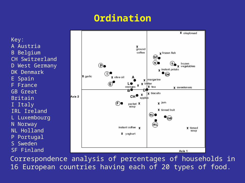
Ordination
Correspondence analysis of percentages of households in 16 European countries having each of 20 types of food.
Key: A Austria B BelgiumCH Switzerland D West Germany DK DenmarkE Spain F France GB Great Britain I ItalyIRL IrelandL Luxembourg N Norway NL HollandP Portugal S SwedenSF Finland

Classification and/or Ordination
Traditionally classification associated with the discontinuum or community concept of vegetation and ordination with the continuum concept.
Reflects the history of the methods but is the distinction valid?
Approaches are complementary: choice depends on the aim of the study.
Vegetation mapping - classification is necessary.
Fine-scale studies - ordinations are necessary to find repeatable patterns and discontinuities in composition.
Not a case of Classification or Ordination, but Classification and/or Ordination.

Diversity Components at Community Scale
R.H. Whittaker suggested several concepts of diversity:: diversity on a sample plot, or 'point' diversity (or within-habitat
diversity). Community: diversity along ecological gradients (or between-habitat diversity).
Differentiation diversity. Many meanings - poorly understood. Cannot be estimated unless there are known environmental gradients or the underlying latent structure of the data has been recovered. Between-community
: diversity among parallel gradients or classes of environmental variables. Product of -diversity of communities and -differentiation among them. Landscape
: diversity between landscapes. Differentiation diversity between landscapes. Between-landscape
ε: the total regional diversity of an area: sum of all previous components. Applicable to broad biogeographical areas. 'Species pool'. Regional
In practice, and diversities are rarely distinguished. ε is often used to designate the total diversity of a landscape, geographical area, or island. Incorrectly called diversity.

Ecologists recognise many types of diversity
•community (-diversity)
•between community (-diversity)
•landscape (-diversity)
•between landscapes (-diversity)
•regions (-diversity)
Odgaard 2007

Conclusions and Summary
1. Community is a collection of plants and animal populations found in one habitat type in one area and integrated to a degree by competition, complementarity, and dependence.
2. Species occur together because of the niches available in that habitat type.
3. Communities are most commonly recognised by their habitat type or the largest or most abundant species.
4. Communities are very complex and many questions arise:
- What is the community structure?
- What species are present?
- How many species are present?
- What are the abundance patterns of the species?
- How does the community function?
- What is the influence of the abiotic environment on the community?
- How does the community regenerate and sustain itself?
- What is its history?

5. Animal ecologists focus on guilds – organisms that function together. Plant ecologists may focus on life-forms or functional types.
6. Species abundance patterns usually follow the log-normal distribution, with few very abundant or very rare species, and many medium abundance species.
7. Log-normal distribution may just be a mathematical artefact and a result of the law of large numbers or it may be a result of biological processes.
8. Species diversity consists of species richness and species evenness.
9. Species richness depends on sample size and can be standardised by rarefaction analysis.

10. Two common diversity indices are the Simpson index and the Shannon-Wiener index. Simpson considers the evenness of the very abundant species, Shannon-Wiener considers the abundant species. Hill’s diversity numbers are very useful summaries and combine richness and evenness.
11. Rank-abundance curves display evenness and diversity graphically.
12. Species diversity is higher in complex heterogeneous environments.
13. High nutrient levels correlate with reduced diversity of algae, plants, and fungi.
14. Intermediate levels of disturbance promote higher diversity.

15. Human activity is an ancient feature of the bio-sphere and has provided intermediate disturbances for long periods of time.
16. Recent intensive human activity (widespread forest destruction, atmospheric N pollution) is decreasing community diversity.
17. Food acquisition, food chains, and food-webs are potential factors in determining community structure.
18. There are two major contrasting concepts of community organisation. Organismal and Individualistic concepts. Real world is a complex mixture of both.
19. Classification and ordination are both useful and valid approaches in analysing community data.

20. Besides -diversity of a sample plot or community, there is -diversity (between-habitat or between-community diversity), -diversity (landscape diversity, product of and -diversity), -diversity (between landscape), and (regional diversity).
21. Community ecology is the study of the community level of organisation, rather than the study of clearly definable spatial and temporal units. It is concerned with the structure and function of multi-species assemblages, usually, but not always, at one point in space and time.
22. It is not necessary to have sharp discrete boundaries between communities to study community ecology.

Ecological and Environmental Change Research Group (EECRG)
One of the largest research groups in the Department of Biology
Active in plant and animal ecological research, publication, teaching, supervision of PhD and MSc students, and studies in developing countries
MSc research in Norway, Svalbard, Tibet, Nepal, and Uganda
Many MSc topics relate to Lectures 1, 2, 5, 7-10
Colloquia for this part of Bio-201 led by Tessa Bargmann, an EECRG member
For further details, see www.eecrg.uib.no

EECRG Research Topics in this Lecture
Disturbance and diversity in several communities in Norway, Nepal, Svalbard, and Scotland
Diversity studies in several vegetation types in several countries
Ordination and gradient analysis of vegetation and faunal assemblages
Relationships between , and diversity (additive or multiplicative)
www.eecrg.uib.no


