Ecology of the Southwest-Lab #1faculty.fortlewis.edu/korb_j/Plant Community Ecology 2010... · Web...

Plant Community Ecology Course Packet, BIO 410Fall 2012

Dr. Julie Korb2445 Berndt Hall

[email protected]

Tuesday/Thursday 12:45-2:05 pm 310 Berndt Hall

TABLE OF CONTENTSDescription Page #'s

Syllabus 3-5Class Schedule 6-8Article Discussion Guidelines 9

In-Class Activities:Intro to Plant Ecology Worksheet 10-11Article Discussion Questions Week 1 12-13Releve Field Methods 14-17Animas Mountain Species List 18-20Quantifying Patterns Worksheet 21Article Discussion Questions Week 2 22-23PC-Ord Instruction Manual 24-44Life History Traits Worksheet 45-46Plant Intraspecific Competition Greenhouse Exercise 47-54Plant Interaction Worksheet 55-57Exam 1 Study Guide 58-60Fire 101 Worksheet 61-62Pinyon-Juniper Worksheet 63-64Mixed Conifer Worksheet 65-66Subalpine Worksheet 67-69PC-Ord Report Guideline 70-78Exam 2 Study Guide 79-80

2

BIO 410: Plant Community Ecology Fort Lewis College-Fall 2012

Class Schedule: T/R 12:45-2:05 p.m. Rm# Berndt 310

Instructor: Julie Korb, Ph.D. [email protected]: 2445 Berndt Hall phone: 382-6905Office Hours: T/R 2:05- 3:00 pm or by appt.

Required Texts: There are no required texts for this course. This course does require a lot of reading of peer-reviewed journal articles that will be located on the O drive under Korb in a folder labeled Plant Community Ecology.

Course Objectives: This course will introduce students to major conceptual issues and current data analysis techniques in plant community ecology. This course will emphasize biotic and abiotic variables that affect the distribution and abundance of plant species including natural and anthropogenic disturbances. We will use native ecosystems in southwestern Colorado, field collection data, and current scientific literature to explore these topics.

Class Format: It is imperative for you to be at class in order to learn the course material and to receive a good grade. This class will focus on using a variety of learning techniques. Generally, the first half of the class period will be spent on lectures and the latter half of the class period will be dedicated to group discussions/active learning exercises.

Reading Assignments: All reading assignments are assigned to prepare you for each class period and therefore you should do your weekly assignments BEFORE you come to class. I will draw information from class readings each day and thus it is necessary that you will have read your assignment so you will be able to participate in class discussion.

Laboratory Format: There is no laboratory associated with this class. We will however have a required one-day field trip on Sept. 1st starting at 9 am until 4:30 pm to collect data that we will analyze in class. We will meet at parking facilities (Physical Plant) near the SW Center. Please dress appropriately by wearing suitable clothes and shoes, bringing a rain jacket, water, lunch and a notebook.

Evaluation: You will have numerous opportunities to demonstrate your knowledge of plant community ecology including written exams, oral presentations, group discussion participation, and assignments. Grading will be done on a point system.

3

mailto:[email protected]

Evaluation Format Points Percentage

Exams (2) @ 100 pts 200 25.0%Discussion Article Leader 100 12.5%Group Discussion Participation 100 12.5%All Day Field Trip 75 9.375%PC-Ord Assignments 100 12.5%Class Assignments (various points/

assignments) 75 9.375%

Final Presentation 100 12.5%Final Exam 50 6.25%

800 points total 100%

Midterm grades: Midterm grades will based up one exam, ½ group discussion participation, all day field trip and class assignments. If you receive a failing midterm grade you will be asked to withdraw from the course.

Exams: No make-up exams will be allowed without prior instructor permission or a note from a physician. Exams during the semester will cover the material since the first of the semester or the previous exam. The final exam consists of take-home essay questions.

Discussion Article Leader: Each student will be required to give a 10 minute summary presentation on a peer-reviewed article related to plant community ecology. I will provide you with articles to choose from. This summary presentation will lead into a discussion of the article facilitated by the same student presenting the summary presentation. You will be required to provide your classmates with a list of questions a week before your presentation and discussion of the article. This will allow you to further develop your skills in scientific reading, interpretation, and presentation.

Group Discussion: Throughout the semester will we have both small and large group discussions regarding class lecture material and reading assignments. These discussions will provide you with the opportunity to explore ecological concepts more in-depth with your classmates and myself. For your group discussion grade, you need to be present on discussion days. If you are absent, it will result in a zero for your group discussion grade for that day. If you are present you will receive 5 points, if you talk you will receive another 5 points for the day.

Final Presentation: Each student will give a 12 minute final presentation in Powerpoint with 3 minutes for discussion based on a topic of the student’s choice related to plant community ecology. Students must pick one vegetation type (e.g., riparian, tropical rainforest, arctic tundra, grassland, ponderosa pine forest) and one theory/major theme of plant community ecology (e.g., continuum concept, intermediate disturbance hypothesis, competition regulation, gradient analysis, succession theory, life-history traits) and illustrate how the theory/major theme has been advanced through plant community ecology research. You must cite at least four scientific articles for this presentation and tie the various research articles into one cohesive presentation.

4

Students with Disabilities: “"Fort Lewis College is committed to providing all students a liberal arts education through a personalized learning environment. If you think you have or you do have a documented disability which will need reasonable academic accommodations, please call, Dian Jenkins, the Coordinator of Disability Service, 280 Noble Hall, 247-7459, for an appointment as soon as possible."

Academic Dishonesty: There is a zero tolerance policy for academic dishonesty in the Biology Department and at Fort Lewis College. The first offense the student will receive a zero on the assignment and will be reported to the Provost. The second offense the student will receive an F for the course and also reported to the Provost. Two reports to the Provost during a student’s academic career result in expulsion from Fort Lewis College.

Final Word: Enjoy this course. Although learning a new subject is challenging at times, it is also FUN. If you have problems with anything regarding this course please come visit me during my office hours or make an appointment at a time convenient for both of us. I am looking forward to an exciting semester learning about the plant community ecology.

5

Course Syllabus (tentative schedule subject to change)

Topics (subject to revision) Reading Assignment Due

Class: Week of August 27T: Course overview & syllabus, Intro to Plant Ecology

R: Intro to Plant Community Ecology/ Article Discussion

R: Kelly and Goulden 2008 (plant migration, climate change, gradients)

T: In-Class Worksheet

R: Reading Questions

FIELD TRIP: September 1st

9am-430pmPlant Community Data Collection

Class: Week of September 3 T: Gradient Analysis/Pattern & Process

R: Article Discussion/Intro stats/PC-Ord

R: Lortie et al. 2004 (neutral and niche theory, plant interactions)



Class: Week of September 10 T/R: Gradient Analysis/ Plant Life History Traits

R: Article Discussion/Lab: Intro to Community Data/PC-Ord

R: Fukami et al. 2005 (assembly rules, alternative states, succession)



Class: Week of September 17 T: Plant Life History Traits/Competition

R: Lab: Start Plant Competition Greenhouse Experiment

R: Plant competition lab notes (course packet info)


R: Greenhouse

Class: Week of September 24 T: Competition/Facilitation

R: Article Discussion/Lab: PC-Ord

T: Craine 2005 (plant strategies, competition, stress)

R: Callaway et al. 2002 (facilitation, environmental stress);

T: Reading Questions


Class: Week of October 1 T: Article Discussion/Lab: PC-Ord

R: EXAM

T: le Roux and McGeoch 2010 (stress gradient hypothesis)


R: EXAM

6

Class: Week of October 8 T: Fire Ecology: Fire Science 101

R: Article Discussions R: Davis et al. 2000 (invasions, resource availability, disturbance); Callaway et al. 2008 (novel weapons hypothesis, invasions, mycorrhizae)



Class: Week of October 15 T: Lab: Harvest Plants/Record Measurements

R: Article Discussion/Additional Greenhouse Time

R:Diz et al. 2010 (enemy release hypothesis, invasions, plant-soil feedbacks

T: Greenhouse


Class: Week of October 22 T/R: Fire Ecology: Pinyon-Juniper

R: Fire Ecology Ponderosa Pine Article Discussion/PC-Ord or succession video

R: Fule 2008 (reference conditions, fire ecology, restoration)

T:In-Class Worksheet

R:Reading Questions

Class: Week of October 29 T: Fire Ecology: Mixed Conifer

R: Fire Ecology: Subalpine

T: Levine & HilleRisLambers 2009 (niche differences, biodiversity) R: Scheonnegal et al. 2007 (fire ecology, climate change)

T: Reading Questions,In-Class Worksheet (in class)

R: In-Class Worksheet, Reading Questions, PC-Ord report due

Class: Week of November 5 T: Dendrochronology R: EXAM


R: EXAMClass: Week of November 12 T: Alpine

R: Alpine Article Discussion

T: Suding et al. 2004 (alternative states, feedback loops, restoration)

R: Kikvidze et al. 2005 (competition, facilitation, climate change) ; Aldridge et al. 2011 (plant-climate interactions, pollinators, phenology)



7

Class: Week of November 19 NO CLASS-Happy Thanksgiving!

Class: Week of November 26 Student Presentations T/R: Powerpoint Presentation

Class: Week of December 3 No Class—credit for field trip

R: Competition report due

Final Exam: December 13th THURSDAY @ 2 pm

8

Presentation of Discussion Articles

Over 1/4 of this course will be spent evaluating and discussing papers from the primary literature. This is a critical skill that students must develop. You need to develop the ability to figure out the good, bad, useful and useless parts of each paper. You also need to be able to clearly communicate this to others and to defend your thoughts. This critical thinking, along with clear enunciation of ideas, is arguably one of the most important skills to get out of your upper division courses within your major. These skills will also be invaluable for your own writing, as well as for editing and reviewing.

I want the following questions addressed when papers are presented in class:

1. What is the stated purpose of this paper?2. What general approach or methods are used to accomplish that purpose?3. Are the data sufficient and clearly presented?4. What are the primary stated conclusions?

These first four points are obvious exercises in reading. More importantly, I want you to be able to apply your critical thinking:

5. Is the main question important (not to be confused with interesting)? Why, why not? (e.g., does it tie back to any theory in plant community ecology)?6. Go back and compare the stated purpose of the paper (#1) with the main conclusions (#4). Do they match?7. Do the data support the conclusions? Would another approach have been better? Are the data over-interpreted or is the interpretation just wrong?8. What overall contribution does this paper make to community ecology? (can be the same as question #5)9. What new questions are raised and what further work is suggested by this study, either directly or indirectly?

Adapted from http://bio.fsu.edu/~miller/commecol/mss/howtoRead.pdf

9

Intro to Plant Ecology Worksheet Name: ________________________________

1. Identify one plant community in SW Colorado a draw a picture of it with five real or hypothetical species.

2. Using the diagram above define plant community (in general terms). In the diagram above can more than one plant community be delineated? If so, how would you delineate another community?

3. What are some biotic and abiotic variables that affection the distribution of why a plant is growing in a specific location (pattern)?

10

4. Identify three of your species in your drawing and graph below how the species would respond to one variable you identified above that influences plant distribution. On the x axis identify the variable influencing plant growth (e.g., temperature, aspect, nitrogen, precipitation, etc.) and on the y axis show the response of the species to the variable to quantify the species’ response (e.g., density, abundance, biomass, etc.)

5. Define ecology based on information you provided in questions 1-4.

11

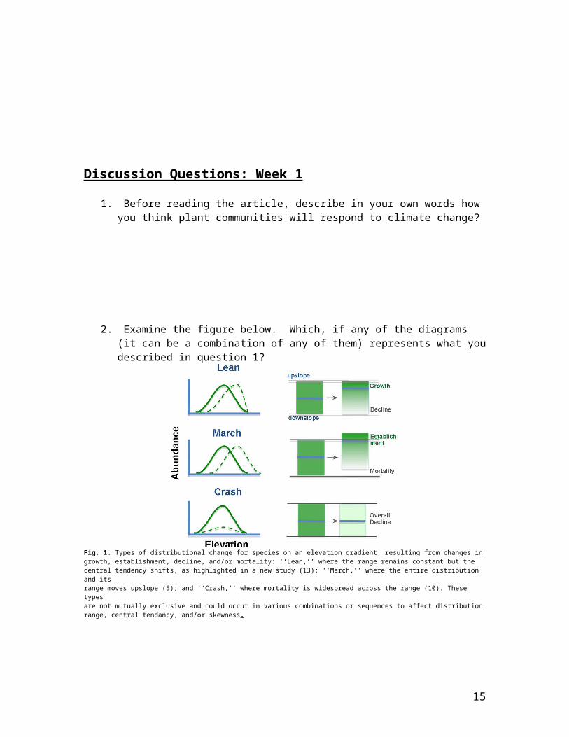
Discussion Questions: Week 1

1. Before reading the article, describe in your own words how you think plant communities will respond to climate change?

2. Examine the figure below. Which, if any of the diagrams (it can be a combination of any of them) represents what you described in question 1?

Fig. 1. Types of distributional change for species on an elevation gradient, resulting from changes ingrowth, establishment, decline, and/or mortality: ‘‘Lean,’’ where the range remains constant but thecentral tendency shifts, as highlighted in a new study (13); ‘‘March,’’ where the entire distribution and itsrange moves upslope (5); and ‘‘Crash,’’ where mortality is widespread across the range (10). These typesare not mutually exclusive and could occur in various combinations or sequences to affect distributionrange, central tendancy, and/or skewness.

3. Which of the diagrams represents what Kelly and Goulden (2008) found in their research in Southern California over a 30 year period?

4. How might the findings from Kelly and Goulden (2008) be applicable to plant communities in southwestern Colorado?

12

5. The authors state four reasons their findings can be attributed to climate change. What are these four reasons and do you agree with them? Why or why not?

6. What would you suggest for future research to expand upon the findings of this study?

13

Relevé Approach to Vegetation Sampling

The relevé approach to vegetation sampling was developed by Braun-Blanquet for application to table analysis for vegetation classification. The primary goal of the relevé approach is to acquire a complete species list from each sample site. If other quantitative site and soil information is collected, the information can also be used for ordination analysis.

Reconnaissance and EntitationReconnaissance is essential. The better your initial knowledge of an area, the better the subsequent sampling will be. This reconnaissance phase should include the establishment of the apparent relations of various vegetation types with topography, history, geology, soil conditions and major disturbance factors (animals, fire, floods, etc.)

The entitation process subjectively subdivides the vegetation into recognizable entities or vegetation types. The types defined during this process are a starting point for analysis of the vegetation. During analysis of the data some of these units will likely be subdivided or eliminated (e.g. they represent transition communities).

Sample Site Requirements for a RelevéThe Braun-Blanquet approach is based on centralized replicate sampling. Plot locations are chosen in the central areas of homogeneous stands of vegetation and numerous replicate samples are collected from other similar sites.

Each sample should satisfy the following criteria:1. Homogeneity of the vegetation canopy2. Homogeneity of the soil and other site factors3. Large enough area to contain all the species in the community4. Should be recognizable as a unit that can be repeated in other areas of the landscape

If the data are to be analyzed using probability statistics, the selection of the sample sites must be done randomly within an area of homogenous vegetation (e.g. stratified random sampling approach)

If the data are to be analyzed using ordination methods, then it is necessary to collect environmental and soils information at each sample site and plant cover estimates.

Plot SizeThere are two main methods for determining plot size: the minimal area technique or using tables based upon previous investigators’ experience.

Minimal areaThe minimum mapping area is determined by finding the point where the species-area curve levels off. Nested plots are used to create this curve. In each plot, a complete species list is created. Additional plots are added until only one or no new species in the larger nested plots are found. The species-area curve does not level off in tropical and other complex communities.

14

Published TablesThe following table is the minimum-area guideline (m2) that has been published by Westhoff and van der Maarel (1978) for various community types. Only a portion of the table is shown.

Pastures 5-10Alpine Meadows 10-50Chaparral 10-100Scrub Communities 25-100Temperate Deciduous Forest 100-500Mixed Forest 200-800Tropical Secondary Rainforest 20-1000

Data to Collect

Site FactorsYou should describe the site as completely as possible using a consistent set of quantitative variables that can be used in an ordination analysis.

SoilsThe soil-vegetation relationship is fundamental to understanding vegetation patterns. Some recommended soil analyses include pH, percent soil moisture, soil texture, percent organic matter, soil nutrients (N, P, K) and other physical and chemical characteristics.

Plant Species You should collect a specimen of every unknown plant species for later verification. Collect the complete plant including roots, stems, leaves, flowers and fruits. Cover estimates should be made for each species. Cover estimates can either be exact aerial estimates or cover-abundance classes can be used. The disadvantage of using cover-abundance classes is that it is not possible to determine the average cover of a species for a group of plots (the average score however can be averaged).

Braun-Blanquet Cover Estimate ScaleR =rare, <<1% cover+ =common, but < 1% cover1 =1-5% cover2 =6-25% cover3 =25.1-50% cover4 =50.1-75% cover5 =75.1-100% cover

15

Size of Plots-Minimal Area Method

16

Cover Class Tables

17

Common Plants of Animas Mountain Trail(partial list)

TreesAbies concolor (White fir)Juniperus osteosperma (Utah Juniper)Juniperus scopulorum (Rocky Mountain Juniper)Pinus edulis (Pinyon Pine)Pinus ponderosa (Ponderosa Pine)Pseudotsuga menziesii (Douglas-fir)Ulmus pumila (Chinese Elm)

ShrubsAmelanchier alnifolia (Utah Serviceberry)Ceanothus fendleri (Buckbrush)Cercocarpus montanus (Mountain Mahogany)Fendlera rupicola (Cliff Fendlerbush)Fragaria virginiana (Wild Strawberry)Gutierrezia sarothrae (Broom Snakeweed)Juniperus communis (Common Juniper)Mahonia repens (Oregon Grape)Peraphyllum ramosissimum (Squawapple)Quercus gambelii (Gambel Oak)Rhus trilobata (Threeleaf Sumac)Rosa woodsii (Wild Rose)Symphoricarpos rotundifolius (Snowberry)

GrassesAchnatherum hymenoides (Indian Ricegrass)Agropyron cristatum (Crested Wheatgrass)Aristida purpurea (Three Awn)Bouteloua gracilis (Blue Grama)Bromopsis inermis (Smooth Brome)Bromus tectorum (Cheat Grass)Elymus elymoides (Squirrel-tail)Festuca arizonica Festuca thurburi Hesperost ipa comata (Needle-and-thread)Koeleria macrantha (June Grass)Muhlenbergia wrightii (Spike Muhley) Pascopyrum smithii (Western Wheatgrass)Poa fendleriana (Muttongrass)Poa pratensis (Kentucky Bluegrass)Sporobolus cryptandrus (Dropseed)

18

Forbs/OthersAchillea lanulosa (Yarrow) Agoseris glauca (Pale Agoseris)Allium acuminatum (Tapertip Onion)Allium cernuum (Nodding Onion)Alyssum alyssoides (Pale Allysum)Androsace septentrionalis (Rock Jasmine)Antennaria parvifolia (Pussytoes)Arabis drummondii (Drummond’s Rockcress)Artemisia franserioides (Sage)Artemisia frigida (Silver Sage)Asclepias subverticillata (Whorled Milkweed)Astragalus coltonii (Milkvetch)Bahia dissecta (Ragleaf Bahia) Calochortus nuttallii (Sego-lily)Castilleja linariifolia (Paintbrush)Chenopodium fremontii (Fremont Goosefoot)Circium tracyi (Thistle)Comandra umbellata (Bastard-Toadflax)Convolvulus arvense (Field Bindweed)Conyza canadensis (Horseweed)Corallorhiza maculate (Summer Coralroot)Delphinium nuttallianum (Larkspur)Erigeron divergens (Fleabane)Erigeron flagellaris (Fleabane)Erigeron speciosus Eriogonum racemosum (Whorled-buckwheat)Erodium cicutarium (Crane’s Bill)Galium septentrionale (Bedstraw)Gaura coccinea (ButterflyWeed)Gayophytum diffusum ssp. parviflorum (Spreading Groundsmoke)Gilia aggregata (Scarlet Gilia)Grindelia squarrosa (Gumweed)Helianthus rigidusHeliomeris multiflora (Showy Goldeneye)Heterotheca villosa (Goldenaster)Hieracium fendleri (Yellow Hawkweed)Holodiscus dumosus (Rock Spiraea)Lactuca serriola (False Dandelion)Lactuca serriola (Prickly-lettuce)Lepidotheca suaveolens (Pineapple Weed)Lithospermum multiflorum (Showy Puccoon)

19

Lotus wrightii (Deer Vetch)Lupinus ammophilus (Lupine)Lupinus kingii (Lupine)Machaeranthera canescensMedicago lupulina (Black Medic)Melilotus officinalis (Yellow Sweet-clover)Opuntia polyacantha (Prickly Pear)Opuntia whipplei (Rat-tailed Cholla)Oreocarpa bakeri Orthocarpus luteus Packera neomexicana (Groundsel)Penstemon barbatus (Beardlip Penstemon)Penstemon linarioides Penstemon rigens Penstemon strictus (Rocky Mountain Penstemon)Penstemon strictus (Rocky Mountain Penstemon)Polygonum aviculare (Knotweed)Psoralidium tenuiflorumPseudocymopterus montanus (Mountain Parsley)Pterogonum alatumSchoenocrambe linifolia (Skeleton Mustard)Solidago simplex (Goldenrod)Sphaeralcea coccinea (Globe Mallow)Taraxacum officinale (Dandelion)Thalictrum fendleri (Meadowrue)Thalpsi montana (Candytuft)Tragopogon pratensis (Salsify)Thermopsis montanusVerbascum thapsus (Mullein)Vicia americana (American Vetch)Virgulus faclcatusWyethia arizonica (Mule’s Ears)Yucca angustissima (Narrow Leaf Yucca)Yucca baccata (Datil Yucca)

20

Quantifying Patterns WorksheetName:_________________________________

1). One thing that plant community ecologists do is describe patterns across various spatial scales. List and define ways to quantify the plant community in the photo above.

Discussion Questions Week 2

21

1. Explain the figure below. Is there anything in the figure that should be removed or added?

2. What makes the “Integrated Community Concept” unique from Clements’ organismic concept or Gleason’s individualistic concept? Do you agree that the IC concept is a stronger theory for understanding the structure and function of ecological systems? Explain your response.

3. How does neutral theory and niche theory fit into the IC concept? Describe both of these theories.

22

4. Why is the IC concept important to consider when thinking about plant community responses to climate change? How, if at all, do the results from Kelly and Goulden (2008) relate to the IC concept?

5. What is a research study that could be conducted in southwest Colorado to test the IC concept and its applicability to climate change?

PC-ORD Multivariate Analysis of Ecological Data Version 6 User’s Booklet

From: McCune, B. and M. J. Mefford. 2011. PC-ORD. Multivariate Analysis ofEcological Data. Version 6. MjM Software, Gleneden Beach, Oregon, U.S.A.

23

24

25

26

27

28

29

30

31

32

33

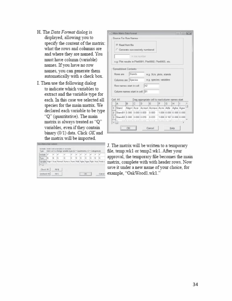
34

35

36

37

38

39

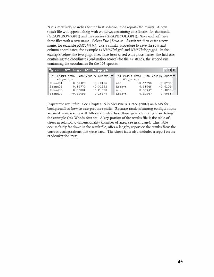
40

41

42

43

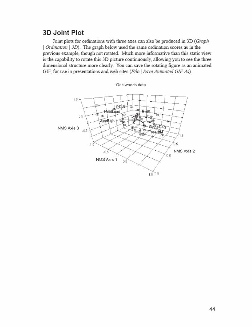
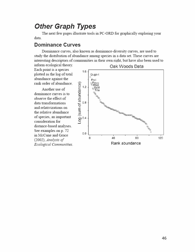
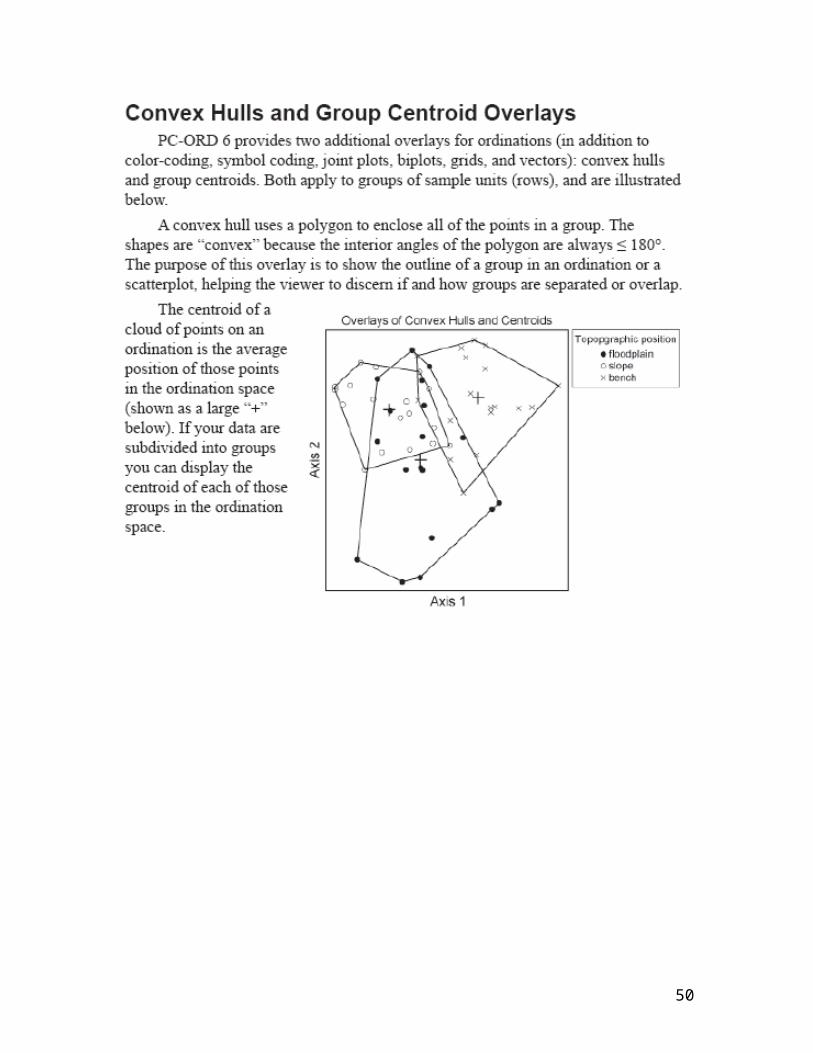
44

Life History Traits Class ExerciseName:_________________________

1. Draw a plant that represents the ideal species. What life history traits does this species have to make it ideal?

2. Why is it not possible to have an ideal plant species?

3. Examine the small and large seeds I have provided for you. One trait of species

survival is to ensure species regeneration. One might hypothesize then that all plants would have numerous, small seeds. Why is this not true?

45

4. Describe the figure below in question #5. What is it trying to explain? NOTE: What does triangle figure does it resemble from a different but related field of science?

5. Highlight the smaller triangles on the figure illustrating what trait or combination of traits best represent different plant functional groups that we have discussed in class. Highlight triangle(s) for Annuals, Biennials, Perennials, & Trees/Shrubs.

46

Intraspecific Competition in Plant Populations Lab—modified from Texas State University “The Ecological Significance of Intraspecific Competition in Plant Populations” exercise #6, no author

DefinitionsInterspecific competition – competition between populations of two or more species in acommunity that relies on similar limiting resources.Intraspecific competition – when populations of one species rely on the same limiting resourceincreasing population density reduces the resources available for individual organisms andthat resource limitation ultimately limits population growth.Density-dependent factor – decreases population growth rate by decreasing reproduction or byincreasing mortality in a crowded population.

Background InformationPlants require resources like nutrients, light, and water to survive, grow, and reproduce. If two organisms that occupy the same habitat rely on a similar resource, and if that resource is present in limited supply (i.e., it’s a limiting resource), then competition will ensue. Competition may involve direct interaction between individuals, such as the release of toxic chemicals (allelopathy). On the other hand, it may occur indirectly when one individual reduces the quantity of resources available to others without coming into direct contact with them. If competing organisms belong to the same species, ecologists refer to their interaction as intraspecific competition. Competitors that belong to different species participate in interspecific competition. Competition is most severe in the case of intraspecific competition because the competitors have almost identical resource needs (their niches are essentially the same). Interspecific competition is more benign because the competing organisms have fewerresource needs in common (their niches share only certain similarities). The greater the resemblance between two coexisting organisms, the more intense the competition.

General Responses of a Population to CompetitionSome familiar models provide predictions about the effects of density-independent and density-dependent factors on the growth rate of a population over time. The former influence theindividuals making up a population regardless of the degree of crowding. The latter varies inimportance as the population size changes. Weather is a density-independent factor. Competitionis a density-dependent factor. How does a population respond to competition? Think about anexperiment in which small populations of a single species are placed in two different situations:

47

When all resources are present in excess, the individuals composing the population are free ofcompetition. In the absence of competition, the population is uninhibited by the consequences ofits own growth (or that of other populations). Therefore, the population grows at its intrinsicrate of increase (r), and it exhibits an J-shaped pattern of exponential expansion in size overtime (the exponential model of population growth).

If at least one resource is limiting, and potentially competing species are absent, then theindividuals belonging to the population will compete only with one another. Such intraspecificcompetition tends to dampen the population’s ability to expand in size. Since intraspecificcompetition increases in intensity as the population becomes larger, it causes a “leveling-off” ofexponential growth. The population is unable to grow indefinitely at its intrinsic rate (r). By thetime the population has reached its equilibrium size (K), intraspecific competition has becomeso severe that further growth is stopped (the change in growth number over time [dN/dt] fallsto zero). The population exhibits an S-shaped pattern of growth over time (the logistic model ofpopulation growth).

The Peculiar Reactions of Plant Populations to CompetitionAnimals and plants respond to competition in fundamentally different ways. Because of thisdifference (among other reasons), ecologists measure the sizes, or densities, of animal and plantpopulations quite differently.

Competition among animals typically causes changes in the numbers of individuals composingpresent and future populations by its influence on birth and death rates. Ecologists generallyexpress the density of an animal population as the number of individuals per unit area.The effects of competition are more complex on plant (and fish) populations: Competition mayalter the birth and death rates of a population (as it does in the majority of animal populations),

48

but it also may bring about developmental changes in individuals. These developmentalmodifications include changes in overall size as well as changes in the number, size, and timingof appearance of each of various organs (e.g., leaves and flowers). Ecologists most commonlyexpress the density of a plant population in terms of biomass per unit area. Biomass is the dryweight of living matter. It can refer to the weight of the above ground tissues of all plantsbelonging to a population, the weight of all leaves, or even the weight of all seeds. As planttissues vary substantially in water content, ecologists usually measure biomass as the weight ofdried plant material.

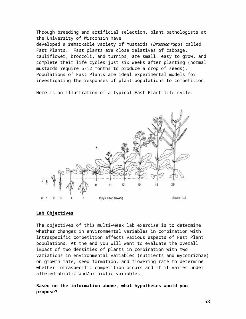
You can take a closer look at the unique responses of a plant population to competition,particularly the developmental changes that typically accompany the struggle for resources by recording the effects of intraspecific competition on populations of “Fast Plants” grown under two different environmental conditions at different densities (i.e., different levels of intraspecific competition).Through breeding and artificial selection, plant pathologists at the University of Wisconsin havedeveloped a remarkable variety of mustards (Brassica rapa) called Fast Plants. Fast plants are close relatives of cabbage, cauliflower, broccoli, and turnips, are small, easy to grow, and complete their life cycles just six weeks after planting (normal mustards require 6-12 months to produce a crop of seeds). Populations of Fast Plants are ideal experimental models for investigating the responses of plant populations to competition.

Here is an illustration of a typical Fast Plant life cycle.

Lab Objectives

The objectives of this multi-week lab exercise is to determine whether changes in environmental variables in combination with intraspecific competition affects various aspects of Fast Plant populations. At the end you will want to evaluate the overall impact of two densities of plants in combination with two variations in environmental variables (nutrients and mycorrizhae) on

49

growth rate, seed formation, and flowering rate to determine whether intraspecific competition occurs and if it varies under altered abiotic and/or biotic variables.

Based on the information above, what hypotheses would you propose?Ho:.. .. ...................... ..Ha:.. .. ...................... ..

Data SetWe will set-up eight treatments:(1) 2 seeds/ 3.5" pot no fertilizer/no mycorrhizae (2) 10 seeds/3.5" pot no fertilizer/no mycorrhizae (3) 2 seeds/ 3.5" pot no fertilizer/mycorrhizae (4) 10 seeds/3.5" pot no fertilizer/mycorrhizae (5) 2 seeds/ 3.5" pot fertilizer/no mycorrhizae (6) 10 seeds/3.5" pot fertilizer/no mycorrhizae (7) 2 seeds/ 3.5" pot fertilizer/mycorrhizae (8) 10 seeds/3.5" pot fertilizer/mycorrhizae

Students will work in groups of 2. We will have six groups. Each group will set up 2 replicates of each treatment (N=12/treatment). Total # of pots= 12 replicates x 8 treatments= 96 total.

Plant Data:1. Onset time of first true leaf/treatment2. Number of plants that survive/treatment3. Mean forage biomass (g)/ plant/treatment4. Mean height of the plants/treatment5. Condition of leaves/treatment

Flower data:1. Onset time of flowers /treatment2. Mean number of flowers/treatment

Reproductive Output data:1. Onset time of seed/treatment2. Mean number of seeds/plant/treatment3. Mean Biomass of seeds/plant/treatment3. Number of seeds/pod (or plant) /treatment (extra credit)

Root Allocation data:1. Mean root biomass (g)/plant/treatment2. Root to forage biomass comparison/treatment

50

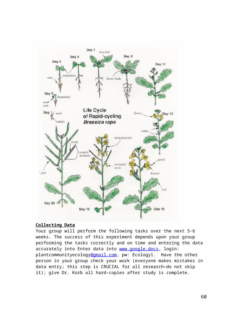
Collecting DataYour group will perform the following tasks over the next 5-6 weeks. The success of this experiment depends upon your group performing the tasks correctly and on time and entering the data accurately into Enter data into www.google.docs, login: [email protected], pw: Ecology1. Have the other person in your group check your work (everyone makes mistakes in data entry; this step is CRUCIAL for all research—do not skip it); give Dr. Korb all hard-copies after study is complete. You will be responsible to track your group pots every 2-3 days to monitor phenological stages of your plants in addition to recording other variables.

Weekly Monitoring SchedulePlanting - Week 11. Each group will plant two replicates of each treatment in 3.5” pots for a total of 16 pots. Fill each pot ½ way. b. Water the soil a little bit.c. Fill the pot the rest of the way with soil and water again.

51

mailto:[email protected]

http://www.google.docs/

d. Now poke small holes where the seeds will go and put the seeds into the pot spaced out.e. Put soil on the seeds and water with a dropper. Do not over water!2. Label your pots by writing the following on masking tape: group name, treatment, replicate #3. Place pots under light table and mark their location on master sheet for pot location.4. Note: today is day 1 of experiment for future phenology recording.

First Leaf Emergence, First Flower Emergence- Week 1-21. Record date and day of experiment for first true leaf emergence and first flower emergence for all eight treatments. 2. Record average leaf condition for each pot/treatment (note this is a categorical value vs quantitative value) once each week entire duration of study.

Flower Counts- Week 31. Count the # of flowers/plant for each pot between day 15-18 to determine mean # of flowers/plant.

Cross-Pollinations –Week 2-31. Using a different cotton-tipped applicator stick for each pot, rotate the applicator stick overthe flowers within the same pot to pick up pollen grains from anthers and distribute them tostigmas. Move pollen back and forth among the different plants within the same pot, butdon’t transfer pollen from one pot to the other.2. Put the applicator stick into the pot and tie the plants together with a wire tie.3. Record the date and day of experiment of cross-pollination.

First Seed Emergence-Week 3-41. Record the date and day of experiment for first seed emergence for all eight treatments.

Harvest Time – Week 51. Remove your group’s pots. Count the number of plants that survived in each pot and record data. and carefully remove each plant from the pots and set a side (do one pot at a time). Save the pots for future labs.2. Measure the height of each plant (from base of leaves to top of plant not including roots)/plot/treatment to determine mean height/treatment. 3. Cut the plant from the roots and place the plant in one bag. Measure root length (longest length) and put the roots in another bag. Mark each bag with group name, treatment, and replicate # and if it is plant or root. Only include live plants. Place the bags, with the top open, in the drying oven.

Weighing – Week 51. Take your group’s brown paper bags out of the drying oven. Carefully remove and weigh theentire contents of each bag.2. Balance Instructions:a) Do NOT move balance—otherwise you will need to re-level balance(b) Do NOT push down on the balance or it will be permanently damaged and unusable!3. Weigh the appropriate variables to the nearest 0.01 g and record your results.4. To separate the seeds, put the pods in an envelope and crush the pods. Transfer the seeds to apetri dish and remove any additional chaff from the pods. Be careful not to allow any of the

52

pod material to become mixed in with the seeds. Count the total number of seeds(“NUMBER OF SEEDS”—this is extra credit) and weigh them in the petri dishes (“BIOMASS OF SEEDS”).Record your results. 5. Enter all of your data into google.docs and have your partner check your data entry. 6. Discard all plant material and the bag in the trash.

Data Analysis/Writing Lab Report—Week 6-91. Follow same format as PC-Ord final report. Include all sections except abstract. 2. You need to include a minimum of 3 plant data, 1 flower, 2 reproductive, and 1 root data for a total of 7 analyses for your final report. Don’t randomly choose these data but think about the story you can tell from your data. You will always have more data than the data you present. The key to being a good researcher is finding what data is interesting to present and tells a story about the study you conducted. Sometimes the data that is interesting is data that showed no significant results; therefore you need to think carefully about what you choose to present. The point of this is not to “hide” data that doesn’t fit your story but to highlight major trends that you saw in your data that can support or refute the current body of literature regarding competition theory. Plant Data:1. Onset time of first true leaf/treatment2. Number of plants that survive/treatment3. Mean forage biomass (g)/ plant/treatment4. Mean height of the plants/treatment5. Condition of leaves/treatment

Flower data:1. Onset time of flowers /treatment2. Mean number of flowers/treatment

Reproductive Output data:1. Onset time of seed/treatment2. Mean number of seeds/plant/treatment3. Mean Biomass of seeds/plant/treatment3. Number of seeds/pod (or plant) /treatment (extra credit)

Root Allocation data:1. Mean root biomass (g)/plant/treatment2. Root to forage biomass comparison/treatment3. Mean root length/treatment

Things to think about and include in report

1. What hypotheses were you testing in your experiments? What reasoning led you to develop these hypotheses?

2. Did your results support your hypothesis? What conclusions can you draw?

53

3. What abiotic or biotic factors in nature might change the competitive outcome you observed? How could you design a similar test in the field?

4. What plant community ecology theories are supported/refuted or simply are relevant to your experiments?

5. How would you improve this study to expand its scope or to better address your initial hypotheses?

54

Plant Interaction WorksheetName:________________________________

1. Draw two plant competing. What are they competing for? Provide a definition for competition. Is your drawing showing intra or inter-competition? Explain these definitions as well.

2. Explain the figure below. What patterns are we seeing and why?

55

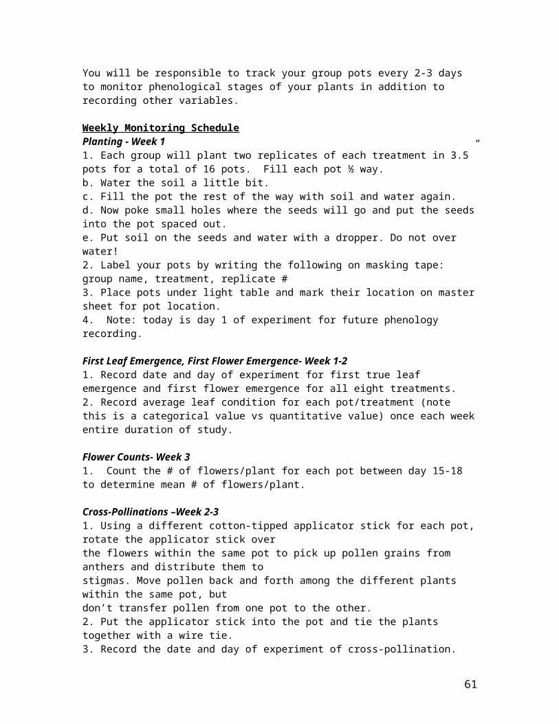
3. Explain the figure below. Which of the two species is the stronger competitor? Would this always be the case? Explain your answer. Define trade-offs and how this related your answer regarding competition.

4. What type of environment would you expect to find competition? A high productive environment with limited disturbance and abiotic stresses or an unproductive environment with abiotic stresses? Explain your answer. Where you would expect to see facilitation—use same environments as above. Again, explain your answer.

56

5. Explain the figure below. A and B represent two different plant species. How does this relate to competition?

6. Early research in chaparral in California in the 1960s saw that there were halos of bare ground surrounding the dominant shrubs, Salvia leaucophylla and Artemisia californica; both species have a pungent aromatic scent. Researchers attributed this to allelopathic chemicals. Define allelopathy. Some researchers questioned this theory and conducted additional research and found in fact that it wasn’t due to allelopathy but something else? What else might have caused these bare ground patches near shrubs? How would you test for this?

57

Study Guide: Plant Community Ecology First Exam

You are responsible for all of our reading discussion questions, in-class worksheets, and lecture material. All of the in-class worksheets and reading discussion questions are fair game for the exam. Please review these sheets. In addition, you are responsible for the material below. Some of the exam questions will draw upon you critically thinking about how our lecture material ties into our reading material so make sure you review everything and know how it fits together.

Week 1/2: Intro to Plant Community Ecology/Gradient Analysis1) What is ecology?2) Know the four ways to study ecology and examples of each (e.g., observation, field experiments…)3) Understand why scale is important both on a temporal and spatial scale when studying ecology.4) What is a microhabitat and why is it important in explaining plant species diversity?5) Know the history of plant ecology and major players (Darwin, Warming)6) Explain the tripod concept in relation to plant community ecology (pattern, process theory)7) Know the different ways to describe the structure of plant communities and be able to define what each means (e.g., richness, density, frequency, evenness, diversity, physiognomy, etc..—there are more)8) Define community? How can it be defined in two different ways spatially?9) Understand in detail the difference between Clements, superorganism concept and Gleason’s individualistic concept. How did their personal backgrounds influence their ideas on plant community assemblage? Be able to tie these concepts to the articles we read and describe the debate in the 1920’s, 1960-2000, and then presently—info from lectures and articles.10) Understand and be able to explain the Integrated Community Concept and how it relates to the debate with Clements and Gleason. For example, what do the filters in the diagram represent?11) What is a species area curve and Gaussian curve related to plants? How have these curves influence how plant ecologists view plant communities?12) What is an ecological niche in reference to plants? What is the difference between a fundamental and realized niche? How does the concept of a niche help explain plant community diversity and how does niche breadth contribute to this?13) What is the competitive exclusion hypothesis? Why does this hypothesis not work in the natural world? Know the details of each topic, not just words (e.g., spatial heterogeneity, temporal variation, competitive ability/dispersal trade-off, etc.) 14) What is the intermediate disturbance hypothesis and why does it postulate that diversity should highest in intermediate vs low or high disturbance?

58

Community Data Analysis Week 2/31. What is the direct and indirect ordination?2. What is the difference between univariate and multivariate data analysis? Provide an example for each. 3. What is the difference between parametric and non-parametric statistical analyses? Provide an example of when you would use each statistical analysis?4. What is the difference between alpha, gamma, and beta diversity?5. What are the five problems with community data? Be able to explain each? For example, what is meant by the zero truncation problem; what information is and is not provided?6. How is community data skewed and how does this impact analyzing community data?

Life History Traits Week 31. What is an ecological optimum and physiological optimum in reference to plant life history traits?2. Define life history and the three types of life cycles (annual, biennial, perennial).3. Understand how trade-offs in life history traits affects individual species and their ability to interact with other species.4. Define fitness and understand how this relates to trade-offs in plants.5. Explain Grime’s CSR Triangle and how MacArthur’s r vs K animal theory influenced Grime’s development of this triangle?6. Give an example and be able to describe life history traits of a stress-tolerator, competitor, and ruderal.7. What are some life history traits related to seed germination that buffer plants against environmental stochasticity? 8. What is masting and why does it occur in plants?9. What abiotic and biotic variables can influence plant phenology? Why is plant phenology important to study?

Species’ Interactions Week 41. Define competition and the differences between intra and interspecific competition.2. What are some abiotic and biotic variables that impact competition? How do plant trade-offs and stochastic environments impact completion as well?3. Understand the history of the debate between Grime and Tilman (1980s) regarding the effects of competition on species coexistence and community composition and where this debate stands today (include Craine’s critique). 4. What are some key differences between Grime and Tilman theories related to light and nutrient competition and what views do they have in common?5. Describe the resource-ratio hypothesis and how it relates to niche theory.

59

6. What are some ways in which plants alter their soil (rhizosphere) environment? What is allelopathy and what are some of the controversies surrounding this research and how might this be alleviated through future research?7. Define facilitation and provide some examples. Are facilitative interactions between specific species always the same or do they vary given the biotic and abiotic environment?8. Define mycorrhizae and some of the numerous benefits to plants. What are some of the differences between arbuscular (endo) and ectomycorrhizae?

60

Fire Science—What is Fire? WorksheetName: ____________________________

1. What 3 elements are needed for fire?

2. Light match. Explain what you are doing and how you think fire occurs from this process?

3. Is fire one ignition, or a series of ignitions? Explain answer.

4. Light candle. Is this an endothermic or exothermic reaction, or both? Provide definitions for both terms and example for each.

Endothermic:

Exothermic:

5. Hold glass jar over candle (do not place the jar over the candle completely). What occurs and why is this occurring?

61

6. Place jar completely over candle. What occurs and why is this occurring?

7. What would happen if you supplied oxygen under the glass so the flame could burn?

8. How do you put out fire?

9. What is FIRE?

10. What are the four phases of fire?

62

Pinyon-Juniper Class Exercise

Pinyon juniper forests vary in their distribution across elevations (5500-8500 ft).Answer the following questions regarding their distribution patterns.

1) In the above diagram draw in the elevation bands for the pinyon-juniper forest life zone. Is there a difference between north and south facing slopes? Why or why not? Why do pinyon-juniper forests only grow between 5500 and 8500 ft? Hint: what are the limiting climatic factors?

2) Pinyon pine and Utah juniper are NOT evenly distributed across the elevation gradient range for pinyon-juniper forests. Which of the two species would be found higher in elevation? ___________________ Lower in elevation?___________________

What physical characteristics for these two species led you to your conclusions—adaptations to different climatic environments?

3) Density and basal area are also NOT evenly distributed across the elevation gradient range for pinyon-juniper forests. Where would density be the highest and why? Where would basal area be the highest and why?

5500 ft

8500 ft.

North facingSouth facing

63

4) Fire is one of the major disturbance agents in pinyon-juniper forests. Is fire behavior similar in intensity and frequency across the elevation gradient? Fill in the fire behavior triangle below and think about how these three variables would influence fire behavior and how they would vary across the elevation gradient. Specifically, look at the leg of the triangle that you graphed in question #1.

64

Fire Behavior Triangle

Mixed Conifer Class Exercise

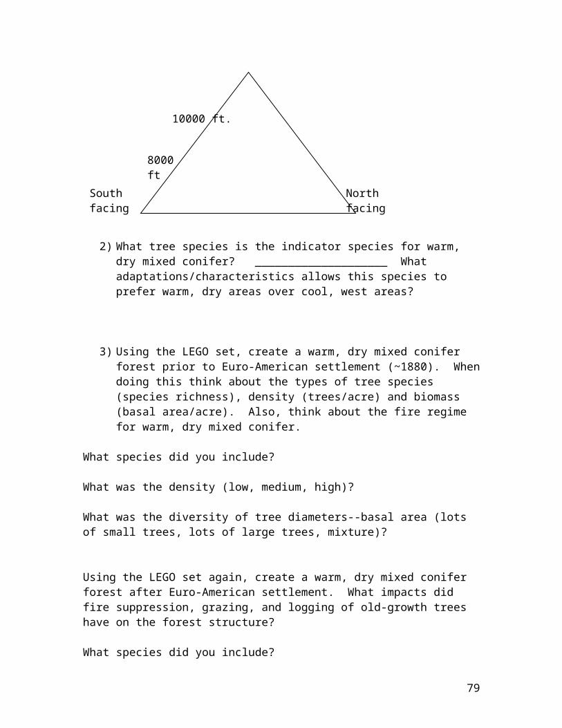
1) There are two types of mixed conifer in the Southwest: warm, dry mixed conifer and cool, wet mixed conifer. How is it possible for these two different vegetation types to grow near each other when their names describing their environment are so different? In the diagram below draw in the elevation bands for these two types of mixed conifer.

2) What tree species is the indicator species for warm, dry mixed conifer? ____________________ What adaptations/characteristics allows this species to prefer warm, dry areas over cool, west areas?

3) Using the LEGO set, create a warm, dry mixed conifer forest prior to Euro-American settlement (~1880). When doing this think about the types of tree species (species richness), density (trees/acre) and biomass (basal area/acre). Also, think about the fire regime for warm, dry mixed conifer.

What species did you include?

What was the density (low, medium, high)?

What was the diversity of tree diameters--basal area (lots of small trees, lots of large trees, mixture)?

Using the LEGO set again, create a warm, dry mixed conifer forest after Euro-American settlement. What impacts did fire suppression, grazing, and logging of old-growth trees have on the forest structure?



8000 ft

10000 ft.


65


4) Using the LEGO set, create a cool, wet mixed conifer forest prior to Euro-American settlement (~1880). When doing this, think about the types of tree species (species richness), density (trees/acre) and biomass (basal area/acre). Also, think about the fire regime for cool, wet mixed conifer.




Using the LEGO set again, create a cool, wet mixed conifer forest now after Euro-American settlement. What impacts did fire suppression, grazing, and logging of old-growth trees have on the forest structure?




5) Fire is one of the major disturbances in mixed conifer forests. Is fire behavior similar in intensity and frequency across the elevation gradient for the two different types of mixed conifer (warm, dry and cool, wet)?

66

Subalpine Class Exercise

1) In the diagram below draw in the elevation band for the subalpine. Note, how does this influence tree line? Where would you first see signs of climate change impacting tree line?

2) The subalpine is dominated by two tree species: subalpine fir and Engelmann spruce. Look at the photographs and think about traits for the other common conifers we have already discussed in class and list four adaptations for each species (some of them can be the same for both species).

10000 ft

11500 ft.


67

Subalpine Fir1)

2)

3)

4)

3) What other tree species that we have already talked about might also occur in the subalpine vegetation zone? What adaptations do these species have to live at higher elevations (colder and wetter than lower elevations)?

68

Engelmann Spruce1)

2)

3)

4)

4) What type of forest stand structure did the subalpine have prior to Euro-American settlement? When describing this think about the types of tree species (species richness), density (trees/acre—low, medium, high) and biomass (basal area/acre-- lots of small trees, lots of large trees, mixture)?

5) What type of forest stand structure did the subalpine have after Euro-American settlement? When describing this think about the types of tree species (species richness), density (trees/acre—low, medium, high) and biomass (basal area/acre-- lots of small trees, lots of large trees, mixture)?

6) Fire is one of the major disturbance agents in the subalpine vegetation zone. Fill in the fire behavior triangle below and think about how these three variables would influence the fire regime for subalpine forests. List the fire regime for subalpine forests and the variables that influence it.

69

Fire Behavior Triangle

PC-Ord Report-Plant Community EcologyPlease include the following components and analyses into your plant community ecology report using PC-Ord and SPSS analyses. I have highlighted the sections I am requiring for this lab report and what you should include because it will be part of the grading matrix.

Writing Lab Reports and Scientific Papersby Warren D. Dolphin, Iowa State University; modified by Julie E. Korb 6/26/2012 Information from: http://www.mhhe.com/biosci/genbio/maderinquiry/writing.html

Format

A scientific report usually consists of the following: 1. Title 2. Abstract 3. Introduction 4. Methods 5. Results 6. Discussion/Conclusion 7. Literature cited 8. Acknowledgments

There is general agreement among scientists that each section of the report should contain specific types of information.

Title

The title should be less than ten words and should reflect the factual content of the paper. Scientific titles are not designed to catch the reader's fancy. A good title is straightforward and uses keywords that researchers in a particular field will recognize.

Abstract

The purpose of an abstract is to allow the reader to judge whether it would serve his or her purposes to read the entire report. A good abstract is a concise (100 to 200 words) summary of the purpose of the report, the data presented, and the author's major conclusions.

Introduction

The introduction defines the subject of the report. It must outline the scientific purpose(s) or objective(s) for the research performed and give the reader sufficient background to understand the rest of the report. Care should be taken to limit the background to whatever is pertinent to the experiment. A good introduction will answer several questions, including the following: Why was this study performed?

70

Answers to this question may be derived from observations of nature or from the literature. What knowledge already exists about this subject? The answer to this question must review the literature, showing the historical development of an idea and including the confirmations, conflicts, and gaps in existing knowledge. (FOR THIS LAB, SIMPLY TIE IN AN INFORMATION FROM PAPERS WE HAVE DISCUSSED IN CLASS, YOU DON’T NEED OTHER LITERATURE RESOURCES)What is the specific purpose of the study? The specific hypotheses and experimental design pertinent to investigating the topic should be described.

Methods

As the name implies, the methods used in the experiments should be reported in this section. The difficulty in writing this section is to provide enough detail for the reader to understand the experiment without overwhelming him or her. When procedures from a lab book or another report are followed exactly, simply cite the work, noting that details can be found in that particular source. However, it is still necessary to describe special pieces of equipment and the general theory of the assays used. Generally, this section attempts to answer the following questions: Where and when was the work done? (This question is most important in field studies.) What methodology was used and how was data collected. Be specific so someone could repeat your study. Review manuscripts that we are reading to see the level of detail needed for this section and break this section into subsections (e.g., study area, experimental design, field methods)Statistical Analyses

Results

The results section should summarize the data from the experiments without discussing their implications. The data should be organized into tables, figures, graphs, photographs, and so on. But data included in a table should not be duplicated in a figure or graph. All figures and tables should have descriptive titles and should include a legend explaining any symbols, abbreviations, or special methods used. Figures and tables should be numbered separately and should be referred to in the text by number, for example:

1. Figure 1 shows that the activity decreased after five minutes. 2. The activity decreased after five minutes (fig. 1).

Figures and tables should be self-explanatory; that is, the reader should be able to understand them without referring to the text. All columns and rows in tables and axes in figures should be labeled. See appendix B for graphing instructions. This section of your report should concentrate on general trends and differences and not on trivial details. Many authors organize and write the results section before the rest of the report.

71

1) Written results sections summarizing major findings that are presented in figures/tables. You can break data up by elevation or aspect or any other categorical variable you decide to divide the data set into (you need equal #s of plots-5 for each level of study). For example 5 low and 5 high elevation sites.

2) Analyses to conduct with data: Make sure you look at your CV to see if your species data needs to be changed (we already determined this in class together; we relativized the data, another option would be to transform the data). Make sure that you do your summary of rows/columns on your raw data or your numbers for cover, diversity, etc. will be incorrect. Do all other analyses on the transformed data in PC-Ord.

a) Summary Data of Species from Sum/Row Columns ( Average Species Richness, Average Shannon or Simpson Diversity Index, Average Plant Cover). Data can be presented in a table or figures

b) Summary Data of Secondary Variables from Sum/Row Columns (Average Elevation, Tree Canopy Cover, Aspect, Litter, etc.). Data can be presented in a table or figures.

c) NMS Ordination (Graph that includes Biplot Data—vectors from the Secondary Matrix)

d) Permanova (Table that shows traditional ANOVA F table and p value)e) Indicator Analysis (Table that shows IV—importance value and p value for only

significant species)

ADDITIONAL ANALYSES-not required, will get extra credit f) Average frequency of individual species. You don’t need to do this for all

species but choose a subset. You can get creative and break into functional groups (grasses, forbs, shrubs, trees, legumes) or (annuals, biennials, perennials).

g) Correlation Analyses of main or secondary matrix variables with axesh) Regression analyses of biotic variable to abiotic variable

Discussion/Conclusion

This section should not just be a restatement of the results but should emphasize interpretation of the data, relating them to existing scientific research (papers), theory and knowledge. Speculation is appropriate, if it is so identified. Suggestions for the improvement of techniques or experimental design may also be included here. In writing this section, you should explain the logic that allows you to accept or reject your original hypotheses. You should also be able to suggest future experiments that might clarify areas of doubt in your results.

Literature Cited

This section lists all articles or books cited in your report. It is not the same as a bibliography, which simply lists references regardless of whether they were cited in the paper. The listing should be alphabetized by the last names of the authors. Different

72

journals require different formats for citing literature. The format that includes the most information is given in the following examples:

For articles:Fox, J.W. 1988. Nest-building behavior of the catbird, Dumetella carolinensis. Journal of Ecology 47: 113-17. For Books:Bird, W.Z. 1990. Ecological aspects of fox reproduction. Berlin: Guttenberg Press.

For chapters in books:Smith, C.J. 1989. Basal cell carcinomas. In Histological aspects of cancer, ed. C.D. Wilfred, pp. 278-91. Boston: Medical Press. When citing references in the text, do not use footnotes; instead, refer to articles by the author's name and the date the paper was published. For example:

1. Fox in 1988 investigated the hormones on the nest-building behavior of catbirds. 2. Hormones are known to influence the nest-building behavior of catbirds (Fox,

1988).

When citing papers that have two authors, both names must be listed. When three or more authors are involved, the Latin et al. (et alia) meaning "and others" may be used. A paper by Smith, Lynch, Merrill, and Beam published in 1989 would be cited in the text as: Smith et al. (1989) have shown that... This short form is for text use only. In the Literature Cited, all names would be listed, usually last name preceding initials.There are a number of style manuals that provide detailed directions for writing scientific papers. Some are listed in further readings at the end of this section.

Acknowledgments

Include funding sources for projects, individuals who assisted in project, and any other individuals that contributed to the success of the project.

General Comments on Style

1. All scientific names (genus and species) must be italicized. (Underlining indicates italics in a typed paper.)

2. Use the metric system of measurements. Abbreviations of units are used without a following period.

3. Be aware that the word data is plural while datum is singular. This affects the choice of a correct verb. The word species is used both as a singular and as a plural.

4. Numbers should be written as numerals when they are greater than ten or when they are associated with measurements; for example, 6 mm or 2 g but two

73

explanations of six factors. When one list includes numbers over and under ten, all numbers in the list may be expressed as numerals; for example, 17 sunfish, 13 bass, and 2 trout. Never start a sentence with numerals. Spell all numbers beginning sentences.

5. Be sure to divide paragraphs correctly and to use starting and ending sentences that indicate the purpose of the paragraph. A report or a section of a report should not be one long paragraph.

6. Every sentence must have a subject and a verb. 7. Avoid the use of slang and the overuse of contractions. 8. Use active voice.

Sample Tables/Figures (these are from other studies but should give you an idea of formatting).

74

75

Fig. 4. Non-metric multidimensional scaling ordination of untransformed tree basal area of species reconstructed for 1870 (reference condition), pretreatment 2003 and post-treatment 2009. Each symbol represents one unit for 1 year (N = 12/year). The final solution had three dimensions, stress = 14.52 and P = 0.02.

76

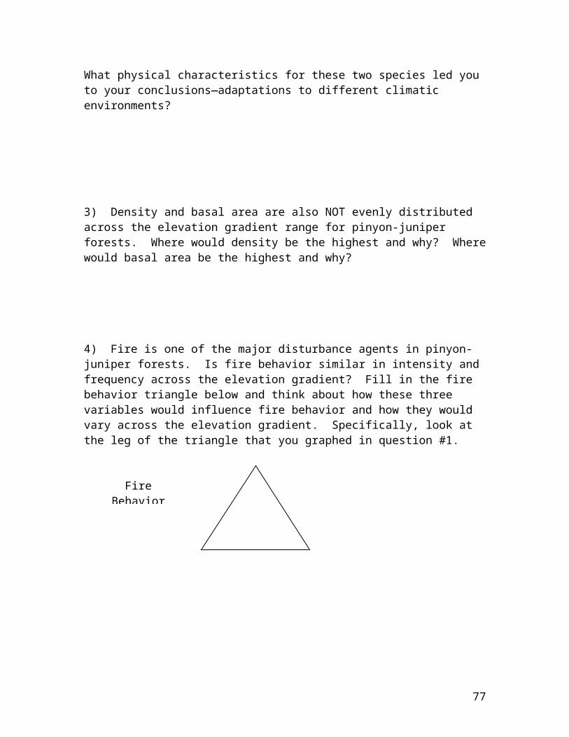
Table 2. Forest structure (trees taller than breast height (137 cm) for Control, Thin/Burn, and Burn treatments. Data values are shown from measurements carried out prior to treatments in 2003, followed by percentage change (positive or negative) as measured after treatment in 2009.Treatment Total ABCO PIEN PIPO POTR PSME

Tree density (trees ha-1)Control (pretreatment) 735.0 364.7 48.8 180.9 140.6Percentage change -22 -20 -3 -39 -9Thin/Burn (pretreatment) 706.9 444.7 0.3 60.9 174.1 26.6Percentage change -82 -96 -100 -32 -65 -76Burn (pretreatment) 590.0 366.6 0.6 57.2 83.1 82.5Percentage change -37 -42 0 -8 - 48 -22Basal Area (m2 ha-1)Control (pretreatment) 29.6 9.3 9.5 3.8 7.0Percentage change -9 -21 5 -23 -8Thin/Burn (pretreatment) 25.6 10.3 0.04 10.6 3.0 1.6Percentage change -49 -86 -100 -8 -64 -45Burn (pretreatment) 25.8 9.1 0.1 9.4 1.8 5.3Percentage change -16 -29 9 -0.2 -22 -21

SAMPLE WRITTEN RESULTS FOR TABLE 2 AND FIGURE 4 ABOVEResultsFOREST STRUCTURE

There were no significant differences in total tree density (U= 2.81, P= 0.25) or basal area (U= 2.44, P= 0.29) among units prior to restoration in 2003. In 2009, following treatments, total density (U= 9.27, P= 0.01) and basal area (U= 9.85, P= 0.007) were significantly lower in thin/burn units than the control and burn units (Table 2). Thin/burn units had the only significant (Z= 2.17, P= 0.03) change in tree density with an 82% decline between pre (709.6 trees ha-1) and post-treatment (126.9 trees ha-1) largely from significant decreases, 96%, in white fir (Z= 2.17, P= 0.03) and, 76%, in Douglas-fir (Z= 2.03, P= 0.03) (Table 2). In 2009, total basal area differences among treatments were driven by significant differences in Douglas-fir basal area (U= 8.8, P= 0.013). Thin/burn units had the only significant decrease in basal area (Z= 2.17, P= 0.03) declining 49% between pre- (25.6 m2 ha-1) and post-treatment (13.1 m2 ha-1) with white fir having the largest decrease of 86% (Z= 2.17, P= 0.03) (Table 2).

Diameter distributions in 2003 for all units prior to restoration followed the reverse-J distribution with a strong dominance of small trees, especially aspen and white fir (Fig. 2). All units had trees at least through the 85-cm diameter class with most of the trees in the 45-cm class and above being ponderosa pine (Fig. 2). After treatment, diameter distributions in the controls were relatively unchanged except for a decrease of small aspen ramets (Fig. 2). Diameter distributions post-treatment in the burn units were unimodal with a peak at the 25-cm diameter class and a relatively gentle decline of the diameter distribution curve to higher values. The main shifts were decreases in white fir in the 5, 15, and 25-cm diameter classes (Fig. 2). Diameter distributions post-treatment

77

in the thin/burn units did not strongly follow any distribution curve (Fig. 2). After treatment, all units maintained trees at least through the 85-cm diameter class with ponderosa pine dominating trees in the 45-cm class and above (Fig. 2).

There was a significant difference in tree basal area between reconstructed 1870, 2003 pre-treatment and 2009 post-treatment data (F = 9.6; P = 0.001) (Table 7). There was also a significant difference between reconstructed 1870, 2003 pre-treatment and 2009 post-treatment data for tree density (F = 14.4; P = 0.0002) (Table 7). There were no differences among blocks across time for tree basal area (F = 1.53; P = 0.07) or tree density (F = 1.12; P = 0.35) (Table 7).Tree basal area by species in 2009 in the thin/burn treatments showed a strong directional shift away from 2003 pretreatment data towards the reconstructed 1870 forest structure (Fig. 4). Burn treatments in 2009 were separated from controls in the same year but did not resemble reconstructed 1870 forest structure (Fig. 4). Indicator species analysis detected species that were particularly consistent indicators for time (Table 8). White fir, Douglas-fir, and aspen were all indicator species for the pretreatment 2003; there were no indicator species for 2009 post-treatment (Table 8).

Study Guide: Plant Community Ecology Second Exam

78

You are responsible for all of our reading discussion questions, in-class worksheets, and lecture material. All of the in-class worksheets and reading discussion questions are fair game for the exam. Please review these sheets. In addition, you are responsible for the material below. Some of the exam questions will draw upon you critically thinking about how our lecture material ties into our reading material so make sure you review everything and know how it fits together.

Species Interactions1. What is allelopathy and what are some ways to improve future alleopathic research? 2. Define facilitation and provide examples of facilitation among plants?3. What are the two main types of mycorrhizae, explain how they are different and what

some of the benefits are for plants to form associations with mycorrhizae?

Pinyon-Juniper1. What are the main adaptations of pinyon pine and Utah juniper to their environment?2. What are the 3 major types of pinyon-juniper habitat as described by Romme and how are they different (soil type, topography, tree density, fire regime)?3. Describe Ips beetle life cycle and how beetles affect stand dynamics in P-J?

Fire as a natural disturbance process1. Review all questions and definitions from fire science in-class exercises2. Know the difference between flaming and smoldering combustion.3. Know why fire and decay is the reverse process of photosynthesis.4. Know the 3 basic types of fire behavior (ground, surface, crown).

Ponderosa Pine/Mixed Conifer1. What are the two major types of mixed conifer forests and what are their distinguishing characteristics (stand composition, stand density, stand basal area, fire regime)?2. Know how to distinguish between the major tree species (e.g., ponderosa pine, Douglas-fir, white fir, aspen, blue spruce).3. What is the natural fire regime for ponderosa pine forests and how and why has this community changed since Euro-American settlement? What are the 3 major causes of changes to forests from Euro-American settlement? 4. What is SAD, what are major causal agents, know about general aspen biology (e.g., how does it regenerate, different types—stable, successional, why does it foster high biological diversity)

Subalpine Forests1. What are the major characteristics of subalpine forests?2. Know how to distinguish between the major tree species (e.g., aspen, lodgepole pine, subalpine fir, Engelmann spruce)3. Know adaptations of the tree species3. Know about major disturbances (fire, avalanche, insect infestations) in subalpine forests and how this affects tree regeneration.

Dendrochronology

79

1. What are the seven major principles of dendrochronology?2. What is a limiting factor in terms of dendrochronology and what is the limiting factor

for tree growth in the Southwest?3. What is crossdating and how do you use a skeleton plot to date wood with no known

age?4. What is a master chronology and how is it used in crossdating?

General Information for all Vegetation Zones1. Have a basic understanding of how each plant community is unique (e.g., aspen can

fall under two different stand types: stable and successional)2. Understand major disturbance agents within each vegetation zone and how they

impact landscape dynamics (e.g., how do insects (Ips beetles affect stand dynamics in pinyon-juniper; how does grazing impact fire in ponderosa pine)?

3. Be able to distinguish the major tree species and know diagnostic (key) characteristics for species—e.g., which vegetation is more susceptible to wind and why? What are two diagnostic characteristics to distinguish spruce from fir?

4. Describe the fire regime, fire intensity, fire frequency, and major species in the different forest types found along an elevational gradient in Colorado.

5. Describe adaptations of specific tree species mentioned in to different fire regimes (e.g., how is the fire regime between lodgepole pine and ponderosa pine different and what are adaptations for both of these species that are specific to their unique fire regimes, draw the aspen triangle and the factors that influence aspen growth)? (review worksheets).

80

Date post:	03-Jul-2018
Category:	Documents
Upload:	phungque
View:	215 times
Download:	0 times

Ecology of the Southwest-Lab #1faculty.fortlewis.edu/korb_j/Plant Community Ecology 2010... · Web...

Documents