52
Qualitative and Limited Dependent Variable Models Adapted from Vera Tabakova’s notes ECON 4551 Econometrics II Memorial University of Newfoundland

Qualitative and Limited Dependent Variable
Models
Adapted from Vera Tabakova’s notes
ECON 4551
Econometrics II
Memorial University of Newfoundland

16.1 Models with Binary Dependent Variables
16.2 The Logit Model for Binary Choice
16.3 Multinomial Logit
16.4 Conditional Logit
16.5 Ordered Choice Models
16.6 Models for Count Data
16.7 Limited Dependent Variables
Slide 16-2Principles of Econometrics, 3rd Edition

Examples:
An economic model explaining why some individuals take a
second, or third, job and engage in “moonlighting.”
An economic model of why the federal government awards
development grants to some large cities and not others.
An economic model explaining why someone is in the labour force
or not
Slide16-3Principles of Econometrics, 3rd Edition
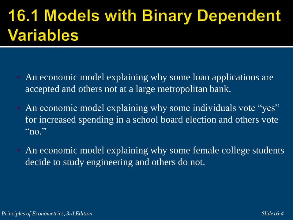
An economic model explaining why some loan applications are
accepted and others not at a large metropolitan bank.
An economic model explaining why some individuals vote “yes”
for increased spending in a school board election and others vote
“no.”
An economic model explaining why some female college students
decide to study engineering and others do not.
Slide16-4Principles of Econometrics, 3rd Edition
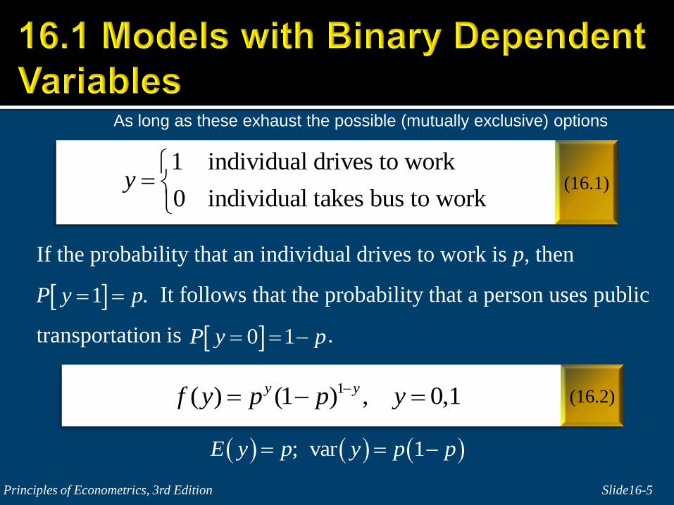
If the probability that an individual drives to work is p, then
It follows that the probability that a person uses public
transportation is .
Slide16-5Principles of Econometrics, 3rd Edition
(16.1)
(16.2)
1 individual drives to work
0 individual takes bus to worky
1 .P y p
0 1P y p
1( ) (1 ) , 0,1y yf y p p y
; var 1E y p y p p
As long as these exhaust the possible (mutually exclusive) options

Slide16-6Principles of Econometrics, 3rd Edition
(16.3)
(16.5)
(16.4)
( )y E y e p e
1 2( )E y p x
1 2( )y E y e x e

One problem with the linear probability model is that the error term is
heteroskedastic; the variance of the error term e varies from one
observation to another.
Slide16-7Principles of Econometrics, 3rd Edition
y value e value Probability
1
0
1 21 x
1 2x
1 2p x
1 21 1p x

Using generalized least squares, the estimated variance is:
Slide16-8Principles of Econometrics, 3rd Edition
(16.6)
1 2 1 2var 1e x x
2
1 2 1 2ˆ var 1i i i ie b b x b b x
*
*
* 1 * *
1 2
ˆ
ˆ
ˆ
i i i
i i i
i i i i
y y
x x
y x e
So the problem of heteroskedasticity
is not insurmountable…

Slide16-9Principles of Econometrics, 3rd Edition
(16.7)
(16.8)
1 2p̂ b b x
2
dp
dx

Problems:
We can easily obtain values of that are less than 0 or greater than 1
Some of the estimated variances in (16.6) may be negative, so the
WLS would not work
Of course, the errors are not distributed normally
R2 is usually very poor and a questionable guide for goodness of fit
Slide16-10Principles of Econometrics, 3rd Edition
p̂
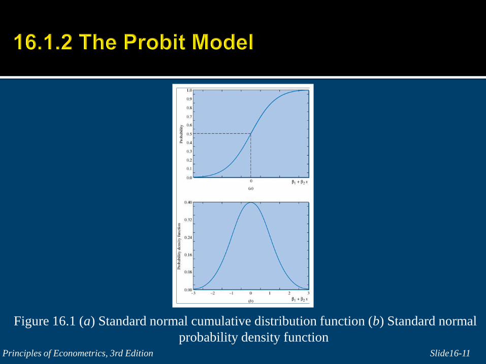
Figure 16.1 (a) Standard normal cumulative distribution function (b) Standard normal
probability density functionSlide16-11Principles of Econometrics, 3rd Edition
Slide16-12Principles of Econometrics, 3rd Edition
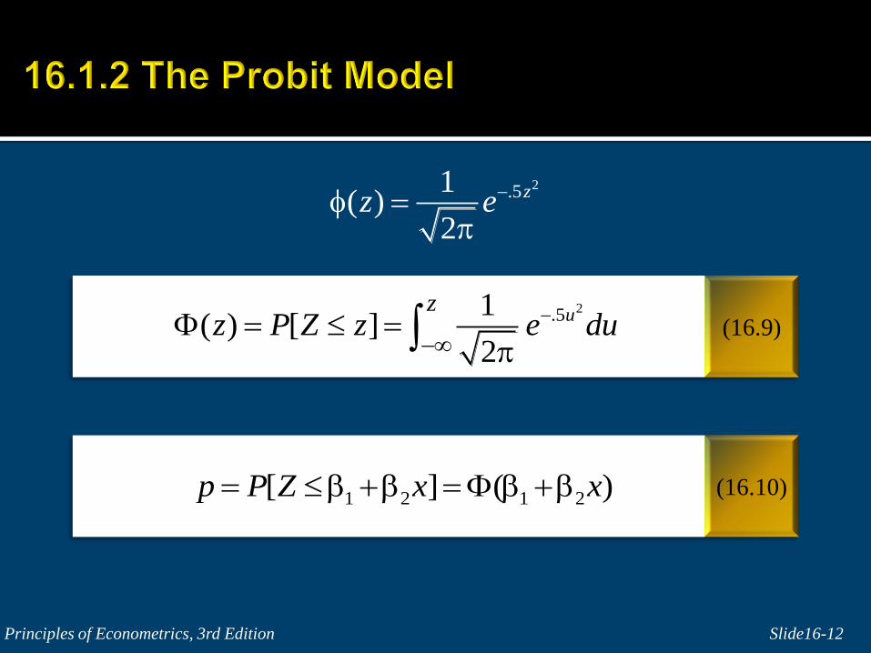
(16.9)
p̂
2.51( )
2
zz e
2.51( ) [ ]
2
uz
z P Z z e du
(16.10)1 2 1 2[ ] ( )p P Z x x
where and is the standard normal probability
density function evaluated at
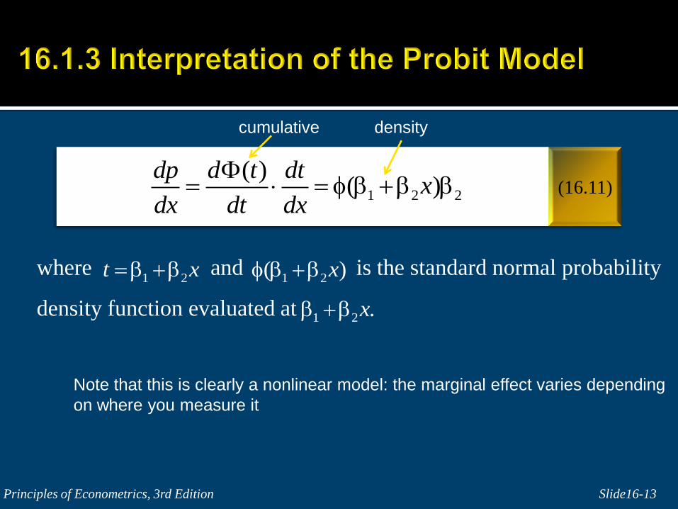
Slide16-13Principles of Econometrics, 3rd Edition
(16.11)1 2 2
( )( )
dp d t dtx
dx dt dx
1 2t x 1 2( )x
1 2 .x
Note that this is clearly a nonlinear model: the marginal effect varies depending
on where you measure it
cumulative density

Equation (16.11) has the following implications:
1. Since is a probability density function its value is always
positive. Consequently the sign of dp/dx is determined by the sign of
2. In the transportation problem we expect 2 to be positive so that
dp/dx > 0; as x increases we expect p to increase.
Slide16-14Principles of Econometrics, 3rd Edition
1 2( )x
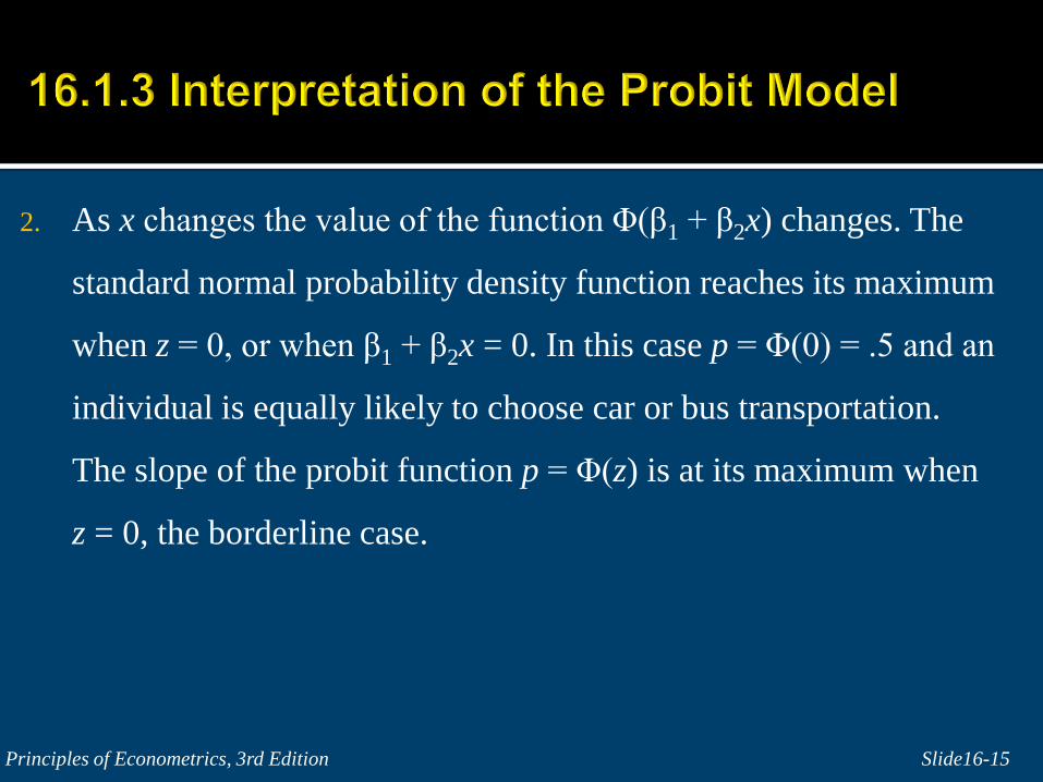
2. As x changes the value of the function Φ(β1 + β2x) changes. The
standard normal probability density function reaches its maximum
when z = 0, or when β1 + β2x = 0. In this case p = Φ(0) = .5 and an
individual is equally likely to choose car or bus transportation.
The slope of the probit function p = Φ(z) is at its maximum when
z = 0, the borderline case.
Slide16-15Principles of Econometrics, 3rd Edition

3. On the other hand, if β1 + β2x is large, say near 3, then the
probability that the individual chooses to drive is very large and
close to 1. In this case a change in x will have relatively little effect
since Φ(β1 + β2x) will be nearly 0. The same is true if β1 + β2x is a
large negative value, say near 3. These results are consistent with
the notion that if an individual is “set” in their ways, with p near 0 or
1, the effect of a small change in commuting time will be negligible.
Slide16-16Principles of Econometrics, 3rd Edition

Predicting the probability that an individual chooses the alternative
y = 1:
Slide16-17Principles of Econometrics, 3rd Edition
(16.12)1 2ˆ ( )p x
ˆ1 0.5ˆ
ˆ0 0.5
py
p
Although you have to
be careful with this
Interpretation!

Suppose that y1 = 1, y2 = 1 and y3 = 0.
Suppose that the values of x, in minutes, are x1 = 15, x2 = 20 and x3 = 5.
Slide16-18Principles of Econometrics, 3rd Edition
(16.13)1
1 2 1 2( ) [ ( )] [1 ( )] , 0,1i iy y
i i i if y x x y
1 2 3 1 2 3( , , ) ( ) ( ) ( )f y y y f y f y f y
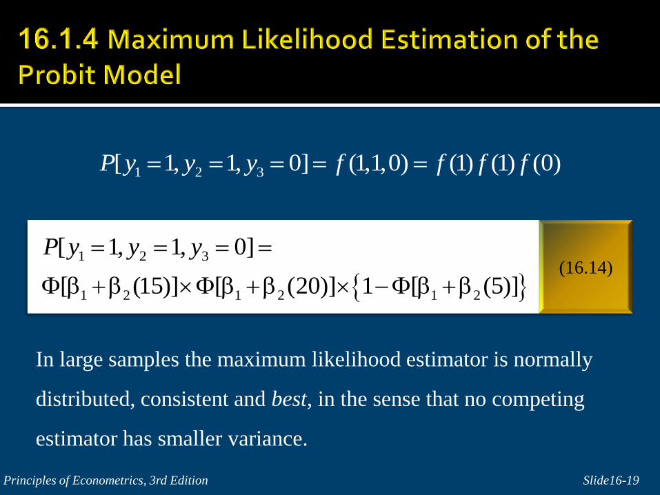
In large samples the maximum likelihood estimator is normally
distributed, consistent and best, in the sense that no competing
estimator has smaller variance.
Slide16-19Principles of Econometrics, 3rd Edition
(16.14)
1 2 3[ 1, 1, 0] (1,1,0) (1) (1) (0)P y y y f f f f
1 2 3
1 2 1 2 1 2
[ 1, 1, 0]
[ (15)] [ (20)] 1 [ (5)]
P y y y

Slide16-20Principles of Econometrics, 3rd Edition

Slide16-21Principles of Econometrics, 3rd Edition
(16.15)1 2 .0644 .0299
(se) (.3992) (.0103)
i iDTIME DTIME
1 2 2( ) ( 0.0644 0.0299 20)(0.0299)
(.5355)(0.0299) 0.3456 0.0299 0.0104
dpDTIME
dDTIME
Marginal effect of DT
Measured at
DTIME = 20
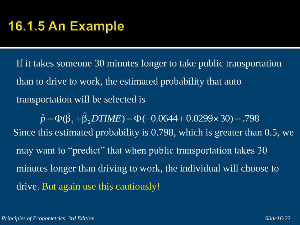
If it takes someone 30 minutes longer to take public transportation
than to drive to work, the estimated probability that auto
transportation will be selected is
Since this estimated probability is 0.798, which is greater than 0.5, we
may want to “predict” that when public transportation takes 30
minutes longer than driving to work, the individual will choose to
drive. But again use this cautiously!
Slide16-22Principles of Econometrics, 3rd Edition
1 2ˆ ( ) ( 0.0644 0.0299 30) .798p DTIME

In STATA:
Use transport.dta
Slide16-23Principles of Econometrics, 3rd Edition
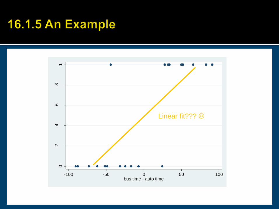
auto 21 .4761905 .5117663 0 1 dtime 21 -1.223809 56.91037 -90.7 91 bustime 21 48.12381 34.63082 1.6 91.5 autotime 21 49.34762 32.43491 .2 99.1 Variable Obs Mean Std. Dev. Min Max
. sum
Slide16-24
0.2
.4.6
.81
= 1
if au
to c
hose
n
-100 -50 0 50 100bus time - auto time
Linear fit???

Slide16-25Principles of Econometrics, 3rd Edition
Understand but
do not use this one!!!
You can
choose
p-values
What is the meaning
of this test?
NORMAL distribution
Not t distribution, because
the properties of the probit
are asymptotic

Principles of Econometrics, 3rd Edition 26
Evaluates at the means by default too
dtime .0119068 .0041 2.90 0.004 .003871 .019942 -1.22381 variable dy/dx Std. Err. z P>|z| [ 95% C.I. ] X = .45971697 y = Pr(auto) (predict)Marginal effects after probit
. mfx compute
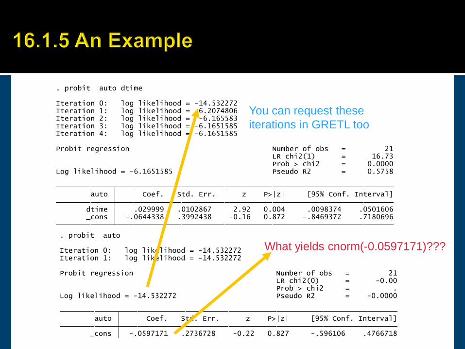
_cons -.0644338 .3992438 -0.16 0.872 -.8469372 .7180696 dtime .029999 .0102867 2.92 0.004 .0098374 .0501606 auto Coef. Std. Err. z P>|z| [95% Conf. Interval]
Log likelihood = -6.1651585 Pseudo R2 = 0.5758 Prob > chi2 = 0.0000 LR chi2(1) = 16.73Probit regression Number of obs = 21
Iteration 4: log likelihood = -6.1651585 Iteration 3: log likelihood = -6.1651585 Iteration 2: log likelihood = -6.165583 Iteration 1: log likelihood = -6.2074806 Iteration 0: log likelihood = -14.532272
. probit auto dtime
Slide16-27
_cons -.0644338 .3992438 -0.16 0.872 -.8469372 .7180696 dtime .029999 .0102867 2.92 0.004 .0098374 .0501606 auto Coef. Std. Err. z P>|z| [95% Conf. Interval]
Log likelihood = -6.1651585 Pseudo R2 = 0.5758 Prob > chi2 = 0.0000 LR chi2(1) = 16.73Probit regression Number of obs = 21
Iteration 4: log likelihood = -6.1651585 Iteration 3: log likelihood = -6.1651585 Iteration 2: log likelihood = -6.165583 Iteration 1: log likelihood = -6.2074806 Iteration 0: log likelihood = -14.532272
. probit auto dtime
_cons -.0597171 .2736728 -0.22 0.827 -.596106 .4766718 auto Coef. Std. Err. z P>|z| [95% Conf. Interval]
Log likelihood = -14.532272 Pseudo R2 = -0.0000 Prob > chi2 = . LR chi2(0) = -0.00Probit regression Number of obs = 21
Iteration 1: log likelihood = -14.532272 Iteration 0: log likelihood = -14.532272
. probit auto
You can request these
iterations in GRETL too
What yields cnorm(-0.0597171)???

Principles of Econometrics, 3rd Edition
This is a probability

Slide16-29
IN STATA
* marginal effects
mfx
mfx,at (dtime=20)
* direct calculation
nlcom (normalden(_b[_cons]+_b[dtime]*30)*_b[dtime] )
and
nlcom (normal(_b[_cons]+_b[dtime]*30) )
Slide16-30Principles of Econometrics, 3rd Edition
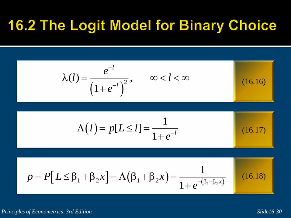
(16.16)
2( ) ,
1
l
l
el l
e
(16.18)
(16.17) 1
[ ]1 l
l p L le
1 21 2 1 2
1
1x
p P L x xe

Slide16-31Principles of Econometrics, 3rd Edition
1 2
1 2
1 2
exp1
1 exp1x
xp
xe
1 2
11
1 expp
x
P i
1P i odds ratio exp1 2X so

Slide16-32Principles of Econometrics, 3rd Edition
P i
1P i odds ratio exp1 2X so
ln P i
1P i 1 2X
So the “logit”, the log-odds, is actually a fully linear function of X

1. As Probability goes from 0 to 1, logit goes from –infinite to +
infinite
2. The logit is linear, but the probability is not
3. The explanatory variables are individual specific, but do not
change across alternatives
4. The slope coefficient tells us by how much the log-odds changes
with a unit change in the variable
Slide16-33
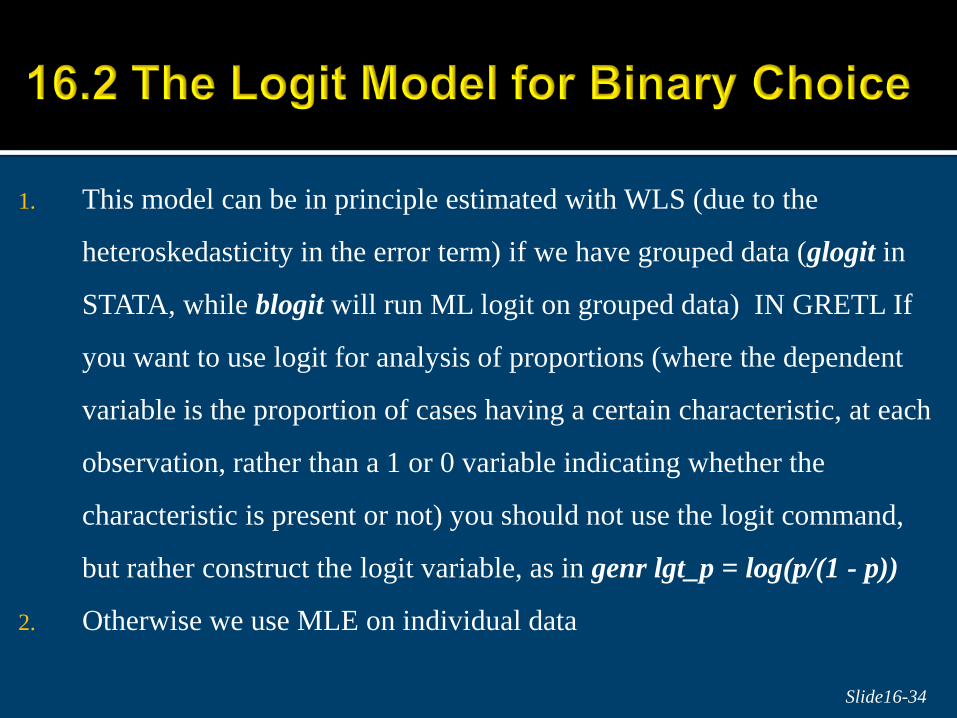
1. This model can be in principle estimated with WLS (due to the
heteroskedasticity in the error term) if we have grouped data (glogit in
STATA, while blogit will run ML logit on grouped data) IN GRETL If
you want to use logit for analysis of proportions (where the dependent
variable is the proportion of cases having a certain characteristic, at each
observation, rather than a 1 or 0 variable indicating whether the
characteristic is present or not) you should not use the logit command,
but rather construct the logit variable, as in genr lgt_p = log(p/(1 - p))
2. Otherwise we use MLE on individual data
Slide16-34

McFadden’s pseudo R2 (remember that it does not have any
natural interpretation for values between 0 and 1)
Count R2 (% of correct predictions) (dodgy but
common!)
Etc.
Measures of goodness of fit are of secondary
importance
What counts is the sign of the regression
coefficients and their statistical and practical
significance
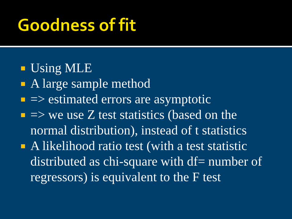
Using MLE
A large sample method
=> estimated errors are asymptotic
=> we use Z test statistics (based on the
normal distribution), instead of t statistics
A likelihood ratio test (with a test statistic
distributed as chi-square with df= number of
regressors) is equivalent to the F test

ho
BIC used by Stata: 18.419 AIC used by Stata: 16.330BIC: -45.516 BIC': -13.690AIC: 0.778 AIC*n: 16.330Count R2: 0.905 Adj Count R2: 0.800Variance of y*: 3.915 Variance of error: 1.000McKelvey & Zavoina's R2: 0.745 Efron's R2: 0.649ML (Cox-Snell) R2: 0.549 Cragg-Uhler(Nagelkerke) R2: 0.733McFadden's R2: 0.576 McFadden's Adj R2: 0.438 Prob > LR: 0.000D(19): 12.330 LR(1): 16.734Log-Lik Intercept Only: -14.532 Log-Lik Full Model: -6.165
Measures of Fit for probit of auto
See http://www.soziologie.uni-halle.de/langer/logitreg/books/long/stbfitstat.pdf
How do you obtain this?

Correctly classified 90.48% False - rate for classified - Pr( D| -) 9.09%False + rate for classified + Pr(~D| +) 10.00%False - rate for true D Pr( -| D) 10.00%False + rate for true ~D Pr( +|~D) 9.09% Negative predictive value Pr(~D| -) 90.91%Positive predictive value Pr( D| +) 90.00%Specificity Pr( -|~D) 90.91%Sensitivity Pr( +| D) 90.00% True D defined as auto != 0Classified + if predicted Pr(D) >= .5
Total 10 11 21 - 1 10 11 + 9 1 10 Classified D ~D Total True
Probit model for auto
. lstat
So in STATA
The “ones” do not
Really have to be
Actual ones, just
Non-zeros
IN GRETL if you do
not have a binary
Dependent variable
It is assumed
Ordered unless
specified multinomial.
If not discrete: error!
But be very careful with these
measures!

To compute the deviance of the residuals:predict “newname”, deviance
The deviance for a logit model is like the RSS in OLS. The smaller the deviance the better the fit.
And (Logit only) to combine with information about leverage:predict “newnamedelta”, ddeviance
(A recommended cut-off value for the ddeviance is 4)

13. .0708038 pred
. list pred if delta>4
. predict delta, ddeviance
. predict dev, deviance
. predict pred, p
_cons -.2375754 .7504766 -0.32 0.752 -1.708483 1.233332 dtime .0531098 .0206423 2.57 0.010 .0126517 .093568 auto Coef. Std. Err. z P>|z| [95% Conf. Interval]
Log likelihood = -6.1660422 Pseudo R2 = 0.5757 Prob > chi2 = 0.0000 LR chi2(1) = 16.73Logistic regression Number of obs = 21
. logit auto dtime, nolog
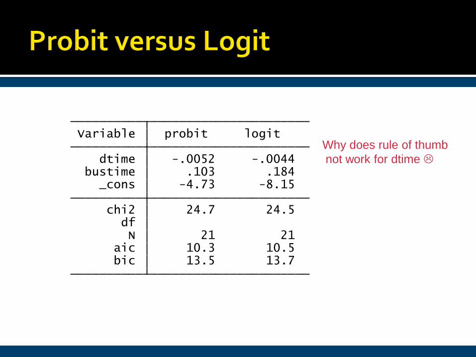
bic 13.5 13.7 aic 10.3 10.5 N 21 21 df chi2 24.7 24.5 _cons -4.73 -8.15 bustime .103 .184 dtime -.0052 -.0044 Variable probit logit
Why does rule of thumb
not work for dtime

A matter of taste nowadays, since we all have
good computers
The underlying distributions share the mean of
zero but have different variances:
Logit
And normal 1
So estimated slope coefficients differ by a
factor of about 1.8 ( ) . Logit ones are
bigger
2
3
3

Watch out for “perfect predictions”
Luckily STATA will flag them for you and drop
the culprit observations
Gretl has a mechanism for preventing the algorithm from iterating endlessly in search of a nonexistent maximum. One sub-case of interest is when the perfect prediction problem arises because of a single binary explanatory variable. In this case, the offending variable is dropped from the model and estimation proceeds with the reduced specification.
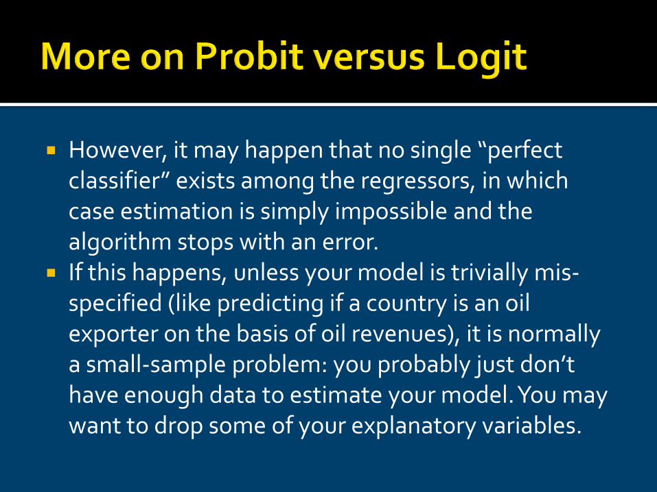
However, it may happen that no single “perfect classifier” exists among the regressors, in which case estimation is simply impossible and the algorithm stops with an error.
If this happens, unless your model is trivially mis-specified (like predicting if a country is an oil exporter on the basis of oil revenues), it is normally a small-sample problem: you probably just don’t have enough data to estimate your model. You may want to drop some of your explanatory variables.

Learn about the test (Wald tests based on chi-
2) and lrtest commands (LR tests), so you can
test hypotheses as we did with t-tests and F
tests in OLS
They are asymptotically equivalent but can
differ in small samples
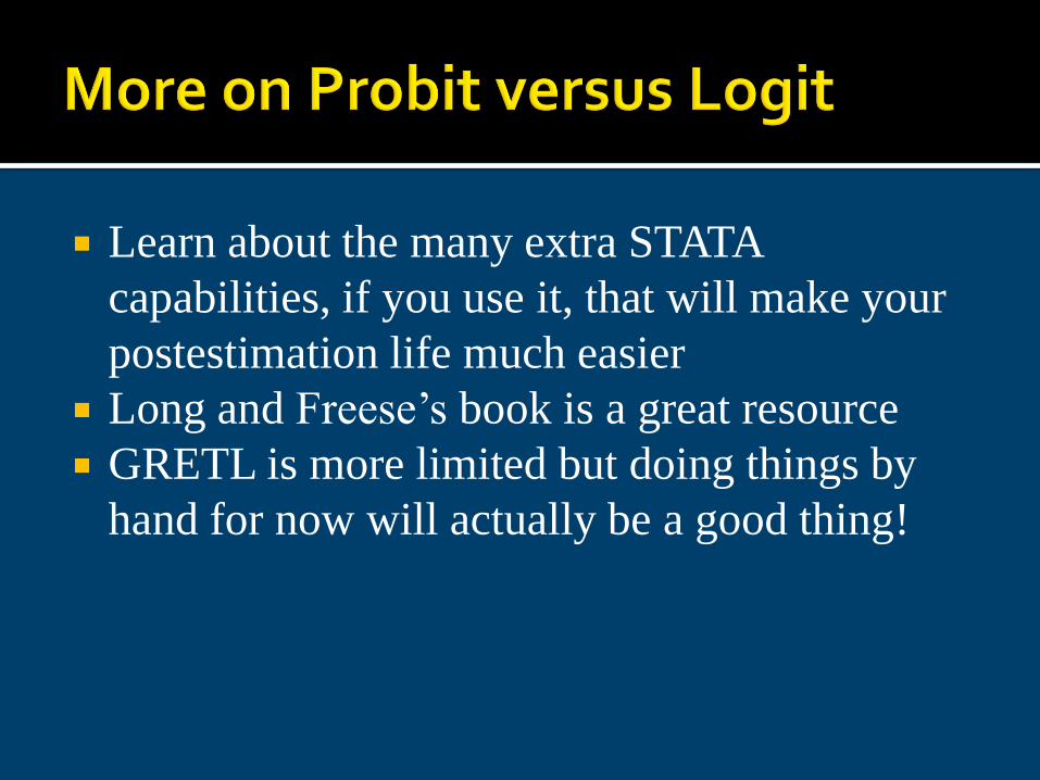
Learn about the many extra STATA
capabilities, if you use it, that will make your
postestimation life much easier
Long and Freese’s book is a great resource
GRETL is more limited but doing things by
hand for now will actually be a good thing!

Slide16-47Principles of Econometrics, 3rd Edition
SDofX = standard deviation of X e^bStdX = exp(b*SD of X) = change in odds for SD increase in X e^b = exp(b) = factor change in odds for unit increase in X P>|z| = p-value for z-test z = z-score for test of b=0 b = raw coefficient dtime 0.05311 2.573 0.010 1.0545 20.5426 56.9104 auto b z P>|z| e^b e^bStdX SDofX
Odds of: 1 vs 0
logit (N=21): Factor Change in Odds
. listcoef, help
_cons -.2375754 .7504766 -0.32 0.752 -1.708483 1.233332 dtime .0531098 .0206423 2.57 0.010 .0126517 .093568 auto Coef. Std. Err. z P>|z| [95% Conf. Interval]
Log likelihood = -6.1660422 Pseudo R2 = 0.5757 Prob > chi2 = 0.0000 LR chi2(1) = 16.73Logistic regression Number of obs = 21
. logit auto dtime, nolog
For example
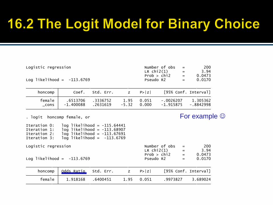
Slide16-48Principles of Econometrics, 3rd Edition
For example
female 1.918168 .6400451 1.95 0.051 .9973827 3.689024 honcomp Odds Ratio Std. Err. z P>|z| [95% Conf. Interval]
Log likelihood = -113.6769 Pseudo R2 = 0.0170 Prob > chi2 = 0.0473 LR chi2(1) = 3.94Logistic regression Number of obs = 200
Iteration 3: log likelihood = -113.6769 Iteration 2: log likelihood = -113.67691 Iteration 1: log likelihood = -113.68907 Iteration 0: log likelihood = -115.64441
. logit honcomp female, or
_cons -1.400088 .2631619 -5.32 0.000 -1.915875 -.8842998 female .6513706 .3336752 1.95 0.051 -.0026207 1.305362 honcomp Coef. Std. Err. z P>|z| [95% Conf. Interval]
Log likelihood = -113.6769 Pseudo R2 = 0.0170 Prob > chi2 = 0.0473 LR chi2(1) = 3.94Logistic regression Number of obs = 200

Stata users? Go through a couple of examples
available online with your own STATA session
connected to the internet. Examples: http://www.ats.ucla.edu/stat/stata/dae/probit.htm http://www.ats.ucla.edu/stat/stata/dae/logit.htm
http://www.ats.ucla.edu/stat/stata/output/old/lognoframe.htm http://www.ats.ucla.edu/stat/stata/output/stata_logistic.htm
Slide 16-50Principles of Econometrics, 3rd Edition
binary choice models censored data conditional logit count data models feasible generalized least squares Heckit identification problem independence of irrelevant
alternatives (IIA) index models individual and alternative specific
variables individual specific variables latent variables likelihood function limited dependent variables linear probability model
logistic random variable logit log-likelihood function marginal effect maximum likelihood estimation multinomial choice models multinomial logit odds ratio ordered choice models ordered probit ordinal variables Poisson random variable Poisson regression model probit selection bias tobit model truncated data

Long, S. and J. Freese for all topics (available on Google!)

Multinomial Logit Conditional Logit


