Econ 508B: Lecture 0 Introductory Econometrics Hongyi Liu Washington University in St. Louis July 30, 2019 Hongyi Liu (Washington University in St. Louis) Math Camp 2018 Stats July 30, 2019 1 / 37
Transcript
Econ 508B: Lecture 0Introductory Econometrics
Hongyi Liu
Washington University in St. Louis
July 30, 2019
Hongyi Liu (Washington University in St. Louis) Math Camp 2018 Stats July 30, 2019 1 / 37
Outline
1 Conditional Expectation and Projection
2 The Algebra of Least Squares
3 Least Squares Regression
4 Time Series Regression
5 Endogeneity (IV)
6 Correlation v.s. Causal effect
7 Large Sample Asymptotics
8 Panel Data Model
9 Machine Learning
Hongyi Liu (Washington University in St. Louis) Math Camp 2018 Stats July 30, 2019 2 / 37
Outline
1 Conditional Expectation and Projection
2 The Algebra of Least Squares
3 Least Squares Regression
4 Time Series Regression
5 Endogeneity (IV)
6 Correlation v.s. Causal effect
7 Large Sample Asymptotics
8 Panel Data Model
9 Machine Learning
Hongyi Liu (Washington University in St. Louis) Math Camp 2018 Stats July 30, 2019 3 / 37
Conditional Expectation
Example 1.1 (wage discrimination)
E (log(wage)|sex = man) = 3.05
E (log(wage)|sex = women) = 2.81
In general,
Definition 1.1 (The specification of Regression Models)
E (y |X) = Xβ + E (u|X) = Xβ
Hongyi Liu (Washington University in St. Louis) Math Camp 2018 Stats July 30, 2019 4 / 37
General Principles
Specification
nonparametric model v.s. parametric model
Information sets
interested in a set of potential explanatory variables
exogenous v.s. endogenous
many explanatory variables? ==> high dimensionality ==> machinelearning
multi-collinearinarity.
Error terms
i.i.d.
serial correlation
heteroskedasticity
Hongyi Liu (Washington University in St. Louis) Math Camp 2018 Stats July 30, 2019 5 / 37
Law of Iterated Expectations E (y |x) = m(x)
Theorem 1.1 (simple version)
If E |y | <∞ then for any random vector x,
E (E (y |x)) = E (y)
Theorem 1.2 (Law of Iterated Expectations)
If E |y | <∞ then for any random vector x1 and x2,
E (E (y |x1, x2)|x1) = E (y |x1)
Theorem 1.3 (Conditioning Theorem)
If E |y | <∞ thenE (g(x)y |x) = g(x)E (y |x)
Hongyi Liu (Washington University in St. Louis) Math Camp 2018 Stats July 30, 2019 6 / 37
Motivation: Best Predictor
Theorem 1.4 (Conditional Mean as Best Predictor)
If E (y2) <∞ then for any predictor g(x),
E ((y − g(x))2) ≥ E ((y −m(x))2)
where E (y |x) = m(x).
Proof.
why the best predicotr is projecton?
Hongyi Liu (Washington University in St. Louis) Math Camp 2018 Stats July 30, 2019 7 / 37
Outline
1 Conditional Expectation and Projection
2 The Algebra of Least Squares
3 Least Squares Regression
4 Time Series Regression
5 Endogeneity (IV)
6 Correlation v.s. Causal effect
7 Large Sample Asymptotics
8 Panel Data Model
9 Machine Learning
Hongyi Liu (Washington University in St. Louis) Math Camp 2018 Stats July 30, 2019 8 / 37
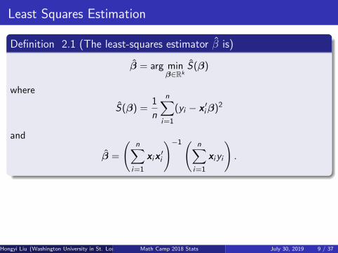
Least Squares Estimation
Definition 2.1 (The least-squares estimator β is)
β = arg minβ∈Rk
S(β)
where
S(β) =1
n
n∑i=1
(yi − x ′iβ)2
and
β =
(n∑
i=1
xix ′i
)−1( n∑i=1
xiyi
).
sketch proof(FOC):
SSE (β) =n∑
i=1
y2i − 2β′n∑
i=1
xiyi + β′n∑
i=1
xix ′iβ
Hongyi Liu (Washington University in St. Louis) Math Camp 2018 Stats July 30, 2019 9 / 37
The sample moment estimator
Why do we need to consider moment estimator?
Qxy =1
n
n∑i=1
xiyi
Qxx =1
n
n∑i=1
xix ′i
The moment estimator of β is
β = Q−1xx Qxy
=(1
n
n∑i=1
xix ′i)−1(1
n
n∑i=1
xiyi)
=
(n∑
i=1
xix ′i
)−1( n∑i=1
xiyi
).
Hongyi Liu (Washington University in St. Louis) Math Camp 2018 Stats July 30, 2019 10 / 37
Least Squares Residuals
The fitted value:yi = x ′i β
The residual:ei = yi − yi = yi − x ′i β
Least square trivally implies that:
n∑i=1
xi ei = 0
why?
Hongyi Liu (Washington University in St. Louis) Math Camp 2018 Stats July 30, 2019 11 / 37
Least Squares Residuals
The fitted value:yi = x ′i β
The residual:ei = yi − yi = yi − x ′i β
Least square trivally implies that:
n∑i=1
xi ei = 0
why?
Hongyi Liu (Washington University in St. Louis) Math Camp 2018 Stats July 30, 2019 11 / 37
Matrix notation
y1 = x ′1β + e1
y2 = x ′2β + e2...
yn = x ′nβ + en
And define
y =
y1y2...yn
X =
x ′1x ′2...x ′n
e =
e1e2...en
Hongyi Liu (Washington University in St. Louis) Math Camp 2018 Stats July 30, 2019 12 / 37
Matrix expressions for OLS
y = Xβ + e
β = (X ′X )−1(X ′y)
e = y − X β,Xe = 0
Projection MatrixP = X(X ′X)−1X ′
symmetric: P ′ = P and idempotent: PP = P.
trP = k .
Annihilator MatrixM = In − P
symmetric: M ′ = M and idempotent: MM = M.
trM = n − k .
Hongyi Liu (Washington University in St. Louis) Math Camp 2018 Stats July 30, 2019 13 / 37
Matrix expressions for OLS
y = Xβ + e
β = (X ′X )−1(X ′y)
e = y − X β,Xe = 0
Projection MatrixP = X(X ′X)−1X ′
symmetric: P ′ = P and idempotent: PP = P.
trP = k .
Annihilator MatrixM = In − P
symmetric: M ′ = M and idempotent: MM = M.
trM = n − k .Hongyi Liu (Washington University in St. Louis) Math Camp 2018 Stats July 30, 2019 13 / 37
Estimation of error variance
σ2 = E(e2i )
σ2 =1
n
n∑i=1
e2i = n−1e ′e
σ2 =1
n
n∑i=1
e2i = n−1e ′Me
ANOVA:
y = Py + My = y + ey ′y = y ′y + e′e
(y − 1y)′(y − 1y) = (y − 1y)′(y − 1y) + e′e
Hongyi Liu (Washington University in St. Louis) Math Camp 2018 Stats July 30, 2019 14 / 37
Outline
1 Conditional Expectation and Projection
2 The Algebra of Least Squares
3 Least Squares Regression
4 Time Series Regression
5 Endogeneity (IV)
6 Correlation v.s. Causal effect
7 Large Sample Asymptotics
8 Panel Data Model
9 Machine Learning
Hongyi Liu (Washington University in St. Louis) Math Camp 2018 Stats July 30, 2019 15 / 37
Linear regression model
Definition 3.1 (unbiased estimator)
An estimator θ for θ is unbiased if E(θ) = θ.
Assumption 3.1 (Linear Regression Model)
The obs satisfies the following assumptions:
yi = x ′i β + ei
E(ei |xi ) = 0.
E(y2i ) <∞,E||xi ||2 <∞
and an invertible design matrix
Qxx = E(xix ′i ) > 0.
Hongyi Liu (Washington University in St. Louis) Math Camp 2018 Stats July 30, 2019 16 / 37
E(e2i |xi ) = σ2(xi ) = σ2i
Assumption 3.2 (Homoskedastic Linear Regression Model)
E(e2i |xi ) = σ2(xi ) = σ2
is independent of xi .
Theorem 3.1 (Mean of Least-Squares Estimator)
In the linear regression model and i.i.d. sampling
E(β|X ) = β
Hongyi Liu (Washington University in St. Louis) Math Camp 2018 Stats July 30, 2019 17 / 37
Variance of Least Squares Estimator
D = diag(σ21, . . . , σ2n)
Theorem 3.2 (Variance of Least-Squares Estimator)
In the linear regression model and i.i.d. sampling
Vβ = var(β|X
)= (X ′X)−1(X ′DX)(X ′X)−1
In the homoskedastic linear regression model and i.i.d. sampling
Vβ = σ2(X ′X )−1
Theorem 3.3 (Gauss-Markov Theorem)
In the homoskedastic linear regression model and i.i.d. sampling, if β is alinear unbiased estimator of β then var(β|X ) ≥ σ2(X ′X )−1.
Hongyi Liu (Washington University in St. Louis) Math Camp 2018 Stats July 30, 2019 18 / 37
Outline
1 Conditional Expectation and Projection
2 The Algebra of Least Squares
3 Least Squares Regression
4 Time Series Regression
5 Endogeneity (IV)
6 Correlation v.s. Causal effect
7 Large Sample Asymptotics
8 Panel Data Model
9 Machine Learning
Hongyi Liu (Washington University in St. Louis) Math Camp 2018 Stats July 30, 2019 19 / 37
Stationarity and Ergodicity
Definition 4.1
{yt} is covariance (weakly) stationary if
E(yt) = µ
is independent of t, and
cov(yt , yt−k) = γ(k)
is independent of t for all k . γ(k) is called the autocovariance function.
ρ = γ(k)/γ(0) = corr(yt , yt−k)
is the autocorrelation function.
Hongyi Liu (Washington University in St. Louis) Math Camp 2018 Stats July 30, 2019 20 / 37
Definition 4.2
{yt} is strictly stationary if the joint distribution of (yt , ..., yt−k) isindependent of t for all k .
Definition 4.3
A stationary time series is ergodic if γ(k)→ 0 as k →∞.
Hongyi Liu (Washington University in St. Louis) Math Camp 2018 Stats July 30, 2019 21 / 37
Outline
1 Conditional Expectation and Projection
2 The Algebra of Least Squares
3 Least Squares Regression
4 Time Series Regression
5 Endogeneity (IV)
6 Correlation v.s. Causal effect
7 Large Sample Asymptotics
8 Panel Data Model
9 Machine Learning
Hongyi Liu (Washington University in St. Louis) Math Camp 2018 Stats July 30, 2019 22 / 37
Endogeneity Bias
Example 5.1 (Demand and supply)
qdi = α0 + α1pi + ui , (demand equation)
qsi = β0 + β1pi + vi , (supply equation)
qdi = qsi , (market equilibrium)
solve for (pi , qi ) as
pi =β0 − α0
α1 − β1+νi − µiα1 − β1
qi =α1β0 − α0β1α1 − β1
+α1νi − β1µiα1 − β1
The OLS estimators are trivially inconsistent!!!
Hongyi Liu (Washington University in St. Louis) Math Camp 2018 Stats July 30, 2019 23 / 37
Instrumental variable
Two conditions for IV, eg. xi , yi :
informative condition: cov(xi , pi ) 6= 0.
validation condition: cov(xi , µi ) = 0
IV estimator is also referred to as two-stage least squares (2SLS). Why?
Z −−−−−−→ X −−−−−−→ Yx ↗
u
Question?
what if the number of endogenous variables is greater one?
what if #(IV) > or < #(endogenous vars)
Hongyi Liu (Washington University in St. Louis) Math Camp 2018 Stats July 30, 2019 24 / 37
Outline
1 Conditional Expectation and Projection
2 The Algebra of Least Squares
3 Least Squares Regression
4 Time Series Regression
5 Endogeneity (IV)
6 Correlation v.s. Causal effect
7 Large Sample Asymptotics
8 Panel Data Model
9 Machine Learning
Hongyi Liu (Washington University in St. Louis) Math Camp 2018 Stats July 30, 2019 25 / 37
Why do we care about the estimator of the β?
y = Xβ + e
Often we say that beta is the effect of a one unit change in x on y.
Can we say that one-unit change in x causes beta-unit change in y?
Regression alone can only establish the correlation or associationbetween two variables.
Hongyi Liu (Washington University in St. Louis) Math Camp 2018 Stats July 30, 2019 26 / 37
Hongyi Liu (Washington University in St. Louis) Math Camp 2018 Stats July 30, 2019 27 / 37
Correlation v.s. Causal effect
Question: How to capture the casual effect?
Example 6.1
a potential outcome function:
y(x1) = h(x1, x2,µ)
Consider x1 is a binary variable, such a medical treatment. Then thecasual effect will be characterized by
C (x2, µ) = y(1)− y(0) = h(1, x2, µ)− h(0, x2, µ)
Hongyi Liu (Washington University in St. Louis) Math Camp 2018 Stats July 30, 2019 28 / 37
Outline
1 Conditional Expectation and Projection
2 The Algebra of Least Squares
3 Least Squares Regression
4 Time Series Regression
5 Endogeneity (IV)
6 Correlation v.s. Causal effect
7 Large Sample Asymptotics
8 Panel Data Model
9 Machine Learning
Hongyi Liu (Washington University in St. Louis) Math Camp 2018 Stats July 30, 2019 29 / 37
Convergence in Probability
A random variable Xn ∈ R converges in probability to X as n→∞,denoted Xn
p−→ X , if for all δ > 0,
limn→∞
P(|Xn − X | ≤ δ) = 1
Theorem 7.1 (Weak Law of Large Numbers)
If yi are i.i.d and E|y | <∞, then as n→∞,
y =1
n
n∑i=1
yip−→ E(y).
Definition 7.1
consistency An estimator θ of a parameter θ is consistent if θp−→ θ.
Hongyi Liu (Washington University in St. Louis) Math Camp 2018 Stats July 30, 2019 30 / 37
Outline
1 Conditional Expectation and Projection
2 The Algebra of Least Squares
3 Least Squares Regression
4 Time Series Regression
5 Endogeneity (IV)
6 Correlation v.s. Causal effect
7 Large Sample Asymptotics
8 Panel Data Model
9 Machine Learning
Hongyi Liu (Washington University in St. Louis) Math Camp 2018 Stats July 30, 2019 31 / 37
Fixed effects and random effects model
Static Panel Data Model:
yit = x ′itβ + µi + eit .
random effects model: E(x ′itµi ) = 0.
fixed effects model: E(x ′itµi ) 6= 0.
Estimation methods: LSDV, First difference, Between estimator,etc
A dynamic panel regression:
yit = αyi ,t−1 + x ′itβ + µi + eit .
Hongyi Liu (Washington University in St. Louis) Math Camp 2018 Stats July 30, 2019 32 / 37
Outline
1 Conditional Expectation and Projection
2 The Algebra of Least Squares
3 Least Squares Regression
4 Time Series Regression
5 Endogeneity (IV)
6 Correlation v.s. Causal effect
7 Large Sample Asymptotics
8 Panel Data Model
9 Machine Learning
Hongyi Liu (Washington University in St. Louis) Math Camp 2018 Stats July 30, 2019 33 / 37
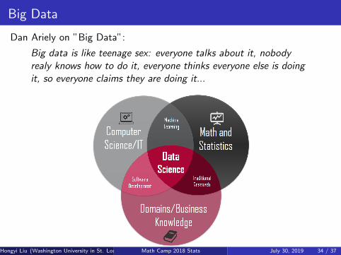
Big Data
Dan Ariely on ”Big Data”:
Big data is like teenage sex: everyone talks about it, nobodyrealy knows how to do it, everyone thinks everyone else is doingit, so everyone claims they are doing it...
Hongyi Liu (Washington University in St. Louis) Math Camp 2018 Stats July 30, 2019 34 / 37
Big Data
Dan Ariely on ”Big Data”:
Big data is like teenage sex: everyone talks about it, nobodyrealy knows how to do it, everyone thinks everyone else is doingit, so everyone claims they are doing it...
Hongyi Liu (Washington University in St. Louis) Math Camp 2018 Stats July 30, 2019 34 / 37
Big Data
Dan Ariely on ”Big Data”:
Big data is like teenage sex: everyone talks about it, nobodyrealy knows how to do it, everyone thinks everyone else is doingit, so everyone claims they are doing it...
Hongyi Liu (Washington University in St. Louis) Math Camp 2018 Stats July 30, 2019 34 / 37
Machine learning
Goal: find a model that is flexible enough to accommodate importantpatterns but not so flexible that it overspecializes to specific data set
All modern methods concern with high dimensional models: Nobservations, P parameters, and N ≈ P or N � P.
Supervvised learning
Want to predict target variable Y with input variables X .AKA: ”predictive analytics”
Unsupervised learning
Want to find structure within set of variables XAKA: ”exploratory data analysis”, ”fancy descriptive statistic”
Hongyi Liu (Washington University in St. Louis) Math Camp 2018 Stats July 30, 2019 35 / 37
Model Selection
Two reasons OLS may be unsatisfactory:
Estimates tend to have low bias but large variance.
Model interpretation: we may want small subset with strongesteffects and are willing to sacrifice small details.
These considerations motivate selecting small model that includes only asubset of predictors.
Hongyi Liu (Washington University in St. Louis) Math Camp 2018 Stats July 30, 2019 36 / 37
Model Selection
General idea:
Search across all permutations of models
Choose best model according to some criterion
Challenages:
Set of models may large
Best model of size k , for k = 1, ..,N
Combinations are∑
k≤N
(Nk
)= 2N .
Which criterion?
Hongyi Liu (Washington University in St. Louis) Math Camp 2018 Stats July 30, 2019 37 / 37