Econ101 PAID IJBEL formattedThe Impact of Cyclical Factors ...

International Journal of Business, Economics and Law, Vol. 6, Issue 3 (Apr.)

ISSN 2289-1552 2015

28

THE IMPACT OF CYCLICAL FACTORS ON THE U. S. BALANCE OF PAYMENTS Magda Kandil

Joshua Greene

ABSTRACT

Real GDP growth and real effective exchange rate (REER) appreciation appear co-integrated with the current and financial

accounts of the U.S. balance of payments. On this basis, we estimate reduced form equations showing that expected changes and

shocks to real GDP, the REER, energy prices, and growth in emerging market economies and other industrial countries explain

much of the short-term variation in the U.S. current account balance, with the balance worsening as real GDP, the REER, and to a

lesser extent, energy prices increase. In addition, the financial balance improves with real growth and an increase in the oil price,

while stock market prices affect the composition of capital inflows.

JEL Classification Numbers: F3; F4

Keywords: United States; balance of payments; current account; capital and financial account

I. INTRODUCTION*

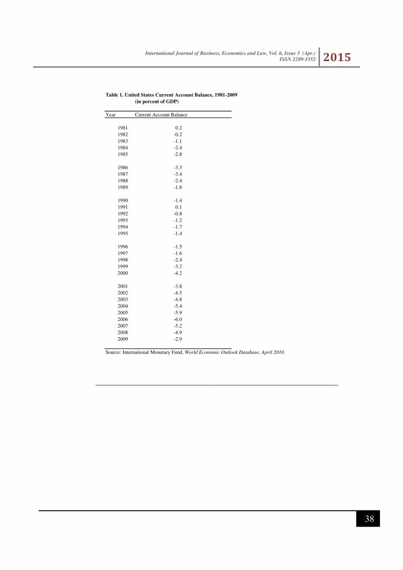
The United States has experienced current account deficits exceeding 1 percent of GDP during all but two of the years since 1981

(Table 1). In 2000, the current account deficit reached 4.2 percent of GDP. Although it declined in 2001 to 3.8 percent of GDP,

reflecting the economic slowdown, the ratio has since increased to 4.5 percent in 2002, 4.8 percent in 2003, and even higher deficit to

GDP in 2004, 5.4 percent. More recently, the current account balance in the U.S. further deteriorated in the period leading to the

global financial crisis. The sustainability of the widening deficit in the current account deficit was a function of financial inflows to

the United States. Major trading partners, led by China, took interest in financing the widening deficit in the United States to sustain

American imports of their products as they sought to depreciate their domestic currencies relative to the US dollar to maintain export

competitiveness. Other partners, particularly oil producing countries, have sought financial investments in the United States to

mobilize the increased wealth of financial resources that have become available, beyond their absorptive capacity, as the oil price

continued to surge. Under both scenarios, strong fundamentals of the US economy have attracted interest for growing financial

investments in the United States that enabled sustainability of a widening current account deficit.

The global financial crisis has drawn attention to problems attached to global imbalances attributed to the above scenario. While the

United States enjoyed growing and spending beyond its domestic resources, excessive leveraging and financing had adverse global

effects in the absence of adequate prudential oversight to ensure sustainability of financing. In the aftermath of the global crisis, all

partners, particular major global powers, have agreed that restructuring is necessary to sustain global demand going forward. At the

core of this restructuring agenda is the need for trading partners to reconsider their external balances. The United States cannot

maintain excessive current account deficit financed by external sources. Hence, there is a need to contain domestic spending and

mobilize export demand. On the other hand, countries like China would need to mobilize domestic spending to continue to grow

without excessive dependency on export orientation, particularly in one or a few major partners. Indeed, in the aftermath of the

global financial crisis both sides have stepped up efforts for restricting their economies along these directions. More recently, ending

quantitative easing of monetary policy in the U.S. presents a real risk of a slowdown in emerging markets that could risk the

momentum of sustaining global growth and require further coordination of policies to address associated imbalances, both domestic

and external.

To inform the economic agenda of restructuring and reflect on the type of imbalances leading to the global financial crisis, the

research of this paper aims at taking a closer look at the current account deficit in the United States and sources of financing. As

researchers drew attention to concerns about inadequate sources of sustainability, some projections in the early part of the last decade

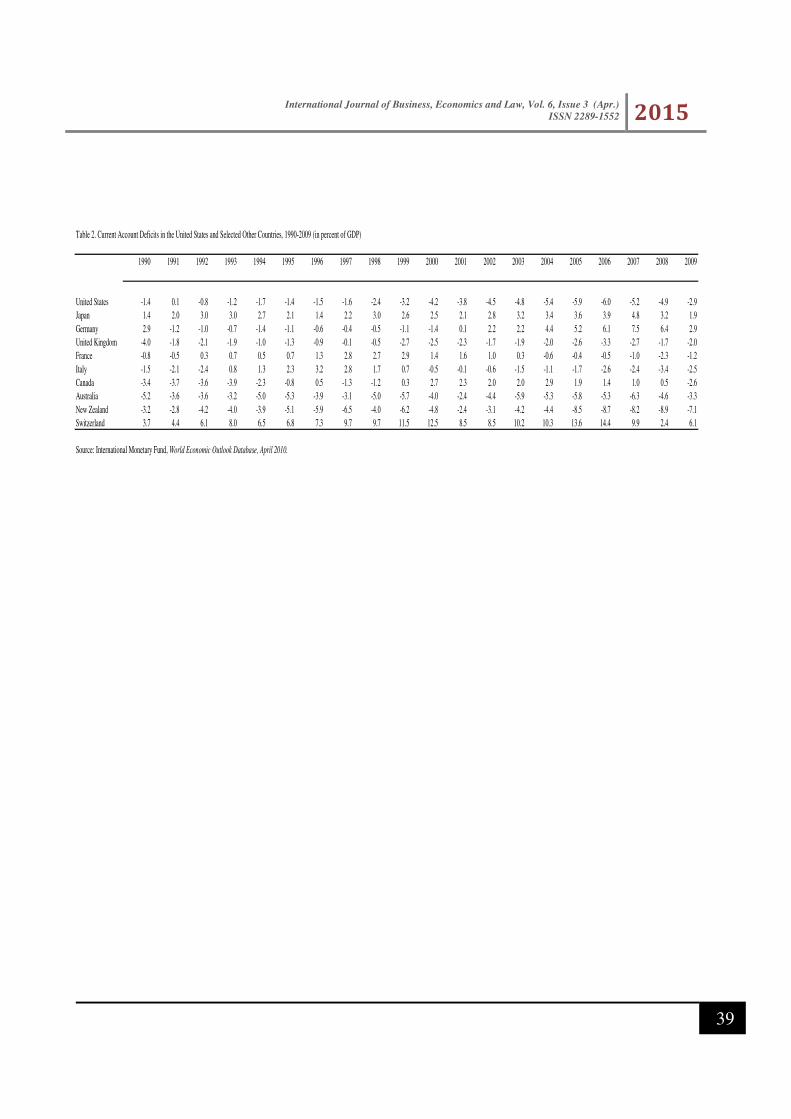
(Mann, 2001) showed the current account deficit averaging above 4.5 percent. Although these levels are not large compared to those

experienced by some industrial countries, such as Australia and New Zealand, and many developing countries, they are high

compared to the current account balances of the larger industrial countries (Table 2). Thus, questions have arisen about the

sustainability of current account deficits exceeding 4 percent of GDP over the medium to long term in the sense of Milesi-Ferretti and


ISSN 2289-1552 2015

29

Razin (1996), meaning that they can be maintained without the need for drastic changes in domestic macroeconomic policy.1 For

example, Obstfeld and Rogoff (2000), writing before the start of the 2001 recession in the United States, argued that the U.S. current

account balance was quite likely to reverse by 2010, predicting that a rapid adjustment could lead to a real depreciation of the dollar

by more than 20 percent.2

Contemporary economic theory views current account sustainability as a medium-term issue, turning on the ability of countries to

generate sufficient current account surpluses in future years to offset present deficits (Chinn and Prasad, 2000; Debelle and Faruquee,

2000; and Arora, Dunaway, and Faruquee, 2001). More recently, the liberalization of capital flows has broadened the scope of

current account sustainability to include the ability to generate a stable and sustainable external net foreign asset position to finance a

widening current account deficit over time. Nevertheless, economists have found that the current account position of industrial

countries varies with the state of the business cycle. Faruqee and Debelle (1996), for example, have observed that the business cycle,

as measured by the output gap and the real exchange rate, had significant short-term effects on the current account balance for a

number of industrial countries during the 1971–93 periods. Freund (2000) has noted that, in industrial countries, a common pattern

during the 1980–97 periods was for the current account deficit to begin reversing after reaching a level of about 5 percent of GDP and

to continue improving over a period of several years.

Data for the United States also suggest a strong cyclical influence on the balance of payments. As Chart 1 indicates, the current

account balance has often recorded surpluses during recessions, such as 1974–75, 1980, and 1991, and deficits during periods of

strong economic growth (e.g., 1994–99). However, the relationship is not exact, since some boom years (e.g., 1973) have recorded

surpluses, while some recession years (e.g., 1982) have recorded deficits. Similarly, the financial account of the balance of payments

and foreign direct investment has also varied over the business cycle. For example, both grew strongly during the last half of the

1990s, when U.S. economic growth began to exceed that of other industrial countries, arguably triggering capital inflows to the

United States.

Because cyclical factors seem to have a major impact on the US balance of payments, it seems worthwhile analyzing the effect of

these variables in a more systematic way.3 This includes studying the impact of these variables not only on the external current

account, but also on the capital and financial accounts, which have been instrumental in financing the country’s large current account

deficits. This may be consistent with the lower capital-output ratios and higher returns to capital observed in the United States than in

most other industrial countries during the last half of the 1990s (see Arora, Dunaway, and Faruqee, 2001; Cooper, 2001, and

McKinnon, 2001). Since the growth in productivity often mirrors business cycles, analysis may show that cyclical factors also have

an impact on the capital and financial accounts of the balance of payments.

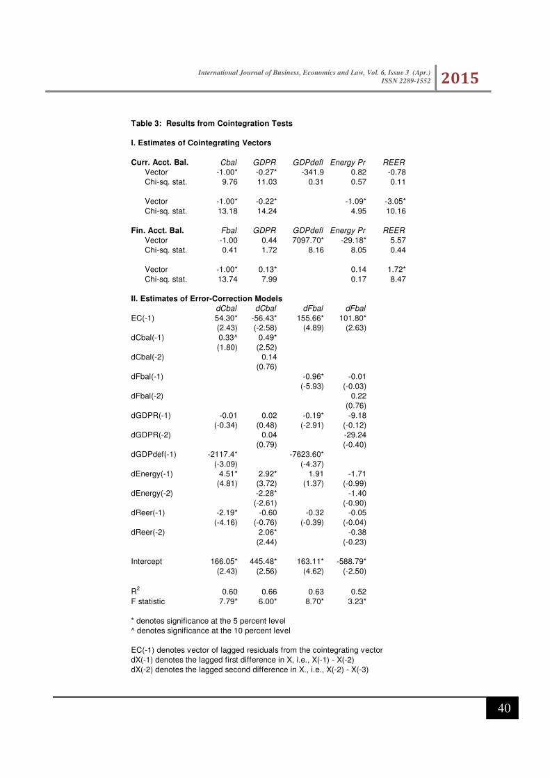
This paper follows a two-step procedure. First, co-integration analysis is used to confirm that cyclical factors bear a long-term

relationship to the current account and the financial account (the main element of the capital and financial account) of the U.S.

balance of payments. Second, the paper estimates a series of reduced form equations in differenced form, using annual data, for the

current account balance, the financial account balance, and important components of each balance, using a number of macroeconomic

indicators reflecting the state of the business cycle as explanatory variables. These include not only a measure of economic growth,

but also other factors that vary cyclically, such as inflation, energy prices, and returns on financial assets. In addition, following work

by Kandil (2000) on other macroeconomic indicators, the paper examines the effect of positive and negative shocks to these and other

cyclical variables on components of the balance of payments.

To anticipate the results, the empirical work confirms that cyclical factors have a significant impact on the current account balance,

with higher real growth, a more appreciated real exchange rate, and higher energy prices having the expected negative impact on the

current account balance.4 In addition, shocks to certain variables have asymmetric effects on the current account balance. Co-

1 The IMF’s Executive Board, for example, questioned the sustainability of the U.S. external current account deficit over the longer

term during the IMF’s 2001 Article IV Consultation with the United States (International Monetary Fund, 2001b). Subsequently, the

IMF has raised concerns about the deficit as part of a broader concern over global macroeconomic imbalances that threaten world

prosperity (see, for example, International Monetary Fund, 2005).

2 Between 2001 and 2004, the dollar depreciated relative to the euro by 24 percent, in real terms, and by 27.5 percent, in nominal

terms. More recently, the United States has been pursuing a quantitative easing policy to stimulate the economy and depreciate the

US dollar with an aim to mobilize exports, which has been reversed in the context of the Fed’s recent announcement of tapering its

expansionary stance till it ended the quantitative easing program in November 2014.

3 For related literature, see Cheung, Funceri and Rusticelli (2010).

4 The positive relationship between key variables and the financial balance could result to cover deficits in the current account. The

positive relationships could reflect the need for the financial balance to offset movements in the current account, since reserves are

finite.


ISSN 2289-1552 2015

30

integration indicates a negative long-term relationship between the current account and each of real GDP, the real effective exchange

rate and the oil price. Consistently, there is a positive long-term relationship between the financial account balance and each of real

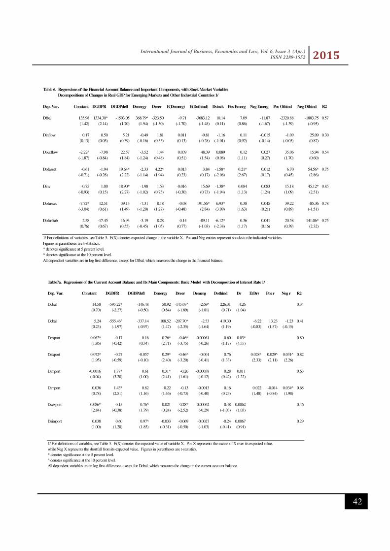
GDP, the real exchange rate, and the oil price. In addition, reduced form equations suggest that domestic real GDP growth and oil

price inflation are important factors that support improvement in the financial balance in the U.S. The composition of net financial

flows between various financial assets is highly dependent on variation in stock prices in the U.S.

The rest of the paper is organized as follows. Following a theoretical discussion of the models in section II, section III reports the co-

integration analysis of the current and financial accounts. Section IV reports the results of the reduced form equations. Section V

summarizes the main findings in the paper.

II. MODELING CYCLICAL EFFECTS ON THE U. S. BALANCE OF PAYMENTS

The literature suggests that the main components of the balance of payments, in particular the current account balance, are sensitive

to cyclical economic factors. To test this hypothesis, we use the following procedure. First, we test for cointegration between key

cyclical factors and the main elements of the balance of payments, to examine the long-term correlations between these two sets of

variables. Next, we estimate a series of reduced form equations relating the current account balance, its main components, and the

main components of the capital and financial account balance to a series of macroeconomic variables that are cyclically sensitive. To

track business cycles, these models are estimated on a short-term basis. Because data on foreign economic growth are available only

on an annual basis, and the results are stronger, we prefer models based on annual data, although we also examine models using

quarterly data.

Equations are estimated both for the current and financial account balances and their main components. As explanatory variables, we

use cyclically sensitive macroeconomic indicators reflecting the following analysis.

A. Procedures, Variables, and Data

To examine the different hypotheses regarding the current and the capital and financial accounts, reduced form equations were

estimated for both the aggregate balances and for important components of each account.

For the current account, equations were estimated for the current account balance, exports and imports of goods, and exports and

imports of services. For the capital and financial account, equations were estimated for the financial account balance, total financial

inflows, total financial outflows, total inflows by foreign parties other than governments, inflows for foreign direct investment,

inflows for holdings of government securities, inflows for holdings of non-government securities, and inflows for liabilities of banks

and other financial institutions, the latter representing mostly accumulations of deposits and certificates of deposit at U.S. banks.

Because amounts in the capital account were small, no equations were estimated for the combined capital and financial account.5

Tests (see, for example, Dickey (1976), Fuller (1976), and Nelson and Plosser (1982)), which included both a constant and a time

trend, indicated that the external sector balances and the different explanatory variables had unit roots in levels but not in first

differences, so the equations were estimated using first differences6. Because the current and financial account balances could take

negative values, they were estimated as changes in levels. The components of these balances were estimated as changes in

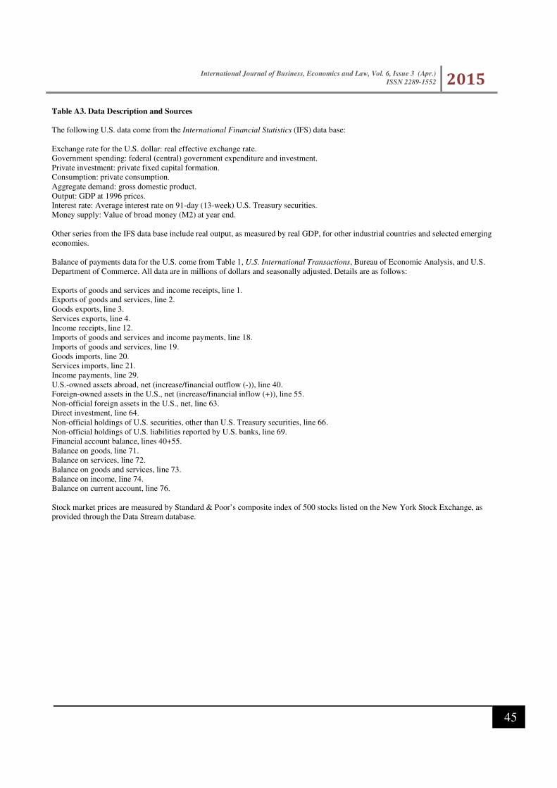
logarithms, however. A list of the dependent variables and data sources appear in Appendix I.7

To isolate the effects of key variables, a basic set of reduced form equations was estimated using the changes in the following as

explanatory variables: real GDP, the GDP deflator, an index of energy prices, the real effective exchange rate of the U.S. dollar, and

5 In the US balance of payments, the capital account includes estimates of debt forgiveness by the U.S. government, transfers of

assets by immigrants to the United States (comparable transfers by emigrants are excluded, because of insufficient data), and sales

and acquisitions of some nonproduced, nonfinancial assets (transactions in natural resources and a few large transactions in other

types of such assets). See IMF (2001a, p. 365). Because the relevant items are small, the capital account in the U.S. balance of

payments is also small.

6 Tests were conducted for the null hypothesis of non-stationarity and proved robust, using the test suggested by Kwiatkowki et al.

(1992) for the null hypothesis of stationarity. Results are available upon request.

7 For the financial account, we consider data for inflows and outflows, net. Given our interest to explain cyclicality in financial

inflows, which are necessary to finance the current account deficit, we consider several types of inflows, as listed in Appendix I.


ISSN 2289-1552 2015

31

weighted averages of real GDP in emerging market economies and of industrial countries other than the United States.8 9 10 To

illustrate asymmetries in the effects of positive and negative shocks to individual variables, actual changes for certain variables were

replaced by expected values and positive and negative shocks. The technique for deriving expected changes in variables is described

in Appendix II. Positive and negative shocks were calculated as the excess or shortfall of actual from expected values of the variables.

One benefit from examining separately the impact of macroeconomic shocks and forecastable events on the balance of payments is

that the two phenomena may affect the same variable over different time periods. Shocks are random components of an observed

variable that have, by construction, a zero mean. Thus, they should have only temporary effects on a variable that cancel out over

time. Forecastable events, by comparison, are more likely to have longer lasting effects on a variable. Decomposing a variable into

forecasted and shock elements allow testing whether an observed relationship between two variables reflects mainly temporary, or

also longer lasting, effects. Several equations also tested for the impact of U.S. stock market prices, as measured by Standard &

Poor’s index of 500 stocks listed on the New York Stock Exchange. Appendix I also include a list of the explanatory variables used

in the equations.

The various equations were estimated using both annual and quarterly data, because quarterly data for the relevant variables were not

available for some industrial and many emerging market countries. The annual equations were estimated over the period 1970–2010,

while those with quarterly data were estimated over the 1980–2009 periods and for the 1980-1990, 1990–2000 and 2000–2009

periods, to see if new trends in the data appeared more recently.11 Appendix II describes in detail the econometric methodology. The

sample period ends before the global financial crisis to establish evidence on global imbalances and underlying factors, widely

believed to be a major contributor to the crisis, and establish robust evidence that is not specific to the episode of the crisis.

The annual equations had the following form, sometimes including a stock price variable, with one set of explanatory variables

entered as actual changes (shown below with the subscript “i”) and a second set (shown with the subscript “j”) decomposed into

expected changes and positive and negative shocks (positive and negative differences from the expected changes):

DYt = b0 + Σi,t bi DX i,t + Σj,t cj E(DZj,t) + Σj dj,t PosZj,t + Σj hj,t NegZj,t + ut,

Where:

DYt represents the first difference in one of the dependent variables (the current account balance, financial account balance,

or the log of one of their major components);

8 To determine whether trade liberalization affected the results, the equations were also estimated using dummies for each of the three

major postwar rounds of tariff negotiations—the Kennedy, Tokyo, and Uruguay rounds. Only the Kennedy round dummy (years from

1969 onward) had a significant coefficient in any of the equations, and then only for exports and imports of goods. Accordingly, the

equations reported include no trade round dummies.

9 We relate the nominal values measured in the balance of payments to real variables and price indices (such as changes in real GDP

and in the GDP deflator) rather than just nominal variables (such as nominal GDP), to shed more light on the sources of cyclical

fluctuations in the dependent variables. The real effective exchange rate captures relative competitiveness, as measured by bilateral

movements in the exchange rate and relative CPI inflation with respect to major trading partners.

10 The list of industrial countries includes Australia, Austria, Belgium, Canada, Denmark, Finland, France, Germany, Greece, Iceland,

Ireland, Italy, Japan, Luxembourg, the Netherlands, New Zealand, Norway, Portugal, Spain, Sweden, Switzerland, and the United

Kingdom. The set of emerging market economies was chosen based on data availability and relevance of the U.S. balance of

payments. The economies included are Argentina, Brazil, Chile, Colombia, Cyprus, Hong Kong SAR, Hungary, Israel, Korea,

Mexico, Oman, Saudi Arabia, Singapore, South Africa, Thailand, Turkey, Uruguay, and Venezuela. For both industrial and emerging

market groups, the index was constructed as a geometric weighted average of real output in each economy, such that the log of the

average equals a weighted sum of the log of real output in each economy. The weights were determined by the ratio of each

economy’s output to total output in the group.

11 Regressions with quarterly data were estimated using, as explanatory variables, two- or four-quarter distributed lags of those

variables available on a quarterly basis: changes in real GDP, the GDP deflator, energy prices, and the real effective exchange rate. In

one variant a four-quarter distributed lag of stock market prices was also included. The results of the regressions (available upon

request) differed somewhat, depending on the observation period. In addition, the quarterly regressions for the entire period yielded

somewhat different results from those using annual data. Nevertheless, the broad trends emerging from the quarterly regressions, in

general, confirm those using annual data.


ISSN 2289-1552 2015

32

DX i,t represents the change in the i-th explanatory variable X, entered as a difference in its actual value from the previous

year, without decomposition;

E(DZj,t) represents the expected value of the change in the decomposed j-th explanatory variable Z;

PosZj,t represents positive shocks to the j-th explanatory variable Z;

NegZj,t represents negative shocks to the j-th explanatory variable Z; and ut is a disturbance term.12

Depending on the equation, one or more sets of explanatory variables were decomposed into expected values and positive and

negative shocks from these values. In some versions of the equations the two external variables (EMERG—the index of real GDP in

emerging market economies, and OTHERIND—the index of real GDP in other industrial countries) were decomposed.13 This

specification is the basic model. In others, the four domestic variables (GDPR—real GDP, GDPDEF—the GDP deflator,

ENERGY—the index of energy prices, and REER—the real effective exchange rate of the U.S. dollar) were decomposed.

Before undertaking this analysis, however, the endogeneity of potential explanatory variables must be addressed. The reduced form

equations explaining the current and financial accounts are estimated jointly with equations that approximate agents’ forecasts of

decomposed variables in the model, using three stage least squares (3SLS). Instrumental variables are used to proxy the endogenous

variables in the model, including the real effective exchange rate of the U.S. dollar during the current period (see Appendix II for

details). In this way the problem of simultaneity between certain variables, such as the current account balance and GDP, is

addressed.14 Instruments include the lagged value of the first-difference of the logarithms of real output, the price level, broad money

supply, federal government expenditure, and the real exchange rate of the U.S. dollar.

B. Current Account

Both economic theory and the work of other researchers suggest that the current account of the U.S. balance of payments should be

sensitive to domestic economic conditions. As noted earlier, Freund (2000) has commented that the current account balances of most

industrial countries have responded to changes in real GDP growth rates, with deficits typically widening during the expansionary

part of a business cycle and contracting or becoming surpluses as real GDP growth declines. Thorough discussion of the theory that

links current accounts to the business cycle can be found in Baxter (1995) and Prasad (1999), for example. To summarize, different

types of macroeconomic shocks influence the cyclical dynamics of the trade (current) account balance. The two main determinants of

the trade balance are assumed to be relative output and the real exchange rate. The short-run equilibrium in the presence of sluggish

price adjustment indicates the following. The effects of supply shocks and nominal shocks on the trade balance are ambiguous and

depend, inter alia, on the elasticities of the trade balance with respect to relative output and the real exchange rate. On the other hand,

permanent demand shocks, which result in an appreciation of the real exchange rate concomitantly with a transitory increase in

relative output, produce an unambiguous trade balance response.

Having reviewed existing theoretical modeling, we would expect real growth to have a negative impact on the current account

balance, raising imports of goods and services. Higher inflation should also worsen the current account balance, raising imports and

reducing exports as competitiveness declines. The same should apply to higher energy prices, since the United States is a net energy

importer.15 Various foreign variables should also be expected to affect the current account balance. Higher foreign growth rates

should spur U.S. exports of goods and services, other things being equal. Variables affecting the real prices of tradables should also

12 Co-integration tests indicate that there is a common trend between each of the current account balance and the financial account

balance and selected explanatory variables in the model. Nonetheless, there is no co-integration vector that combines each dependent

variable and all explanatory variables in any of the estimated models. Hence, it was not necessary to account for an error correction

term in the model specification of the reduced-form equations.

13 The introduction of emerging and industrial countries growth proxies are in line with the evidence in Stock and Watson (2009).

14 In the U.S. the sum of exports and imports of goods and nonfactor services only equals about 25 percent of GDP.

15 There are several other cyclical business indicators in economic theory, including the index of consumer confidence, money growth

rates, new orders for plant and equipment, hours of labor in the manufacturing sector, index of industrial production, among others,

that are likely to impact cyclicality in the current account balance and supporting finance. These factors are not modeled explicitly

due to data limitation and insufficient degrees of freedom. However, they are highly correlated with the composite real growth

variable included in the model.


ISSN 2289-1552 2015

33

affect the external current account balance. Thus, the real effective exchange rate of the dollar should have an impact, with a real

appreciation eventually worsening the current account balance (by reducing exports and increasing imports) and a real depreciation

improving it. In the short run, however, if the economy is highly dependent on imports, the effects may be opposite (indicating a “J-

curve” effect of changes in the real effective exchange rate). Interest rates may also affect the current account balance by changing

net interest payments.

Besides these variables, we also examine the effects of shocks to government spending as a way of testing the impact of fiscal policy

on the current account of the balance of payments. To the extent that policy variables affect domestic performance (real growth, price

inflation, the interest rate, and the exchange rate), it would be interesting to study the effect of policy changes on the current account

and its underlying components.

C. The Capital and Financial Account

The impact of cyclical factors on the capital and financial account of the balance of payments may be harder to predict than the

current account, for a variety of reasons. U.S. financial institutions play a key role in providing financing to other countries and

attracting financial investors from other countries. Thus, net financial inflows to the United States also reflect, to a significant degree,

the financial circumstances of other economies. In this connection, a few exogenous factors are often relevant. For example, dollar

assets have historically provided a safe haven for investors seeking to diversify financial assets and hedge against currency

fluctuations. Further, many central banks have historically intervened in the foreign exchange market to buy dollar-dominated assets

in an effort to stem domestic currency appreciation and boost export competitiveness.

Nevertheless, one might expect the capital and financial account to respond positively both to current and expected real economic

growth in the United States. This reflects the importance of both direct investment and financial investments by foreigners from

abroad to the United States. Similarly, the capital and financial account might also depend on real growth in the United States relative

to that in other economies. This could be incorporated by including measures of real GDP growth in other country groups, such as

non-U.S. industrial countries and selected emerging market economies. In addition, the actual and predicted performance of the stock

market in the United States may affect the financial account as higher stock prices may trigger net capital inflows.

Finally, since official reserves and the ability to expand the Fed’s balance sheet are limited, there might be an inverse relationship

between the current account and the capital and financial account, with the latter becoming more positive as the former deteriorates.

One implication might be that net inflows in the capital and financial accounts essentially finance current account deficits. In

addition, an inverse relation could result if capital inflows lead to a real appreciation of the U.S. dollar that worsens the current

account balance.

III. CO-INTEGRATION RESULTS

Before estimating the reduced form equations described above, we tested for co-integration between the main domestic economic

variables and the current and financial account balances. This test indicates whether our cyclical variables bear a long-term

relationship to these key balances. The results are summarized in Table 3.

For both the current and financial account balances, two combinations of variables were tested: one including the current or financial

account balance, real GDP, the real effective exchange rate (REER), the index of energy prices, and the GDP deflator; and one with

the first four of these variables, i.e., excluding the GDP deflator. In the case of the current account balance, chi-square statistics

suggested that only the current account balance and real GDP were co-integrated, with the expected negative relationship, when all

five explanatory variables were included. However, when only the first four variables were included, chi-square statistics indicated

that all four variables belonged in the co-integrating vector, with real GDP, energy prices, and the REER all bearing a negative and

significant relationship with the current account balance. For the financial account balance, the combination with five variables

showed only the GDP deflator and energy prices as co-integrated, with a positive relationship. The test with four variables, however,

showed that the financial account balance, real GDP, and the REER were co-integrated, with real GDP and the REER positively

related to the financial account balance.

As the financial account is the mirror image of the current account, the co-integration results suggest that real GDP, energy prices,

and the REER have a negative long-term relationship with the current account balance, while real GDP, with the energy price and/or

the REER have a positive long-term relationship with the financial account balance. The co-integration results indicate that the

relations between variables are long lasting. Hence, domestic conditions have long-run implications for the current account deficit

and its sustainability. Real GDP growth and dollar appreciation seem necessary for the sustainability of the current account deficit.

The inflow of financial assets to finance the current account deficit, attracted by strong fundamentals, supports real growth and

strengthens the dollar value against the depreciating pressure implied by a widening current account deficit. The significance of the

error correction term indicates the importance of cyclical fluctuations between variables in the short run. Hence, understanding the

relation between the financial and current accounts in the long run requires a thorough investigation of cyclical fluctuations in the

short run.


ISSN 2289-1552 2015

34

IV. RESULTS FROM REDUCED FORM EQUATIONS

A. Basic Model with Decompositions

The basic model includes domestic variables and two indices of output growth in selected emerging markets and other industrial

countries. All domestic variables enter the model in first-difference form. Each index of output growth in other countries is

decomposed into three components: an anticipated growth component, a positive shock, and a negative shock. Results appear in

Table 4, which reports regressions for the balances and key components of the current account.16

Table 4 shows that, in this specification, changes in real GDP and the real effective exchange rate both have negative and significant

coefficients. These results imply that growth in real GDP and a more appreciated real exchange rate correspond to a weaker current

account balance, as expected. Surprisingly, however, positive movements in real GDP in emerging market economies and other

industrial countries do not correspond to a stronger U.S. current account. The coefficients for the expected values of these variables

and positive shocks to them are all negative, although significant only for positive shocks to GDP in emerging economies. That is, the

growth in emerging markets’ output is consistent with an increase in U.S. imports relative to exports. This result may mean that GDP

growth in other economies is less important as a determinant of the U.S. current account balance than real growth or real exchange

rate movements in the United States for these other groups of economies. Most other variables have insignificant effects on the

current account balance.

The equations for exports and imports of goods, and to a lesser extent, exports of services, help explain the results of the equation for

the current account balance. The equations for exports of goods and of services both have negative and significant coefficients for

changes in the real effective exchange rate (DREER), suggesting that an appreciation of the real exchange rate worsens the current

account balance by depressing exports. The equation for imports of goods has a positive and significant coefficient on changes in real

GDP (DGDPR), implying that higher real GDP growth worsens the current account balance by raising imports. Both sets of results

conform to theoretical predictions.17 In general, fluctuations in real GDP growth and the real effective exchange rate seem to be the

primary determinants of cyclical fluctuations in the current account balance of the U.S.

The basic equations, with EMERG and OTHERIND decomposed, do a poor job of explaining the financial account and its most

important components (results are available upon request). Most coefficients are insignificant, and the R2 statistics for the equations

are low. Thus, the macroeconomic variables and decompositions here do little to explain movements in the financial account, which

appear to be mostly random and unsystematic.

Table 5 reports the results of equations for the current account balance and its main components in which the four main domestic

economic variables—GDPR, GDPDEF, ENERGY, and REER—are decomposed, while EMERG and OTHERIND are entered as

changes in “actual” (instrumented) values. We report this specification to demonstrate the robustness of our previous findings with

respect to model specification. Further, we seek to investigate possible asymmetry in the effects of domestic variables on components

of the current and financial accounts. This specification does a better job at explaining variations in the current account balance and

key components.

Compared to the results of Table 4, all the equations in Table 5 have noticeably higher R2 statistics, and many of the new variables are

significant at the 10 percent level or better. In the equation for changes in the current account balance, the expected value of changes

in real GDP has the anticipated negative sign and is again quite significant. This reflects positive and highly significant coefficients

on expected changes in real GDP in the equations for imports of goods and of services. This result is consistent with a long-lasting

effect of domestic real conditions on imports and the current account balance. Positive shocks to real GDP growth in the United

States have a positive significant effect on changes in both exports and imports of goods. In contrast, negative shocks improve the

current account balance significantly. The reduction in imports exceeds that of exports during economic downturns. Thus, there is

clear asymmetry in the effects of fluctuations in real GDP growth on the current account balance of the U.S. While both exports and

imports improve during cyclical upturns, the reduction in imports during downturns improves the current account balance. Overall,

16

Because the current and financial account balances are entered as first differences in levels, coefficients in these regressions cannot

be interpreted as elasticities, unlike the case for the other dependent variables. For illustrative purposes, we also re-estimated these

equations reported in Table 4, including two randomly-chosen error-correction terms: one combines the dependent variable with real

GDP, the GDP deflator, and the energy price; the other combining the dependent variable with the exchange rate, index of output in

other industrial countries, and index of output in selected emerging market countries. Adding these terms improved the fit of several

equations, confirming the robustness of the underlying approach. The results are available upon request. 17

The greater effect of own GDP on U.S. imports than foreign GDP on U.S. exports is the well-known result of Houthakker and

Maggee (1969) that the income elasticity of U.S. import demand is about double the income elasticity of foreign demand for U.S.

goods.


ISSN 2289-1552 2015

35

the results indicate that the inverse relationship between the current account and the business cycle in the U.S. is particularly evident

during recessions.

Table 5 also shows that expected appreciations in the real exchange rate have a negative effect on the current account balance,

consistent with theoretical expectations and the result in Table 4. On the other hand, higher expected energy prices have a positive but

insignificant effect on changes in the current account balance. This is consistent with a significant increase in exports when

anticipated energy prices rise, as the equation for exports of goods suggests. However, positive shocks to energy prices have a

significant negative effect on the current account balance, reflecting a greater impact on imports than on exports. Since the United

States is a net energy importer, higher-than-expected energy prices should coincide with a weaker current account balance. This is

consistent with a larger positive coefficient on imports compared to exports in response to higher-than-expected energy prices. The

quantity demanded of energy imports is inelastic with respect to the rise in prices. Hence, the value of imports is rising. Surprisingly,

unexpectedly low energy prices also worsen the current account, as evident by the positive and statistically significant coefficient.

Both exports and imports behave asymmetrically in the face of energy price shocks. U.S. exports do not decline with the reduction in

energy prices. Moreover, imports do not decrease, despite the reduction in energy prices. There appears to be a tendency for the

quantity of energy imports demanded to rise in response to an unexpected reduction in prices. Further, imports may increase because

lower energy prices are accompanied by higher economic activity.

The model specification in Table 5 also demonstrates that positive changes to real GDP in emerging markets are significantly related

to a weaker current account balance. Higher real GDP growth in other industrial countries is positively and significantly related both

to higher goods exports and to higher goods imports. However, the coefficient in the equation for exports of goods is noticeably

larger than that on imports, suggesting that the main effect of higher growth in other industrial countries is to raise U.S. exports,

despite the results in Table 4.

Estimating the financial balance with the specification that decomposes domestic variables yields no better results. The results are

available on request.

B. Effect of Stock Market Prices

As a way of improving the results for the financial balance, Table 6 reports the effect of adding a variable for U.S. stock market

prices to the previously estimated model. As the equation already accounts for relative growth in the US, compared to major

advanced and emerging countries, we seek to test the performance of the stock market in the US, regardless of developments in other

major stock markets. The stock market variable has a powerful impact on a number of these equations, sharply increasing the R2

statistics, particularly for certain equations in the financial account.18

We analyze data in the financial balance and underlying net flows that determine the stock of foreign holdings of financial assets in

the United States. Table 6 shows changes in the financial balance and underlying changes in net flows of financial assets. The

strongest effects of stock market prices appear in equations for certain components of the financial account, for which the R2 statistics

increase noticeably. Moreover, there is evidence that stock prices affect the composition of net capital flows to the United States.

Adding the stock market variable has a negative effect, significant at the 10 percent level or better, on the change in foreign flows to

hold U.S. official assets, foreign direct investment, and other financial liabilities of the United States. In addition, it has a positive and

highly significant effect on the change in net foreign flows to hold nonofficial U.S. securities, which include stocks.19 Thus, higher

stock prices appear to increase the rate of flows into foreign acquisitions of private U.S. securities at the expense of net flows for

official securities, foreign direct investment, and deposits or certificates of deposit in U.S. financial institutions.

18

Adding the stock market variable to the estimated model for the current account in Table 4 (results are available upon request)

does not affect the impact of changes in real GDP, for which the coefficient remains negative and significant at the five percent level.

The coefficients for the change in stock market prices are negative and significant at the 10 percent level in the export and import

equations. The negative sign in the export equation could reflect the role of higher stock prices in appreciating the real exchange rate,

thus reducing the competitiveness of exports. The negative sign in the import equation may reflect, for example, a shift from

consumption to financial investment activity when stock prices are higher. Mercereau (2001) also finds that the stock market affects

current account performance. In his model, expectations of higher future stock prices raise present-period consumption because of

consumption smoothing, weakening the current account balance in the present.

19 If stock prices go up and quantities remain unchanged, by definition, foreign holdings (values) of U.S. stocks will increase.

Nonetheless, the reduction in holdings of other financial assets indicates that the positive effect on stock holding includes quantity

plus price effects.


ISSN 2289-1552 2015

36

In addition to the decomposition effects it is worth noting the cyclical effects on the financial balance in two directions. Domestic

conditions, in particular, higher growth in the U.S., improves the financial balance, on net, in the United States. This provides a clear

support to the notion that a widening current account deficit in the United States is less worrisome if underlying fundamentals support

sustained growth that guarantees adequacy of financial resources.

It is also interesting to note the positive effect of the increase in oil price on the financial balance in the United States. This evidence

ties to the recent debate regarding the effect of higher oil price on global imbalances. As oil-producing countries accumulate

additional savings in the wake of a sharp increase in the oil price, they increase net flows into financial assets in the U.S., given the

limited capacity to spend and invest in origin countries. Such inflows have provided a natural way of supporting a widening current

account deficit in the U.S. and are likely to continue to do so in the near future.

C. Regressions with Policy Variables

In theory, the current account deficit corresponds to a shortfall in the saving/investment gap. Cyclical developments indicate that

higher growth corresponds to a faster growth in investment relative to savings, and vice versa. To the extent that policy variables

induce cyclical effects, current account imbalances may be affected by policy variables.

In addition to the above regressions, we also estimated several equations using such policy variables as short-term interest rates and

government expenditure.20 Adding the change in the interest rate on 91-day U.S. Treasury bills, for example, had no significant

impact on equations for the current account balance, although a change in the interest rate had a small but positive and significant

impact on changes in exports (Table 7a). An increase in the interest rate corresponds to a booming economic condition, which

appears to be driven by a higher external demand. Decomposing the interest rate into expected values and shocks had a similar

impact. Exports rise when interest rates are higher, which usually occurs during expansions.

Although equations for the financial account that included interest rates had low R2 statistics, the interest rate variable had a negative

impact on changes in the financial balance, with the coefficient on expected interest rates (when decomposed into expected values

and positive and negative shocks) significant at the 5 percent level (Table 7b). Evidently, higher short-term interest rates do not

stimulate demand for U.S. financial assets. In contrast, changes in real GDP are positively related to the financial account balance.

Changes in foreign direct investment (FDI) are also positively and significantly related to changes in actual and expected interest

rates, implying higher FDI when interest rates are higher and economic conditions are stronger. Similarly, the positive and significant

coefficient for negative shocks to interest rates suggests that FDI is lower when interest rates are unexpectedly low. In these cases

higher interest rates may signal a strong economy, while unexpectedly low interest rates signal a weaker economy.

Including government expenditure in the equations had no significant effect on the current account balance, although shocks to

government expenditure were positively and significantly related to imports, in line with the findings for real GDP (Tables are

available on request.). This finding supports the twin deficit hypothesis. An increase in government spending increases the budget

deficit and stimulates demand for imports.

While shocks to government spending had no significant impact on the overall financial balance, positive shocks had a positive and

significant relationship with foreign capital inflows, while negative shocks were significantly related to higher foreign outflows. The

former observation is consistent with the view that higher government spending, as part of higher real GDP and possibly higher

interest rates, weakens the current account balance, thus requiring more capital inflows. The evidence indicates that the increase in

capital inflows provides a natural source of financing a widening current account deficit. Similarly, capital outflow increases as

government spending falls unexpectedly. The reduction in government spending reduces pressure on the interest rate, a natural source

of attracting foreign capital inflows. The duration of the cycle of widening current account deficit is highly dependent on the ability to

maintain foreign sources of financing the growing deficit, as the current phase of the U.S. cycle demonstrates.

V. CONCLUSIONS

The goal of this paper has been to assess the cyclical sensitivity of key components of the U.S. balance of payments, using short-term

models relating these components to such variables as real GDP growth, the inflation rate, the real exchange rate, energy prices, and

real growth in various trading partners. Theory and past research suggest that the current account balance responds to the business

cycle. To the extent that the U.S. draws capital inflows that respond to the state of the U.S. economy and its financial markets, the

capital and financial accounts may also be cyclically sensitive.

20

We examined the effect of government expenditure, rather than the fiscal balance, because outlays are more discretionary than the

overall balance, which incorporates revenues and thus is more endogenous to the business cycle (because most taxes are revised

infrequently and are thus more heavily determined by cyclical conditions).


ISSN 2289-1552 2015

37

To address these issues, we have tested whether key domestic macroeconomic variables are co-integrated with the current and

financial account balances, to see whether significant long-term relationships exist between these balances and the different

explanatory variables. In addition, we have estimated a variety of short-term, reduced form equations for the current account balance,

the balance of the financial account, and their main components, relating each of these items to cyclically sensitive macroeconomic

aggregates and indices, including indices of real economic growth in other countries. To test for asymmetrical responses to shocks,

some equations have included the decomposition of certain variables into expected changes and positive and negative deviations from

these expected values.

Co-integration results confirm long-term relationships between domestic and external factors on the one hand and the current and

financial accounts, on the other. Over the long run, real GDP, energy prices, and the real effective exchange rate (REER) are each

negatively and significantly related to the current account balance. In addition, real GDP, energy prices and the REER are positively

and significantly related to the financial account. Because official reserves are finite, the positive effect of real GDP on net financial

flows provides a natural resource of financing the current account deficit, attesting to investors’ confidence in the strong

fundamentals underlying the U.S. economy. Net financial flows support a higher exchange rate against the depreciating pressure

implied by the current account deficit. Moreover, savings accumulated in oil-producing countries seek investment opportunities in the

U.S. in light of limited capacity to spend and invest in origin countries.

While our findings do not indicate the direction of causality, they point to a negative long-run correlation between the current and

financial accounts in the face of changes in real GDP, the REER and the oil price. This is consistent with the ability of the U.S.

economy to sustain a significant current account deficit over a long period, although the magnitude of that deficit cannot be directly

determined.

The reduced-form regressions indicate that cyclical factors, particularly real GDP growth, have strong effects on short-term

fluctuations in the current and financial accounts in the United States. This reflects a stronger positive response of imports than

exports to increases in real GDP. Moreover, the increase in net financial flows provides additional resources to finance a widening

current account deficit during an economic expansion.

In line with earlier studies, our analysis of short-term fluctuation shows that the current account balance is negatively and

significantly related to increases in the real effective exchange rate (REER) of the U.S. dollar. Exchange rate appreciation decreases

competitiveness and net exports, deteriorating the current account balance. Actual and expected changes in energy prices do not bear

so robust a relationship with the current account balance. While positive shocks to energy prices tend to weaken the current account,

the account does not improve in the face of negative shocks. The former result is consistent with the U.S. being a net energy importer.

Growth in selected emerging market economies and in other industrial countries also appears relevant, although less important,

compared to domestic conditions, in determining cyclical fluctuations in the current account. In general, the current account improves

with the growth in other industrial countries and deteriorates with the growth in selected emerging market economies. The latter

result could reflect reverse causality.

The empirical work in this paper has been less successful in explaining cyclical movements in components of the financial account.

The main result from the regressions is to corroborate that gain in stock market prices coincide with a change in the decomposition of

foreign financial investment in the U.S. More specifically, higher stock prices appear to increase the rate of flows into foreign

acquisitions of private U.S. securities at the expense of net flows for official securities, foreign direct investment, and deposits or

certificates of deposit in US financial institutions.

Our evidence supports concerns underlying the recent debate regarding the effect of higher oil price on global imbalances. Excess

savings in low investment countries finance investment in low saving countries. Indeed, a cyclical increase in the oil price has a

positive effect on the financial balance in the United States. Financial inflows from oil producing countries have provided a natural

resource to finance a widening current account deficit in the U.S. and are likely to continue to do so in the near future.

While the evidence indicates the ability of domestic policies to influence the current account balance, developments in the financial

balance require coordinated global efforts. High savings economies need to address structural impediments hampering the growth of

domestic spending to reduce excessive dependency on export orientation to sustain growth and increase their domestic absorptive

capacity. On the other hand, low savings economies need to contain domestic spending, particularly on consumption, to reduce

excessive dependency on external financing and diversify sources of growth. Restructuring to address sources of major imbalances

leading to the global crisis is key to sustaining robust growth of the world economy and mitigating the adverse effects of over

leveraging that has proven to be unsustainable beyond any doubt.


ISSN 2289-1552 2015

38

Table 1. United States Current Account Balance, 1981-2009

(in percent of GDP)

Year Current Account Balance

1981 0.2

1982 -0.2

1983 -1.1

1984 -2.4

1985 -2.8

1986 -3.3

1987 -3.4

1988 -2.4

1989 -1.8

1990 -1.4

1991 0.1

1992 -0.8

1993 -1.2

1994 -1.7

1995 -1.4

1996 -1.5

1997 -1.6

1998 -2.4

1999 -3.2

2000 -4.2

2001 -3.8

2002 -4.5

2003 -4.8

2004 -5.4

2005 -5.9

2006 -6.0

2007 -5.2

2008 -4.9

2009 -2.9

Source: International Monetary Fund, World Economic Outlook Database, April 2010.


ISSN 2289-1552 2015

39

Table 2. Current Account Deficits in the United States and Selected Other Countries, 1990-2009 (in percent of GDP)

1990 1991 1992 1993 1994 1995 1996 1997 1998 1999 2000 2001 2002 2003 2004 2005 2006 2007 2008 2009

United States -1.4 0.1 -0.8 -1.2 -1.7 -1.4 -1.5 -1.6 -2.4 -3.2 -4.2 -3.8 -4.5 -4.8 -5.4 -5.9 -6.0 -5.2 -4.9 -2.9

Japan 1.4 2.0 3.0 3.0 2.7 2.1 1.4 2.2 3.0 2.6 2.5 2.1 2.8 3.2 3.4 3.6 3.9 4.8 3.2 1.9

Germany 2.9 -1.2 -1.0 -0.7 -1.4 -1.1 -0.6 -0.4 -0.5 -1.1 -1.4 0.1 2.2 2.2 4.4 5.2 6.1 7.5 6.4 2.9

United Kingdom -4.0 -1.8 -2.1 -1.9 -1.0 -1.3 -0.9 -0.1 -0.5 -2.7 -2.5 -2.3 -1.7 -1.9 -2.0 -2.6 -3.3 -2.7 -1.7 -2.0

France -0.8 -0.5 0.3 0.7 0.5 0.7 1.3 2.8 2.7 2.9 1.4 1.6 1.0 0.3 -0.6 -0.4 -0.5 -1.0 -2.3 -1.2

Italy -1.5 -2.1 -2.4 0.8 1.3 2.3 3.2 2.8 1.7 0.7 -0.5 -0.1 -0.6 -1.5 -1.1 -1.7 -2.6 -2.4 -3.4 -2.5

Canada -3.4 -3.7 -3.6 -3.9 -2.3 -0.8 0.5 -1.3 -1.2 0.3 2.7 2.3 2.0 2.0 2.9 1.9 1.4 1.0 0.5 -2.6

Australia -5.2 -3.6 -3.6 -3.2 -5.0 -5.3 -3.9 -3.1 -5.0 -5.7 -4.0 -2.4 -4.4 -5.9 -5.3 -5.8 -5.3 -6.3 -4.6 -3.3

New Zealand -3.2 -2.8 -4.2 -4.0 -3.9 -5.1 -5.9 -6.5 -4.0 -6.2 -4.8 -2.4 -3.1 -4.2 -4.4 -8.5 -8.7 -8.2 -8.9 -7.1

Switzerland 3.7 4.4 6.1 8.0 6.5 6.8 7.3 9.7 9.7 11.5 12.5 8.5 8.5 10.2 10.3 13.6 14.4 9.9 2.4 6.1

Source: International Monetary Fund, World Economic Outlook Database, April 2010.


ISSN 2289-1552 2015

40

Table 3: Results from Cointegration Tests

I. Estimates of Cointegrating Vectors

Curr. Acct. Bal. Cbal GDPR GDPdefl Energy Pr REER

Vector -1.00* -0.27* -341.9 0.82 -0.78

Chi-sq. stat. 9.76 11.03 0.31 0.57 0.11

Vector -1.00* -0.22* -1.09* -3.05*

Chi-sq. stat. 13.18 14.24 4.95 10.16

Fin. Acct. Bal. Fbal GDPR GDPdefl Energy Pr REER

Vector -1.00 0.44 7097.70* -29.18* 5.57

Chi-sq. stat. 0.41 1.72 8.16 8.05 0.44

Vector -1.00* 0.13* 0.14 1.72*

Chi-sq. stat. 13.74 7.99 0.17 8.47

II. Estimates of Error-Correction Models

dCbal dCbal dFbal dFbal

EC(-1) 54.30* -56.43* 155.66* 101.80*

(2.43) (-2.58) (4.89) (2.63)

dCbal(-1) 0.33^ 0.49*

(1.80) (2.52)

dCbal(-2) 0.14

(0.76)

dFbal(-1) -0.96* -0.01

(-5.93) (-0.03)

dFbal(-2) 0.22

(0.76)

dGDPR(-1) -0.01 0.02 -0.19* -9.18

(-0.34) (0.48) (-2.91) (-0.12)

dGDPR(-2) 0.04 -29.24

(0.79) (-0.40)

dGDPdef(-1) -2117.4* -7623.60*

(-3.09) (-4.37)

dEnergy(-1) 4.51* 2.92* 1.91 -1.71

(4.81) (3.72) (1.37) (-0.99)

dEnergy(-2) -2.28* -1.40

(-2.61) (-0.90)

dReer(-1) -2.19* -0.60 -0.32 -0.05

(-4.16) (-0.76) (-0.39) (-0.04)

dReer(-2) 2.06* -0.38

(2.44) (-0.23)

Intercept 166.05* 445.48* 163.11* -588.79*

(2.43) (2.56) (4.62) (-2.50)

R2

0.60 0.66 0.63 0.52

F statistic 7.79* 6.00* 8.70* 3.23*

* denotes significance at the 5 percent level

^ denotes significance at the 10 percent level

EC(-1) denotes vector of lagged residuals from the cointegrating vector

dX(-1) denotes the lagged first difference in X, i.e., X(-1) - X(-2)

dX(-2) denotes the lagged second difference in X., i.e., X(-2) - X(-3)


ISSN 2289-1552 2015

41

Table 4. Regressions of the Current Account Balance and Its Main Components:

Decompositions of Changes in Real GDP for Emerging Markets and Other Industrial Countries 1/

Dep. Var. Constant DGDPR DGDPdefl Denergy Dreer E(Demerg) E(Dothind) Pos Emerg Neg Emerg Pos Othind Neg Othind R2

Dcbal 41.08 -922.42* 70.81 8.58 -193.49* -473.47 -21.15 -861.28* 477.27 13.18 -1.23 0.45

(1.59) (-2.48) (0.18) (0.12) (-2.11) (-1.50) (-0.83) (-2.29) (1.55) (0.86) (-0.08)

Dexport 0.037 0.897 0.170 0.506* -0.530* 0.556 0.006 -0.032 -0.040 -0.001 0.046 0.67

(0.64) (1.07) (0.19) (3.19) (-2.56) (0.78) (0.11) (-0.04) (-0.06) (-0.03) (1.37)

Dimport 0.015 1.66* 0.322 0.463* -0.290^ 0.504 0.038 0.196 -0.469 0.017 0.067* 0.75

(0.31) (2.44) (0.45) (3.61) (-1.73) (0.88 (0.81) (0.28) (-0.83) (0.61) (2.44)

Dsexport 0.055 -0.123 0.914 0.038 -0.225 0.147 -0.014 0.342 -0.160 -0.008 0.004 0.46

(1.47) (-0.23) (1.64) (0.38) (-1.71) (0.33) (-0.38) (0.63) (-0.36) (-0.38) (0.18)

Dsimport -0.001 0.642 1.021^ 0.044 -0.015 0.710 -0.024 0.141 -0.893* 0.014 0.040^ 0.55

(-0.03) (1.26) (1.93) (0.46) (-0.12) (1.65) (-0.69) (0.28) (-2.12) (0.66) (1.97)

1/ For definitions of variables, see Table 3. E(X) denotes expected change in the variable X. Pos and Neg entries represent shocks to the indicated variables.

Figures in parentheses are t-statistics.

* denotes significance at 5 percent level.

denotes significance at the 10 percent level.

All dependent variables are in log first difference, except for Dcbal, which measures the change in current account balance.

Table 5. Regressions of the Current Account Balance and Its Main Components:

Model with Decomposition of Changes in Real GDP, GDP deflator, Energy prices, and Real Eff. Exch. Rate 1/

Dep. Var. Constant E(DGDPR) E(DGDPdefl) Pos GDPR Neg GDPR Pos Defl Neg Defl E(Denergy) E(Dreer) Pos energ

Dcbal 44.16 -1332.19* -655.24 1002.32 -1786.10* 1800.58 -2299.98 122.04 -359.55* -289.08*

(1.84) (-3.77) (-1.68) (1.47) (-2.87) (1.14) (-1.23) (1.58) (-2.70) (-2.48)

Dexport 0.0062 0.40 -0.47 3.16 0.0055 0.42 5.68 0.53* -0.58 0.67*

(0.10) (0.45) (-0.48) (1.84) (0.00) (0.11) (1.21) (2.73) (-1.73) (2.30)

Dimport -0.11* 2.68* 0.82 3.64* 1.71 0.52 4.69 0.22 0.037 1.22*

(-2.37) (3.77) (1.05) (2.65) (1.37) (0.33) (1.24) (1.41) (0.14) (5.19)

Dsexport 0.072 0.0063 0.39 1.14 -0.69 1.22 2.57 0.14 -0.095 -0.027

(1.64) (0.01) (0.55) (0.92) (-0.61) (0.42) (0.75) (0.99) (-0.39) (-0.12)

Dsimport -0.072 2.12* 1.47 1.72 -0.79 -4.82 7.42 0.047 0.37 0.40

(-1.46) (2.91) (1.83) (1.22) (-0.62) (-1.48) (1.93) (0.30) (1.36) (1.66)

1/ For definitions of variables, see Table 3. E(X) denotes the expected value of variable X. Pos X represents the excess of X over its expected value, while Neg X represents the shortfall from its expected value.


* denotes significance at the 5 percent level.


All dependent variables are in log first difference, except for Dcbal, which measures the first difference of the currant account balance.


ISSN 2289-1552 2015

42

Table 6. Regressions of the Financial Account Balance and Important Components, with Stock Market Variable:

Decompositions of Changes in Real GDP for Emerging Markets and Other Industrial Countries 1/

Dep. Var. Constant DGDPR DGDPdefl Denergy Dreer E(Demerg) E(Dothind) Dstock Pos Emerg Neg Emerg Pos Othind Neg Othind R2

Dfbal 135.98 1334.30* -1503.05 368.79^ -323.50 -9.71 -3683.12 10.14 7.09 -11.87 -2320.88 -1883.75 0.57

(1.42) (2.14) (1.70) (1.94) (-1.50) (-1.70) (-1.48) (0.11) (0.86) (-1.67) (-1.39) (-0.95)

Dinflow 0.17 0.50 5.21 -0.49 1.81 0.011 -9.81 -1.16 0.11 -0.015 -1.09 25.09 0.30

(0.13) (0.05) (0.39) (-0.16) (0.55) (0.13) (-0.28) (-1.01) (0.92) (-0.14) (-0.05) (0.87)

Doutflow -2.22^ -7.98 22.57 -3.52 1.44 0.039 48.39 0.089 0.12 0.027 35.06 15.94 0.54

(-1.87) (-0.84) (1.84) (-1.24) (0.48) (0.51) (1.54) (0.08) (1.11) (0.27) (1.70) (0.60)

Dofasset -0.61 -1.94 19.64* -2.33 4.22^ 0.013 3.84 -1.58* 0.21* 0.012 6.70 54.56* 0.75

(-0.71) (-0.28) (2.22) (-1.14) (1.94) (0.23) (0.17) (-2.08) (2.67) (0.17) (0.45) (2.86)

Dinv -0.75 1.00 18.90* -1.98 1.53 -0.016 15.69 -1.38^ 0.084 0.083 15.18 45.12* 0.85

(-0.93) (0.15) (2.27) (-1.02) (0.75) (-0.30) (0.73) (-1.94) (1.13) (1.24) (1.09) (2.51)

Dofussec -7.72* 12.51 39.13 -7.31 8.18 -0.08 191.56* 6.93* 0.38 0.045 39.22 -85.36 0.78

(-3.04) (0.61) (1.49) (-1.20) (1.27) (-0.48) (2.84) (3.09) (1.63) (0.21) (0.89) (-1.51)

Dofusliab 2.58 -17.45 16.93 -3.19 8.28 0.14 -89.11 -6.12* 0.36 0.041 20.58 141.06* 0.75

(0.76) (0.67) (0.55) (-0.45) (1.05) (0.77) (-1.03) (-2.38) (1.17) (0.16) (0.39) (2.32)

1/ For definitions of variables, see Table 3. E(X) denotes expected change in the variable X. Pos and Neg entries represent shocks to the indicated variables.




All dependent variables are in log first difference, except for Dfbal, which measures the change in the financial balance.

Table7a. Regressions of the Current Account Balance and Its Main Components: Basic Model with Decomposition of Interest Rate 1/

Dep. Var. Constant DGDPR DGDPdefl Denergy Dreer Demerg Dothind Dr E(Dr) Pos r Neg r R2

Dcbal 14.58 -595.22* -146.48 50.92 -145.07^ -2.69^ 226.31 4.26 0.34

(0.70) (-2.27) (-0.50) (0.84) (-1.89) (-1.81) (0.71) (1.04)

Dcbal 5.24 -555.46^ -337.14 108.52 -207.70* -2.53 419.30 -6.22 13.23 -1.23 0.41

(0.23) (-1.97) (-0.97) (1.47) (-2.35) (-1.64) (1.19) (-0.83) (1.57) (-0.15)

Dexport 0.062^ -0.17 0.16 0.26* -0.46* -0.00061 0.60 0.03* 0.80

(1.86) (-0.42) (0.34) (2.71) (-3.75) (-0.26) (1.17) (4.55)

Dexport 0.072^ -0.27 -0.057 0.29* -0.46* -0.001 0.76 0.028* 0.029^ 0.031^ 0.82

(1.95) (-0.59) (-0.10) (2.40) (-3.20) (-0.41) (1.33) (2.33) (2.11) (2.26)

Dimport -0.0016 1.77* 0.61 0.31* -0.26 -0.00038 0.28 0.011 0.63

(-0.04) (3.20) (1.00) (2.41) (1.61) (-0.12) (0.42) (1.22)

Dimport 0.036 1.43* 0.82 0.22 -0.13 -0.0013 0.16 0.022 -0.014 0.034^ 0.68

(0.78) (2.51) (1.16) (1.46) (-0.73) (-0.40) (0.23) (1.48) (-0.84) (1.98)

Dsexport 0.086* -0.15 0.76^ 0.021 -0.28* -0.00062 -0.48 0.0062 0.46

(2.84) (-0.38) (1.79) (0.24) (-2.52) (-0.29) (-1.03) (1.03)

Dsimport 0.038 0.60 0.97^ -0.033 -0.069 -0.0027 -0.24 0.0067 0.29

(1.00) (1.28) (1.85) (-0.31) (-0.50) (-1.03) (-0.41) (0.91)

1/ For definitions of variables, see Table 3. E(X) denotes the expected value of variable X. Pos X represents the excess of X over its expected value,

while Neg X represents the shortfall from its expected value. Figures in parentheses are t-statistics.

* denotes significance at the 5 percent level.


All dependent variables are in log first difference, except for Dcbal, which measures the change in the current account balance.


ISSN 2289-1552 2015

43

-8

-6

-4

-2

0

2

4

6

8

1970 1976 1982 1988 1994 2000 2006 2012

C urrent ac c o unt balanc e

F inanc ia l ac c o unt balanc e

D irec t

inv es tm ent , net

U n i t e d S t a t e s

(perc ent o f G D P )

Chart 1: Current Account Deficit, Financial Account Balance, and Direct Investment

Table 7b. Regressions of the Financial Account Balance and Important Components: Basic Model with Interest Rate 1/

Dep. Var. Constant DGDPR DGDPdefl Denergy Dreer Demerg Dothind Dr E(Dr) Pos r Neg r R2

Dfbal -18.34 694.89^ -210.31 125.05 -15.27 2.20 -52.71 -12.73^ 0.16

(-0.55) (1.66) (-0.45) (1.30) (-0.12) (0.92) (-0.10) (-1.94)

Dfbal -34.22 816.45^ -637.96 237.68* -128.12 2.25 287.54 -29.72* 4.65 -25.24^ 0.26

(-0.94) (1.82) (-1.15) (2.02) (-0.91) (0.92) (0.51) (-2.50) (0.35) (-1.87)

Dinflow 0.071 5.65 -0.86 0.86 -0.26 -0.001 -3.71 -0.047 0.03

(0.14) (0.87) (-0.12) (0.58) (-0.14) (-0.03) (-0.47) (-0.47)

Doutflow 0.43 -5.17 -0.99 -0.48 -1.33 -0.0022 -2.76 0.10 0.12

(1.20) (-1.14) (-0.20) (-0.46) (-1.00) (-0.08) (-0.50) (1.43)

Dofasset -0.12 -0.93 4.07 -1.23 1.98 0.031 5.44 0.092 0.10

(-0.21) (-0.12) (0.51) (-0.74) (0.94) (0.77) (0.52) (0.75)

Dinv 0.021 4.35 1.28 -0.60 -0.42 0.014 -1.89 0.19* 0.39

(0.05) (0.91) (0.24) (-0.55) (-0.30) (0.52) (-0.33) (2.55)

Dinv 0.27 2.59 5.85 -1.70 0.71 0.0084 -5.21 0.31* -0.037 0.42* 0.45

(0.65) (0.50) (0.92) (-1.26) (0.45) (0.30) (-0.81) (2.25) (-0.24) (2.71)

Dofussec 0.037 -4.58 16.01 -5.34^ 3.97 0.047 -7.20 0.019 0.18

(0.04) (-0.37) (1.21) (-1.94) (1.15) (0.71) (-0.49) (0.10)

Dofusliab -1.045 6.73 10.19 -1.82 5.00 0.11 15.19 0.00035 0.12

(-0.84) (0.42) (0.63) (-0.53) (1.14) (1.33) (0.72) (0.00)

1/ For definitions of variables, see Table 3. E(X) denotes the expected value of variable X. Pos X represents the excess of X over its expected value,

while Neg X represents the shortfall from its expected value. Figures in parentheses are t-statistics.


^ denotes significance at the 10 percent level.

All dependent variables are in log first difference, exept for Dfbal, which measures the change in the financial account balance.


ISSN 2289-1552 2015

44

Table A1. Variables Used in Regressions

Dependent Variables21

Dcbal Change in the U.S. external current account balance

Dexport Change in U.S. exports of goods

Dimport Change in U.S. imports of goods

Dsexport Change in U.S. exports of services

Dsimport Change in U.S. imports of services

Dfbal Change in the U.S. external financial account balance

Doutflow Change in outflows in the U.S. external financial account, U.S. owned assets abroad, including direct investment,

net.

Dinflow Change in inflows in the U.S. external financial account, foreign-owned assets in the United States, net.

Dofasset Change in non-official foreign holdings of U.S. official assets

Dinv Change in foreign direct investment in the United States

Dofussec Change in non-official foreign holdings of U.S. securities other than U.S.

Treasury securities

Dofusliab Change in non-official foreign holdings of U.S. liabilities reported by U.S. banks

Table A2. Explanatory Variables

DGDPR Change in real GDP, in percent (first difference of log of real GDP)

DGDPdefl First difference in the percent change of the U.S. GDP deflator.

Denergy Change in the index of prices of crude oil exports of petroleum exporting countries

Dr Change in the nominal interest rate on 91-day U.S. Treasury securities

Dreer Change in the real effective exchange rate (trade weighted) of the U.S. dollar

Demerg Change in the index of real GDP growth in 15 emerging market countries

Dothind Change in the index of real GDP growth in non U.S. industrial countries

Dstock Change in value of Standard & Poor’s composite 500 stock indexes

21 Except where indicated otherwise, variables are in current U.S. dollars. Changes represent the first difference of the indicated

variable.


ISSN 2289-1552 2015

45

Table A3. Data Description and Sources

The following U.S. data come from the International Financial Statistics (IFS) data base:

Exchange rate for the U.S. dollar: real effective exchange rate.

Government spending: federal (central) government expenditure and investment.

Private investment: private fixed capital formation.

Consumption: private consumption.

Aggregate demand: gross domestic product.

Output: GDP at 1996 prices.

Interest rate: Average interest rate on 91-day (13-week) U.S. Treasury securities.

Money supply: Value of broad money (M2) at year end.

Other series from the IFS data base include real output, as measured by real GDP, for other industrial countries and selected emerging

economies.

Balance of payments data for the U.S. come from Table 1, U.S. International Transactions, Bureau of Economic Analysis, and U.S.

Department of Commerce. All data are in millions of dollars and seasonally adjusted. Details are as follows:

Exports of goods and services and income receipts, line 1.

Exports of goods and services, line 2.

Goods exports, line 3.

Services exports, line 4.

Income receipts, line 12.

Imports of goods and services and income payments, line 18.

Imports of goods and services, line 19.

Goods imports, line 20.

Services imports, line 21.

Income payments, line 29.

U.S.-owned assets abroad, net (increase/financial outflow (-)), line 40.

Foreign-owned assets in the U.S., net (increase/financial inflow (+)), line 55.

Non-official foreign assets in the U.S., net, line 63.

Direct investment, line 64.

Non-official holdings of U.S. securities, other than U.S. Treasury securities, line 66.

Non-official holdings of U.S. liabilities reported by U.S. banks, line 69.

Financial account balance, lines 40+55.

Balance on goods, line 71.

Balance on services, line 72.

Balance on goods and services, line 73.

Balance on income, line 74.

Balance on current account, line 76.

Stock market prices are measured by Standard & Poor’s composite index of 500 stocks listed on the New York Stock Exchange, as

provided through the Data Stream database.


ISSN 2289-1552 2015

46

Econometric Methodology

To estimate the empirical models, we form proxies for forecasted growth in real GDP, the GDP deflator, the interest rate (3-month

U.S. Treasury bill rate), the exchange rate (real effective exchange rate of the U.S. dollar), an index of U.S. stock market prices (the

Standard & Poor’s index of 500 stock prices), an index of real output in selected emerging market countries, and an index of output in

industrial countries other than the United States.

Following the endogeneity test suggested by Engle (1982), anticipated changes are generated by taking the fitted values of reduced

form equations in which the explanatory variables include a constant and lagged values of the first-difference of the log value of each

of the money stock, real output, the price level, the nominal wage, an index of energy prices, government spending, the interest rate,

the exchange rate, and the indices of real output in emerging market economies and non-U.S. industrial countries. Shocks to each of

the forecasted variables are generated by subtracting these forecasts from the actual values of these variables.

The index of energy prices is exogenous, according to the results of Engle’s (1982) test. Obtaining a proxy for ex ante forecasts of

energy price inflation is complicated by the assumption that the generating process experienced a structural change between 1973 and

1974, which is supported by the results of a formal test suggested by Dufour (1982). For both the period 1969–73 and the period

1974–2009, the generating process is modeled as an autoregressive process. Shocks to the change in the energy price index are then

formed by subtracting these forecasts from the actual change.

The maintained hypothesis for estimation is that agents are rational and that the information set used to specify the proxy for

expectation is the same as the set used by agents. Given these assumptions, Pagan (1984, 1986) showed that the use of regression

proxies requires an adjustment of the covariance matrix of estimators of the parameters of the model containing expectation variables.

A simple alternative, given the availability of sufficient degrees of freedom over the long sample period, is to estimate the expectation

equations jointly with the rest of the model, thus avoiding the first-stage regression proxies. Therefore, it becomes necessary to

estimate the model using 3SLS. The instrument list for estimation includes lagged values of the first-difference of the short-term

interest rate; and lagged values of the first-difference of the log of each of real output, the price level, the money supply, government

spending, the real exchange rate, and the current as well as lagged values of the energy price index. The paper’s evidence is robust

with respect to variation in variables and lags in the forecast equations or the list of instruments.

The number of lags in the forecast equations and list of instruments varies with the frequency of the data for model estimation. For

annual estimation, the number of lags is two. For quarterly estimation, the number of lags is four. The results are robust with respect

to changes in the lag length or list of variables.

The results of Engle’s (1982) test for serial correlation are consistent with the hypothesis that the error term in the estimated empirical

models is serially correlated in some cases. To filter out serial correlation, the empirical models using annual data are multiplied

through by the filter (1-ρL), where ρ is the serial correlation parameter and L is the lag operator. For quarterly estimation, the error

term is assumed to follow an autoregressive process of order four. Hence, the empirical models are transformed through the filter (1 –

ρ1L – ρ2L2 – ρ3L3 – ρ4L

4), where ρ is the estimate of the serial correlation parameter and Li is the lag operator such that Li xt = xt-i .

Reported estimates are after transformation, to eliminate serial correlation. The error terms in the transformed models are serially

uncorrelated, according to the results of Engle’s (1982) test.

The positive and negative shocks are defined for joint estimation, following the suggestions of Cover (1992), as follows:

Neg Zt = ½ {abs(Shockt) - Shockt}

Pos Zt = ½ {abs(Shockt) + Shockt}

Where Shockt is a randomly distributed event, i.e., i.i.d, uncorrelated with and orthogonal to variables in the information set, and Neg

Zt and Pos Zt are its negative and positive components. Shocks are distributed symmetrically with a zero mean, indicating an equal

probability of observing positive and negative shocks over the sample period.


ISSN 2289-1552 2015

47

References

Arora, Vivek, Steven Dunaway, and Hamid Faruqee, 2001, “Sustainability of the U.S. External Current Account Deficit,” in

United States: Selected Issues, IMF Country Report 01/149 (Washington: IMF, August), pp. 25–39.

Baxter, M., 1995, “International Trade and Business Cycles,” in Grossman and Rogoff (eds.) Handbook of International

Economics, Elsevier: New York, 1801-1864.

Bureau of Economic Analysis, U. S. Department of Commerce, 2001a, “U.S. International Transactions: First Quarter 2001,”

News Release, June 21.

——, 2001b, “National Income and Product Accounts, Second Quarter 2001 GDP (Advance), News Release, July 27.

Cheung, Furceri, D. and Rusticelli, E., 2010, “Structural and Cyclical Factors behind Current Account Balances,” OECD

Economics Department Working Paper No. 775, ECO/WKP (2010) 31, published in Review of International

Economics, 2013.

Chinn, Menzie D., and Eswar S. Prasad, 2000, “Medium-Term Determinants of Current Accounts in Industrial and Developing

Countries: An Empirical Exploration,” IMF Working Paper 00/46.

Cooper, Richard N., 2001, “The US Current Account: Is It Sustainable? Will It Be Sustained?” Brookings Papers on Economic

Activity (2001:1), pp. 217–26.

Cover, James P., 1992, “Asymmetric Effects of Positive and Negative Money-Supply Shocks,” Quarterly Journal of Economics,

vol. 107, pp. 1261-82 (November).

Debelle, Guy, and Hamid Faruqee, 1996, “What Determines the Current Account? A Cross-Sectional and Panel Approach,” IMF

Working Paper 96/58 (June).

Dickey, D., 1976, “Estimation and Hypothesis Testing in Nonstationary Time Series,” unpublished doctoral dissertation (Ames,

Iowa: University of Iowa).

Dufour, Jean-Marie, 1982, “Generalized Chow Tests for Structural Change: A Coordinate Free Approach,” International

Economic Review, vol. 23 (October), pp. 565–75.

Engle, Robert F., 1982, “A General Approach to Lagrange Multiplier Model Diagnostics,” Journal of Econometrics, vol. 20

(October), pp. 83–104.

Faruqee, Hamid, and Guy Debelle, 2000, “Saving-Investment Balances in Industrial Countries: An Empirical Investigation,” in

Peter Isard and Hamid Faruqee, editors, Exchange Rate Assessment: Extensions of the Macroeconomic Balance

Approach, Occasional Paper 167 (Washington: International Monetary Fund), ch. VI, pp. 35–55.

Freund, Caroline L., 2000, “Current Account Adjustment in Industrial Countries,” unpub., International Finance Discussion

Paper 692, Board of Governors of the Federal Reserve System (Washington), December.

Fuller, Wayne A., 1976, Introduction to Statistical Time Series (New York: John A. Wiley).

Garcia-Saltos, Roberto, 2000, “Note on Current Account Sustainability,” mimeo.

Houthakker, H., and S. Magee, 1969, “Income and Price Elasticities in World Trade,” Review of Economics and statistics 51, 2,

May, 1041-1105.

International Monetary Fund, 2001a, Balance of Payments Statistics Yearbook, Part 3.

——, 2001b, “IMF Concludes 2001 Article IV Consultation with the United States,” Public Information Notice (PIN) No.

01/87, August 14.

——, 2001c, International Financial Statistics, September 2001.

____, 2005, World Economic Outlook, September, Chapter II – “Global Imbalances: A Saving and Investment Perspective.”

Kandil, Magda, 2000, “Demand-Side Stabilization Policies: What Is the Evidence of Their Potential?” IMF Working Paper

00/197 (Washington: IMF, November).

Krugman, Paul, 1989, “Differences in Income Elasticities and Trends in Relative Exchange Rates,” European Economic Review,

vol. 33, pp. 1031–54 (May).

Kwiatkowki, Denis, Peter C. B. Phillips, Peter Schmidt, and Yongcheol Shin, 1992, “Testing the Null Hypothesis of Stationarity

Against the Alternative of a Unit Root: How Sure Are We That Economic Time Series Have a Unit Root?” Journal of

Econometrics, vol. 54, pp. 159-78.

Mann, Catherine, 2001, “Is the US Trade Deficit Sustainable? An Update,” presentation made at an Institute for International

Economics Seminar, the St. Regis Hotel, Washington, DC, March 1.

McKinnon, Ronald, 2001, “The International Dollar Standard and Sustainability of the U.S.Current Account Deficit,” Brookings

Papers on Economic Activity (January), pp. 227–39.

Mercereau, Benoit, 2001, “Does Wall Street Matter? Impact of Stock Markets on the Current Account Dynamics, unpub” paper

presented at an IMF Institute Seminar, June.

Milesi-Ferretti, Gian Maria, and Assaf Razin, 1996, “Current Account Sustainability,” Princeton, N.J.: International Finance

Section, Department of Economics, Princeton University, October.

——, 1998, “Current Account Reversals and Currency Crises: Empirical Regularities,” Cambridge, Mass.: National Bureau of

Economic Research, NBER Working Paper 6620, June.

Nelson, C. and C. Plosser, 1982, “Trends and Random Walks in Macroeconomic Time Series,” Journal of Monetary Economics,

vol. 10, pp. 139-62.

Obstfeld, Maurice, and Kenneth Rogoff, 2000, “Perspectives on OCED Economic Integration: Implications for US Current

Account Adjustment, unpub” revised paper originally Presented at the Federal Reserve Bank of Kansas City


ISSN 2289-1552 2015

48

symposium on “Global Economic Integration: Opportunities and Challenges,” Jackson Hole, Wyoming, August 24–

26.

Organization for Economic Cooperation and Development, 1998, OECD in Figures (Paris: OECD).

——, 2000, OECD in Figures (Paris: OECD).

Pagan, Adrian, 1984, “Econometric Issues in the Analysis of Regressions with Generated Regressors,” International Economic

Review, vol. 25, pp. 221–47.

——, 1986, “Two Stage and Related Estimators and Their Applications,” Review of Economic Studies, vol. 53, pp. 517–38.

Prasad, E. 1999, “International Trade and the Business Cycle” Economic Journal 109, 588-606.

Stock, H. James and Mark W. Watson 2009, ``Understanding Changes in Business Cycle Dynamics, Journal of European

Economic Association, MIT Press, Vol. 3(5), pages 968-1006, (09).

Date post:	03-Jan-2022
Category:	Documents
Upload:	others
View:	1 times
Download:	0 times

Econ101 PAID IJBEL formattedThe Impact of Cyclical Factors ...

Documents