97
Deliverable 5.1 Econometric guidance Nathalie Picard Constantinos Antoniou THEMA Revision: 1 FP7-244557 19/03/2011

Deliverable 5.1
Econometric guidance Nathalie Picard Constantinos Antoniou
THEMA Revision: 1FP7-244557 19/03/2011

i
Contents
1 Introduction .....................................................................................................................4
1.1 Data availability and limitations............................................................................................4
1.1.1 Paris case study ...................................................................................................4
1.1.2 Zurich case study .................................................................................................8
1.1.3 Brussels case study............................................................................................11
1.2 Objectives, policy implications ...........................................................................................21
2 Suitable techniques.......................................................................................................26
2.1 Notations and assumptions................................................................................................26
2.2 Model structure ..................................................................................................................27
2.2.1 Linear regression................................................................................................27
2.2.2 MNL ....................................................................................................................28
2.2.3 NL .......................................................................................................................28
2.2.4 MMNL .................................................................................................................29
2.2.5 Latent variables ..................................................................................................30
2.3 Dealing with data properties ..............................................................................................30
2.3.1 Importance sampling ..........................................................................................30
2.3.2 (Pseudo-)Panel data...........................................................................................31
2.3.3 Spatial econometrics ..........................................................................................32
2.3.4 Endogeneity of variables and selection bias ......................................................34
2.4 Diagnostics.........................................................................................................................35
3 Models to be estimated.................................................................................................37
3.1 Household Location Choice Model (HLCM) ......................................................................37
3.1.1 Overview.............................................................................................................37
3.1.2 Available options ................................................................................................38
3.1.3 Options specific to Paris case study...................................................................38
3.1.4 Options specific to Zurich case study.................................................................39
3.1.5 Options specific to Brussels case study .............................................................41
3.2 Jobs location/Firmography.................................................................................................44
3.2.1 Overview and options .........................................................................................44

Deliverable 5.1: Econometric guidance ______________________________________________________19/03/2011
ii
3.2.2 Options specific to Paris case study...................................................................45
3.2.3 Options specific to Zurich case study.................................................................46
3.2.4 Options specific to Brussels case study .............................................................51
3.3 Real Estate Price Model ....................................................................................................52
3.3.1 Overview.............................................................................................................52
3.3.2 Options ...............................................................................................................52
3.3.3 Options specific to Paris case study...................................................................52
3.3.4 Options specific to Zurich case study.................................................................56
3.3.5 Options specific to Brussels case study .............................................................60
3.4 Land Development Model ..................................................................................................62
3.4.1 Overview.............................................................................................................62
3.4.2 Options ...............................................................................................................62
3.4.3 Options specific to Paris case study...................................................................63
3.4.4 Options specific to Zurich case study.................................................................65
3.4.5 Options specific to Brussels case study .............................................................68
4 Conclusions and recommendations..............................................................................71
4.1 Lessons from case studies ................................................................................................71
4.1.1 Depending on data availability, find the best econometric strategy for each model .........................................................................................................71
4.1.2 Compare estimation results obtained with an econometric software and with UrbanSim until you get exactly the same results.................................71
4.1.3 Endogeneity issue and order for running models...............................................72
4.2 “Standardized views” .........................................................................................................72
4.2.1 Vocabulary and units ..........................................................................................72
4.2.2 Results presentation...........................................................................................73
4.2.3 Model outputs for policy assessment .................................................................73
5 Bibliography ..................................................................................................................77

Deliverable 5.1: Econometric guidance ______________________________________________________19/03/2011
iii
Econometric guidance
Nathalie Picard THEMA, UCP Paris, France
Constantinos Antoniou NTUA Athens, Greece
Teleph.: +33 6 77 76 49 93 Telefax: +33 1 34 25 62 33 [email protected]
Teleph.: +30 210 7722629 Telefax: +30 210 7722629 [email protected]
Other author: Dimitrios Efthymiou (NTUA) Other authors for Paris case study: Louis Chauveau, Kiarash Motamedi, Hakim Ouaras (U.Cergy) Other authors for Zurich case study: Christof Zöllig, Balz Reto Bodenmann, Kirill Müller, Patrick Schirmer(ETHZ) Other authors for Brussels case study: Ricardo Hurtubia (EPFL) and: Sections on the data sources, except data from the Land Register: Sylvie Gayda, Perrine Fastré (Stratec) Section on the data from the Land Register: J. Jones, I. Thomas, D. Peeters, A. Pholo-Bala (UCL)
19/03/2011
Abstract This econometric guidance is intended as a guideline helping UrbanSim users specifying theeconometric models underlying the predictions of all variables endogenous in a Land-Use Transport-Interaction (LUTI) model.
We pay particular attention to constraints imposed by data restrictions and availability.
We illustrate various model application possibilities based on the three case studies consideredin the SustainCity project: Paris, Zurich and Brussels. Suggestions for diagnostic tests and thepresentation of model results are also provided.
Keywords
Econometric model; regression; Discrete choice models (DCM); endogeneity; spatial models
Preferred citation style
Picard, N. and Antoniou, C. (2011) Econometric guidance, SustainCity Deliverable, 5.1, THEMA.

Deliverable 5.1: Econometric guidance ______________________________________________________19/03/2011
4
1 Introduction Typically, urban development models have been based on aggregate principles. UrbanSim is among a new breed of models that use microsimulation (Waddell et al., 2003) in an effort to overcome the limitations of earlier models and provide a more dynamic and detailed para-digm. The advantages and disadvantages of using microsimulation are not within the scope of this document, but the main implication is that more and more detailed data are required. In the remainder of this section, data availability and limitations from the three case studies that are considered within the SustainCity are presented, along with the objectives and policy im-plications that are expected to be supported by the output of the developed models.
1.1 Data availability and limitations
The following sections provide an overview of the available data for the three case large-scale case studies considered within the SustainCity project: Brussels, Paris and Zurich. UrbanSim has very large data requirements, making data collection a long and complicated effort. Data collected from various sources need to be processed, matched and homogenized, before they can be used. Besides these practical issues, however, there are further challenges to be dealt with. For example, some of the collected data imply further restrictions (e.g. those related to data protection) or are not public and therefore their use is limited. Finally, there are also pri-vacy issues that can limit the usability of data, at least in their more disaggregate forms, forc-ing again for aggregation (resulting in loss of data) or other forms of anonymization. Such re-strictions are particularly stringent for Brussels and Paris case studies, which had important consequences on data and econometric methods used.
1.1.1 Paris case study
Study area
Paris Region (Ile-de-France) includes Paris and its suburbs. The city of Paris includes about 2 million inhabitants out of a total of 11 million for the whole region. The total number of jobs is 5.1 million. The region’s surface is 12,000 km². On only 2% of the surface of the country, Paris region concentrates 19% of the population and 22% of the jobs.
From the administrative point of view, the region Ile de France is divided in 8 “départements” (counties, with black borders on Figure 1) and 1300 “communes” (municipalities, with blue

Deliverable 5.1: Econometric guidance ______________________________________________________19/03/2011
5
borders on Figure 1). The 3 counties around Paris are considered as close suburb or “inner ring” and the 4 counties far away from Paris as far suburb or “outer ring”. More detailed Geographical Units of Analysis are available, separately for the population (IRIS, with red borders on Figure 1) and for land use (ilots MOS).
Figure 1 Départements, Communes and IRIS in Ile de France
The 1,300 communes of Ile de France are divided in 5,188 IRIS. This decomposition is up-dated for each population census. In the denser parts of the region (see Figure 2 for the case of Paris), an IRIS includes about 2,000 inhabitants and/or at least 1,000 jobs. In the less dense parts of the region, mainly located in the outer ring, an IRIS corresponds to a commune.

Deliverable 5.1: Econometric guidance ______________________________________________________19/03/2011
6
Figure 2 Départements, Communes and IRIS inside Paris
The IRIS are relevant mainly for analyzing population or job location, and most of the infor-mation on population or jobs location is available at the IRIS level. Specific GUA, namely ilôts MOS, are used for analyzing project location. There are about 530,000 ilôts MOS in Ile-de-France. Each ilôt MOS is characterized by a unique land use type.
Data sources
Employment data: ERE (Enquête Régionale Emploi) provides two cross-sectional data for the years 1997 and 2001 of the existing firms, plants and jobs over the region. These two da-tabases are merged using the firm (=French Entreprise) and plant (=French Etablissement) identifiers, respectively SIREN and SIRET, and also the addresses.
MOS data: Exhaustive list of the “îlots MOS” in Ile-de-France between 1982 and 2003 (ob-served about each 3 other year).
Census data: exhaustive data on the 5 million households living in Ile-de-France, located at commune and IRIS levels. Census data includes information on the year of last move.

Deliverable 5.1: Econometric guidance ______________________________________________________19/03/2011
7
Price data: Two price data sets are available for Paris case study. Cote Callon contains in-formation on average local prices, separately for houses and flats, separately for rental and buying markets. This data is available only for the communes with more than 5,000 inhabi-tants (there were between 300 and 400 such communes, depending on the year). The “Base de données des Notaires” contains individual price data for all transactions observed over the past years. The number of years available varies from 15 years inside Paris to 6 years in the outer ring.
Synthetic description of variables used in the Paris case study
Table 1 Synthetic list of variables used in the various models of the Paris case study
Estimated Models Other models Variable
HLCM Firms ELCM REPM LDM Demo. model
Transp. model
Individual & hh characteristics (education, age, hh composition, etc.)
I I1 O, I I
Local population density & composition (by income, hh size, nationality, etc.)
S, I I I I I
Local employment density and composition, by activity sector
S,I S I I
Accessibility to jobs & others, travel times, by mode, # stations, etc.
I I I I I O
Local prices (price index), by dwelling and tenure types, + offices
I I I O I
Local land use (recreation areas, retail, etc.) and public buildings (schools, administration, theatres, etc.)
I I I I O
Policy variables (tax rates, positive action for education or business, etc.)
I I I I I,S
Notes: HLCM: Household Location (/relocation) Choice model; Firms: Firmography; ELCM: Job Location Choice Model; REPM: Real Estate Price Model; LDM: Land Development Model.
Table 1 lists, for each variable group used in at least one model, how it relates to the various models: either used it as an explanatory variable (I=Input), or updated, either directly (O=considered as Output) or indirectly (S=by modifying the composition of entities present in a geographical unit, considered as a Secondary output) by other models during the simulation. 1 In the joint workplace/household location choice only.

Deliverable 5.1: Econometric guidance ______________________________________________________19/03/2011
8
1.1.2 Zurich case study
Study area
Figure 3 The canton of Zurich with districts and municipalities
Source: http://de.wikipedia.org/wiki/Kanton_Z%C3%BCrich#Bezirke

Deliverable 5.1: Econometric guidance ______________________________________________________19/03/2011
9
The study area is the Zurich canton. Parcels were used as spatial reference. A high quality geometric dataset of the canton Zurich was provided from the Cadastre.
Data sources
Employment Data
Using a specifically designed software program, basic information for businesses located in the cantons of St. Gallen and both Appenzell was extracted from the corresponding commer-cial registers for the years 1991 - 2006. Several characteristics of the businesses were identi-fied for each calendar year at 31st December: i.e. the city of residence, the number of regis-tered persons, and the age of the business. Based on the respective commercial register ex-cerpts, the development of about 54,600 firms has been examined over a period of 16 years, with the number of registered firms increasing from 20,700 at the end of 1990 to 31,600 by the end of 2006 (Bodenmann, 2011).
Household data
The main data source is the Swiss census 1990 / 2000 which contain summary information concerning e.g. the number of households per size, the number of employed persons or the number of children, all of them at hectare level. Additionally, a 5% sample from that census, the PUS (Public Use Sample) is available. It comprises correlated data relating to single per-sons but has a very coarse spatial resolution at canton level. Several of the attributes included in the PUS relate to households (Bürgle, 2006).
Real Estate – Household
Revealed preference information about households in the Greater Zurich area was gathered by means of a household survey conducted in 2005 by IVT (Waldner et al., 2005), that was shipped to 9,330 households. The survey was undertaken with the help of the municipalities of the Glatttal-area and 10 randomly chosen municipalities in the canton of Zurich, covering all the categories of the swiss categorisation of municipalities (ARE-Raumtyp). These mu-nicipalities were asked to provide addresses of 450 residents, of which 2/3 should have moved within the period of 2000-2005.
The survey contained questions concerning sociodemographic features of the households, characteristics of their dwelling and housing price information (Löchl et al. 2006). The return rate of the survey was 36% yielding around 3,300 household records (Bürgle, 2005), its sam-pling strategy was found to be too clustered, resulting in insufficient variance of the spatial explanatory variables (Löchl, 2010).

Deliverable 5.1: Econometric guidance ______________________________________________________19/03/2011
10
In addition, a large number of real estate offers was obtained from the Internet. All data re-cords acquired in this manner were geocoded (Waldner et al. 2005) and subsequently aug-mented with spatial information by applying GIS analysis (Bürgle, 2005). Data were col-lected for the area of Canton Zürich from the end of 2004 to fall of 2005, and used to generate a basic hedonic model for the first application of UrbanSim in the Greater Zürich area. How-ever, further analysis of the data revealed the need to consider spatial effects and the introduc-tion of additional explanatory variables (Löchl, 2010).
From both datasets, only rented property was used for estimation, as price was considered an important variable influencing the choice and the number of records with information on pur-chase prices was too small. The data was checked for suspicious or missing values. Outliers were not considered for estimation. This affected attributes like the rent, where prices below 6 CHF or above 60 CHF per sqm were deemed unreasonable, or the size of the housing unit, where units smaller than 20 sqm or larger than 500 sqm were not regarded. If site-related in-formation could not be obtained for a location (e.g. regional accessibility for data records out-side the range of the regional transport model), the corresponding record was also not used (Bürgle, 2005).
Additionally a second survey has been undertaken in 2010 by the IVT with 5300 persons hav-ing moved in the period of July and August 2010. These represent about 1/3 of the persons having moved within the canton in this period, but do not include persons having moved to the canton from a foreign country.
The survey asked the questions of the previous survey about the respondent, household and type of residence, but also questions on their lifestyle and social networks. The answers of 1060 persons were used to re-estimate the models developed in 2005 in form of a Master-thesis (Belart, 2011). This one also included aspects of social networks and searched for dif-ferent lifestyles through factor analyses and cluster-analyses.

Deliverable 5.1: Econometric guidance ______________________________________________________19/03/2011
11
Synthetic description of variables used in the Zurich case study
Table 2 Synthetic list of variables used in the various models of the Zurich case study
Estimated Models Other models Variable
HLCM Firms ELCM REPM LDM Demo. model
Transp. model
Household variables (Individual & hh characteristics (education, age, hh composition, etc.))
I O, I I
Sociodemographic variables (Local population density & composition (by income, hh size, nationality, etc.))
S, I I I I I S S
Socioeconomic variables (Local employment density and composition, by activity sector)
S,I S, I I I
Accessibility and access data (to jobs, population & other endowments)
I I I I I S O
Socioeconomic variables (Local prices (price index), by dwelling and tenure types, + offices)
I O
Accessibility and access data (to recreation areas, retail, etc.) and public buildings (schools, administration, theatres, etc.)
I I I I O
Legal variables (tax rates, positive action for education or business, etc.)
I I I I
Environmental variables (sunshine index, exposition, air quality, soil quality)
I
Structural explanatory variables (age of building, type of living unit, etc.)
I
1.1.3 Brussels case study
Study area
The study area used in the SustainCity research project has been defined in terms of func-tional and transportation criteria. It is hence much larger than the purely morphological and functional urban agglomerations (See Figure 4 and Pholo Bala, 2010), and corresponds to a set of 151 municipalities around Brussels. The definition of this area was based on the study

Deliverable 5.1: Econometric guidance ______________________________________________________19/03/2011
12
area used by Stratec (2003) for studies related to the RER project. It includes about 3 million inhabitants, which is much larger than the Brussels Capital Region (19 communes).
Figure 4 The Brussels Sustaincity area in Belgium
Data source: IGN; Map: Stratec, 2011
Data sources
The base year of the Brussels model is 2001, year in which the last socioeconomic census was made (dated 1st of October 2001). It means that the submodels making up the Brussels model will be calibrated on 2001 data and that the population which is the “skeleton” of the model will be representative of the 2001 population. Besides, we will use the year 2007 (De-cember 31th 2007) for purpose of validation of model (i.e. by comparing the situation 2007 simulated by the model to the observed 2007 situation).
Data on population for the base year (2001): Socio-Economic survey (census)
The basis of the model is a population, as close as possible to the actual base year (2001) population.

Deliverable 5.1: Econometric guidance ______________________________________________________19/03/2011
13
To get that population, the first idea was to request data at an individual level from the 2001 Belgian census, which is called the National Socioeconomic Survey and is managed by the Federal Public Service Economy (Service Public Fédéral (SPF) Economie)2.
To request the census data, the three partners of the Brussels case, the EPFL, the UCL and the Stratec teams built up a justificatory file and committed in a legal procedure of several months. Unfortunately, the authorization has finally been refused by the administration, be-cause of privacy issues and the fact that Stratec is a private sector commercial company. The refusal was also valid for the EPFL and the UCL because of the close partnership.
Consequently, the modelling methodology had to be adapted and the 3 involved teams agreed on a new methodological approach: the new approach is to build a “synthetic population” from distributions according to one variable or two crossed variables, mainly at the level of the municipalities (“communes”)3. When data of the census are available at a finer level of disaggregation, such as the statistical sector level, we will use them.
The generation of synthetic populations is a common practice in land use modelling, espe-cially when individual level data are not available due to strict privacy policies. In the USA for example, modellers do not have access to micro census records in any case, and therefore must use synthetic population generation algorithms to create the data. This is in particular the case for UrbanSim applications in the USA. For the Brussels case study a synthetic popu-lation of individual households will be generated from aggregated data at the communal or statistical sector level using an Iterative Proportional Fitting procedure.
In summary, the requested variables from the census are:
• on households: the size of the household, the number of cars in the household, the age of the head of the household, the education level of the head of the household, the activity of the head of the household, the tenure of the dwelling (own or rent; if rent, with the type of owner such as private person, private company or social hous-ing company), the number of children, the nationality of the head of the household (Belgian or foreigner only), the number of motors, mopeds, etc. in the household
• on population: gender, age class, activity, activity sector, professional status, nation-ality
• on dwellings: the type of building, the surface of the housing, the rent (and type of owner), the construction year, completed by an approximation of the construction year of the building (more or less than 20 years ago) if the construction date is not
2 Ministry of Economy. 3 Individual level < parcel/plot level < statistical sector level < old commune level < commune level. A com-
mune is a municipality.

Deliverable 5.1: Econometric guidance ______________________________________________________19/03/2011
14
precisely known, the number of rooms, the renovation year (renovation after or be-fore 1991)
• on home-to-work relationships :a matrix of persons distributed according to their residence place and their working place (commune level).
The synthetic population will therefore be built on the basis of distributions of the variables mentioned above, at the commune level or statistical sector level.
Limitations
Generally speaking, the main limitations of the 2001 Socioeconomic Survey are that the re-sponse rate is lower than 100%: about 95% of the survey questionnaires were filled in and that, in the other side, the survey is limited to persons legally registered in the National popu-lation Register which leads to a certain lack of information, especially in big towns like Brus-sels. Figure 5 shows the proportion of missing survey questionnaires in whole Belgium.
Regarding the data on housing, another limitation is that the socioeconomic survey provides no information on buildings in which nobody lives, such as industrial buildings, office build-ings, empty housings or secondary residences. However, this will be remedied by other data sources: indeed, for all what concerns buildings (residential buildings as well as other types of buildings), the main data source which will be exploited is the Land Register (“Cadastre”). The Land Register database provides individual data for each plot. The building data and land use data available from the Land Register are described further below.
The 2001 Socioeconomic Survey also provides data on employment, as each person is asked about his professional activity, activity sector, work place, etc. However, here again, due to the response rate, there is a loss of information relative to occupied active population4 (Maris-sal, 2006) at residence place, to employment at work place, to the activity sector and the pro-fessional status. Here again, this will be remedied by other data sources: as explained below, the main data sources exploited for what concerns employment will be the ONSS and INASTI databases (social security databases).
4 “Occupied active person” means an active person who has a job; “active persons” include occupied active
persons and unemployed workers.

Deliverable 5.1: Econometric guidance ______________________________________________________19/03/2011
15
Figure 5 Proportion of missing survey questionnaires
Source: Vanneste, 2001; Data source: INS – ESE 2001; Map: KULeuven & UCL, 2007
Data for the validation year (2007): National Register of Population
For the validation year (2007), data on population had to be collected from other sources than for 2001, as there is no census. Demographic data have been collected from the National Population Register at the statistical sector level.
The National Population register provides the total population at the statistical sector level, classed by age group (of 5 years intervals), on the 1st of January 2008. It gathers the informa-tion for whole year 2007.
The main limitation of this is that, in order to respect privacy, there is no information when the total number of persons living in a statistical sector is inferior to 20. Nevertheless, for those statistical sectors, the total number of persons is given.
Data on activity of occupied active people for the validation year (2007): BCSS database
For the validation year, to complete the demographic data, data on the population activity, at the municipality level, are taken from the Crossroads Bank for the Social Security (BCSS).

Deliverable 5.1: Econometric guidance ______________________________________________________19/03/2011
16
This database gathers data on employed, civil servants and self-employed persons at the commune level on the 31st of December 2007. All the information is registered at the home place of the persons.
Population movements from 1988 to 2007, from the SPF Economie
This base gathers data on regional population movements coming from the National Popula-tion Register that centralizes information on the population since 1988, on 1st of January and 31st of December of each year. It will be used among others for the demographic model.
For each Belgian Region, the database provides figures relating to all persons who have ex-perienced one of the following events during a given year: births, deaths, internal migration movements (within the country), external migration movements (exchanges with other coun-tries), change of nationality (loss or obtaining of Belgian nationality).
One specificity is that, since 1996, asylum seekers registered in the “waiting Register” are ex-cluded from the resident population Register and are included in the movement of the popula-tion at the time of the recognition of their refugee status.
Data from the labour force surveys, from 1999 to 2008, conducted by the SPF Economie
The national Labour Force Survey (LFS) is a socio-economic household survey, whose pri-mary objective is to classify the population of working age (aged over 15) into three exhaus-tive and distinct population categories (employed, unemployed and inactive). It provides, on each of these categories, descriptive and explanatory data.
The information is collected through face-to-face interviews and is valid for the 31st of De-cember of each year, from 1999 to 2008. Households with only inactive population (aged over 64) may also be interviewed by telephone. This device is based on a sample of 90,000 inhabitants aged 15 and over, each year.
Roughly, the representativeness of the sample is sufficient for providing ratios, percentages, etc, by Region, but not at a finer spatial level.
This survey provides information that can be used to correct or complete the other data sources.
Employment data (both for the base year and the validation year)
The main data sources on employment are National Security Office for Employees and Civil Servants (ONSS) and National Institute for Social Security for self-employed persons

Deliverable 5.1: Econometric guidance ______________________________________________________19/03/2011
17
(INASTI). The data are available at the commune level, for each year until 2009. Some fur-ther sources will be exploited for what regards the international employment.
The ONSS database includes all employee/civil servant jobs, at the level of the commune on the 30th of June 2001 and on the 30th of June 2007. This is a database on employment, there-fore the employees are registered at their work place, not at their residence place.
Self-employed, international workers (European Commission and other European institutions, NATO, etc), aid workers, cross-border workers (living in Belgium and working abroad) (i.e. all the workers who so not take part in the Belgian employee social security system) are not included in this database. Figures regarding these categories will be reconstituted with other data sources (e.g. INASTI for the self-employed people, European institutions data, existing studies, ...).
The INASTI database describes the activity of self-employed persons at the commune level (or district, province, region, national level) on the 31st of December 2001 or on the 31st of December 2007, from the National Institute for the Social Security of the Self-employed (INASTI). “Self-employed” here means a person who has a lucrative activity and who is not linked by en employment contract.
In this database, the self-employees are registered at their company address. This leads to one difficulty: the company address registered in the INASTI database is the place where the company is registered. But in many cases, this address corresponds to the home place of the self-employee and not to his actual work place.
To conclude on the “employment” subject, all the data sources will be exploited in conjunc-tion: ONSS, INASTI, other data sources for example to estimate the number of workers working in international institutions, and possibly the 2001 Socio-economic survey.
Housing real-estate prices
Data on housing real-estate prices are available at the level of the commune, for each year on the period 1985-2008, from the “Service Public Fédéral (SPF) Economie”.
The database provides the average price of the housing sales at the commune level and by type of building for each 31st of December from year 1985 to 2004/2008. It gives the number of sales on which the average price is calculated, the percentile 10, the quartile 25, the me-dian, the quartile 75 and the percentile 90.

Deliverable 5.1: Econometric guidance ______________________________________________________19/03/2011
18
Selling/buying prices are only officially available by municipalities at the Belgian National Office of Statistics (INS) (Economie, 2011). Annual data series are available for 4 categories for residential price (houses, « villas », flats and developpable land) + 28 categories for non – residential prices. For each category, we have the price per unit (building or plot) and the price/square meter of land. A strong and clear spatial structure appears in Belgium
Because of high geographical aggregation (municipalities), we cannot use variables describ-ing very local amenities (such as distance to school or park). Moreover, INS does not provide prices when number of sales is ≤ 20. Hence, we need to compute average price on 2 or 3 years to avoid missing values and small numbers effects.
Rental prices are only available from Belgian Census 2001. They are coded in 5 categories and collected for each household. They are available at the municipality level but we don’t have the agreement to use this database at the household level.
Household income
Data on household income are available by statistical sector for the year 2001, from fiscal sta-tistics set up by the SPF Economie.
This database provides average and median income at the level of the statistical sector on the 31st of December in 2001 and in 2007 for whole Belgium, on the basis of income tax return, as well as the interquartile difference (Q75-Q25), the interquartile coefficient ( (Q75-Q25)/Q50 x 100 ), the interquartile a-symmetry ( (Q75-Q50)-(Q50-Q25)/ (Q75-Q25) x 100 ).
It has to be noted that the number of income tax returns (or “fiscal households”) is not always equal to the number of “social” households, in a statistical sector or a commune. Indeed, there is one income tax return by fiscal household; and a fiscal household cannot include more than 2 persons having an income. This of course has to be taken into account when exploiting these data. For example, within a household, when the two parents work, they will fill one in-come tax return. But, if a child also works and still lives within this household, there will be two income tax returns for this household (one for the parents and one for the working child). So in that case, there is one household according to the definition of the census (a household is a group of persons living in the same dwelling), while there are two households according to the definition of the income tax administration.
Accessibilities
Accessibilities by transport district are provided by Stratec, from the SATURN model of Brussels.

Deliverable 5.1: Econometric guidance ______________________________________________________19/03/2011
19
Development constraints
The main data sources on the development constraints are the Regional Master Plans of Wal-lonia, Brussels and Flanders (the three administrative Regions have to be addressed as the study area sprawls into these three Regions).
Land use data: Building permits by commune from 1996 to 2008 from the SPF Economie
These series give the number of building permits issued by the authorities to build or renovate buildings, at the commune level, by year, from the 1st of January 1996 to the 31st of Decem-ber 2008, with the habitable surface for new residential buildings and the volume (m3).
Land parcels and buildings: data from the 2009 Land Register
The main data source on land parcels and buildings is the Land Register. It provides data for each plot/parcel (individual level) in 2009. On their basis, the situation in 2001 will be esti-mated; the year 2009 will be used as validation year.
Those data have already been processed to some extent, so they are presented in more detail in the following paragraphs.
Land Registry data are provided in Belgium by the « Administration Générale de la Docu-mentation Patrimoniale » (AGDP, 2011). The existence of this database is purely fiscal and juridical; it provides information for calculating the taxes to be paid by the owner of the plot / building(s). 2009 is the first year for which digitized data are made available.
Description of the data
Polygon data are made available under shapefiles format (ESRI) for all plots. For each prov-ince, one shapefile is available for the plots, and another for the buildings (2D footprint). In summary, we end up with 18 shapefiles.
For each plot, we get the characteristics reported in Table 3.

Deliverable 5.1: Econometric guidance ______________________________________________________19/03/2011
20
Table 3 Land Registry data for each plot
Field Description Note
CaPaKey Identification code for the plot
Nature Type of plot
IndiceCC Classification index Only for built-up plots
Type Construction type (A : 2 side walls, B : 1 side wall 3 façades), C : isolated building (4 façades))
Only for built-up plots
AnnéeCstr Year the construction was finished Only for built-up plots
AnnéeMod Year of last change Only for built-up plots
Nature and AnnéeCstr are the two fields necessary for UrbanSimE. For the entire country, 221 types of plots (Nature) are used: 157 for built-up and 64 not-built land uses are defined by the Administration. These types are identified by one word.
For the 2,047,675 plots in our study area around Brussels, Table 2 gives the distribution of the 5 most frequently used types of plots among the 221, expressed in terms of percentages of total number of plots and of percentages of total surface. Built up plots with a house are the most frequent (42 %) while the largest percentage of coverage is by farmland (44%). UCL team will soon provide a new classification of the types of plots (Feb 2011).
Table 4 Most frequent categories of land used in the studied area of Brussels in terms of number of plots as well as in terms of surface covered
Nature % plots Nature % total surface
1. Houses 42.0 1. Farmland 44.0
2. Farmland 17.5 2. Grazes 16.3
3. Grazes 7.6 3. Houses 12.9
4. Gardens 3.8 4. Woods 8.9
5. Woods 1.9 5. Meadows 2.4
AnnéeCstr stands for the date of the construction of the building standing on the plot (end of the construction).
For each cadastral plot i, we have the Nature and AnnéeCstr as well as its location (Ca-PaKey). The CaPaKey is a code that enables one to locate but also to aggregate data into ad-ministrative units such as statistical sectors or communes. Let us remind that the limits of plots do not always perfectly match with administrative boundaries, and certainly not for sta-

Deliverable 5.1: Econometric guidance ______________________________________________________19/03/2011
21
tistical sectors. Beside the shapefiles pertaining to the plots, shapefiles are also made avail-able about the buildings on these plots and crossing of both shapefiles are hence possible.
Advantages and limits of these data
The main advantage is that this database is federal and hence the same definitions of the vari-ables are supposed to be used in all 3 Belgian regions. Another important advantage is that data are available at the very detailed level (plots). With their identification code these spatial data can be spatially re-aggregated. Very detailed land use types are available. The database is fiscal and hence official. All plots are taken into consideration (no sampling).
Data are however to be interpreted with caution because of the following reasons: (1) As mentioned earlier in this note, types of land use are too numerous to be relevant as « building UrbanSim ». Hence reclassification is absolutely required. (2) Plot identifiers are alphanu-merical. Hence this may lead to confusion especially in a bilingual country such as Belgium. (3) Errors on the date of construction may occur especially for renovation, extensions,... This can be due to the fiscal nature of this database (fraud) but also by a lack of rigorous follow-up strategies of some local sections of the Administration. Hence, errors will be much smaller on recently built buildings than on old buildings. (4) Looking closer at some examples of maps we also see that some plots are said totally “built” while others are considered as gardens with a building clearly drawn on the plot. Hence, it is not accurate to compute surfaces on the basis of the land use plots. An overlay of Plot and Building Shapefiles has to be done in order to compare actual built up surfaces and also to add a land use characteristic to the building (land use is not given in the building shapefiles). (5) Some surfaces are not included in the Land Registry, such as transportation network.
1.2 Objectives, policy implications
The objectives of WP8 of the SustainCity project can be summarized in the following three points:
a) Define objectives (sustainability and others) of policy makers: what are the components (economic, environmental, social, etc.), what is the horizon (5 years or 50 years), valuation of each component (monetary and or categorical) as well as the level of aggregation;
b) Translate the model outputs into objectives for policy makers: this includes developing output reports for the model and suggesting feedbacks of some elements for the model devel-opment (local environmental quality has a clear feedback on housing demand and prices);

Deliverable 5.1: Econometric guidance ______________________________________________________19/03/2011
22
c) Define alternative sustainability policy packages, translate them into model inputs and dis-cuss expected outcomes.
The policy objectives need to be defined by type, level of aggregation and level of quantifica-tion. The impacts of standard policies have been studied in various projects. For example, much attention has been devoted to the impact of road pricing. Road pricing has a positive aggregate impact, but implementation costs are not trivial, and acceptability is an issue since some agents gain, while other loose. The transfers needed to improve acceptability and pre-serve equity are well understood, but the land use impacts and the implementation are still not clear. Parking policies, traffic restrain, pedestrian areas in city centres, lanes restricted to bi-cycles, provide other types of “soft” policies, which short run and long run impacts are likely to be non-negligible. The magnitude of potential impact of innovative policies that are more drastically changing the role of the different transport modes in the City will be analyzed at the academic level.
This calls for the following steps:
Step 1 Definition of objectives for policy makers. One needs to define the relevant indicators for each type of objective. This is a scientific challenge in some cases. For the income objec-tive one needs to define in a precise way the long term indirect utility function in order to in-clude correctly changes in wealth components (city debt, value of properties) and in amenities (say transport accessibility). For the equity dimension, one needs to define spatial equity and horizontal equity (income groups, what is relevant population over time). For the local envi-ronment, major issues are definition of noise and local pollution. For social environment, the physical and subjective safety (crime) as well as social integration indices need further inves-tigation.
Step 2 The policy output reports for SustainCity will be developed. The model variables are not defined into relevant policy outcomes. This requires choosing the most appropriate vari-ables and translating them into the policy outcomes defined
Step 3 Define alternative sustainability policy packages:
This task requires first to develop taxonomy of sustainability policies (environmental trans-port, green areas, housing refurbishment subsidies, etc.). Sources of inspiration are the differ-ent sustainable transport and urban development networks that have developed over time in the EU (Civitas, Polis,). The second component is the precise definition of policy packages that may be of interest and can be tested in SustainCity models. This requires concrete defini-tion of policies like green cars, pedestrian areas, energy saving programs, road pricing

Deliverable 5.1: Econometric guidance ______________________________________________________19/03/2011
23
scheme, bike-sharing and car-sharing schemes, grids of charging stations for electric vehicles and to translate them into model inputs. One of the challenges is to develop scenarios that are somewhat comparable over the case studies.
The development of urban areas is holistic and therefore difficult to grasp. The policy makers are expected to improve the economic, environmental, transport and social performance of their city, which is difficult for two reasons. First, these indicators interact in a complex way and there is often a trade-off between them. Second, the policy maker has to decide between alternative developments that differ in many dimensions: some parts of the city may do better (say within a toll cordon), others worse (say outside the toll cordon), some income groups do better than others when city centre is revitalised, there may be a short term gain (by making an area greener and safer) but a long term loss (this may cause a loss of social integration in the city). The objective of the model that is being developed is to understand the complex re-lations between the different policy dimensions and to translate the effects of policy actions into outcomes. This can be done in a first part, by the evaluation of the sustainability indica-tors from environmental and socio-economic points of view. These indicators will be based on an elementary modeling of urban amenities (e.g. green areas) and negative externalities (e.g. noise pollution). The relevant indicators that have been identified in the project are de-scribed below.
The variables that determine the utility of the individuals will evolve and it is not clear how they will be reported and aggregated. This will be crystallized within WP8, but there is still a framework of points that they should contain:
1. A weighted sum of individual utilities of the current generation will be used, added with some stock variables related to the quality of the environment and built environ-ment that will be left for the next generations. Specifically, the simplest expression of individual (indirect) utility of current generations = (wage income + property income) – local taxes – transport cost – housing cost – environmental disutilities + value of amenities + value of social interaction will be used. Regarding the next generations there is an interest on stock of green-house gasses and quality indicators of built environment.
2. There will be a distinction between “primary” variables and “secondary” variables. The sole role of the primary variables is to be instrumental for the computation of the variables that there is an ultimate interest as sustainability indicator.
3. There will be a distinction between “local” and “global”, where local means with high level of spatial disaggregation and global means only the sum for the city or region is of interest.

Deliverable 5.1: Econometric guidance ______________________________________________________19/03/2011
24
4. Another important variable is the equity. Some of the indicators are also useful by in-come class where we also preferably classify by size and type of household. Another question is here whether we focus on individuals or on households.
In general, indicators can be categorized in the following four categories:
1. Environmental indicators
2. Transport cost indicators
3. Housing cost and quality indicators
4. Income indicators
Essentially, the idea is that environment and transport (often considered as key components of “sustainability”) are only part of the puzzle and in order to come up with a more encompass-ing definition of sustainability, we should think more globally about the aspect of life that provide (dis)-utility. Indicators should be expressed in monetary terms, similar to the utility, considering the quality of considered locations.
The main issues for implementation in SustainCity include the following open questions:
• Measurement of environmental indicators
• Measurement of sustainability of cities via welfare indicator
• What policies could make sense?
• What policies can be studied?
Regarding the selection of policies that make sense, one reasonable starting point can be found in existing literature proposals. This approach provides a solid foundation and consis-tency with what is expected in terms of results in this field. For example, in terms of land use policies, in general the recommendation is to move towards higher densities. Similarly, in terms of transport policies, common recommendations include pricing transport according to marginal social cost (thus correcting for external costs), as has been documented e.g. in the well-known congestion pricing examples in Stockholm, London and Milan, as well as drastic speed restrictions in urban areas. Public finance literature points e.g. to horizontal and vertical tax competition in a world with several regions and rearranging taxation of land (Henry George theorem, indicating that the higher rent integrates the value of the amenities). How-ever, the issue of how to finance public transport policies remains. Integration/segregation considerations are also an important aspect that can affect the sustainability concept at a global level.

Deliverable 5.1: Econometric guidance ______________________________________________________19/03/2011
25
The main issues that are of interest in this “guidance” document relate to four main catego-ries:
• Measurement of environmental indicators
• Measurement of sustainability of cities via welfare indicator
• What policies could make sense
• What policies can be studied with UrbanSim
The last bullet point is key in producing a practical and tangible document. The forward-looking recommendations that can be made early in the course of the SustainCity project can be summarized in two points:
• Always go for intuition or literature first
• Use Urban Sim to improve parts of the story

Deliverable 5.1: Econometric guidance ______________________________________________________19/03/2011
26
2 Suitable techniques
2.1 Notations and assumptions
The majority of the models that will be estimated fall under two general categories:
• Linear regression models and
• Discrete choice models.
The objective of this subsection is to provide a basic set of notations and assumptions, in or-der to ensure that the model development work will be presented in a consistent manner.
The linear regression model is given by:
i i iY = X +α β ε+ (1)
where the error terms εi are assumed to be white noise (normally distributed with zero mean
and variance σ 2 ). The nonrandom part of the equation describes the dependent variable Yi with a straight line. The slope of the line (the regression coefficient) β denotes the increase
to the dependent variable per unit change in the corresponding explanatory variable (or re-gressor). The line intersects the y-axis at the intercept α .
In the discrete choice framework the entity of reference is the individual decision-maker, de-scribed by a number of socio-economic characteristics, e.g. age, gender and income. These decision makers choose among a set of available (discrete or continuous) alternatives. The identification of the choice set among all available alternatives is one important aspect, which becomes particularly relevant when a huge number of possible choices may be available. A decision-maker n selects one and only one alternative from a choice set Cn = { 1, 2, ..., i, ..., Jn } with Jn alternatives.
The specification of a random utility model uses the following utility specification (for a de-cision maker n choosing alternative j from a choice set of J alternatives):
jn jn jnU X β ν= + (2)
where Xjn are observable variables that relate to the alternative j and decision maker n, β is a vector of coefficients of these variables, and νjn is a zero-mean, random term that is iid ex-treme value. Several assumptions can be made about the distribution and the vari-

Deliverable 5.1: Econometric guidance ______________________________________________________19/03/2011
27
ance/covariance structure of the error term. The most common assumptions lead to the logit model (i.i.d. Gumbel error terms) and probit model (Normal error terms).
2.2 Model structure
The main types of models that are being considered in this project are outlined in this section, starting from the more straightforward and moving to the more advanced.
2.2.1 Linear regression
Simple linear regression
The linear regression model is an attractive and simple method that is being used extensively. While the linear regression model is simple (to run and interpret), elegant and efficient, it is subject to the fairly stringent Gauss-Markov assumptions (Washington et al., 2003). If these assumptions hold, it can be shown that the solution obtained by minimizing the sum of squared residuals (‘least squares’) is BLUE, i.e. Best Linear Unbiased Estimator. In other words, it is unbiased and has the lowest total variance among all unbiased linear estimators.
The basic Gauss-Markov assumptions require:
• Linearity (in the parameters; nonlinearity in the variables is acceptable);
• Homoscedasticity;
• Exogenous independent variables;
• Uncorrelated disturbances; and
• Normally distributed disturbances
Interval regression
It is often the case, especially concerning income or price data, that information is missing on the exact value of the explained variable. Instead, the only available information is that the explained variable lies in some interval. In that case, a maximum likelihood estimator can be used. The likelihood then corresponds to the probability that the explained variable lies in the observed interval. The statistical structure of the model and the assumptions are similar to simple linear regression.

Deliverable 5.1: Econometric guidance ______________________________________________________19/03/2011
28
2.2.2 MNL
The most common discrete choice model is the linear in parameters, utility maximizing, mul-tinomial logit model (MNL), developed by McFadden (1974). One of the most noteworthy aspects of the multinomial logit model is its property known as Independence from Irrelevant Alternatives (or IIA), which is a result of the i.i.d. disturbances. The IIA property states that, for a given individual, the ratio of the choice probabilities of any two alternatives is unaf-fected by other alternatives. This property was first stated by Luce (1959) as the foundation for his probabilistic choice model, and was a catalyst for McFadden’s development of the tractable multinomial logit model. There are some key advantages to IIA, for example the ability to estimate a choice model using a sample of alternatives, developed by McFadden (1978). However, as Debreu (1960) pointed out, IIA also has the distinct disadvantage that the model will perform poorly when there are some alternatives that are very similar to others (for example, the now famous red bus – blue bus problem); this can be a significant concern when dealing with the models in software such as UrbanSim where a large number of rather similar alternatives may be available.
2.2.3 NL
There are many ways to relax the IIA assumption, and many variations of discrete choice models aim at doing just that. Nested logit (NL), introduced by Ben-Akiva (1973) and de-rived as a random utility model as a special case of GEV by McFadden (1978, 1981), par-tially addresses this issue by explicitly allowing correlation within sets of mutually exclusive groups of alternatives. The nested logit is widely used in practice due to its extremely tracta-ble closed form solution.
Multinomial and nested logit are the workhorses of discrete choice modeling, and form the foundation of models in areas such as travel demand modeling and marketing. This is because they are extremely tractable and fairly robust models that are widely described in textbooks (for example, Ben-Akiva and Lerman, 1985; Greene, 2000; Louviere et al., 2000; Ortuzar and Willumsen, 1994) and can be easily estimated by numerous estimation software packages (for example, biogeme, Bierlaire, 2003). Nested logit models have been used to estimate ex-tremely complex decision processes, for example, detailed representations of individual activ-ity and travel patterns (see Ben-Akiva and Bowman, 1998).
Beyond MNL and NL, there are many directions for enhancements that are pursued by dis-crete choice modelers. Two of these categories of models (mixed MNL and latent variable models) are outlines in the next two sections.

Deliverable 5.1: Econometric guidance ______________________________________________________19/03/2011
29
2.2.4 MMNL
Mixed logit is a highly flexible model that can approximate any random utility model (McFadden and Train, 2000). It obviates the three limitations of standard logit by allowing for random taste variation, unrestricted substitution patterns, and correlation in unobserved factors over time. Unlike probit, it is not restricted to normal distributions. Its derivation is straightforward, and simulation of its choice probabilities is computationally simple. Like probit, the mixed logit model has been known for many years but has only become fully ap-plicable since the advent of simulation.
A detailed description of mixed logit is available in Train (2003) and Walker (2001). The specification of a random coefficient mixed logit model uses the following utility specifica-tion (for a decision maker n choosing alternative j from a choice set of J alternatives):
jn jn j jn jnU X β σ ε ν= + +
where Xjn are observed variables that relate to the alternative j and decision maker n, β is a vector of coefficients of these variables, εjn is a Gaussian, zero-mean error term, with a stan-
dard deviation jσ , and jnν is a zero-mean, random term that is iid extreme value.
Several other approaches that allow for the explicit modeling of correlation among observa-tions exist and could be applicable to this problem. To name a few: Normal mixing distribu-tions (e.g. Abdel-Aty et al., 1997), Generalized Estimation Equation (GEE) models (an exten-sion of generalized linear models) (e.g. Abdel-Aty and Abdalla, 2004), Heteroscedastic Ex-treme Value (HEV) model, and the multinomial probit. MMNL has several interesting prop-erties that make it attractive. MMNL is conceptually very close to the MNL, which is argua-bly the most widely used discrete choice model. Furthermore, the tools to specify and esti-mate MMNL models have reached a level of maturity that can make them accessible to a wide range of researchers and practitioners. Finally, the MMNL is a fairly flexible model, as the additional error term may have a normal, uniform, log-normal or other distribution. The additional term may also capture heteroscedasticity among individuals and allow correlation over alternatives and time. While each of these reasons may be relevant to some other method, the MMNL combines these arguments.
The most widely used model specification is the standard linear-in-the-parameters specifica-tion, used in the vast majority of such models. The actual choice of variables is determined based on data availability and estimation results of alternative considered models.

Deliverable 5.1: Econometric guidance ______________________________________________________19/03/2011
30
2.2.5 Latent variables
The nested Logit model is relevant when the upper level category is observable. This is the case, for example, for dwelling type or tenure type. In some cases, the upper level category is implicit and cannot be observed. This is the case, for example, for budget constraints, which prevent the constrained households to borrow in order to buy their dwelling, and so that they are bounded in the tenant category even though their expected utility is lower in this category than in the owner category. The modeller cannot know a priori which households are tenant because they chose so, and which households are tenant because they are budget constrained.
The latent variable model allows to model at the upper level of the nest the probability that the household is subject to binding budget constraints. See Dantan et al. (2010) for details.
2.3 Dealing with data properties
2.3.1 Importance sampling
In a MNL model, under the IIA assumption, random sampling can be performed when the number of alternatives is too large. Extending random sampling to NL is not straightforward.
Importance sampling of a zone is equivalent to uniform sampling of dwellings located in the zone. The question is which dwellings should be taken into account.
Importance sampling should not prevent the same zone to appear twice or more in the choice set, but some econometric software does. In case the same zone cannot appear twice in a choice set, this leads to an under-representation of largest alternatives, which becomes more and more severe as the number of alternatives increases. This leads to a bias in the coeffi-cients of all variables correlated with zone size. This bias should be corrected.
Note that the under-representations of large alternatives, and the resulting bias, become more and more severe when the number of alternatives in the individual choice sets is increased. As a result, the number of alternatives in individual choice sets should not be increased too much (10 alternatives randomly chosen for each household choice set was a reasonable figure for household location choice in Paris case study) when the software used for estimating models does not allow for repetitions and does not correct the resulting bias.
The probability that a zone is included in a choice set is proportional to the “size” of the zone, which may be measured either as the population stock (number of dwellings existing in the

Deliverable 5.1: Econometric guidance ______________________________________________________19/03/2011
31
zone, number of households living in the zone, or as a flow (number of movers to this zone, number of vacant dwellings in the zone).
Under the IIA assumption with importance sampling of alternatives, when the zones are large enough (say, more than 100 households each5), aggregate demand can be consistently com-puted based on the probabilities computed in the individual choice sets. This means that, for computing aggregate demand, it is not necessary to compute the probability of each of the al-ternatives for each individual or household, which allows saving a lot of time when the num-ber of alternatives is large.
On the opposite, in the nested logit model, inclusive value should be computed on the whole set of alternatives rather than only on the alternatives randomly selected in the individual choice set. A similar requirement (working on all alternatives rather than on the alternatives randomly selected in the individual choice set) holds for computing segregation effects or, more generally, when focusing on the geographical distribution of population characteristics.
2.3.2 (Pseudo-)Panel data
Random effects/fixed effects
The data that are used in the UrbanSim models come from several time periods. When deal-ing with such panel data it is often useful to consider the heterogeneity across individuals, of-ten referred to as unobserved heterogeneity. In general, pooling data across individuals while ignoring heterogeneity (when it is present) will lead to biased and inconsistent estimates of the effects of pertinent variables (Hsiao, 1986). Several approaches have been developed to incorporate these effects in the model formulation.
One such approach is to estimate a constant term for each individual and each choice, which is referred to as a "fixed-effects" approach (Chamberlain, 1980). Perhaps the main drawback to this approach is the large number of parameters (and consequently large number of re-quired observations per individual). A more tractable approach is to assume that the fixed term varies across individuals according to some probability distribution, which is referred to as a random effects specification (Heckman, 1981; Hsiao, 1986).
5 This figure depends on the number of zones, and on the degree of variability of zone sizes.

Deliverable 5.1: Econometric guidance ______________________________________________________19/03/2011
32
2.3.3 Spatial econometrics
Spatial effects represent some of the main methodological challenges that have to be tackled in first-stage hedonic regression. We may distinguish two kinds of spatial effects: spatial de-pendence and spatial heterogeneity.
Spatial dependence may be “considered as the existence of a functional relationship between what happens at one point in space and what happens elsewhere” (Anselin, 1988). Many re-cent hedonic price studies suggest that in a cross-sectional hedonic price analysis, the value of a property in one location may also be affected by the value of other properties located in its neighboring area (Yusuf, 2004).
Two broad causes may lead to spatial dependence. Firstly, there is the byproduct of meas-urements errors for observations in contiguous spatial units. In several cases data are col-lected only at aggregate scale. This often implies a poor correspondence between the spatial scope of the phenomenon under scrutiny and the delineation of the spatial units of observa-tions and thus potential measurement errors. Those errors will tend to spill over across the frontiers of spatial entities as one may expect that errors for observations in one spatial unit are likely to be correlated with errors of neighboring geographical entities (Anselin, 1988).
A more fundamental cause of spatial dependence is due to varieties of interdependencies across space. Location and distance do matter and formal frameworks proposed by spatial in-teraction theories, diffusion processes, and spatial hierarchies structure the dependence be-tween phenomena at different locations in space (Anselin, 1988).
Spatial heterogeneity is related to the lack of stability over space of the behavioral or other re-lationships under scrutiny. It implies that functional forms and parameters vary with location and are not homogenous across the dataset. Several factors, such as central place hierarchies, the existence of leading and lagging regions, vintage effects in urban growth, etc., suggest modeling strategies considering the particular characteristics of each location or spatial entity (Anselin, 1988).
It has been amply demonstrated that the neglect of spatial considerations in econometric models not only affects the magnitudes of the estimates and their significance, but may also lead to serious errors in the interpretation of standard regression diagnostics such as tests for heteroskedasticity (Kim et al., 2003).
Several contributions have attempted to control for spatial effects in first stage hedonic price estimation. They mostly use two kinds of frameworks: Spatial econometrics models or Geo-
Deliverable 5.1: Econometric guidance ______________________________________________________19/03/2011
33
graphically Weighted Regression. There is no consensus about the variety of solutions pro-posed in the literature. The best modeling strategy often depends on the specificity of the case study investigated.
Spatial econometrics models capture spatial dependency in econometrics models, avoiding statistical issues such as inconsistent or inefficient parameters estimates. In those models, spa-tial dependency can be handled in several ways. Indeed, in the spatial econometrics toolbox we distinguish: the Spatial Autoregressive Model (SAR), the Spatial Error Model (SEM), a mix of the SAR and the SEM – the Spatial Mixed Model (SMM) – and the Spatial Durbin Model.
In a SAR model, both the direct and indirect effects of a neighborhood’s housing characteris-tics are captured through a spatial multiplier. This model is particularly appropriate when there is structural spatial interaction in the market and the modeler is interested in measuring the strength of that relationship. It is also relevant when the modeler is interested in measur-ing the “true” effect of the explanatory variables, after the spatial autocorrelation has been removed.
A contrario, in a SEM model, spatial autocorrelation is assumed to arise from omitted vari-ables that follow a spatial pattern (Kim et al., 2003). Conversely to the SAR model, the SEM is appropriate when there is no theoretical or apparent spatial interaction and the modeler is interested only in the correction of spatial autocorrelation (Anselin, 2001).
The Spatial Durbin Model includes a spatial lag of the dependent variable as well as spatial lags of the explanatory variables. This model is an extension of the SAR that allows the struc-tural characteristics of neighboring houses to influence the price of each house. It also cap-tures how the price of houses in one area depends on the characteristics of neighboring areas (Brasington and Hite, 2005).
Besides spatial econometrics models, Geographically weighted regression (GWR) is a local version of spatial regression that generates parameters disaggregated by the spatial units of analysis. This allows assessment of the spatial heterogeneity in the estimated relationships be-tween the independent and dependent variables.
Most of the contributions using those models assume that the dependant variable, house price or dwelling rent, is continuous. In Brussels case study we have to handle an issue: the infor-mation about our dependent variable, dwelling rent, is collected through a categorical vari-able. Each modality of this discrete variable refers to a unique interval of dwelling rent.

Deliverable 5.1: Econometric guidance ______________________________________________________19/03/2011
34
Therefore, we have to resort on techniques designed to estimate spatially dependent discrete choice models. Lesage and Pace (2009) provide a detailed overview of spatially dependent discrete choice models. From all those models, the ordered spatial probit model is the one that proposes the modeling strategy that is the closest to the one we have to implement.
However, there are important differences between our “Spatial Interval Regression” model and the ordered spatial probit model. In the ordered spatial probit model, the cut points sepa-rating interval of the latent variable are unknown. Therefore, there is an identification issue and the variance has to be normalized to one so that regression coefficients as well as cut points may be estimated. In our model the vector of boundaries of the dependent variable is known. Hence, regression coefficients as well as the variance may be jointly estimated.
A similar analysis has already been undertaken by Goffette-Nagot et al. (2010). They explore the spatial variation of land prices in Belgium. While they also account for spatial autocorre-lation, their analysis differs since they consider land prices rather than rents as their depend-ent variable. Moreover, land price information is collected at the level of the municipality rather than at an individual level.
2.3.4 Endogeneity of variables and selection bias
Endogeneity is a serious problem commonly faced in LUTI models interested in interactions between modules.
A typical example is given by the prices in the household location choice model, which is correlated with the error term. This problem is caused either by the simultaneous determina-tion of the supply and the demand for dwelling units, or by omitted attributes that are corre-lated with price.
Indeed, empirical residential location choice models have often reported estimated coeffi-cients of dwelling-unit price that are small, statistically insignificant, or even positive. This would imply that households are insensitive to changes in dwelling unit prices, which is not only counter-intuitive, but also makes the models useless for policy analysis. See de Palma et al. (2005, 2007) or Guevara and Ben-Akiva (2005) for examples and discussions.
When endogeneity results from omitted attributes, the best solution is to include enough ex-planatory variables in the model of interest. Instrumental variables technique can be used to correct for endogeneity, provided that at least one instrument is available for each endoge-nous variable. It often proves to be difficult to find such instruments. In the case of household location, if it can be reasonably assumed that dwellings and offices compete for land, then
Deliverable 5.1: Econometric guidance ______________________________________________________19/03/2011
35
variables measuring local business tax can be used to instrument dwelling prices. In their ap-plication on Paris case study, de Palma et al. (2005) used such instruments and found that en-dogeneity bias is becomes negligible when the household location choice model is rich enough (i.e. when enough explanatory variables are included). Note that a rich enough model can be estimated precisely enough only when sample size is large enough, which typically means at least 50,000 households.
2.4 Diagnostics
Model diagnostics are a key tool in developing appropriate models. In general there are two families of diagnostics:
• statistical and
• graphical.
In order to ensure that the output of the various case studies within SustainCity are consistent and comparable, we need to ensure that the same diagnostics are provided. Each table of re-sults should contain, for each explanatory variable, the following four pieces of information:
• Estimated coefficient
• Standard error
• T-statistic
• p-value.
For summary tables comparing multiple models, it is sufficient to present the estimated coef-ficient value and t-statistic.
In terms of summary statistics, regression results should report corrected R² for linear regres-sion. For MNL/NL/MMNL/latent models that are estimated using maximum likelihood, the null log likelihood and the final log likelihood should be reported, along with the AIC. De-grees of freedom should also be reported.
Likelihood ratio test values should be performed to determine whether model restrictions should be retained or whether the more general models should be used. Similarly to reporting corrected R2 for linear regression, it is recommended that corrected likelihood ratio test val-ues be reported.
The econometric models described in this document have some explicit underlying assump-tions that need to be satisfied by the data, in order to be valid. A number of violations may of-ten occur, however, resulting in residuals that are not independently and identically distrib-

Deliverable 5.1: Econometric guidance ______________________________________________________19/03/2011
36
uted. In order to ensure that these assumptions are not violated (or, to be able to resolve them, or at least consider their implications), it is important to perform a series of tests, e.g. for normality, autocorrelation, endogeneity and heteroscedasticity.
One of the most effective ways to determine and visualize violations, such as autocorrelation and heteroscedasticity, is through the use of (partial) autocorrelation functions (sometimes called “corellograms”) and residual plots. Residual plots over time or against the magnitude of the dependent variable can help identify heteroscedasticity. QQ normal scores plots can be used to identify deviations from the normality assumption.
These visual tests should also be accompanied and further supported by formal statistical tests. The Shapiro-Wilk test can be used to test the normality assumption. The computation of the skewness and kurtosis also provide additional information.
The Box-Ljung test should be used to for autocorrelation for various lags. A different way to test this type of lack-of-fit of a model is to consider the first few autocorrelations as a whole, using a so-called “portmanteau” test. It should be noted that the number of autocorrelations to use depends on the data and while a lag of 4 or 5 might be sufficient, using a lower lag might not illustrate the dependency. Larger lags do not add to the inference, but are also rather harmless in this context.
A popular test for checking the heteroscedasticity assumption is the Breusch-Pagan test (Breusch and Pagan 1979).
A usual way to test for endogeneity is to use a Hausman test.

Deliverable 5.1: Econometric guidance ______________________________________________________19/03/2011
37
3 Models to be estimated Table 5 outlines the types of models that will be estimated for each model type and case study. These models are explained in the next subsections.
Table 5 Models by case study
Model Paris Brussels Zurich
House-hold location
Nested: relocation/ dwelling type/ tenure status/ location
Multinomial Logit structure. Besides this, nested structures of choice will be tested in order to account for correlation of attributes across alternatives.
MNL with explaining variables of domains: life style, dwelling type, location (Household relocation: Probabilities for relocation of HH according to income and age)
Job location
Matching workplace/ business
Nested logit; sampling of alternatives
Hierachical NL of firm location choice (Bodenmann & Axhausen, 2010)
Real estate price
Simultaneous equation (5 types), spatial correlation, Dwelling level
Hedonic model; estimated using “interval regression”. A spatial autoregressive model will be considered
Spatial error model (Löchl and Axhausen, 2010)
Land developt
Matching project location/land use transition
2-step model: Supply by building type per zone: linear regression/Choice of zone: Multinomial logit
NL with explaining variables of domains: project, developer and development constraints
3.1 Household Location Choice Model (HLCM)
3.1.1 Overview
The model is estimated using MNL with importance sampling. Extensions such as NL, MMNL or latent variables were estimated, but are discussed here because they cannot be im-plemented yet in the current version of UrbanSim.
In case of NL, stratified sampling is an option to be discussed.

Deliverable 5.1: Econometric guidance ______________________________________________________19/03/2011
38
3.1.2 Available options
Household location choice model could be estimated on the whole sample, irrespectively of tenure type and dwelling type. However, when possible, we recommend that tenure type and dwelling type are considered separately, with coefficients specific to each tenure type and dwelling type, and that the decision to move (relocation choice) is estimated together with lo-cation choice.
In this case, we recommend the following nested structure: 1) decision to move; 2) tenure choice; 3) dwelling type; 4) Location.
An extension to latent variables was successfully estimated for Paris case study, but it will probably not be included in UbanSim in the near future. In this experimental latent variable model, two cases are considered for step 2) tenure choice: under credit constraint, the only option available to the household is to rent, unconstrained households are free to choose ei-ther renting or buying a dwelling. The probability of credit constraint is estimated simultane-ously with the other parts of the model, as an upper level conditional on moving.
Additional extensions are scheduled at the bottom level, for dealing with geographical nests and Scalability.
Endogeneity of prices is a serious problem in HLCM. It can be solved by instrumenting dwelling prices. Instruments are not obvious in this context, and the choice of instruments is guided by assumptions concerning the real estate markets. In case dwellings and offices are competing for land, instruments can be found in the list of variables influencing the demand for offices. In Paris case study, variables related to local business tax (French Taxe profes-sionnelle) appeared to be valid instruments.
3.1.3 Options specific to Paris case study
The Nested Logit model is estimated in the following order: 1) tenure type; 2) dwelling type; 3) location. In order to simplify the estimation procedure and to reduce computing time, the model can be estimated step by step, with inclusive values as explanatory variables at upper levels.
Relocation decision is estimated separately, on a different data set (Enquête Logement). The reason is that the decision to relocate depends on the characteristics of the initial dwelling, which are not observed before the move in census data.

Deliverable 5.1: Econometric guidance ______________________________________________________19/03/2011
39
A latent variable version was also estimated, with a latent (unobserved) binary variable indi-cating whether the household is subject to a budget constraint.
Building samples and segmentation
Since the size of the choice set is too large, random sampling was used. The choice set is de-fined at the commune level. It is assumed that all dwellings in the commune have the same probability to be chosen (because they are identical based on observed characteristics), and should therefore be given the same probability to be included in the choice set. Note that two dwellings located in the same commune could be included in a given choice set, which means that the random sampling strategy should a priori allow for repetition (the same commune should be allowed to appear more than once in the choice set). Such repetitions are not al-lowed in the MNL procedure in SAS. This could result in an underrepresentation of large communes in the choice set. However, the procedure “Proc Survey Select” is available to cor-rect for this underrepresentation.
Table 6 describes the samples used for each dwelling and tenure types. The sample is made of all households who moved during year 1998, and who located in Ile-de-France, whatever their initial location.
Table 6 Specification of the sample of the HLCM
Class Specific Definition # observations
Flat, owner mtyp="M2" & stoc="1" 72,066
Flat, tenant mtyp="M2" & stoc in ("2","3") 403,816
House, owner mtyp="M1" & stoc="1" 54,736
House, tenant mtyp="M1" & stoc in ("2","3") 27,744
3.1.4 Options specific to Zurich case study
The survey (Waldner et al., 2005), created the basis for the modeling of residential location choice as used in the project Zukunft urbaner Kulturlandschaften“(Bürgle, 2006). These mod-els can be used within the project of SustainCity as well.

Deliverable 5.1: Econometric guidance ______________________________________________________19/03/2011
40
Table 7 Survey 2005- Households being asked to participate
Specific Definition # observations
Having moved between 2000 and 2005 3,899
Not having moved between 2000 and 2005 3,164
Last move of Household unknown 2,267
Total (sum of persons being asked) 9,330
Table 8 Combined model for renters (Belart, 2011; N=683, Rho² = 0.2128)
Variable Value t-Test
Ratio rent/income -5.510 -11.07
log(Per-capita-net living area) 0.982 8.01
Av. distance to social contacts weighted with nb. Of meetings per month [km]
-8.160 -1.81
Exponent of distance to social contacts 0.223 2.66
Av. distance to work / education locations of household members [km]
-1.590 -2.76
Exponent of distance to work places 0.374 4.72
Travel time to Zurich Bürkliplatz [min] 0.020 4.38
log(Accessibility with pt) * dummy 'no car' 0.410 3.77
log(Accessibility with car) * dummy 'car available' -0.298 -3.99
Share of household with same size within r=1km [%] 0.016 1.77
Pop. Density within r = 1km [inhabitants/ha] 0.010 4.37
Vacancy rate in community -0.106 -2.03
Both modelling approaches select 49 non-chosen alternatives with the help of a choice-set-sampling out of a sample of available residences queried from a website in 2005 and 2010. The choice-set used in 2005 would select alternatives located around the chosen alternative, in 2011 a random sampling was used for this purpose. Future work will concentrate on other sampling strategies and evaluate their effects.
All models created in 2005 and 2010 are MNL-models with explaining variables of domains: life style, dwelling type, location, but several models have been created on subsets of the sur-vey. Multinomial logit was deemed an appropriate approach to the estimation task at hand in accordance with McFadden (1978) who showed that unbiased parameters can be produced in the face of a large number of alternatives by using a random sample of the universe of the available choice set for alternatives.

Deliverable 5.1: Econometric guidance ______________________________________________________19/03/2011
41
In 2005 the behaviour of various socio-demographic groups were estimated separately, in 2010 the behaviour of different tenure types and lifestyles were estimated. The estimation of these models in form of NL-models has not been done yet, but will become content of future work.
Both surveys show that there are various attributes that are significant for the residential loca-tion choice, but are not included in UrbanSim yet. A reduced model will therefore have to be included at the beginning, eventually UrbanSim can be extended later-on.
The selection of explanatory variables was geared to the following working hypotheses and to the data availability:
• Factors influencing residential location choice depend on the type of household mak-ing the location decision
• Households prefer to spend as little as possible of their income on housing
• Households with employed persons prefer housing locations close to their place of employment
• Households with children prefer to live in areas with many children
• Young households without children prefer locations with high population density
• Older and retired households prefer locations with a high proportion of open spaces
• Municipality characteristics like the tax index or the rate of vacant housing units in-fluence residential location choice
• Households tend to avoid locations with heavy noise emissions
• Environmental site characteristics like proximity to bodies of water or sunshine ex-posure may increase the utility of a residential location
• Households generally value a good local supply of retail trade
• The accessibility by individual or public transport in the Greater Zurich area does not show differences big enough to significantly influence residential location choice but good accessibility by public transport is important for households without a car
3.1.5 Options specific to Brussels case study
In each period, new and re-locating household are assigned to dwellings by UrbanSim. The new households are generated in an exogenous demographic model while re-locating house-holds are endogenously selected from pre-existing (pre-located) households by a re-location choice model. Once the pool of households looking for a new dwelling is generated, each of them is assigned to one of the available dwellings by the location choice model. Only the rent market will be modeled in the Brussels case study, since there is no information on the avail-able supply in each of the markets (rent and own). Therefore all dwelling are supposed to be

Deliverable 5.1: Econometric guidance ______________________________________________________19/03/2011
42
available for both markets and all prices are transformed to rents. The main assumption is that buying prices are equivalent to the present value of the expected rents in the future (Martínez and Hurtubia, 2006).
Location choice model
The household location choice model will be estimated as a nested logit. Different structures will be tested for this where the higher level is related with the choice of neighborhood (or commune) or the choice of the type of dwelling (house or apartment) and the lower level deals with the choice of a specific dwelling. The final nesting structure will be selected based on the quality of each model. The household location choice model will be estimated over the observed location of classes of households in the zones of the study area (from the 2001 Population Census). The classes are built as combinations of categories for the following de-scriptive attributes of households:
• Dwelling attributes: Size of the unit (surface and number of rooms), building type (house or apartment building), price (rent/m2).
• Household attributes: those defined by the demographic model. Additional variables like more detailed information on the education level and the type of activity per-formed by the household’s members. However, the update of these variables for pe-riods other than the base year still needs to be defined.
• Zonal attributes: Demographic variables by zone (aggregated statistics of socio-economics), land use by type, presence of amenities, accessibility measures.
• Environmental quality attributes (conditional on developing a methodology to update this variables the different periods in the simulation).
The location alternatives are characterized by attributes of the dwelling and attributes of the location (zone). The attributes of the dwelling are mainly physical (type of building, surface, number of rooms) and are obtained from the 2009 Land Cadastre (considering only dwelling available in 2001). The attributes of the locations are the zonal socioeconomics (population density and composition), activities (presence of industry, commerce, etc) that describe the location externalities and accessibility measures; they are obtained from the several databases and the transport model.
A base location choice model will be estimated using a simple Multinomial Logit structure. The nested choice structures that will be tested will allow the model to account for correlation of attributes across alternatives. For example, the choice of the commune or neighborhood at a higher level followed by the choice of the specific dwelling in the lower level. Other possi-ble structure is to model the choice of the dwelling type at the higher level (house of apart-ment) and the choice of the dwelling/zone at the lower level.

Deliverable 5.1: Econometric guidance ______________________________________________________19/03/2011
43
Since individual data is available for the supply side (at the parcel level), an exhaustive list of location alternatives (dwelling and zone) is available. Estimation of choice models with such large choice sets requires the implementation of sampling procedures. In the case of the mul-tinomial logit model, random sampling and importance sampling procedures will be tested (McFadden 1978). For the nested models a different sampling strategy is required, therefore the sampling and estimation methodology for MEV models with large choice sets proposed by Hurtubia et al. (2010) will be implemented.
The model considers the joint decision of the household, not taking into account individual’s decisions and or negotiation of choices within the household.
Re-location choice models
The re-location choice model will determine when a household decides to move from its cur-rent location and look for a new dwelling.
The re-location event can be triggered by 3 causes:
• changes in the household preferences and or needs, these changes being the results of the life cycle of the household
• changes in the attributes of the current location
• new real estate supply which makes other locations attractive.
The re-location choice will be modeled as a binary logit model, where the alternatives are to stay in the current dwelling or to move. The utility of staying is defined by the utility of the location choice model while the utility of moving is the expected maximum utility obtained in all the potential new locations. Thanks to the logit assumption the utility of moving is esti-mated as the logsum over all the alternatives other than the current dwelling.
The model will be estimated over aggregated data on household mobility for the calibration year of the household location choice model. The parameters of the utility functions are those estimated for the location choice model, since they measure the preferences of the house-holds. However, the utility of moving and staying will be weighted by a scale parameter that is household-type specific.
The disaggregation of the parameters by household type will allow a lower value of the objec-tive function and, at the same time, accounts for heterogeneity in the location-inertia of dif-ferent types of households.

Deliverable 5.1: Econometric guidance ______________________________________________________19/03/2011
44
3.2 Jobs location/Firmography
3.2.1 Overview and options
A distinction is operated between firms and plants. The way plants can be related to firms de-pends mainly on data availability.
When the identifier (Id) of the plant is not maintained because of the move, this induces fake deaths and births, since the available data does not allow to distinguish between a move and a death & birth when the plant Id changes.
All models estimated are sector-specific, since the dynamics of the job market significantly varies across activity sectors. Given the stability of activity sector either from the plant point of view or even from the worker point of view, no model is estimated for transition between sectors.
Three options may be used to study employment location: jobs location, either by itself or to-gether with household location, and firmography. Each of these models uses Multinomial Logit (MNL) or Nested Logit (NL).
In the simplest option, each job is located independently from the other jobs in the same firm or plant and from Household location, using a Multinomial Logit (MNL) model. This sim-plest option should be considered as a second best, less relevant than the other ones.
The second option, relevant from the point of view of the worker, builds a more elaborate job location choice model. It is a Nested Logit (NL) for workplace and Household location, in ei-ther order. In such a model, commuting time is a key variable explaining the location at the lower level of the nest, which happens to be by far more significant than any variable measur-ing either accessibility or expected time typically used in location choice models.
In the third option, firmography, relevant from the point of view of the firm, all workers working in the same plant are located simultaneously, at the same place. In addition to the lo-cation of new plants, firmography estimates the “death” of the plants using a binary logit model, as well as growing/shrinking of stable plants, using a Linear Regression model.
Note that the “birth” of plants, which is implemented in UrbanSim is not estimated. In the simulation process, newly born plants are randomly selected from the distribution of existing plants.

Deliverable 5.1: Econometric guidance ______________________________________________________19/03/2011
45
3.2.2 Options specific to Paris case study
The three options described above can be estimated in Paris case study, and their respective advantages and disadvantages can be compared.
Firmography is a four-step model which decomposes the jobs and plants evolution. Three of the steps are based on estimated models and the remaining one equilibrates the number of jobs over the region and simulates the recovery of some disappeared plants (in the data avail-able, a relocation results in a disappearance followed by a new birth, which cannot be related precisely to the disappearance).
Employment Location Choice Model (ELCM)
This model was estimated as a preliminary model, since it is simpler to implement in Urban-Sim.
The jobs to be located are determined either based on an exogenous (sector-specific) reloca-tion rate, or from a binary logit model for job relocation. The jobs relocated corresponds both to the jobs “lost” by stable plants in case of shrinking, and to the jobs in plants newly born or relocated.
The model used is Multinomial Logit (MNL) with Importance Sampling. Weights are based on the total number of jobs in each commune.
Firmography
Firmography is a Four-step model which simulates the businesses evolution. It is estimated separately in each of the 8 sectors described in Table 9, with separate models estimated for each sector.
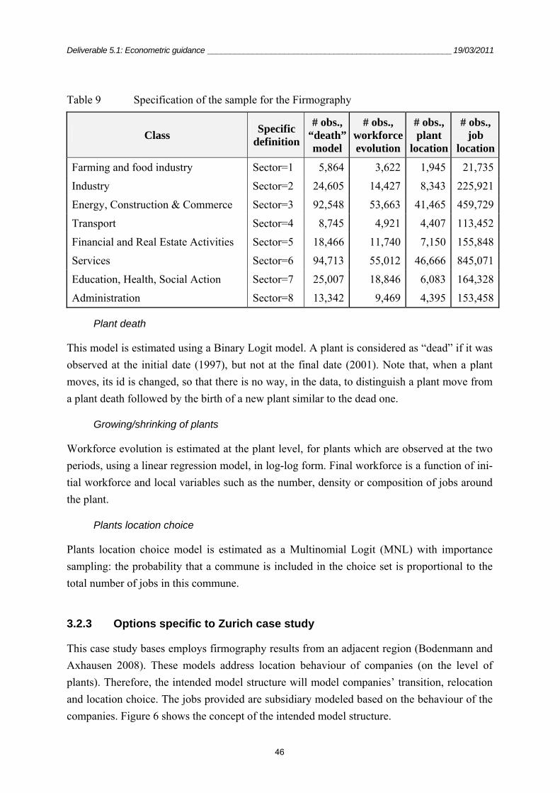
Deliverable 5.1: Econometric guidance ______________________________________________________19/03/2011
46
Table 9 Specification of the sample for the Firmography
Class Specific definition
# obs., “death” model
# obs., workforce evolution
# obs., plant
location
# obs., job
location
Farming and food industry Sector=1 5,864 3,622 1,945 21,735
Industry Sector=2 24,605 14,427 8,343 225,921
Energy, Construction & Commerce Sector=3 92,548 53,663 41,465 459,729
Transport Sector=4 8,745 4,921 4,407 113,452
Financial and Real Estate Activities Sector=5 18,466 11,740 7,150 155,848
Services Sector=6 94,713 55,012 46,666 845,071
Education, Health, Social Action Sector=7 25,007 18,846 6,083 164,328
Administration Sector=8 13,342 9,469 4,395 153,458
Plant death
This model is estimated using a Binary Logit model. A plant is considered as “dead” if it was observed at the initial date (1997), but not at the final date (2001). Note that, when a plant moves, its id is changed, so that there is no way, in the data, to distinguish a plant move from a plant death followed by the birth of a new plant similar to the dead one.
Growing/shrinking of plants
Workforce evolution is estimated at the plant level, for plants which are observed at the two periods, using a linear regression model, in log-log form. Final workforce is a function of ini-tial workforce and local variables such as the number, density or composition of jobs around the plant.
Plants location choice
Plants location choice model is estimated as a Multinomial Logit (MNL) with importance sampling: the probability that a commune is included in the choice set is proportional to the total number of jobs in this commune.
3.2.3 Options specific to Zurich case study
This case study bases employs firmography results from an adjacent region (Bodenmann and Axhausen 2008). These models address location behaviour of companies (on the level of plants). Therefore, the intended model structure will model companies’ transition, relocation and location choice. The jobs provided are subsidiary modeled based on the behaviour of the companies. Figure 6 shows the concept of the intended model structure.

Deliverable 5.1: Econometric guidance ______________________________________________________19/03/2011
47
Figure 6 Intended model structure for Zurich case study
In the Zurich case study, firmography is a three-step model which decomposes the plants and subsidiary jobs evolution:
1. Firmographics events like birth / closures / relocation / growth of plants
2. Location choice of new established plants
3. Location choice of relocating plants
Using data from the three cantons of St.Gallen and both Appenzell, most of these models have been estimated and calibrated. This dataset provides information on more than 50,000 companies during a period from 1991 to 2006. The first model will consist of different sub-models and draw from a macro-econometric transition model.
Due to data restrictions, firmographics in Switzerland generally distinguish between ten sec-tors (Bürgle, 2006; Bodenmann and Axhausen, 2011). The table below gives an overview of the sectors, the number of observed companies during 16 years and the migration rates. If possible, the sector of service and finance is additionally divided in smaller sections: i) fi-nance, ii) business services, and iii) public and personal services (see Bodenmann and Ax-hausen, 2011).

Deliverable 5.1: Econometric guidance ______________________________________________________19/03/2011
48
Table 10 Specification of the sample for the Firmography
Class Specific definition Migrations Migration
rate # of
observations
Service and finance Sector=8 3,168 2.26% 140,468
Wholesale trade Sector=4 1,162 2.22% 52,389
Transport and communication Sector=7 202 1.67% 12,061
Health and educational service Sector=9 145 1.67% 8,672
Manufacturing Sector=2 801 1.35% 59,381
Retail trade Sector=5 574 1.30% 44,293
Construction Sector=3 561 1.22% 45,960
Gastronomy and hotels Sector=6 266 1.14% 23,419
Remaining sectors Sector=10 1 0.88% 114
Agriculture and mining Sector=1 47 0.82% 5,706
All companies 392,463 6927 1.77% 392,463
Firmographic events
In general, this model is based on the results of Bodenmann and Axhausen (2008). Using business demographic data of the cantons of St. Gallen and both Appenzells from the years 1991-2006, four basic variables show up in the migration behaviour of companies: age, size, branch and location (community type) of the business. Using a logit-loglinear model, the relevant effects on the behaviour of the companies have been quantified. A short summary gives the following picture:
• Age: Young companies relocate frequently, especially across longer distances. They also are relatively often affected by business deaths. Newly arrived companies also relocate more often - and they also often change communities at the same time.
• Size: Small companies clearly relocate more often and at further distances than lar-ger ones. Surprisingly, the likelihood that businesses with 10 employees or more will leave their location is no longer dependent on their size.
• Sector: Businesses in growth sectors relocate more often, usually into another com-munity. Businesses dependent on their location basically avoid moving. Especially across larger distances, the likelihood of relocation considerably decreases.
• Location: Clearly more enterprises leave their location in cities than in agricultural areas. A majority of these migrations are between the larger cities.
The results achieved basically confirm the expectations and were also confirmed in various other works. The logit-loglinear model, however, allows showing which effects are brought about by the individual characteristics of the businesses – whereby the effects of all other

Deliverable 5.1: Econometric guidance ______________________________________________________19/03/2011
49
characteristics can be taken into account. For example, several papers point out that young companies relocate frequently. Because young companies are also usually small, the question remains whether company size is responsible for this connection. With the estimated model, this question can be cleared up unambiguously: age and size have an independent effect on the behaviour of a business. The age of a company has a predominant influence on migration behaviour: smaller companies often relocate across community boundaries. In comparison, the size of a business has a noticeable effect on the exit rate: the larger the business, the less likely a closure will occur. The effect on migration rates is therefore considerably smaller.
The present analysis shows that several more factors play a part in the decisions on choice of location: among others, the availability of building land and the price of space. This shows up particularly in the modelled effects between the branches. These themes as well as that of in-frastructure (accessibility for customers and employees) and the behaviour of communities and cantons (i.e., taxes) will be explored in further studies.
Location choice of newly established plants
The location choice model for newly established plants has to be re-estimated with the dataset of St.Gallen region. Based on the results of Bodenmann and Axhausen (2010/2011), Bürgle (2006) and Bodenmann (2006) a Nested Logit (NL) model will be estimated. Generally, the same variables will be used as for the location choice of relocating plants discussed below.
Location choice of relocating plants
In general, this model is based on the results of Bodenmann and Axhausen (2011) using dis-crete choice models. In these models, for each year between 1991 and 2006 the companies face 120 alternatives: all 114 municipalities in the examined perimeter plus 6 municipalities randomly selected out of the rest of Switzerland. The set of alternatives reflects the point of view of the decision making companies: for each observation the first alternative represents the company’s current location. This allows a quasi two-stage hierarchical approach to model the process of decision-making. The first stage determines the probability for each company of moving during the year. The second stage determines the location choice for the moving companies. This hierarchical structure is modelled in a Nested Logit (NL) model with two nests (McFadden, 1978): Nest 1 “Stay” has one alternative (the present location) and nest 2 “Move” contains 119 selectable alternatives.

Deliverable 5.1: Econometric guidance ______________________________________________________19/03/2011
50
Table 11 Ranking of estimated utility parameters for relocating companies
Parameter All** Manufacturing
Whole-sale trade
Retail trade
Gastro hotels
Bus. services
Pers. services
Alternative is a city 1* 3* 2* 1* 1 2 * 1*Cantonal business development 2* 2* 3* 2* 3 3 * 2*Tax burden for joint stock companies 3* 4* 4* 6* 4 4 * 4 Previous site is in a city 4 1* 1 3 2 1 * 8 Municipality with a rail station 5* 6* 5* 4* 5 8 * 3*Index of diversity in sectors of trade 6* 5* 9* 8* 8 5 * 11 Population with graduate degree 7* 8* 14* 7* 6 6 * 14 Motorway connection 8* 10* 6* 10* 11 9 * 6 Tax burden for partnerships 9* 7* 8* 5* 17 7 * 10 Accessibility to employees 10* 9* 10* 9* 12 10 * 5*Share of unbuilt land in building zones 11* 11* 12* 16 14 11 * 9 Process for building licence 12* 15* 11* 12* 9 12 * 13 Employees within the same sector 13* 12* 14 13 9 13 * 18Land price for residential use 14* 13* 13* 18 18 15 * 11Rate of unemployment 15 16 7 11 7 17 6Residual land price for residential use 16* 14* 16* 15 15 16 * 16Residual land price for commerce 17* 17 17 13 13 14 * 15Land price for commerce 18 18 18 16 16 18 16
* Significant parameter according to t-test ** Model including all companies observed, apart from holding companies
Table 11 shows the ranking of estimated parameters in different sectors. They are sorted ac-cording to the relevance of the parameters in a model including companies from all sectors. In general, the most important factors on location decisions of companies are cities, cantonal business development and tax burden. The fact that a potential site is in a city summarizes different advantages and disadvantages of these locations. This result corresponds to the in-novative milieu approach and other agglomeration effects (e.g. Hunecke, 2003; Florida, 2005; Bodenmann and Axhausen, 2010). The differences regarding the valuation of a site in a city suggest that companies in the sector of manufacturing tend to leave cities. In contrast, com-panies in the sectors of retail trade as well as public and personal services significantly tend to choose new locations in cities. The parameters regarding tax burden and cantonal business development indicate the very positive effect of governmental business friendliness. But also the various accessibility indicators play a strong role in most of the models. In general, rail-way stations have a larger impact than motorway connections. Interestingly, the various pa-rameters for land prices have all only minor effects. The strongest effect has land price for residential use, this indicates a crowding-out effect between residential and business use.
Deliverable 5.1: Econometric guidance ______________________________________________________19/03/2011
51
These results show evidence, that governments and politicians have several options to influ-ence the site competition for companies between regions: business friendliness, taxes, and, with a smaller effect, accessibility. Regarding business friendliness, (cantonal) business de-velopment is most visible for companies and therefore has a large impact. However, Deve-reux et al. (2007) showed that grants do not have a strong effect on companies’ decisions. As a consequence, business development is more successful in supporting companies: e.g. during the process of formation or migration, as well as regarding information about potential new sites. All over the world, low taxes are a common instrument to attract companies (and natu-ral persons). The models show, that this is certainly an effective option. Indeed, at least in Switzerland over the last 15 years, taxes in most cantons decreased significantly; so it will be difficult to further lower corporate taxes substantially. In contrast to the first two options for action, accessibility became less important over the last decades (Tschopp, 2007). In this pe-riod, differences regarding accessibility between municipalities and regions became signifi-cantly smaller. Therefore, from a governmental point of view the cost-benefit ratio of such projects lost attractiveness.
3.2.4 Options specific to Brussels case study
Within the model that will be used for the Brussels case study, individual jobs (and not firms) are located. Each type of job has an average surface that consumes when located, thus deter-mining the consumed surface.
The structure of the model is a nested logit with the neighborhood or commune at the higher level and individual building at the lower level. An individual model will be estimated for each job type (yet to be defined from the types of activities defined in the INASTI and other data sources).
The explanatory variables that will be used include:
• Building attributes: surface, price
• Zonal attributes: Demographic variables by zone (aggregated statistics of socio-economics), land use by type, presence of amenities, accessibility measures.

Deliverable 5.1: Econometric guidance ______________________________________________________19/03/2011
52
3.3 Real Estate Price Model
3.3.1 Overview
Real Estate Price Models corresponds to Hedonic price models, including simultaneous re-gressions, which are relevant in the case of imperfect real estate markets.
Two distinctions should be operated in the model: a first distinction between renting and sell-ing, and a second distinction between houses and flats.
The relevance of these distinctions depends on:
• correlations between various prices in the same location
• market shares of each category
• turnover in each category
3.3.2 Options
The Real Estate Price Model (REPM) used the following methods: Simple linear regression, Interval regression, and Spatial correlation (SAR, GWR). These methods can be applied ei-ther on Individual prices or on average local prices.
In UrbanSim, parcel version uses data on individual buildings. In this case, the determinants of real estate prices include both individual and local attributes). Linear regression models are estimated on the log of total selling price, including surface in the regressors list.
Aggregate data are on average prices per m². In this case, only the local attributes will be in-cluded in the regressors list.
Potential determinants of the prices are:
• Individual attributes with building characteristics (surface, age, view)
• Local attributes with accessibility (to jobs, households, activities), neighborhood (households, jobs, land use) and distance to stations.
3.3.3 Options specific to Paris case study
Option 1: Average local prices
The option on average local prices is available both for renters and for buyers. The whole sample available in the Côte Callon is used by the model.

Deliverable 5.1: Econometric guidance ______________________________________________________19/03/2011
53
Estimations are run separately for four segments. The distribution of these segments is un-even over the region, with a higher concentration of flats within Paris, and of single dwelling units (houses) in the outer ring (far away suburbs).
Table 12 Dwelling type and tenure type shares in Paris region, by ring
Number Flat -
Owner Flat -
Tenant House - Owner
House - Tenant
Total Flats
Total Houses
Total Dwellings
Paris 401,126 696,236 7,592 5,958 1,097,362 13,550 1,110,912
Inner Ring 419,138 886,351 56,114 287,114 1,305,489 343,228 1,648,717
Outer Ring 272,951 574,683 134,637 768,469 847,634 903,106 1,750,740
Total 1,093,215 2,157,270 198,343 1,061,541 3,250,485 1,259,884 4,510,369
Percentage
Paris 36.11% 62.67% 0.68% 0.54% 98.78% 1.22% 100.00%
Inner Ring 25.42% 53.76% 3.40% 17.41% 79.18% 20.82% 100.00%
Outer Ring 15.59% 32.83% 7.69% 43.89% 48.42% 51.58% 100.00%
Figure 7 Dwelling type shares in Paris region (irrespectively of tenure type)

Deliverable 5.1: Econometric guidance ______________________________________________________19/03/2011
54
Figure 8 Dwelling type and tenure type shares in Paris region
Figure 7, Figure 8 and Table 12 mainly show a monocentric shape of Paris region, with a high concentration of flats in the center, and a high concentration of houses in the suburbs.
Two minor effects can be seen on the maps: some secondary centers with a higher concentra-tion of flats in major towns in each county in the suburbs, and a small West-East gradient with mode houses on the West than on the East at a given distance from the center.
With only less than 0,9% of the total area, Paris contains more than 24% of flats.

Deliverable 5.1: Econometric guidance ______________________________________________________19/03/2011
55
New segment can be easily added for offices and for retail sector (data was collected for that).
Figure 9 Average dwelling prices by type and tenure in Paris region
Figure 9 presents the distribution of average prices over the region by the category of dwell-ing type and tenure type. Some sets of communes with higher prices can be observed mostly at the west of the region.

Deliverable 5.1: Econometric guidance ______________________________________________________19/03/2011
56
A SURE model (including correlations between residuals of the 4 equations) was also esti-mated. Spatial correlations could be added.
A panel data version can be estimated on more than 10 years available for Cote Callon.
Table 13 Dwelling type and tenure type shares in Paris region, by ring
Class Specific definition # of observations
Rent, flat Variable llocation_indiv 303
Buy, flat Variable lvente_indiv 303
Rent, house Variable llocation_coll 283
Buy, house Variable lvente_coll 283
Option 2: Individual prices
This option is available only for buyers.
Data was collected and partially processed, but models are not estimated yet.
Linear regression on log(selling price), with both individual attributes (including surface) and local amenities attributes included in the list of explanatory variables. Dummy variables for zones and time dummies included in the regression allow to compute a price index specific to zone and time. Panel date and time and spatial correlation techniques can be applied to the zone/time-specific components (dummies and error terms).
3.3.4 Options specific to Zurich case study
Setting up an UrbanSim application for a metropolitan area is a major task and includes, in particular, a significant data collection effort. The task was particularly difficult since there was no tax assessor data or data from commercial sources available for the study area at the required spatial resolution. Eventually, publicly available residential asking rents from a web-based portal were used. The variable selection was found by considering significant explana-tory variables while strictly controlling for multicollinearity.
A detailed study on rent prices in the Canton Zurich has been reported by Löchl for the Greater Zürich Area (Löchl and Axhausen, 2010; Löchl, 2006). This report is based on the same survey of 2005 already mentioned on the location choice of households (see above) but is extended through various variables not included in the default UrbanSim environment. Ex-

Deliverable 5.1: Econometric guidance ______________________________________________________19/03/2011
57
amples will be the sunshine-index of a location, distance of a location to the station or the density of households within 1km.
The list of variables can be categorised in three groups based on the data they are derived from:
1. socio-demographic and functional variables: census of population and enterprises
2. variables derived of the urban context: vector data on networks and point of interests
3. topographic variables: digital height model
These data are available and updated for the current case study and might be integrated in Ur-banSim in future.
For a first run, the model will be kept as simple as possible and will only include data that is demanded by UrbanSim in its default version.
To consider the effect of spatial dependency and spatial heterogeneity, Löchl compared dif-ferent methods of estimation: ordinary least square (OLS), spatial simultaneous autoregres-sive models, geographically weighted regression (GWR). These results might be included in the case study as well.
There are no estimates on purchasing and ownership in the housing sector that could be used at present. The hedonic modelling efforts for the Zürich application of UrbanSim are based on residential rents. For the first run of Zurich the rent prices were scaled to get prices for purchasing. As 93% of the housing-market in Zurich is rental based, this might not be an es-sential issue though.
A special aspect for Zurich will be the kind of ownership for an apartment that is being rented. There are three types of ownership in the canton of Zurich: Private persons, institu-tions and co-operatives. Meanwhile private persons and institutions show a very similar be-haviour aiming for the maximization of their benefit, co-operatives act very differently. They often will rent an apartment for a monthly fee that is about 20-20% below market-prices and will select the person who gets this apartment based on socio-demographic characteristics of this person. Current research at the IVT will thus estimate the behaviour of co-operatives with discrete choice models. A first approach will be MNL-models. eventually those might be ex-tended later.

Deliverable 5.1: Econometric guidance ______________________________________________________19/03/2011
58
Table 14 Ownership of Real Estate (Wuest und Partner, 2010)
Owner City of Zürich Canton of Zürich
Private person 50.00%
Institution 21.00%
Co-operative 18.00%
Beside the residential Real Estate Models also commercial (office) and retail real estate sec-tors should be accounted for. Haase has been concentrating on rent prices within the commer-cial sector in his dissertation (Haase, 2011). He estimates hedonic regression models based on 1010 observations in the canton of Zurich. Those observations represent contracts that were signed in the period of 1994 to 2007. By using random coefficient models Haase also ac-counts for temporal changes, location attributes, building attributes and the form of the con-tract.
No model has been estimated on the real estate prices for the retail sector yet. Ciari and Löchl (Ciari et al., 2008; Löchl, 2008) have been interviewing retail chains. These informa-tion might give a qualitative feedback on the location choice of retailers, as well as the rent-prices being paid. Currently no work is concentrating on this issue though.
Besides real estate prices UrbanSim also demands on landprices. For the project “Zukunft ur-baner Kulturlandschaften” these were derived by scaling the average land prices of a munici-pality according to the spatial distribution found for real estate prices. This will be the ap-proach for the Zurich case study of SustainCity as well.
A core set of variables was used as a starting point to explore the significance of various characteristics of household, dwelling and location. This core set was then tentatively ex-tended by adding further variables. Variables that proved significant comprised mostly loca-tion-related attributes like various densities or travel time to city centre but also characteris-tics of municipalities like the rate of vacant rental units or the tax index and housing unit’s features such as price and size. Interaction terms with socio-demographic attributes of the de-cision-making households were introduced to improve the explanatory power of the models. More detailed results were obtained by estimating separate models for different household types. Those types were formed regarding socio-demographic and socioeconomic features. For choice set selection, random sampling was applied. This approach might later be ex-tended to include stratified sampling strategies making use of similarities between chosen and non-chosen alternatives. For carrying out the sampling procedures a custom made Java pro-gramme was developed.

Deliverable 5.1: Econometric guidance ______________________________________________________19/03/2011
59
Household characteristics are necessary to formulate meaningful variables while other site-related attributes’ influence on location choice does not depend significantly on the type of decision-making household. Significant variables of the final model comprise mostly loca-tion-related attributes like various densities or the travel time to city centre but also character-istics of municipalities like the rate of vacant housing units or the tax index and the housing unit’s features price and size. The structure of the estimated models depends to some degree on data availability issues.
The different structure of the two datasets used for alternative sampling might have precluded variables that could prove significant in a residential location choice model. This assumption will have to be verified by drawing samples from the survey dataset only. Like this, more dwelling-related variables could be tested that are not available in the comparis dataset. Also the differences between the two datasets prevent some location-related variables from being used. On the other hand, using only the survey data greatly reduces the number of alternatives available for sampling.
The revealed preference data does not necessarily reflect the households’ true preferences but also the market conditions. In addition, real world data is often strongly correlated, making it difficult to separate influences of different factors. First experiments with residential location choice models drawing only on survey data have confirmed this proposition by providing less explanatory power.
Stratified sampling making use of similarities between the chosen alternative and the other al-ternatives collated for estimation is one possibility of arriving at more realistic estimations. Behind this strategy stands the concept that a given household will not admit every single housing unit in the region under consideration in its choice set but will probably search for housing in a sub region or among certain types of house. To reflect this heuristic search strat-egy, a selective sampling will be considered.
Variables from the models presented here that cannot be used in a confined model include the distance to place of employment and the size of the housing unit. While households with children can be identified, it might be hard to distinguish those with young children. The young households (age below 35, no children) cannot be safely identified because within the currently envisaged simulation only the age of the respective head of household is known. Therefore a separate confined model will have to be estimated for use within the simulation framework. Future estimation runs will tell what is left of the model’s explanatory power when adjusting it to these constraints. The simulation framework on the other hand opens possibilities to introduce additional information. It utilises a synthetic population of house-

Deliverable 5.1: Econometric guidance ______________________________________________________19/03/2011
60
holds that has been created area-wide for the simulation area (see Bürgle et al. 2005). This makes it possible to calculate e.g. percentages of high-, middle- or low-income households within a certain perimeter, an approximated information that is not publicly available through statistics and has not been used yet for the general model.
3.3.5 Options specific to Brussels case study
The correlation between average Flats and Single-Family Houses (SFH) selling prices, in 2001 (SPF, 2011), was found to be 0.38. Although the correlation coefficient between houses and flats selling prices is statistically significant, it is rather low. This indicates that single-family houses and flats correspond to rather distinct markets in a city like Brussels.
Table 15 gives an overview of the market share of each category of housings.
Table 15 Synthetic list of variables used in the various models of the Paris case study
SustainCity Area Brussels-Capital Region Class
N % N %
Rent, flat 811,358 61.5 111,752 24.4
Buy, flat 405,541 30.7 280,232 61.3
Rent, house 101,381 7.7 65,232 14.3

Deliverable 5.1: Econometric guidance ______________________________________________________19/03/2011
61
Figure 10 Proportion of flats in the total number of housings
Source: Land Registry, 2009
The real estate price model is a hedonic model explaining rents as a function of dwelling and zonal attributes for each unit in each period. In the Belgian Socio-economic Survey (Census 2001) the information on rent prices has been collected through a categorical variable (% lev-els of rent). Therefore, the survey does not give the actual value of the asked rent and the model needs to be estimated using an “interval regression” method. This computational pro-cedure is very similar to the one used in the classical ordered probit model (Wooldridge, 2002). The estimation also considers the implementation of a spatial autoregressive model, where neighboring units share an error component. This method allows dealing with spatial autocorrelation problems, when several observations share unobserved attributes. The model follows Yusuf (2004) and Kim et al. (2003) by considering two spatial units as neighbors when they share common borders.
The data involved in the model estimation are summarized below:
• Dwelling attributes: Size of the unit (surface and number of rooms), building type (house or apartment building)
• Zonal attributes: Demographic variables by zone (aggregated statistics of socio-economics), land use by type, presence of amenities, accessibility measures.

Deliverable 5.1: Econometric guidance ______________________________________________________19/03/2011
62
• Environmental quality attributes (conditional on developing a methodology to update this variables the different periods in the simulation).
3.4 Land Development Model
3.4.1 Overview
This is the less advanced model in the 3 case studies (and in UrbanSim).
3.4.2 Options
UrbanSim basically proposes two options, which are substitutes for the moment. It is desir-able that US can evolve so that these two options are complements, and describe respectively the supply and demand for land, in relation to the politicians or stake holder versus investor points of view.
Stake holder point of view: MOS (MOS=Land Use Type) transition model: choice between the different land use types transition between land use types for a given parcel: MNL with a relatively limited choice set (there are 83 land use types in Paris region, which can be grouped in 9 homogenous aggregated types). Trade-off between competing land uses
Investor point of view: choice between the different locations location choice model for a given project: MNL with importance sampling (trade-off between competing locations for a given project). The list of potential alternatives depends on the land use type attached to the project and on the surface of the project: the project can be located only in parcels (com-munes or IRIS) for which the surface available for this land use type is larger than the surface of the project.
Common initial model: project definition. A project is defined as a parcel which changed detailed land use type. It is characterized by location (parcel ID, geocoded), size, former land user type, and new land use type. This is the upper level of a NL model for either option (=either point of view).

Deliverable 5.1: Econometric guidance ______________________________________________________19/03/2011
63
3.4.3 Options specific to Paris case study
Common initial model: Project definition
A Binary Logit model is estimated for each aggregate initial MOS (9 MOS types). The esti-mation sample is made of all parcels existing at the initial period. A project is born when the parcel changes land use type, based on the most detailed level, MOS in 83 categories. MOS type is observed in 6 years (1982, 1987, 1990, 1994, 1999 and 2003), which defines 5 peri-ods, from 1982-87 to 1999-2003.
Stake holder point of view: MOS transitions for parcels
A project is defined by a change in land use type (MOS) for a given parcel during a given pe-riod; then the project is located in the corresponding parcel. This can be illustrated by the Disneyland Paris project, which is clearly reflected in the data in 1987. It induced the transi-tion of 8.74 km² from land use type 2 (farmland or vacant) into type 3 (recreation area) and 4 (individual dwelling). This project was located over 5 communes in the area “Val d'Europe” covering 29.5 km² in the East of the outer ring of Ile de France. The location of this project in “Val d'Europe” area resulted, between 1982 and 2003, in the following evolution:
• Type 2 (farmland or vacant) fell down from 81% of the area of Val d'Europe in 1982 to 51.4% in 2003;
• Type 3 (recreation area) increased from 1.18% of the area of Val d'Europe in 1982 to 12.3% in 2003;
• Type 4 (individual dwelling) increased from than 6.25% of the area of Val d'Europe in 1982 to 12.74% in 2003.
In the general case, from the stake holder point of view, a project corresponds to a transition from an initial aggregate (9 levels) MOS type to a final aggregate MOS type. The probability of transition depends on
• local population density and structure (e.g. fraction of poor/rich or young/old peo-ple), computed from Census data;
• local employment density and structure (e.g. number or fractions of plants and jobs in each sector), computed from ERE data;
• local land use type (e.g. fraction of land in each aggregate MOS type).
Following de Palma et al (2007) methodology, various definitions of “local” may contem-plated and tested:
• parcels adjacent to the ilôt MOS considered (MOS neighbours),
• IRIS in which the ilôt MOS is located

Deliverable 5.1: Econometric guidance ______________________________________________________19/03/2011
64
• Neighbours of this IRIS
• Commune in which the ilôt MOS is located
• Neighbours of this commune
A Multinomial Logit model is estimated separately for each of the 9 aggregate initial MOS types, which predicts the probability of each of the 9 aggregate final MOS types. Combined with the upper level binary decision to generate a project, it results in a nested logit model.
For this decision, the stake holder compares the returns of various projects, i.e. the competing land use types for a given parcel.
Table 16 Specification of the sample of the LDM
Class Specific Definition # observations
1 Forest Forest and clearing in forest 379,943
2 Farmland or vacant Vacant MOS and Farmland activities 770,352
3 Recreation area Squares and sport infrastructures 235,089
4 Individual dwellings Houses and their garden 789,741
5 Collective dwellings Residential collective 79,062
6 Industrial activities Activities of production 138,071
7 Business activities Market, store and office 18,755
8 Government Building with governmental activities 103,963
9 Transport, under construction Infrastructures of transport and construction 132,319
Investor point of view: project location
From the investor point of view, the decision is to locate a project defined by a surface and a land use type in either parcel which: 1) is large enough to welcome the project and 2) is al-lowed to welcome the project based on restrictions or constraints imposed by the law and/or by the stake holders (e.g. dwellings cannot be built in parcels subject to flood, restrictions are imposed on the density of collective and individual dwellings). This corresponds to a multi-nomial logit model, for which the choice set is specific to each project (based on size and MOS type constraints).
For this decision, the investor compares available locations for a given project, i.e. the com-peting parcels in the choice set for a given project. The determinants of this choice are mainly local amenities (e.g. number of train stations or accessibility to population and to jobs), local population and local employment.

Deliverable 5.1: Econometric guidance ______________________________________________________19/03/2011
65
3.4.4 Options specific to Zurich case study
The initial land use transition model (DPTM, development project transition model)
Data
The initial land use transition model uses two data sources:
1. Dwelling register data of the years 1996 – 2004
2. Zoning plans covering the canton Zurich
By comparing the building stock of sequential years development events are identified. De-velopment events are defined as changes in the land use type. Ten land use types are defined according to the FAR and the shares of residential, retail, industrial and governmental use.
Based on this data a MNL model is estimated to predict the probabilities of transitions. The alternatives are the transitions from the present land use type to a possible other one. The ref-erence is the stay-the-same-option. Explanatory variables are:
1. Number of neighboring cells with equal land use type
2. Distance to next highway exit
3. Travel time to down town Zurich
4. Travel time to Zurich airport
5. Log(Accessibility of population)
6. Log(Accessibility of employment)
7. Vacancy in previous year
In most cases only the number of neighboring cells equal with land use type was significant (Weis, 2006). This is an example of a stake holder point of view model.
The initial development location choice model (DPLCM)
The initial development location choice models are MNL models. They are estimated for 3 industrial types, 2 mixed residential types and 3 strictly residential types. Explanatory vari-ables and parameter estimates can be found in Löchl et al. (2007, 38). This is a site looking for an alternative use type model. This model has been chosen to fulfil the requirements of the UrbanSim gridcell version 4.0 (Löchl and Axhausen, 2008). Notice that development con-straints must be met.

Deliverable 5.1: Econometric guidance ______________________________________________________19/03/2011
66
Developer models
The contemplated developer model tries to model developers as agents inside UrbanSim. This approach tries to consider market characteristics of the supply side that are specific for real estate markets. The issue focused on is heterogeneity or in terms of aggregated terminology segmentation on the supply side (Coiacetto, 2001, 2009, 2007).
Data
The data gathered so far is basically of three types: General descriptives of the Swiss real es-tate markets, records of development projects and snapshots of the building stock. The data sources are described by few words under the following subtitles.
Development projects gathered by Documendia
The entities of the dataset are development projects. These projects have been recorded by Documedia (2010), which is a private company. The purpose for which the data is collected is the information of tradesmen and other potential participants in a real estate development process. The attributes inform about the client for whom the project is built, planer, engineer, location of the construction site, time of construction and the project.
GVZ new buildings
Probably the most reliable dataset describing the building stock in the canton Zurich is ob-tained from the cantonal insurance for buildings (GVZ, 2011). By law each building must have insurance. This data is especially valuable because of its detailed information about uses of buildings and the estimated replacement value. Additional attributes of interest are the building volume and the person id associated with the contractor. Unfortunately, the meta data provided is not very good.
The federal building and dwelling register (GWR)
The federal building and dwelling register is built on the national census 2000 and is run in corporation with the municipalities since 2002. The purpose of the register is to provide basic data on buildings and dwellings in Switzerland for statistical and administrative issues. It is also used as basis for spatial analysis in association with the population and enterprise census. Its conceptual data model is shown in the UML diagram in Figure 11.

Deliverable 5.1: Econometric guidance ______________________________________________________19/03/2011
67
Figure 11: Diagram model of federal building and dwelling register
The census is the organization that gathered the data. The construction project is actually added from the federal building survey, which collects data on construction activities in Swit-zerland. Reported are the projects in need of a license. For buildings this means objects that serve as shelters for humans that have a footprint larger than 2m2 and a height of more than 1m (Kanton Zürich, 1977, §2, 1).
If one obtains snapshots of the building stock for different years, one gets a second source of information for the evolution ob the building stock. For the study area the snapshots exist for each year from 2004 until 2010. The building stock is better recorded with each year which leads to overestimated number of new constructions.
Model options
The first approach will be to estimate MNL models with exogenous supply side market seg-mentation with mutually exclusive subsets. It has to be discussed to how the segmentation on the demand side should be considered. The segmentation is envisaged along the following lines base on the data given:
• purpose (profit oriented, non profit oriented),
• professionalism (professional, occasional) using size, organizational form or fre-quency as proxy
• Strategy type followed (portfolio, object-oriented)

Deliverable 5.1: Econometric guidance ______________________________________________________19/03/2011
68
A second approach is to apply a MNL with continuous interactions which would be applica-ble for investigating influences of professionalism or strategy type. Even though in the latter case the variable is ordinal.
A MMNL model seems to be a promising approach for the segment of single family home builders. For some parameters random distribution would be allowed.
Latent class models will also be estimated, trying to determine the segments endogenously. Different numbers of classes will be tested following the approach of Dong and Gliebe (2010).
The land development model will also face the problem of choice set definition (Lee and Waddell, 2010). Generally, there are the options of stratified, weighted and random choice set sampling, which we will test.
3.4.5 Options specific to Brussels case study
The real estate development model is a two-stage model. The first stage predicts the number of buildings by type to build, estimated as a function of average land prices, expected demand in the future, existing supply, available land and economic indicators like interest rates, un-employment level or annual Gross Domestic Product. The second stage predicts where the buildings will be located; this is achieved using a Logit model where each zone is an alterna-tive. Sampling will be required if a disaggregated zoning is considered (e.g. statistical sec-tors); this will be done following McFadden (1978).
Alternatively, a joint generation-location of supply approach will be tested, based on the max-imization of expected profit of real estate developers.
The explanatory variables that will be considered include:
• Zonal attributes: Demographic variables by zone (aggregated statistics of socio-economics), land use by type, presence of amenities, accessibility measures, average land price
• Environmental quality attributes (conditional on developing a methodology to update this variables the different periods in the simulation)
• Micro and micro economic indicators
Real estate generation model
The Real Estate Generation Model will assume a single representative developer by type of building. The total supply by type will be estimated as a function of average land prices, ex-

Deliverable 5.1: Econometric guidance ______________________________________________________19/03/2011
69
pected demand in the future, existing supply, available land and economic indicators like in-terest rates, unemployment level or annual Gross Domestic Product.
The model will be estimated through a linear regression, using as dependent variable the ob-served amount of new buildings by type in different periods from the SPF Economie (Build-ing permits per period from 1996 to 2008). The explicative variables can be obtained from public sources like the Central Bank or from other databases like the SPF Economie survey.
An alternative model, based on the work of Martinez and Hurtubia (2006), will be tested as an alternative to the simple linear regression econometric model. The aforementioned model considers the generation of new supply to be the outcome of a profit maximization process by a (homogenous) representative real estate developer, where the expected future market prices and the existence of supply or demand surplus have a significant effect in the amount of units to build.
Real estate location choice model
Once the new buildings of each type have been generated for a particular period they are lo-cated by the real estate location choice model.
The location choice model is estimated over observed data on new developments (Building permits per period from 1996 to 2008 and 2009 Land Register). The observed buildings are grouped by type and associated with the attributes of the locations where they were built. A multinomial logit model will be estimated to model the choice of zone.
The main difficulty for the estimation of this model is data preparation. The complete set of attributes that describe a potential location is not available for each possible year. Some at-tributes like average land price are available for several years from the SPF Economie, while other (very relevant) attributes, like the land use by activity, need to be generated from the 2009 Land Register by eliminating registers from a certain year forward. This process will re-quire some assumptions over the distribution of the land use by activity type that will be im-posed over demolished buildings.
Simultaneous supply generation and location model
The assumption of the two-stage supply model is a strong one. The decision of what and how much to build clearly depends on the potential locations for the new supply and the market conditions (level of supply surplus) both at the level of specific zones and the aggregate mar-

Deliverable 5.1: Econometric guidance ______________________________________________________19/03/2011
70
ket. Therefore a model for the simultaneous decision of what, how much and where to build should be more realistic.
Such a model has been originally proposed for the case of non-residential supply (office space) by Farooq et al. (2010). This model is based on expected profit maximization attitude of the builders. The profit’s functional form considers the risk attitude of the developer and the expected utility for different locations. The model has been previously estimated for the city of Toronto. Results showed that this kind of models allow to capture the lagged effects of market conditions on the new supply, by including the current supply (and its distribution) as explicative variables of the producers utility (or profit).

Deliverable 5.1: Econometric guidance ______________________________________________________19/03/2011
71
4 Conclusions and recommendations This section summarizes some of the first lessons that have been obtained from the on-going case studies within the SustainCity project.
4.1 Lessons from case studies
4.1.1 Depending on data availability, find the best econometric strategy for each model
The need for detailed and reliable data has been motivated in this document, along with the difficulties in obtaining and using such data. However, data availability, quality and restric-tions are in general location and application-specific. Therefore, it is not practical to try to de-velop general econometric strategies that would be applicable (let alone effective) in all set-tings. Instead, the modelers should be able to find the “best” econometric strategy for each model, based on the data availability. When detailed data of good quality are not available, a more parsimonious or aggregate model might provide more reliable data than a more detailed and elaborate model (that may not be adequately supported by the data).
4.1.2 Compare estimation results obtained with an econometric software and with UrbanSim until you get exactly the same results
UrbanSim provides facilities for the estimation of econometric models, the results of which can be then used for modeling purposes. It is also possible to estimate models outside of Ur-banSim and then use the estimated coefficients within UrbanSim for simulation purposes. Consistency between the model estimation and simulation is of paramount importance for the credibility of the results. As there are multiple secondary reasons that might obfuscate the model estimation process, it is recommended that UrbanSim model estimation results are compared against standard econometric software (that the modeler is familiar with) to make sure that the data and underlying assumptions made by UrbanSim are indeed understood cor-rectly.
One practical way to verify that the results obtained by the two models are consistent is to use a systematic test “a la Hausman” (Hausman, 1978).

Deliverable 5.1: Econometric guidance ______________________________________________________19/03/2011
72
4.1.3 Endogeneity issue and order for running models
UrbanSim involves the running of a sequence of models in cycle. This type of models is known to suffer from endogeneity, which can have significant implications in the model re-sults. In order to minimize the impact of this problem, it is important to ensure that the model coefficient estimates and the order in which the simulations are run are consistent.
Figure 12: Diagram model of federal building and dwelling register
4.2 “Standardized views”
The objective of this subsection is to provide some practical guidance towards the develop-ment of uniform and “standardized” views. This is particularly important in order to be able to develop some composite insight from the output of the models developed for the various cities (but also among different model forms for the same type of model within applications). The identified suggestions reflect already identified items and it is expected that during the further development of the models further similar suggestions will need to be made to ensure uniformity.
4.2.1 Vocabulary and units
When dealing with buildings/apartments, specific distinction should be made between floor space and land area (cover), in order to avoid confusion. The unit that should be used is

Deliverable 5.1: Econometric guidance ______________________________________________________19/03/2011
73
(square) meters. Floor space indicates the total area of the property (in m2); for example if an apartment is spread in two floors and has 100m2 per floor, then the total floor space should be reported as 200 m2. [The fact that this is a two-story apartment, which could be considered an advantage e.g. for the real-estate price model, could be e.g. captured by an additional explana-tory parameter in the hedonic regression model].
On the other hand, land area (cover) reflects the physical space that a property occupies on the land. For example, a 6-story commercial building with 200 m2/floor would have floor space of 1200 m2 and land area of 200m2.
The unit for monetary measures (e.g. income/cost/rent) should be Euro (€) in all cases, in or-der to provide uniformity and more direct comparisons. When the original data is in another currency (e.g. Swiss Franc, CHF), then they should be converted to Euro.
When values are considered in logarithm, the neperian logarithm should be used, and denoted by ln, in order to avoid confusion.
4.2.2 Results presentation
As it has been presented earlier in this document, UrbanSim applications for different cities within SustainCity involve different types of models, at different granularities. Therefore, it is expected that the results may vary substantially. However, there are some measures that can be taken towards providing coherent results that can be used to perform some meta-analysis. One such aspect that relates to the price levels is the recommendation to use a log-transform (both for the model estimations and presentation of results).
Another price-related aspect that can have a large impact on the reported summary statistics is the way that property prices are used. In particular, using total property prices leads to sum-mary statistics (e.g. R2) with much higher values (than if prices per m2 are used). Therefore, the results will be more easily supported if they are accompanied by these statistics and it is recommended that total property prices are used in the model estimations.
4.2.3 Model outputs for policy assessment
Environmental indicators (environmental disutilities + value of environmental amenities)
The ultimate aim of the research is to provide indicators concerning the sustainability of pol-icy options. Therefore there is a need to focus on the production of meaningful indicators

Deliverable 5.1: Econometric guidance ______________________________________________________19/03/2011
74
based on the outputs of our models. The relevant list of environmental and social indicators is being developed so that it can be produced from the simulations
The variability of the environmental variables is mostly at the grid cell level, which means that, if households are sensitive to environmental variables, the relevant location choice mod-el should be estimated at the grid cell level rather than at the commune level. The average quality of the environment is highly localized (De Palma, 2007). The same research had shown that the negative local amenities are more unequally distributed.
De Palma (2007) examined the diversity of the environmental quality in the Paris housing market and concluded that there is an inequity in the spatial distribution of the amenities in the Paris region such as noise, ‘Zones Urbaines Sensibles’ (areas with high concentrations of social problems) presence of water and forests, of train and subway stations. As a result, the household (re)location choice model should directly be related with environmental variables.
Moons (2008) found that taking into account the travel cost of a visitor of an urban forest to calculate the consumer surplus (which is the difference of the travel cost and the willingness to pay for the visit) and the predicted visits, the recreational value of a base site increases. This means that the travel cost is not negligible and should be included in the model.
The “environmental” indicators that should be included are in the following categories of secondary variables:
• global indicators: greenhouse gas emissions, tropospheric ozone, particles, biodiver-sity
• local indicators: particles, NOx, noise, green areas (not for recreation) and green ar-eas for recreation
The primary variables associated to this are:
• Floor space heated for housing x Type of energy used (electricity, gas, coal, gasoil) + Electricity used x type of generation
• Floor space heated for other purposes than housing+ Type of energy used + Electric-ity used x type of generation
• Industrial energy use x Type of energy used + Electricity used x type of generation
• Type + age of cars, trucks and busses and type of fuel used
• Green areas not for recreation: sufficient to have surface by zone
• Green areas for recreation: quality indicator + travel cost to nearby zone
An example of these concepts through an application of travel costs to urban forests is pre-sented in Moons et al. (2008).

Deliverable 5.1: Econometric guidance ______________________________________________________19/03/2011
75
Value of other amenities
Other amenities, such as the supply of cultural services (e.g. libraries, museums) and other public services (e.g. sport facilities) can be included also as indicators, as they arguably affect the overall utility of the considered areas.
Transport cost indicators
The “transport” variables such as the following local secondary variables: travel time and travel cost for the different types of trips (for each origin) are of interest in this context. These aspects of transport are ultimately the result of
• speed by mode and for peak/off peak
• comfort level (sit or stand) in public transport
• availability of cycling paths and sidewalks
• car ownership.
If one believes in “accessibility” as option value, one needs for every zone of origin, the trav-el time and cost to each type of destination, including:
• rail station or motorway existence (for out-of-zone destinations)
• school (for children)
• job
• grocery store etc.
Housing cost (and quality) indicators
Concerning the “housing cost” in the case of households that rent their home, the variable of interest should be computed as the sum of rent + housing-related cost (maintenance, energy utilities). For inhabitants that own the property the sum of property costs instead of rent paid is needed as the relevant indicator.
For property owners that do not occupy their own property, the model needs the net return of their property.
The quality of a housing unit is clearly related to m³ per person. Furthermore, there are a number of other quality variables that can relate to number of bathrooms, existence of garden, garage or fireplace etc.

Deliverable 5.1: Econometric guidance ______________________________________________________19/03/2011
76
Income variables
Income plays a role in the overall utility experienced by an individual and as such it should be modeled. The following variables can provide a reasonable representation:
• wage income after federal taxes
• property income after federal taxes
• local taxes on income
• local taxes on property values
Value of social interaction
Social interaction can also play an important role in the overall utility. One indicator that could capture this aspect is the homogeneity of population in a zone by education and in-come, information that is available or could be inferred.

Deliverable 5.1: Econometric guidance ______________________________________________________19/03/2011
77
5 Bibliography Abdel-Aty, M. and Abdalla, M. F. (2004). Modeling drivers' diversion from normal routes
under ATIS using generalized estimating equations and binomial probit link function, Transportation, 31(3), 327-348(22).
Abdel-Aty, M., Kitamura R. and Jovanis, P. (1997). Using stated preference data for studying the effect of advanced traffic information on drivers’ route choice, Transportation Research C, 5.
Anselin, L. (1988) Spatial Econometrics: Methods and Models. Dordrecht: Kluwer Academic Publishers.
Anselin, L. (2001) Spatial econometrics. In: Baltagi B. (Ed.) A Companion to Theoretical Econometrics. Oxford : Basil Blackwell, pp. 310 - 330.
Belart, B. (2011) Wohnstandortwahl im Grossraum Zürich, dissertation, ETH Zürich, Zürich.
Ben-Akiva, M. (1973) Stucture of Travel Passenger Demand Models, Ph.D. Dissertation, Department of Civil and Environmental Engineering, Massachusetts Institute of Technology.
Ben-Akiva, M. and J.L. Bowman (1998) “Activity Based Travel Demand Model Systems”, Equilibrium and Advanced Transportation Models, P. Marcotte and S. Nguyen, Eds., Kluwer Academic Publishers.
Ben-Akiva, M. and S. Lerman (1985) Discrete Choice Analysis: Theory and Application to Travel Demand, The MIT Press, Cambridge, MA.
Bierlaire, M. (2003). BIOGEME: A free package for the estimation of discrete choice models ,Proceedings of the 3rd Swiss Transportation Research Conference, Ascona, Switzerland.
BERROIR, S., H. Mathian, T. Saint-Julien, and L. Sanders (2004): "Mobilités Et Polarisations : Vers Des Métropoles Polycentriques," Paris: Programme de Recherche Mobilité et territoires urbains.
Bodenmann, B.R. (2006) Lebenszyklusmodelle für Unternehmen in der Raumplanung, Arbeitsberichte Verkehrs- und Raumplanung, 393, Institut für Verkehrsplanung und Transportsysteme (IVT), ETH Zürich, Zürich.
Bodenmann, B.R. und K.W. Axhausen (2008) Schweizer Unternehmen - quo vaditis? Firmendemographische Trends am Beispiel des Wirtschaftsraums St. Gallen, Raumforschung und Raumordnung, 66 (4) 318-332.
Bodenmann, B.R. und K.W. Axhausen (2010) Synthesis report on the state of the art on firmographics, SustainCity Working Paper, 2.3, IVT, ETH Zürich.
Bodenmann, B.R. und K.W. Axhausen (2011) Location decisions of relocating firms- A discrete choice model for the region of St. Gallen, Switzerland, forthcoming.

Deliverable 5.1: Econometric guidance ______________________________________________________19/03/2011
78
Brasington, D. M., and D. Hite (2005) Demand for environmental quality: a spatial hedonic analysis, Regional Science and Urban Economics 35, 57-82.
Buergle M., Loechl M., Auxhausen K.W (2011) Land Use and Transport Simulation: Applying UrbanSim in the Greater Zurich Area. Institute for Transport Planning Systems (IVT), ETH, Zurich
Bürgle, M. (2006) Modelle der Standortwahl für Arbeitsplätze im Grossraum Zürich zur Verwendung in UrbanSim, Arbeitsberichte Polyprojekt Zukunft urbane Kulturlandschaften, 8, NSL, ETH Zürich, Zürich.
Bürgle, M. (2006) Residential location choice model for the Greater Zurich area, paper presented at 6th Swiss Transport Research Conference, Ascona, 2006.
Chamberlain, G. (1980). Analysis of covariance with qualitative data, Review of Economic Studies, 47, 225-238.
Ciari, F., M. Löchl and K.W. Axhausen (2008) Location decisions of retailers: an agent-based ap-proach, paper presented at 15th International Conference on Recent Advances in Retailing and Services Science, Zagreb, July 2008.
Coiacetto, E. (2001) Diversity in real estate developer behaviour: A case for research, Urban Policy and Research, 19 (1) 43-59.
Coiacetto, E. (2009) Industry Structure in Real Estate Development: Is City Building Competitive?, Urban Policy and Research, 27 (2) 117.
Coiacetto, E. (2007) Residential Sub-market Targeting by Developers in Brisbane, Urban Policy and Research, 25 (2) 257-274.
Debreu, G. (1960) Review of D. Luce Individual Choice Behavior: A Theoretical Analysis, American Economic Review 50, 186-188.
de Palma, A., K. Motamedi, N. Picard, and P. Waddell (2005): "A Model of Residential Location Choice with Endogenous Housing Prices and Traffic for the Paris Region," European Transport, 31, 67-82.
de Palma, A., K. Motamedi, N. Picard, and P. Waddell (2007). Accessibility and Environmental Quality: Inequality in the Paris Housing Market.
Devereux, M.P., R. Griffith and H. Simpson (2007) Firm location decisions, regional grants and agglomeration externalities, Journal of Public Economics, 91 (3-4) 413-435.
Dong, H. and J. Gliebe (2010) Exploring the Taste Heterogeneity in Home Developers’ Location Choice, paper presented at 57th annual north american meetings of the regional science association international, Denver, November 2010.
Farooq, B., Miller, E., Haider, M. (2010) Modelling the Evolution of Office Space Supply. Proceedings of the World Conference on Transport Research (WCTR 2010) July 11-15, 2010.
Florida, R. (2005) Cities and the Creative Class, Routledge, New York.

Deliverable 5.1: Econometric guidance ______________________________________________________19/03/2011
79
Goffette-Nagot, F., I. Reginster, and I. Thomas (2010) Spatial Analysis of Residential Land Prices in Belgium: Accessibility, Linguistic Border, and Environmental Amenities Regional Studies First published on: 17 August 2010 (iFirst).
Greene, W.H. (2000) Econometric Analysis Fourth Edition, Prentice Hall, Upper Saddle River, New Jersey.
Guevara, E. and Ben-Akiva, M. (2005) Endogeneity in residential location choice models, paper presented at TRB meeting.
Haase, R. (2011) Ertragspotenziale – Hedonische Mietpreismodellierungen am Beispiel von Büroimmobilien, dissertation, ETH Zürich, Zürich.
Hausman, J.A. (1978). Specification Tests in Econometrics, Econometrica, 46 (6), 1251–1271.
Heckman, J. (1981). The Incidental Parameters Problem and the Problem of Initial Conditions in Estimating a Discrete Time-Discrete Data Stochastic Process. In Structural Analysis of Discrete Data with Econometric Applications. C. Manski and D. McFadden, editors. MIT Press, Cambridge, MA.
Hsiao, C. (1986). Analysis of Panel Data. Cambridge University Press, Cambridge, U.K.
Hunecke, H. (2003) Produktionsfaktor Wissen: Untersuchung des Zusammenhangs zwischen Wissen und Standort von Unternehmen, Aachener Reihe Mensch und Technik, 45, Wissenschaftsverlag Mainz, Aachen.
Hurtubia, R., Flötteröd, G., and Bierlaire, M. (2010). Estimation techniques for MEV models with sampling of alternatives. Proceedings of the European Transport Conference October 11 - 13, 2010.
Kim, C.W., T.T. Phipps, and L.A. Anselin (2003) Measuring the benefits of air quality improvement: a spatial hedonic approach, Journal of Environmental Economics and Management 45, 24 - 39.
Lee, B.H.Y. and P. Waddell (2010) Residential mobility and location choice: a nested logit model with sampling of alternatives, Transportation, 37 (4) 587-601.
LeSage, J.P. and R.K. Pace (2009) Introduction to spatial econometrics. Boca Raton: Chapman & Hall/CRC.
Löchl, M., M. Bürgle and U. Waldner (2007) Handbuch Simulationsmodell Grossraum Zürich, Arbeitsberichte Polyprojekt "Zukunft urbane Kulturlandschaften", 10, NSL, ETH Zürich, Zürich.
Löchl, M. and K. Axhausen (2008) The Zürich experience, presentation, European UrbanSim Users’ meeting, Zurich, March 2008.
Löchl, M. (2006) Real estate and land price models for UrbanSim’s Greater Zurich application, Arbeitsberichte Polyprojekt Zukunft urbane Kulturlandschaften, 6.

Deliverable 5.1: Econometric guidance ______________________________________________________19/03/2011
80
Löchl, M. (2008) Standortplanung im Detail-/Einzelhandel–Auswertung von Interviews mit Unternehmen in Deutschland und der Schweiz, Arbeitsberichte Verkehrs-und Raumplanung, 492.
Löchl, M. and K.W. Axhausen (2010) Modelling hedonic residential rents for land use and transport simulation while considering spatial effects, Journal of Transport and Land Use, 3 (2) 39–63.
Löchl, (2010). Application of spatial analysis methods for understanding geographic variation of prices, demand and market success.
Louviere, J.J., D.A. Hensher and J.D. Swait (2000) Stated Choice Methods: Analysis and Application, Cambridge University Press.
Luce, R.D. (1959) Individual Choice Behavior, Wiley, New York.
Marissal P., Lokhart Pablo M., Vandermotten C., Van Hamme G., Kesteloot C., « Enquêtes socioéconomiques 2001 – Monographies – Les structures socioéconomiques de l’espace belge, Une exploitation des données d’emploi de l’enquête socioéconomique de 2001 », 2006, SPF Economie, P.M.E., Classes moyennes et Energie, Direction générale Statistique et Information économique
Martínez, F.J., and Hurtubia R. (2006) Dynamic model for the simulation of equilibrium states in the land use market, Networks and Spatial Economics, 6, pp. 55-73.
McFadden, D. (1974) “Conditional Logit Analysis of Qualitative Choice Behavior”, Frontiers of Econometrics, P. Zarembka, Ed., Academic Press.
McFadden, D. (1978) Modelling the choice of residential location, in A. Karlquist, L. Lundqvist, F. Snickars, and J. Weibull (eds.), Spatial Interaction Theory and Residential Location, 75-96, North-Holland, Amsterdam.
McFadden, D. (1981) “Econometric Models for Probabilistic Choice”, Structural Analysis of Discrete Data with Econometric Applications, C. Manski and D. McFadden, Eds., Harvard University Press.
McFadden, D. and Train, K. (2000). Mixed MNL models of discrete response, Journal of Applied Econometrics, 15, 447–470.
Moons, E, Saveyn, B, Proost, Stefan, Hermy, Martin (2008). Optimal location of new forests in a suburban region, Journal of Forest Economics 14(1), p. 5-27.
Ortuzar, J. de. D. and L.G. Willumsen (1994) Modelling Transport, Second Edition, John Wiley and Sons Ltd.
Pholo Bala, A. (2010). Descriptive and Geographical Data for European Cities, SustainCity Working Paper, 2.6, Université Catholique de Louvain, Belgium.
POTTIER, P., and L. SALEMBIER (2007): "Pôles D'emploi Franciliens : Quatre Emplois Sur Dix Dans Les Services À La Production," Paris: INSEE.
Deliverable 5.1: Econometric guidance ______________________________________________________19/03/2011
81
STRATEC (2003), “Evaluation et optimisation des mesures d’accompagnement du RER desservant l’agglomération centrée sur la Région de Bruxelles-Capitale” and FP5 European project SCATTER – “Sprawling cities and transport: from evaluation to recommendations”(2002-2005) – Case study Brussels (STRATEC).
Train, K. (2003). Discrete Choice Methods with Simulation. Cambridge University Press.
Tschopp, M. (2007). Verkehrsinfrastruktur und räunliche Entwicklung in der Schweiz 1950-2000, Dissertation, Universität Zürich, Zürich.
Yusuf, A.A. (2004) Does Air Pollution Affect Property Value? A Hedonic Price Analysis in Jakarta. Mimeo.
Vanneste D., Thomas I., Goossens L. (with the collaboration of De Decker P., Laureys J., Laureyssen I., Querriau X., Vanderstraeten L., Wevers W.), “Enquêtes socioéconomique de 2001 – Monographies - Le logement en Belgique”, 2007, 2007, SPF Economie, P.M.E., Classes moyennes et Energie, Direction générale Statistique et Information économique.
Verordnung über die nähere Umschreibung der Begriffe und Inhalte der baurechtlichen Institute sowie über die Mess- und Berechnungsweisen of 22. June 1977 (Allgemeine Bauverordnung / General Building Regulations).
Waldner, U., M. Löchl, M. Bürgle and K.W. Axhausen (2005) Haushaltsbefragung zur Wohnsituation im Grossraum Z\ürich–Feldbericht, Arbeitsberichte Polyprojekt Zukunft urbane Kulturlandschaften, 1.
Walker, J. L. (2001). Extended Discrete Choice Models: Integrated Framework, Flexible Error Structures, and Latent Variables. Ph.D. Dissertation, Department of Civil and Environmental Engineering, Massachusetts Institute of Technology.
Washington, S. P., Karlaftis, M. G., and F. L. Mannering (2003). Statistical and Econometric Models for Transportation Data Analysis. Chapman & Hall/CRC.
Waddell, P., Borning, A., Noth, M., Freier, N., Becke, M. and Ulfarsson, G. (2003) Microsimulation of Urban Development and Location Choices: Design and Implementation of UrbanSim. Networks and Spatial Economics, 3 (1), 2003, 43-67.
Weis, C. (2006) Schätzung der Wahrscheinlichkeit von Übergängen zwischen Landnutzungstypen im Grossraum Zürich zur Verwendung in UrbanSim, Arbeitsberichte Polyprojekt "Zukunft urbane Kulturlandschaften", 5, Working Paper, NSL, ETH Zurich, Zurich.
Wooldridge, J.M. (2002) Econometrics analysis of cross section and panel data. Cambridge, London: The MIT Press.
Yusuf, A.A. (2004) Does Air Pollution Affect Property Value? A Hedonic Price Analysis in Jakarta. Mimeo.

Deliverable 5.1: Econometric guidance ______________________________________________________19/03/2011
82
Web resources:
General Administration of Patrimonial Documentation (GAPD). Web page: http://fiscus.fgov.be/interfakredfr/Taken/overzicht.htm
DOCUMEDIA (2011). Web page: http://www.docu.ch/
GVZ (2011). Web page: http://www.gvz.ch
SPF Economie, Belgium National Office of Statistics, (2011). Belgium Statistics. Web page: http://statbel.fgov.be/
European Environment Agency (EEA), (2011). Web page: http://www.eea.eu.int/products

Deliverable 5.1: Econometric guidance ______________________________________________________19/03/2011
83
Appendix 1: Data for Paris case study Model
Description Source HLCM Firms ELCM REPM LDM
Age of the HH head RGP1 I
Accessibility: LogSum(generalized transport cost)
Metropolis I
Commune’s Area2 GIS, IAU3 I
% HH with children older than 11 RGP S I I
% HH with children under 3 RGP S I
Accessibility to retail services computed by Poulit method, using private car4
RGP, IAU5 I,S
Distance between the commune centroid and Chatelet (Paris center)
GIS, IAU I I I
Population density RGP S I I I
Distance between the commune centroid and the nearest "Route Nationale"
GIS, IAU I I I I
Distance between the commune centroid and the nearest "Autoroute"
GIS, IAU6 I I
Average travel time, rush hour, public transit7 DREIF8, EGT9 I
Average travel time, rush hour, private car DREIF, EGT I
Employment density (jobs/m²) in 1997 ERE, IAU I,S S
Job accessibility by transit. RGP, IAU I S I,S
Job accessibility by car. RGP, IAU I S I,S I
% foreign born HH heads RGP S I
Log(average office prices) in 1998 Callon I O
Log(average dwelling prices) in 1998 Callon I O
Log of the area (variable CAreaKm2) GIS, IAU I
% HH with a head aged between 35 and 65 RGP S I I
Noise caused by airports10. GIS, IAU I I
% HH with 0 active members RGP S I I I
% HH with 1 active members RGP S I I
% HH with 2 active members RGP S I
% HH with only 1 person RGP S I I
% HH with 2 persons RGP S I I
% HH with more than 2 persons RGP S I

Deliverable 5.1: Econometric guidance ______________________________________________________19/03/2011
84
Model Description Source
HLCM Firms ELCM REPM LDM
% blue collars11 among HH heads, before 199812
RGP13 I,S
% employees14 among HH heads, before 1998 RGP I,S
% white collars15 among HH heads, before 1998
RGP I,S
% HH with a foreign born head, before 1998 RGP I,S I
% HH with 0 worker, before 1998 RGP I,S I
% HH with 1 worker, before 1998 RGP I,S I
% HH with 2 workers, before 1998 RGP I,S I
% HH with only 1 member, before 1998 RGP I,S
% HH with 2 members, before 1998 RGP I,S I
% HH with more than 2 members, before 1998
RGP I,S I
% low-income HH16, before 1998Error: Reference source not found.17
RGP, BDF I,S I
% middle-income HH, before 1998.18 RGP, BDF I,S
% high-income HH, before 1998.19 RGP, BDF I,S I
% HH with a head <35 years old, before 1998 RGP I,S I
% HH with head 35-65 years old, before 1998 RGP I,S
% HH with a head >65 years old, before 1998 RGP S
% area occupied by administrative activities20 MOS I I
% forest area21 MOS I I
% area occupied by retail activities22 MOS I S
% area covered by water23 MOS I I I
Job density in the "pôle d'emploi" in 1997 (jobs/m²).24
ERE, INSEE I,S S
% total commune’s labor force working in the agricultural sector in 1990.
RGP I
% total commune’s labor force working in the agricultural sector in 1999.
RGP I
% total commune’s labor force working in the construction sector in 1990.
RGP I
% total commune’s labor force that is workingin the construction sector in 1999.
RGP I

Deliverable 5.1: Econometric guidance ______________________________________________________19/03/2011
85
Model Description Source
HLCM Firms ELCM REPM LDM
% total commune’s labor force that is working in the industrial sector in 1990.
RGP I
% total commune’s labor force that is working in the industrial sector 1999.
RGP I
% total commune’s labor force that is working in services in 1990.
RGP I
% total commune’s labor force that is working in services in 1999.
RGP I
% commune’s area: medical facilities25 MOS I I
% commune’s area: governmental facilities26 MOS I S
% commune’s area: infrastructures27 MOS I I
% commune’s area: residential land use28 MOS I I S
% commune’s area: industrial land use29 MOS I S
% total HH with low-income30 RGP, BDF S I I
Total population in 1990 RGP I
Total population in 1999 RGP S I I
% commune’s area: Other Activities MOS I S
% commune’s area: green space MOS I I
% commune’s area: residential land use MOS I S
Degree of job specialization, "Pole d'emploi" 31.
ERE, INSEE I,S S
% commune’s area: sport facilities MOS I I
% total HH with high income32. RGP S I I
Degree of specialization of jobs in 1997. ERE I,S S
# subway stations in 1999 GIS, IAU I I I I I
% Farmers among workers RGP I
% Craftsmen, self-employed and head of company among workers
RGP I
% "Cadre" among workers RGP I
% "intermediate workers" among workers RGP I
% employees among workers RGP I
% Blue collar among workers RGP I
% workers with primary education level RGP I

Deliverable 5.1: Econometric guidance ______________________________________________________19/03/2011
86
Model Description Source
HLCM Firms ELCM REPM LDM
% workers with junior high school level RGP I
% workers with complete high school level RGP I
% workers with higher education level RGP I
# railway stations (SNCF and RER) in 1999 GIS, IAU I I I I I
Is in “Ville Nouvelle” Admin. data I I
% HH with a head younger than 35 RGP S I
% HH with a head aged between 35 and 65 RGP S I
% HH with a head older than 65 RGP S
Job density in "Zone d'emploi" (jobs/m²), 1997
ERE, INSEE I,S S
% secondary schools under positive action IAU, MEN I I
% ZFU IAU I
Degree of jobs specialization, "zone d'emploi", 1997.
ERE, INSEE I,S S
% ZUS IAU, admin. data I
Starting date for each îlot observed.33 THEMA I
Ending date for each îlot observed. THEMA I
Population density in 1999 RGP + GIS I,S I
Code of the department Admin. data I I I
1 if commune in department 77 Admin. data I
1 if commune in department 78 Admin. data I
1 if commune in department 92 Admin. data I
1 if commune in department 93 Admin. data I
1 if commune in department 94 Admin. data I
% îlots of type i in year t, commune MOS I,S
Log of the professional tax rate www.impots.gouv.fr I
1 if HH head is of foreign nationality RGP I
Identifier of each îlot MOS I
1 if commune is a part of La Defense borough Admin. data I
Log(professional fiscal base/surface occupied by employment)
www.impots.gouv.fr I
Log of the number of jobs in sector 1 in 1997 ERE34 I,S S

Deliverable 5.1: Econometric guidance ______________________________________________________19/03/2011
87
Model Description Source
HLCM Firms ELCM REPM LDM
Log of the number of jobs in sector 2 in 1997 ERE I,S S
Log of the number of jobs in sector 3 in 1997 ERE I,S S
Log of the number of jobs in sector 4 in 1997 ERE I,S S
Log of the number of jobs in sector 5 in 1997 ERE I,S S
Log of the number of jobs in sector 6 in 1997 ERE I,S S
Log of the number of jobs in sector 7 in 1997 ERE I,S S
Log of the number of jobs in sector 8 in 1997 ERE I,S S
Log of the total number of jobs in 1997 ERE I,S S
Log of income per capita (log(income)-0.5*log(HH size)) in 1999.35
RGP, BDF I
1 if the commune is adjacent to Paris GIS, IAU I
Logarithm of the average arithmetic of the rent of a flat in 1998
Callon I,O
Logarithm of the average arithmetic of the rent of a house in 1998
Callon I,O
Log number jobs of sector 1 in 1997 ERE S I,S
Log number jobs of sector 2 in 1997 ERE S I,S
Log number jobs of sector 3 in 1997 ERE S I,S
Log number jobs of sector 4 in 1997 ERE S I,S
Log number jobs of sector 5 in 1997 ERE S I,S
Log number jobs of sector 6 in 1997 ERE S I,S
Log number jobs of sector 7 in 1997 ERE S I,S
Log number jobs of sector 8 in 1997 ERE S I,S
Logarithm of the average arithmetic of the prizes of a flat in 1998
Callon I,O
Logarithm of the average arithmetic of the prizes of a house in 1998
Callon I,O
Starting MOS type for each îlot observed36 MOS I
Ending MOS type for each îlot observed 37 MOS I,S
# jobs of the “Pole d'Emploi” in sector 1 in 97 ERE, INSEE I,S S
# jobs of the “Pole d'Emploi” in sector 2 in 97 ERE, INSEE I,S S
# jobs of the “Pole d'Emploi” in sector 3 in 97 ERE, INSEE I,S S
# jobs of the “Pole d'Emploi” in sector 4 in 97 ERE, INSEE I,S S

Deliverable 5.1: Econometric guidance ______________________________________________________19/03/2011
88
Model Description Source
HLCM Firms ELCM REPM LDM
# jobs of the “Pole d'Emploi” in sector 5 in 97 ERE, INSEE I,S S
# jobs of the “Pole d'Emploi” in sector 6 in 97 ERE, INSEE I,S S
# jobs of the “Pole d'Emploi” in sector 7 in 97 ERE, INSEE I,S S
# jobs of the “Pole d'Emploi” in sector 8 in 97 ERE, INSEE I,S S
# jobs in sector 1 in 97 ERE I,S S
# jobs in sector 2 in 97 ERE I,S S
# jobs in sector 3 in 97 ERE I,S S
# jobs in sector 4 in 97 ERE I,S S
# jobs in sector 5 in 97 ERE I,S S
# jobs in sector 6 in 97 ERE I,S S
# jobs in sector 7 in 97 ERE I,S S
# jobs in sector 8 in 97 ERE I,S S
# jobs of the “Zone d'Emploi” in sector 1 in 97ERE, INSEE I,S S
# jobs of the “Zone d'Emploi” in sector 2 in 97ERE, INSEE I,S S
# jobs of the “Zone d'Emploi” in sector 3 in 97ERE, INSEE I,S S
# jobs of the “Zone d'Emploi” in sector 4 in 97ERE, INSEE I,S S
# jobs of the “Zone d'Emploi” in sector 5 in 97ERE, INSEE I,S S
# jobs of the “Zone d'Emploi” in sector 6 in 97ERE, INSEE I,S S
# jobs of the “Zone d'Emploi” in sector 7 in 97ERE, INSEE I,S S
# jobs of the “Zone d'Emploi” in sector 8 in 97ERE, INSEE I,S S
# children under 3 RGP I,S
# children under 6 RGP I,S
# children under 11 RGP I,S
# children under 16 RGP I,S
# children under 18 RGP I,S
# workers RGP I,S
size (number of HH members) RGP I,S
# the pseudo-couronne 38. IAU, INSEE I
is in Paris INSEE I I
is in Inner Ring INSEE I
Predicted log of the average rent of a flat 39 THEMA, Callon I O

Deliverable 5.1: Econometric guidance ______________________________________________________19/03/2011
89
Model Description Source
HLCM Firms ELCM REPM LDM
Predicted log of the average rent of a house Error: Reference source not found
THEMA, Callon I O
Predicted log of the average price of a flat Error: Reference source not found
THEMA, Callon I O
Predicted log of the average price of a house Error: Reference source not found
THEMA, Callon I O
1 if the activity sector is 10 in 1997 ERE I
1 if the activity sector is 12 in 1997 ERE I
1 if the activity sector is 13 in 1997 ERE I
1 if the activity sector is 14 in 1997 ERE I
1 if the activity sector is 15 in 1997 ERE I
1 if the activity sector is 16 in 1997 ERE I
1 if the activity sector is 2 in 1997 ERE I
1 if the activity sector is 7 in 1997 ERE I
1 if the activity sector is 8 in 1997 ERE I
1 if the activity sector is 9 in 1997 ERE I
Area of each îlots MOS MOS I
% the total surface of commune’s îlots that are of type i in the year t. 40.
THEMA I,S
Local Tax Pro www.impots.gouv.fr I
Number of employees in the plant in 1997 ERE I,O
1 if 10≤Tot97≤19 ERE I,S
Tot97-10 when 10≤Tot97≤19 ERE I,S
1 if 100≤Tot97 ERE I,S
Tot97-100 when 100≤Tot97 ERE I,S
Logarithm of Tot97 if 100≤Tot97 ERE I,S
1 if Total Workforce in 1997=2 ERE I,S
1 if 20≤Tot97≤49 ERE I,S
Tot97-20 when 20≤Tot97≤49 ERE I,S
1 if Total Workforce in 1997 between 3 and 5 ERE I,S
Tot97-3 when 3≤Tot97≤5 ERE I,S
1 if 50≤Tot97≤99 ERE I,S
Tot97-50 when 50≤Tot97≤99 ERE I,S

Deliverable 5.1: Econometric guidance ______________________________________________________19/03/2011
90
Model Description Source
HLCM Firms ELCM REPM LDM
1 if 6≤Tot97≤9 ERE I,S
Tot97-6 when 6≤Tot97≤9 ERE I,S
Dummy of change of Category of each îlot MOS I
% total population that is young living in the Neighbour communes
MOS, THEMA S I
% total population that is in middle age living in the Neighbour communes
MOS, THEMA S I
% total population that is old living in the Neighbour communes
MOS, THEMA S I
% the total number of neighbor commune’s îlots that are of type i in the year t.
MOS, THEMA I,S
% the total surface of neighbor commune’s îlots that are of type i in the year t.
MOS, THEMA I,S
1 RGP a priori refers to the 1999 census. It will be mentioned in other cases. 2 Computed by GIS 3 Communes’ layer 4 The method proposed by Jean Poulit in 1974, based on the logarithm of product supply at each destination. It takes into account the opportunity (number of employments or shops) at destination j. The utility Sij of a person traveling from origin i to destination j, subtracting travel cost ( Cij ), is:
Sij =λ log �Q j�− Cij ,
where the weighting factor is aαλ = , α is the value of time (VOT), and a is an empirical coefficient
used in the gravity trip distribution model. These parameters have been estimated using travel survey data (EGT).
Accessibility from origin i is the log-sum of the accessibilities over all the destinations, j, given by:
log exp iji j
j
CS Qλ
λ⎛ ⎞⎡ ⎤
= −⎜ ⎟⎢ ⎥⎣ ⎦⎝ ⎠
∑ .
Four Poulit accessibility measures are calculated for two trip purposes (professional and shopping) with two alternative modes (private cars and public transit). 5 Transport model 6 Commune layer and VP network 7 All trips taken are observed 8 Time of transit

Deliverable 5.1: Econometric guidance ______________________________________________________19/03/2011
91
9 Criterion of determination of the rush hour 10 Polls around the zones of airports 11 Workers, codes 1b and 1c for POSP variable in RGP. 12 AEMM not in ('98','99') 13 Variable posp: professional position 14 Employees, codes 1d and 1e for POSP variable in RGP. 15 Engineers and executives, codes 1j and 1k for POSP variable in RGP. 16 Households income are estimated by BDF 17 The level of highest income of the thirty percent poorest population is found.
The percent of population with an income lower than this value is considered for this variable. 18 The level of lowest income of the thirty percent richest population and the level of the highest income of the thirty percent poorest of the population are found.
The percent of population with an income between these two values is considered for these variables. 19 The level of lowest income of the thirty percent richest population is found.
The percent of population with an income higher than this value is considered for this variable. 20 Code MOS 69 21 Code MOS 1 22 Codes MOS 43, 44, 45, 46, 47 and 62 23 Code MOS 9 24 Used variable: EmpAg0 from RGP 25 Codes MOS 58 and 59 26 Codes MOS 48, 61 65, 66, 67 and 69 27 Codes MOS 68 28 Codes MOS 30, 31, 32, 33, 34, 35, 36 and 37 29 Codes MOS 38, 39, 40, 41, 42, 68, 70, 71, 72, 73 and 74 30 Lower tercile regarding per capita income 31 We use a Herfindahl index formulation to measure the degree of specialization on employments in a given geographical unit that can be a commune, an employment pole or an employment zone. The formulation is as below:
In this formulation, s represent the activity sector, ns and N represent the number of employments in activity sector s and the total number of employments. The index value be between 1/S and 1 where the greater values represent more specialized employment structures
For the definition of employement poles, please refer to Berroir et al. 2004 or Pottier et Salembrier 2007. 32 Upper tercile regarding per capita income 33 In the model six dates are observed, so the database included five periods: 1982-1987, 1987-1990, 1990-1994, 1994-1999, 1999-2003. 34 ERE refers to the survey of the year 1997. It will be précises in other cases.

Deliverable 5.1: Econometric guidance ______________________________________________________19/03/2011
92
35 Indicated the category of the îlots MOS observed at the beginning of the period 36 Indicated the category of the îlots MOS observed at the beginning of the period 37 Indicated the category of the îlots MOS observed at the ending of the period 38 1 corresponds in Paris, 2 corresponds at three départements of the Inner Ring, 3 corresponds at seven arrondissements (Argenteuil, Evry, Palaiseau, Saint-Germain-en-Laye, Sarcelles, Torcy, and Versailles) of the Outer Ring and 4 corresponds at height arrondissements (Estampes, Fontainebleau, Mantes-la-Jolie, Meaux, Melun, Pontoise, Provins and Rambouillet) of the Outer Ring 39 Instrumented by professional tax rates and fiscal base 40 Indicates the composition of the communes in term of surface of îlots MOS by type of îlot

Deliverable 5.1: Econometric guidance ______________________________________________________19/03/2011
93
Appendix 2: Data for Zurich case study Model
Description HLCM Firms ELCM REPM LDM
Monthly net asking rent in CHF I O
Monthly net asking rent per square meter in CHF I O
Dwelling's floor area in square meter I I
log residential sqm per person I
Floorspace divided by square root of household size
I
Rent/income – ratio I
Building has a lift I
Dwelling unit has a �replace I
Dwelling unit has one or more balconies I
Dwelling unit has a garden terrace I
Single family house I
House built before 1921 I
House built 1921–1930 I
House built 1931–1980 I
House built 1981–1990 I
House built 1991–2005 I
Percentage of buildings in municipality built before 1971
I I
Rent vacancy rate of municipality I
Vacancy of living units in previous year I
Average travel time to Zürich CBD by car in min I I I
Ln travel time by car to Zurich CBD (Bürkliplatz) I I
Travel time to airport with car I
Log accessibility of population with car I
Log of accessibility to residents I
Log of accessibility to jobs I
Regional car accessibility to employment I

Deliverable 5.1: Econometric guidance ______________________________________________________19/03/2011
94
Model Description
HLCM Firms ELCM REPM LDM
Average distance to social contacts, weighted with number of meetings p.month
I
Exponent of distance to social contacts I
Average distance to place of employment of household members
I
Exponent of distance to place of employment I
Ln accessibility of population with car * dummy car available
I
Ln distance to next highway on-ramp I I
Euclidean distance to next highway exit road I I
Distance to railways < 50m I I
Distance to highway< 100m I I
Autobahn within 100 m I
Regional public transport accessibility to employment
I
Accessibility of population with public transport I
Ln accessibility of population with public transport*dummy car no car
I
Ln distance to next railway station I I
Euclidean distance to next rail station in km I
Daily avg. air noise above 52 dB I
Proximity to major roads or high railway noise level
I
Number of jobs in hotel and restaurant industry within 1 km
I
Density of jobs (jobs in retail trade; per ha in 1km radius)
I
Number of inhabitants in hectare I
Population density (per ha in 1km radius) I
Population density (per ha in 1km radius)*dummy young household
I
Fraction of foreigners in hectare I
Households of same size in radius of 1km I

Deliverable 5.1: Econometric guidance ______________________________________________________19/03/2011
95
Model Description
HLCM Firms ELCM REPM LDM
Density of children (per ha in radius of 500m)*dummy family with young children
I
Number of inhabitants with university degree I
Percentage of persons with university degree in municipality
I
Average per capita income I
Share of households with low income I
Share of households with middle income I
Tax income of municipality per person divided by 1000
I I
Local income tax level for individuals I
Tax index of municipality (ratio of tax rate to cantonal avrg weighted with tax payers multiplied by total tax burden (municipality level)
I
Tax rate for legal persons in the year 2002 I
Slope (percent) I
Slope by 25 m raster I
Visibility of lake surface (>1 km2 ) in hectare I
Ln distance to next lake (>1km²) I
Total visibility of terrain surface in hectare I
Mean sunshine index (mean of nine points of time per year)
I I
Evening solar exposure index I
Density of open space (per ha in radius of 2km) I
constant I I
Distance to primary school I
Number of neighbouring cells with same development type
I
Ln sqm of floor space registered as retail use I
Ln sqm of floor space registered as industrial use I
Ln of sqm of floor space registered as governmental use
I
Unbuilt land as registered in land coverage data I
Number of living units I

Deliverable 5.1: Econometric guidance ______________________________________________________19/03/2011
96
Model Description
HLCM Firms ELCM REPM LDM
Full time jobs equivalents I
Number of jobs in the same sector I
Number of jobs in the service sector I
Number of jobs in the retail sector I
Is the previous site I
Distance to the previous site, lambda of alpha*e^(lambda*distance)
I
Distance to the previous site, alpha of alpha*e^(lambda*distance)
I
Land price for commerce and industry (s) I
Residuals of land price for commerce and industry (s)
I
Land price for residential use (s) I
Residuals of land price for residential use (s) I
Share of unbuilt land in building zones (s) I
Rate of unemployment (s) I
Rate of economically active population with graduate degree (s)
I
Previous site is in a large or intermediate city (d) I
Alternative is a large or intermediate city (d) I
Rate of employees within the same sector (s) I
Index of diversity in different sectors (s) I
Tax burden for partnerships (s) I
Tax burden for joint stock companies (s) I
Municipality with a motorway connection (d) I
Municipality with a rail station (d) I
Accessibility to employees (s) I
Duration of the approval process for building licence application (s)
I
Cantonal business development (s) I


