Econometrica, Vol. 83, No. 6 (November, 2015),...

Econometrica, Vol. 83, No. 6 (November, 2015), 2411–2451

IDENTIFICATION PROPERTIES OF RECENT PRODUCTIONFUNCTION ESTIMATORS

BY DANIEL A. ACKERBERG, KEVIN CAVES, AND GARTH FRAZER1

This paper examines some of the recent literature on the estimation of productionfunctions. We focus on techniques suggested in two recent papers, Olley and Pakes(1996) and Levinsohn and Petrin (2003). While there are some solid and intuitive iden-tification ideas in these papers, we argue that the techniques can suffer from functionaldependence problems. We suggest an alternative approach that is based on the ideasin these papers, but does not suffer from the functional dependence problems and pro-duces consistent estimates under alternative data generating processes for which theoriginal procedures do not.

KEYWORDS: Production functions, productivity, total factor productivity, productiv-ity growth.

1. INTRODUCTION

PRODUCTION FUNCTIONS are a fundamental component of all economics.As such, estimation of production functions has a long history in appliedeconomics, starting in the early 1800s. Unfortunately, this history cannot bedeemed an unqualified success, as many of the econometric problems hamper-ing early estimation are still an issue today.

Production functions relate output to inputs (e.g., capital, labor). Perhapsthe major econometric issue in estimating production functions is the possi-bility that there are determinants of production that are unobserved to theeconometrician but observed by the firm. If this is the case, and if the observedinputs are chosen as a function of these determinants (as will typically be thecase for a profit-maximizing or cost-minimizing firm), then there is an endo-geneity problem and OLS estimates of the coefficients on the observed in-puts will be biased. The literature has devoted much attention to the problemof these biases and approaches to solving them (see, e.g., Marschak and An-drews (1944), Hoch (1955, 1958, 1962), Mundlak (1961, 1963, 1996), Mundlakand Hoch (1965), Christensen, Jorgenson, and Lau (1973), Christensen andGreene (1976), McElroy (1987), Panzar (1989), and Slade (1989)).

Over the past 20 years, techniques proposed by Olley and Pakes (1996)(OP) and Levinsohn and Petrin (2003) (LP) to address this endogeneity prob-lem have seen extensive use in the empirical literature, for example, Pavcnik

1Earlier versions of this paper circulated under the title “Structural Identification of Produc-tion Functions.” Thanks to two co-editors, three referees, and Lanier Benkard, Uli Doraszel-ski, Jeremy Fox, Amit Gandhi, Gautam Gowrisankaran, Jinyong Hahn, Salvador Navarro, ArielPakes, Amil Petrin, Mike Riordan, David Rivers, and seminar participants at UCLA, USC,UCSD, NYU, Columbia, Iowa State, Toronto, ESWC-2005, Yale, Northwestern, Colorado, Indi-ana, Oregon State, Nice, and Stanford for helpful discussions. All errors are our own.

© 2015 The Econometric Society DOI: 10.3982/ECTA13408

http://www.econometricsociety.org/

http://www.econometricsociety.org/

http://dx.doi.org/10.3982/ECTA13408

2412 D. A. ACKERBERG, K. CAVES, AND G. FRAZER

(2002), Criscuolo and Martin (2009), Fernandes (2007), Blalock and Gertler(2004), Alvarez and Lopez (2005), Sivadasan (2009), Ozler and Yilmaz (2009),Topalova and Khandewal (2011), Kasahara and Rodrique (2008), Dollar,Hallward-Dreimeier, and Mengistae (2005), and numerous others (also see thesurvey in Ackerberg, Benkard, Berry, and Pakes (2007)). The essence of the OPand LP techniques is that, under certain theoretical and statistical assumptions,one can invert optimal input decisions to essentially allow an econometricianto “observe” unobserved productivity shocks. More precisely, OP identifiedconditions under which firm-level investment (conditional on capital stock) isa strictly increasing function of a scalar, firm-level, unobserved productivityshock. This strict monotonicity implies that one can invert this investment de-mand function, and thus “control for” the unobserved productivity shock byconditioning on a nonparametric representation of that inverse function (i.e.,a nonparametric function of capital stock and investment). In the first stageof the approach, one estimates the labor coefficient in the production func-tion by regressing output on the labor input and this nonparametric function.LP used a similar approach, but inverted an intermediate input demand func-tion instead of an investment demand function to control for the unobservedproductivity shock.

This paper first argues that there may be a problem with the first stage ofthese estimation procedures. More specifically, under some simple data gen-erating processes that are consistent with the stated assumptions of the OP/LPmodels, the moment condition underlying the first stage estimating equationdoes not identify the labor coefficient. The problem is one of functional de-pendence. Under these data generating processes, one can show that labor isa deterministic function of the set of variables that, in the OP/LP procedures,need to be nonparametrically conditioned on. Hence, once one does this non-parametric conditioning, there is no variation in labor left to identify the laborcoefficient.2 We then explore alternative data generating processes, trying tofind examples where this functional dependence problem does not apply. Wefind only a limited set of data generating processes for which the labor coeffi-cient can be identified using the OP/LP first stage moments, characterize theseprocesses, and argue that they may be unrealistic in many industries.

We then propose an alternative estimation procedure that uses moment con-ditions very similar to those used by OP and LP, but that avoid this functionaldependence problem. Specifically, while OP and LP invert investment (OP)and intermediate input (LP) demand functions that are unconditional on thelabor input, we suggest inverting investment or intermediate demand functionsthat are conditional on the labor input. While use of these conditional input de-mand functions precludes identification of the labor coefficient using the firststage moments, we describe how this coefficient can be estimated along with

2In 1999 Susanto Basu made a less formal argument regarding this possible functional depen-dence problem as a discussant of an earlier version of the Levinsohn–Petrin paper.

PRODUCTION FUNCTION ESTIMATORS 2413

the other production function parameters using the second stage moments (af-ter the first stage moments are used to estimate auxiliary parameters). Wealso illustrate how our use of conditional input demand functions allows forsome more general data generating processes than the original OP and LPprocedures. Unlike the canonical OP and LP moment conditions, our momentconditions produce consistent estimates if there are unobserved, serially cor-related, firm-specific shocks to the price of labor, if labor is chosen prior toother variable inputs (with a different information set), or if labor is dynamicand there are unobserved, firm-specific adjustment costs of labor. Wooldridge(2009) proposed estimating the two sets of moments in LP (or OP) simulta-neously, and argued that doing this avoids the same functional dependenceissue raised in a working paper version of this paper. On the other hand, as wediscuss in Section 4.3.2, the Wooldridge moments as written are based on un-conditional input demand functions and do not allow all the aforementioneddata generating processes.

We start with a quick review of the various approaches that have been used toaddress this endogeneity problem over the past 70 years. We then discuss thepotential functional dependence issues in OP and LP and describe the datagenerating processes necessary to avoid these functional dependence issues.We then present our alternative moments and estimation procedure and dis-cuss in what dimensions these alternative moments extend the data generat-ing processes that can be considered. Lastly, we perform a brief Monte Carlostudy. We consider some data generating processes that are favorable to theLP moments, and some that are favorable to our alternative moments, andas expected, each procedure performs better in the respective data generat-ing process that is favorable to it. Perhaps more interestingly, we then createmisspecification by adding measurement error to the material input variable.Neither our moments nor the LP moments produce consistent estimates, butestimates from our moments are less sensitive than the LP moments to at leastthis form of misspecification.

2. REVIEW OF LITERATURE ON PRODUCTION FUNCTION ESTIMATION

We start with a brief review of the literature on estimation of productionfunctions (borrowing liberally from Griliches and Mairesse (1998)), endingwith a detailed summary of the approaches of Olley and Pakes (1996, hence-forth OP) and Levinsohn and Petrin (2003, henceforth LP). OP and LP are theapproaches which our work most directly assesses and builds on.

For illustration purposes, consider a simple Cobb–Douglas production func-tion in logs

yit = β0 +βkkit +βllit +ωit + εit�(1)

where yit is the log of output, kit is the log of capital input, and lit is the log of la-bor input, all of which are observed. There are two econometric unobservables,


ωit and εit . The εit represent shocks to production or productivity that arenot observable (or predictable) by firms before making their input decisionsat t. In contrast, the ωit represent “productivity” shocks that are potentiallyobserved or predictable by firms when they make input decisions. Intuitively,ωit might represent variables such as the managerial ability of a firm, expecteddown-time due to machine breakdown, expected defect rates in a manufactur-ing process, soil quality, or the expected rainfall at a particular farm’s location.εit might represent deviations from expected breakdown, defect, or rainfallamounts in a given year. εit can also represent (potentially serially correlated)measurement error in the output variable.

The crux of the identification problem inherent in estimating such a produc-tion function is that the inputs kit and lit are chosen by firms. This means thatif the econometric unobservable ωit is observed (or partially observed) by thefirm prior to choosing kit and lit , then these choices will likely depend on ωit ,creating correlation between (kit� lit) and ωit , and rendering OLS estimates ofβk and βl inconsistent. Observation of this endogeneity problem dates back toMarschak and Andrews (1944).

2.1. Prior Approaches

One approach to address this endogeneity problem involved using paneldata with fixed effects, first advocated by Hoch (1955, 1962), Mundlak (1961,1963), and Mundlak and Hoch (1965). The most basic of these approaches in-volves assuming ωit = ωi, where the “fixed effect” ωi is observed by the firmprior to choosing inputs. In essence, the assumption here is that all endogene-ity problems are related to a time-invariant shock ωi. Under this assumption,standard fixed effect approaches can consistently estimate βk and βl. Unfortu-nately, this approach has not worked well in practice; one common finding isunreasonably low estimates of βk and returns to scale. As noted by Grilichesand Mairesse (1998), this could be due to problems with the assumption thatthe only unobservable generating endogeneity problems is time invariant, orit could be due to problems with data (since differencing can exacerbate mea-surement error problems; e.g., Griliches and Hausman (1986)). In recent years,these approaches have been generalized (e.g., Chamberlain (1982), Andersonand Hsiao (1982), Arellano and Bond (1991), Arellano and Bover (1995), andBlundell and Bond (1998, 2000))—see Section 4.3.3.

A second approach has utilized information in firms’ first order conditionswith respect to inputs. Early applications include Klein (1953), Solow (1957),Nerlove (1963), Griliches and Ringstad (1971), and Hall (1988). Generallyspeaking, these approaches consider estimation of first order conditions re-garding, for example, choices of kit and lit . These first order conditions de-pend on input (and output) prices, as well as the production function param-eters (the simplest illustration of this approach is the well-known observationthat in a Cobb–Douglas environment, the first order conditions imply that the


cost shares of each input equal the respective input elasticities). These ap-proaches, including the related idea of estimating cost functions (e.g.. Chris-tensen, Jorgenson, and Lau (1973), Christensen and Greene (1976)), havebeen generalized in a number of dimensions, including some fairly rich the-oretical and statistical models. A good example is McElroy (1987), who uti-lized first order conditions in the context of a production function more gen-eral than (1). McElroy not only considered a more flexible production function(translog), but also a more flexible stochastic specification in which there aremultiple structural unobservables entering in different places in the produc-tion function (instead of only Hicks neutral shocks as in (1)); specifically, thereis one such structural unobservable associated with each of the inputs, so, forexample, some firms are relatively more efficient at using capital, and someare relatively more efficient at using labor. One caveat of these approaches isthat they typically rely on the assumption that input choices satisfy static firstorder conditions. This could be problematic if certain inputs were subject tosignificant dynamic issues, for example, adjustment costs, or wedges betweenpurchase and resale prices. A particular worry with respect to this caveat mightbe the capital input, which in many theoretical models has dynamic implica-tions so that the static first order condition does not hold. In theory, one couldconstruct first order conditions consistent with these dynamic implications, butthese would (1) be considerably more complicated than static first order con-ditions, and (2) likely require additional auxiliary assumptions on the dynamicenvironment firms operate in.

As pointed out by Griliches and Mairesse (1998), a natural extension of theabove “first order condition” approaches involves using input prices as “instru-ments” for the observed inputs in (1), that is, by simply regressing yit on kit

and lit , using pkit and pl

it as instruments. The idea here is that if input pricesare exogenous (i.e., uncorrelated with ωit + εit), and if input choices respondto these input prices (which they should), then these input prices provide asource of exogenous variation in kit and lit with which to identify βk and βl.What is particularly nice about this simple “input price based IV” method isthat its consistency does not require one to specify the relationship betweenthe inputs (kit and lit), and input prices using pk

it and plit correctly. Hence, un-

like the aforementioned work that relies on using static first order conditionsexplicitly, it can produce consistent estimates even if the inputs are dynamic innature (though it will generally not be as efficient if the static first order con-ditions do hold). Of course, these “input price based IV” methods rely on theresearcher observing variation in input prices across firms, and the assumptionthat these input prices are exogenous. Griliches and Mairesse (1998) noteda number of reasons to potentially question this assumption. For it to hold,for example, the observed price differences across firms cannot capture in-put quality differences across firms, or different firms’ choices of location on adownward sloping input supply curve.

Much of the motivation behind the OP (and LP) approaches is related tothe caveats described above. For example, unlike pure fixed effect approaches,


OP and LP do allow for input endogeneity with respect to a time varying unob-servable. Unlike many of the first order condition approaches, they can allowfor subsets of inputs to be dynamic in nature, yet do not require explicit so-lution of complicated dynamic first order conditions related to those inputs.And lastly, unlike the “input price based IV” methods, they do not require theeconometrician to observe exogenous, across-firm variation in input prices.

Of course, relaxing these assumptions does not come without costs. Oneneeds a new set of statistical and theoretical restrictions to produce identifica-tion in the OP and LP models. As detailed extensively below, potentially strongother assumptions need to be made regarding, for example, similarities in theenvironments that different firms face, what variables are in firms’ informationsets when different inputs are chosen, and limiting the amount of unobservedheterogeneity in production functions across firms. We see this paper as con-tributing to the literature by (1) clarifying these statistical and theoretical re-strictions, (2) pointing out some significant caveats of these statistical and the-oretical restrictions related to functional dependence issues, and (3) proposingsome alternative (but very similar) estimators that avoid these functional de-pendence problems. It is important to point out that while we relax a few ofthe assumptions of OP/LP and avoid the functional dependence issue, the keyassumptions behind our approach remain the same. Our approach, like OPand LP, relies critically on timing assumptions, a scalar unobservable assump-tion, and a monotonicity assumption. These potentially strong assumptions arewhat allow for the relaxed assumptions in other dimensions described above.Naturally, whether one chooses our approach or that of the other estimationmethods, one should strive for transparency regarding key assumptions andthen motivate the appropriateness of those assumptions for the relevant em-pirical context.

2.2. Olley/Pakes and Levinsohn/Petrin

Behind the OP and LP identification strategy is a discrete time model of dy-namically optimizing firms. Typically, the primitives of the model are assumedto satisfy the following three assumptions:

ASSUMPTION 1—Information Set: The firm’s information set at t, that is, Iit ,includes current and past productivity shocks {ωiτ}tτ=0 but does not include futureproductivity shocks {ωiτ}∞

τ=t+1. The transitory shocks εit satisfy E[εit | Iit] = 0.

ASSUMPTION 2—First Order Markov: Productivity shocks evolve accordingto the distribution

p(ωit+1 | Iit)= p(ωit+1 |ωit)�

This distribution is known to firms and stochastically increasing in ωit .


ASSUMPTION 3—Timing of Input Choices: Firms accumulate capital accord-ing to

kit = κ(kit−1� iit−1)�

where investment iit−1 is chosen in period t − 1. Labor input lit is non-dynamicand chosen at t.

Assumptions 1 and 2 are straightforward—firms do not observe ωit untiltime t, but the distribution p(ωit+1 | ωit) defines what the firm knows aboutthe distribution of future productivity shocks. Assumption 3 distinguishes thecapital and labor inputs. The labor input is non-dynamic in the sense that afirm’s choice of labor for period t has no impact on the future profits of thefirm. In contrast, capital is assumed to be a dynamic input subject to an in-vestment process. Importantly, Assumption 3 implies that the period-t capitalstock of the firm was actually determined at period t − 1, that is, kit ∈ Iit−1.Intuitively, the restriction behind this assumption is that it takes a full periodfor new capital to be ordered, delivered, and installed. This assumption will beimportant in generating the moment conditions used for estimation. NeitherOP nor LP precisely defined the data generating process (DGP) determininglit . One of the contributions of this paper is to think about this DGP moreformally, which we do in Section 3.

In the above model, firms’ optimal investment decisions iit are policy func-tions resulting from a dynamic optimization problem. Under additional as-sumptions on primitives of the model, OP derived two crucial properties ofthese policy functions. To save space, we simply state these as additional, high-level, assumptions.

ASSUMPTION 4—Scalar Unobservable: Firms’ investment decisions are givenby

iit = ft(kit�ωit)�(2)

ASSUMPTION 5—Strict Monotonicity: ft(kit�ωit) is strictly increasing in ωit .

Assumption 4 states that investment is a function of the state variables kit

and ωit (lit is not a state variable because it is non-dynamic and chosen at t).Griliches and Mairesse (1998) noted that Assumption 4 places strong im-plicit restrictions on additional firm-specific econometric unobservables in themodel. For example, it rules out any unobserved heterogeneity across firms inadjustment costs of capital, in demand or labor market conditions (unless theyevolve independently over time), or additional unobservables entering otherparts of the production function as in McElroy (1987). On the other hand, the


indexing of f by t does allow differences in these variables across time.3 As-sumption 5 is a consequence of the assumptions that p(ωit+1 | ωit) is stochas-tically increasing in ωitand that ωit positively affects the marginal product ofcapital; together, these imply that firms with higher ωit ’s have higher expectedmarginal products of capital in the future, and thus engage in more investment.Formally proving this requires using dynamic programming methods and canbe a challenge in more complicated models. Mechanically speaking, all the re-sults here and in later sections can apply to production functions more generalthan Cobb–Douglas given that Assumptions 1 through 5 hold (so, e.g., theycannot be applied to production functions with multidimensional unobserv-ables like McElroy (1987)).

The econometrician is presumed to observe inputs lit and kit , output yit , andinvestment levels iit for a panel data set of firms with N → ∞ and fixed T .We assume that inputs and outputs are measured in comparable physical unitsacross observations (extensions to this are discussed in Section 4.3.4). Esti-mation in OP proceeds in two stages, each stage corresponding to a distinctmoment condition. To form the “first stage” moment condition, note that As-sumptions 4 and 5 imply that one can invert the investment policy function

ωit = f−1t (kit� iit)(3)

to write the productivity shock as a (unknown) function of observables. Substi-tuting this into the production function, we get

yit = β0 +βkkit +βllit + f−1t (kit� iit)+ εit = βllit +Φt(kit� iit)+ εit �(4)

Because f−1t is the solution to a potentially complicated dynamic programming

problem, deriving its functional form would require additional computationand specifying additional primitives (e.g., the evolution of industry-wide inputprices or demand conditions over time). To avoid this, OP treat f−1

t nonpara-metrically. This clearly precludes identification of β0 and βk using this equa-tion, so these are combined into a composite term Φt(kit� iit) that is treatednonparametrically.

The first stage of OP then generates GMM estimates β̂l and Φ̂t(kit� iit) usingthe moment condition

E[εit | Iit] =E[yit −βllit −Φt(kit� iit) | Iit

]= 0�(5)

3If firm-specific variables such as exogenous labor input prices are observed by the econome-trician, they can be included in (2). However, the premise of most of this literature is that suchvariables are either not available or not believed to be exogenous. If one observed exogenous,across-firm, variation in all input prices, estimating the production function using input pricebased IV methods might be preferred to OP/LP related methodology (due to fewer auxiliary as-sumptions). In other words, OP/LP (and the methods we suggest) are probably most useful whenone does not observe any exogenous across-firm variation in input prices, or when one observesexogenous across-firm variation in input prices for only a subset of the inputs (for the latter, see,e.g., Doraszelski and Jaumandreu (2013)).


If one uses a polynomial approximation to Φt , this can be as simple as runningOLS of yit on lit and the polynomial.

For the “second stage” moment condition, Assumptions 1 and 2 imply thatwe can decompose ωit into its conditional expectation at time t − 1, and aninnovation term, that is,

ωit =E[ωit | Iit−1] + ξit =E[ωit | ωit−1] + ξit = g(ωit−1)+ ξit�

where, by construction, E[ξit | Iit−1] = 0. Substituting this into the productionfunction gives

yit = β0 +βkkit +βllit + g(ωit−1)+ ξit + εit(6)

= β0 +βkkit +βllit(7)

+ g(Φt−1(kit−1� iit−1)−β0 −βkkit−1

)+ ξit + εit�

where the second line follows from the definition of Φt(kit� iit).Given that E[ξit | Iit−1] = 0 and E[εit | Iit] = 0 (which implies that E[εit |

Iit−1] = 0), the second stage of OP’s estimation procedure uses the followingmoment condition:

E[ξit + εit | Iit−1](8)

=E[yit −β0 −βkkit −βllit

− g(Φt−1(kit−1� iit−1)−β0 −βkkit−1

) | Iit−1

]= 0�

where estimation proceeds by “plugging in” the first stage estimates of β̂l andΦ̂t−1 into the second stage moment. Note that the two sets of moments, (5) and(8), that identify the production function parameters and the functions Φt andg can be thought of in the semiparametric moment restriction framework of Aiand Chen (2003) (and as pointed out by Wooldridge (2009), could be thoughtof as IV estimators). While these moment conditions could be estimated jointlyas in Ai and Chen or Wooldridge (2009), estimation using a two-stage “plug-in”approach is consistent (see Ai and Chen (2007)) and popular in the empiricalliterature for computational reasons. Joint estimation requires a numeric, non-linear search over all the parameters of the model (including those represent-ing the functions Φt and g), which can be time-consuming and/or unreliable.The two-stage approach requires at most two sequential smaller dimensionalsearches, and if Φt is specified using polynomials or kernels, the first stage esti-mation of βl and Φt−1 can be done analytically. On the other hand, as pointedout by Wooldridge (2009), there are advantages to estimating the moment con-ditions jointly, for example, potential efficiency gains from information in thecovariances of the moments (though this is not always the case; see Ackerberg,Chen, Hahn, and Liao (2014)), and more straightforward asymptotic standarderrors (see Chen, Hahn, Liao, and Ridder (2013)).


LP take a related approach. The key difference is that instead of using theinvestment demand equation to “invert” out ωit , they use the demand func-tion for an intermediate input mit (e.g., electricity, fuel, or materials). Morespecifically, they consider the following production function:

yit = β0 +βkkit +βllit +βmmit +ωit + εit(9)

and replace Assumptions 4 and 5 with the following:

ASSUMPTION 4B—Scalar Unobservable: Firms’ intermediate input demand isgiven by

mit = ft(kit�ωit)�(10)

ASSUMPTION 5B—Strict Monotonicity: ft(kit�ωit) is strictly increasing in ωit .

Assumptions 4b and 5b again allow one to invert ωit as a function of observ-ables, that is, ωit = f−1

t (kit�mit), analogously to the above. Assumption 4b isconsistent with a model in which lit and mit are non-dynamic inputs that arechosen simultaneously at t, after the firm has observed ωit ; what is crucial isthat ωit is the only unobservable entering the intermediate input demand func-tion. Like in OP, this places restrictions on the underlying model, for example,that firms operate in the same labor and material input markets (or identicallabor and material input markets), and that they operate in the same outputmarket with either homogeneous goods or completely symmetric product dif-ferentiation (or identical output markets). Given these restrictions, Assump-tion 5b is verified by LP under mild assumptions on primitives.

Other than this, LP proceeds identically to OP. The first stage involves usingthe equation

yit = β0 +βkkit +βllit +βmmit + f−1t (kit�mit)+ εit(11)

= βllit +Φt(kit�mit)+ εit(12)

and the moment condition

E[εit | Iit] =E[yit −βllit −Φt(kit�mit) | Iit

]= 0(13)

to obtain estimates β̂l and Φ̂t(kit�mit). These estimates are plugged in to thesecond stage moment condition


=E[yit −β0 −βkkit −βllit −βmmit

− g(Φt−1(kit−1�mit−1)−β0 −βkkit−1 −βmmit−1

) | Iit−1

]= 0


to obtain estimates β̂0, β̂k, and β̂m. LP suggest bootstrapping to obtain stan-dard errors, while Pakes and Olley (1995) provide analytic standard error esti-mators.

2.3. Discussion

As noted by Levinsohn and Petrin, there are a number of advantages to us-ing an intermediate input mit rather than investment iit as a way of “inferring”unobserved productivity. First, theoretically, it can be considerably easier toverify Assumption 5b than Assumption 5; verifying 5 requires analysis of a dy-namic programming problem, but as intermediate inputs are typically assumedto be non-dynamic inputs, verifying 5b does not. Second, in practice, invest-ment data can be lumpy; for example, in firm- or plant-level data sets, one of-ten sees iit = 0. This casts doubt on Assumption 5 (strict monotonicity), at leastfor the observations where iit = 0. While the OP procedure can be adapted towork in this weakly monotonic situation, it requires discarding data with zeroinvestment, which LP noted can sometimes be a significant portion of the data.Moreover, lumpiness might also occur at points other than iit = 0, which ismore problematic.

Another important advantage of LP using an intermediate input is related tothe critique by Griliches and Mairesse (1998). In OP, Assumption 4 rules outany firm-specific unobservables (other than the productivity shock ωit) affect-ing investment demand. This, for example, rules out unobserved capital adjust-ment costs that vary across firms, as well as unobserved, firm-specific shocks toinvestment prices. The LP method does not rule such shocks out—since theintermediate input and labor are non-dynamic inputs that only affect currentprofits, there is no reason for mit to depend on these shocks (conditional onkit and ωit). Of course, LP has an analogous restriction regarding unobserved,firm-specific shocks to the price of intermediate inputs and labor. However,this distinction is not symmetric, since OP also rules out these material or la-bor price shocks (except for the special case where they are independent acrosstime). The reason is that if, for example, unobserved wage shocks are seriallycorrelated, the current wage is related to the marginal revenue product of cap-ital in the future, and thus current investment should depend on the currentwage, violating Assumption 5. So, in summary, neither OP nor LP allow seri-ally correlated, unobserved heterogeneity (across firms) in prices of labor orintermediate inputs, while only OP rules out unobserved heterogeneity (acrossfirms) in the price of investment or capital adjustment costs.

Lastly, note that one can extend these methods to situations where theeconometrician actually observes firm-specific variation in the prices of inputs.If these are assumed exogenous, OP/LP can be applied; the prices can simplybe included in the appropriate input demand functions above and used as in-struments. For example, if exogenous variation in pm

it and plit across firms is ob-

served, these variables should be included in the intermediate input equation,


that is, mit = ft(kit�ωit�pmit �p

lit), and included in the instrument set Iit . That

said, both OP and LP make many auxiliary assumptions, so if one observed ex-ogenous, firm-specific variation in all input prices, it might be preferable to usesimple “input price based IV” methods, that is, regress yit on kit , lit , and mit

using pkit , p

lit , and pm

it as instruments. This would provide consistent estimateswithout the OP/LP auxiliary assumptions. Of course, the observed price differ-ences across firms need to be exogenous, that is, the differences cannot captureinput quality differences or different firms’ choices of location on a downwardsloping input supply curve. Having credibly exogenous, observed, variation inthe costs of all inputs is fairly rare. Perhaps more likely is a case where one ob-serves exogenous variation in prices of a subset of the instruments. In this case,pure “input price based IV” methods are generally not possible, and we feelthat techniques related to OP/LP are valuable. Doraszelski and Jaumandreu(2013) estimated a model where this is the case.4

3. FUNCTIONAL DEPENDENCE PROBLEMS

This paper argues that even if the above assumptions hold, there are iden-tification problems with these methodologies. The issue is one of functionaldependence in the first step of the respective procedures. We illustrate theseissues in the LP context, though one can make very similar arguments in theOP context. To give a brief intuition behind the result, consider a parametricversion of the first stage of LP where instead of treating (10) (and its inverse)nonparametrically, one actually uses the parametric FOC corresponding to aCobb–Douglas production function. The first order condition for mit (condi-tional on kit , lit , and ωit) is

βmKβkit L

βlit M

βm−1it eωit = pm

py

�

assuming firms are price takers in both input and output markets.5 Invertingthis equation for ωit and substituting into the production function results in

yit = ln(

1βm

)+ ln

(pm

py

)+mit + εit �(15)

4In contrast to OP and LP, they treat the inverted input demand function parametrically. Theyhave two good reasons for this. First, including observed input prices in the inverted function in-creases the dimensionality of the function and makes nonparametric treatment more challenging.Second, since the production function has already been modeled parametrically, one can obtainparametric forms of input demand functions for non-dynamic inputs without significant auxiliaryassumptions. Doraszelski and Jaumandreu also extend the OP/LP model to one in which ob-served firm R&D expenditures affect the evolution of ωit , an important idea that could also beapplied in the context of our estimation procedure.

5This version of the first order condition assumes that εit is pure measurement error in yit(if εit was an unanticipated shock to output, the expectation of exp(εit) would enter the firstorder condition as well).


Since βl does not enter this expression, a moment condition in εit based on thisequation (which is analogous to the first stage of LP) cannot be informativeon βl.6

While the above result might not hold for more general functional forms ofthe production function, the LP and OP procedures treat the inverted FOCsnonparametrically, which makes identification tougher. The first step momentcondition (13) used to estimate βl in LP is equivalent to the partially lin-ear model studied by Robinson (1988). His condition for identification of βl

(Equation 3.5; see also Ai and Chen (2003), Assumption 3.3 and discussion) isthat

E[{lit −E[lit | kit�mit� t]

}{lit −E[lit | kit�mit� t]

}′]is positive definite�(16)

An immediate observation is that if lit is functionally dependent on kit , mit ,and t (i.e., lit is only a function of kit , mit , and t), this condition does not hold.Intuitively, the problem here is that lit is fully determined by the values ofkit , mit , and t, so there is no source of variation in lit (conditional on kit , mit ,and t) to identify βl. So we focus our discussion on investigating possible datagenerating processes for lit and ask the question whether these DGPs generatethis functional dependence.

Perhaps the simplest possible DGP for lit is analogous to that for mit (equa-tion (10)), that is,

lit = ht(kit�ωit)�(17)

This assumes that, like mit , labor has no dynamic implications and is chosenwith full knowledge of ωit . With this DGP, substituting the inverted (10) into(17) results in

lit = gt

(kit� f

−1t (kit�mit)

)�

which states that lit is functionally dependent on kit , mit , and t, and implies thatthe identification condition (16) fails. Intuitively, in equation (12), the contri-bution of labor to output cannot be separately identified from the nonpara-metric function Φt(kit�mit).

That said, while (17) might be the simplest specification for the data gener-ation process for lit , it is not the only possibility. Our goal now is to search foran alternative DGP for lit (and possibly for mit) that does not suffer this func-tional dependence problem and is consistent with the basic assumptions of theLP (and OP) procedure(s).

6The above analysis uses the choice of mit conditional on levels of kit , lit , and ωit . This is mostnaturally interpreted in the case where mit is chosen after lit . One obtains the same result if onesolves simultaneously for optimal choices of both mit and lit conditional on levels of kit and ωit ,and plugs the inverted FOC for mit into the production function.


First, consider adding firm-specific input prices to the above model of inputchoice, for example, prices of labor (pl

it) and materials (pmit ). Generally speak-

ing, both of these firm-specific input prices will affect a firm’s choices of both litand mit (i.e., conditional on pm

it , decreasing plit will generally increase a firm’s

optimal level of both lit and mit). Therefore, these input prices would need tobe observed by the econometrician, because otherwise (10) would violate thescalar unobservable assumption necessary for the LP inversion. Since interme-diate input demand depends on these firm-specific input prices, they end up inthe first step nonparametric function, that is,

E[εit | Iit] =E[yit −βllit −Φt

(kit�mit�p

lit�p

mit

) | Iit]= 0�(18)

and there is again a functional dependence problem, as there are no variablesthat shift lit but do not enter Φt . Another possibility, allowing labor to havedynamic effects, does not help for the same reason. lit−1 becomes a state vari-able of the problem, but since both mit and lit both depend on lit−1, there is stillfunctional dependence.

One way to eliminate the functional dependence problem is to assume thatthere is “optimization error” in lit . By optimization error, we mean that thereis an optimal level of lit (e.g., given by (17)), but that for some reason the firmchooses that optimal level plus noise (that is independent over time and ofother errors in the model). One example of this could be workers calling insick.7 Such optimization error induces variation in lit conditional on kit , mit ,and t, and hence the first step can consistently estimate βl. However, note thatthe methodology is not compatible with similar optimization error in mit , sincethis would violate the scalar unobservable assumption required to invert (10)and obtain ωit . The context of sick days is a good way to illustrate this pointwith some applied relevance. Suppose that mit are material inputs used in pro-duction and that when workers are out sick, less of these materials are used.If the econometrician’s measure of mit is the actual level of material inputused (which is negatively affected by sick days), there is implicitly optimiza-tion error in both lit and mit , and because of this optimization error in mit , thefirst step will not produce consistent estimates of βl. However, if the econo-metrician’s measure of mit is the planned level of material input used (i.e.,planned/ordered prior to the realization of sick days, and thus unaffected bysick days), there is only optimization error in lit and the first step will produceconsistent estimates of βl. In contrast, the i.i.d. “optimization error” in lit DGPmight not be a good representation of a situation where firms’ labor choices aredistorted by exogenous union issues. This is because union issues are unlikely

7Note the difference between our “optimization error” and the “optimization error” describedby Mundlak (1996). We are simply adding exogenous noise to the desired input level (workersexogenously calling in sick). Mundlak described “optimization error” due to incomplete informa-tion; for example, firms choose labor input based on an expected price of labor, but the realizedprice of labor is different, making their choice of labor input seem suboptimal ex post.


to be i.i.d. over time, and hence either planned or used material inputs arelikely to respond to the (unobserved) union shocks, violating the scalar unob-servable assumption. Note that classical measurement error in lit (i.e., noisein observed labor that does not affect output) is problematic because of stan-dard measurement error problems, and classical measurement error in mit isproblematic because it again violates the scalar unobservable assumption thatis crucial for the inversion.

A second, similar, DGP that can eliminate the functional dependence prob-lem involves changing the assumption that lit and mit are chosen with the sameinformation set. Consider a point in time, t−b, sometime between period t−1and t (i.e., 0 < b< 1).8 First, note that if one assumes lit is chosen at t − b andmit is chosen at t, there is a problem because in such a model, optimal mit willgenerally directly depend on the previously chosen level of lit . Since lit enters(10), the first step moment becomes

E[εit | Iit] = E[yit −βllit −Φt(kit� lit�mit) | Iit

]= 0�(19)

which obviously precludes identification of βl in the first step. However, onecan alternatively consider the reverse situation, that is, where mit is chosen att − b and lit is chosen at t. Suppose there is some unanticipated firm-specificshock to the price of labor (or demand), κit , that is realized between the pointst − b and t (i.e., it is not in the firm’s information set (Iit−b) when mit is cho-sen, but it is in the firm’s information set (Iit) when lit is chosen). Such a shockwill vary lit independently of kit , mit , and t, and thus will eliminate the func-tional dependence problem. This shock κit does not need to be observed bythe econometrician, but if it is unobserved, it must be i.i.d. over time (other-wise the optimal mit+1 will depend on κit , violating the scalar unobservableassumption). Another assumption that is required in this DGP is that the firmobserves ωit when choosing mit at time t − b (perhaps more intuitively, thatω does not evolve between time t − b and time t). Otherwise, the nonpara-metric function of mit and kit will not perfectly control for ωit in the momentcondition.

These functional dependence problems (and possible assumptions thatavoid them) generalize to the first step of the OP procedure that alternativelyuses the investment function to control for productivity variation. Firm-specificinput prices (observed or unobserved) and dynamics in lit generally do notbreak the functional dependence, but optimization error in lit or i.i.d., firm-specific wage (or output price) shocks after iit is chosen do. There is one addi-tional DGP that breaks the functional dependence problem in the OP setup.

8Note that we continue to assume that production occurs “on the period,” that is, at periodst−1 and t. Note that this intermediate period, t−b, does not need to have a literal interpretationin terms of time. What we are simply trying to do is allow different inputs to be chosen withdifferent information sets, and with this heuristic device, an “input chosen at t” is chosen withmore information than is an “input chosen at t − b,” which is chosen with more information thanis an “input chosen at t − 1.”


Continuing with the above setup with the “subperiod” t − b, assume that ωevolves between t − 1, t − b, and t according to a first order Markov process,that is,

p(ωit−b | Iit−1)= p(ωit−b | ωit−1)(20)

and

p(ωit | Iit−b)= p(ωit |ωit−b)�(21)

Suppose also that lit is chosen at time t − b with information set Iit−b, while iitis chosen at time t with information set Iit .

In this case, a firm’s optimal investment will follow

iit = ft(kit�ωit)�(22)

while a firm’s optimal labor input will not be a function of ωit , but of ωit−b, thatis,

lit = gt(ωit−b�kit)�

Since ωit−b cannot generally be written as a function of kit and iit , lit will notgenerally be functionally dependent on kit and iit , possibly allowing consistentestimation of βl in the first step. Note the intution behind this—labor is chosenwithout perfect information about what ωit is, and this incomplete informationis what generates variation in lit conditional on the nonparametric functionf−1t (kit� iit). However, note that this DGP does need to rule out a firm’s choice

of lit having dynamic implications. If labor did have dynamic effects, then litwould directly impact a firm’s choice of iit . As a result, lit would directly enterthe first stage nonparametric function and prevent identification of βl in thatfirst stage.9

3.1. Discussion

To summarize, it appears that the first stage of the OP and LP procedurescorrectly identifies βl only under three very specific DGPs: (1) i.i.d. optimiza-tion error in lit (and not in mit (or iit)); (2) i.i.d. shocks to the price of labor oroutput after mit (or iit) is chosen but prior to lit being chosen; or (3) (in the OPcontext) labor is non-dynamic and chosen at t − b as a function of ωit−b, while

9Note why this DGP does not solve the functional dependence problem in the context of theLP model. In the LP model, if lit is chosen before mit , then mit will directly depend on lit , makingβl unidentified in the first stage. In OP, even if lit is chosen before iit , iit does not depend on lit(as long as one maintains the assumption that labor is non-dynamic). This is because iit , unlikemit , is not directly linked to period-t outcomes, and thus lit will not affect a firm’s optimal choiceof iit .


iit is chosen at t. Note that in practice, one probably would not literally observethe functional dependence problem described above (if one were using poly-nomials to approximate the nonparametric function, functional dependencewould arise in the form of collinearity between lit and the terms in the polyno-mial approximation). In other words, it is likely that estimation of (5) or (13)will produce an actual numerical estimate of βl. Our point is that unless onebelieves that one of these three DGPs is generating the data (and additionallythat these DGPs are the only reasons why there is no functional dependence),this is simply not a consistent estimator of βl.

4. OUR ALTERNATIVE PROCEDURE

We now propose an alternative estimation procedure that avoids the func-tional dependence problems discussed above. Perhaps just as importantly, italso relaxes other assumptions typically made in applications of OP and LP.Specifically, our model allows there to be exogenous, serially correlated, un-observed firm-specific shocks to the price of labor, or firm-specific unobservedadjustment costs to the labor input. It also allows the labor input to have dy-namic effects (e.g., hiring or firing costs) more generally. We emphasize thatthe approach is only a slight adaptation of the OP/LP methodologies, and es-sentially relies on the same moment conditions. The main difference betweenour approach and OP and LP is that in our approach, we invert “conditional”rather than “unconditional” input demand functions to control for unobservedproductivity. This results in a first stage that does not identify the coefficientson variable inputs (e.g., labor). Instead, all coefficients are estimated in thesecond stage. However, as we shall see, the first stage will still be important to“net out” the untransmitted error εit from the production function. We startby showing how our method works using the LP intermediate input functionbefore showing the extension to using the OP investment function.

4.1. The Basic Procedure

Consider the “value-added” production function

yit = β0 +βkkit +βllit +ωit + εit(23)

with the following alternative assumptions:

ASSUMPTION 3C—Timing of Input Choices: Firms accumulate capital ac-cording to

kit = κ(kit−1� iit−1)�

where investment iit−1 is chosen in period t − 1. Labor input lit has potential dy-namic implications and is chosen at period t, period t − 1, or period t − b (with0 < b< 1).


ASSUMPTION 4C—Scalar Unobservable: Firms’ intermediate input demand isgiven by

mit = f̃t(kit� lit�ωit)�(24)

ASSUMPTION 5C—Strict Monotonicity: f̃t(kit� lit�ωit) is strictly increasingin ωit .

First, note that we consider a “value-added” production function in the sensethat the intermediate input mit does not enter the production function to be es-timated. One interpretation of this is that the gross output production functionis Leontief in the intermediate input, where this intermediate input is propor-tional to output (e.g., see our Monte Carlo specification, or Gandhi, Navarro,and Rivers (2014)). Another follows the existing literature on value-added pro-duction functions; see, for example, Bruno (1978) and Diewert (1978). As dis-cussed in those papers, as well as in Basu and Fernald (1997), the assump-tions behind the existence of a meaningful value-added production functionare subtle and nontrivial. We would not suggest applying our procedure togross output production functions that are not Leontief in the intermediate in-put(s) (i.e., production functions where mit enters (23)). This is because Bondand Söderbom (2005) (for the Cobb–Douglas case) and Gandhi, Navarro, andRivers (2014) (for the general case) have shown that under the scalar unobserv-able assumptions of OP, LP, and our procedure, these gross output productionfunctions are not identified without imposing further restrictions of the model.If one is interested in doing this, it is likely preferable to use an approach whereOP/LP-like moments are augmented by first order conditions or revenue shareequations, for example, LP (Appendix B) and Doraszelski and Jaumandreu(2013), who did this in the context of a Cobb–Douglas production function,or Gandhi, Navarro, and Rivers (2014), who show how to do this much moregenerally.

Moving to the assumptions of the model, Assumption 3c generalizes As-sumption 3 by allowing labor to have dynamic implications, that is, choice of litnot only affects current profits, but future profits, for example, through hiringor firing costs. Note that this implies that lit is part of the state space of thefirm’s dynamic problem. We can allow lit to be chosen at period t (and thus afunction of Iit), chosen at period t − 1 (and thus a function of only Iit−1), or atsome point in between (with an intermediate information set).

Assumption 4c represents the crucial conceptual difference between ourprocedure and LP. The difference between Assumption 4b and Assumption 4cis that we are using a conditional input demand function to control for unob-served productivity, while LP uses an unconditional (or less conditional) inputdemand function. More precisely, (24) is the input demand function for mit

conditional on lit , while (10) is the input demand function for mit not condi-tional on lit . While our conditional input demand function might be most nat-urally thought of as representing a situation where mit is chosen after lit , it can


equally well represent a situation where mit and lit are chosen simultaneously.10

As does Assumptions 4 and 4b, Assumption 4c rules out production functionswith multiple structural unobservables like McElroy (1987). Assumption 5c isthe strict monotonicity assumption necessary for the inversion; since mit is stilla non-dynamic input, it is straightforward to apply the invertibility proof of LPto obtain this result.

Given these assumptions, we can follow LP, invert intermediate input de-mand ωit = f̃−1

t (kit� lit�mit), and substitute into the production function, thatis,

yit = β0 +βkkit +βllit + f̃−1t (kit� lit�mit)+ εit = Φ̃t(kit� lit�mit)+ εit �(25)

Since we follow LP and treat f̃−1t nonparametrically, the first three terms are

clearly not identified and are subsumed into Φ̃t(kit� lit�mit) = β0 + βkkit +βllit +ωit , resulting in the following first stage moment condition:

E[εit | Iit] = E[yit − Φ̃t(kit� lit�mit) | Iit

]= 0�(26)

Unlike LP, (26) does not permit estimation of βl in the first stage. However,it does produce an estimate ̂̃Φt(kit� lit�mit) of Φ̃t(kit� lit�mit). We propose esti-mating βl along with the other production function parameters in the secondstage using the following second stage conditional moment:


=E[yit −β0 −βkkit −βllit

− g(Φ̃t−1(kit−1� lit−1�mit−1)−β0 −βkkit−1 −βllit−1

) | Iit−1

]= 0�

where Φ̃t−1 is replaced by its estimate from the first stage. Note that this mo-ment condition is essentially identical to that used by LP (i.e., equation (14)),except for the fact that since Φ̃t−1 now contains the labor term, it also needs tobe subtracted out inside the g function.

As usual, it is easiest to transform conditional moments into unconditionalmoments for actual estimation. It is important to note that since our secondstage requires estimating an additional parameter (βl) as compared to LP, werequire an additional unconditional moment relative to LP. To illustrate, con-sider a simple model where ωit = ρωit−1 + ξit . Suppose the first stage is per-formed by OLS regression of yit on a high-order polynomial in (kit� lit�mit) toobtain ̂̃Φt(kit� lit�mit). If labor is assumed to be chosen after time t − 1 (imply-

10There is no loss of generality in representing maxlit �mit{·} as maxlit {maxmit |lit {·}}. Note that

LP’s unconditional (on lit) intermediate input demand equation, that is, mit = ft(kit �ωit), is mostnaturally interpreted as a situation where lit and mit are chosen simultaneously as a function ofthe current state (kit �ωit).


ing lit will generally be correlated with ξit), a natural set of four second stagemoment conditions to estimate the three production function parameters (β0,βk, and βl) and ρ is

E

⎡⎢⎣(yit −β0 −βkkit −βllit(28)

− ρ · (Φ̃t−1(kit−1� lit−1�mit−1)−β0 −βkkit−1 −βllit−1

))⊗⎛⎜⎝ 1

kit

lit−1

Φ̃t−1(kit−1� lit−1�mit−1)

⎞⎟⎠⎤⎥⎦

= 0�

In contrast, second stage LP estimation based on (14) only requires three mo-ments, though as exemplified in the LP empirical work, one could alternativelyutilize all four moments (or more than four using other components of Iit−1)and have overidentifying restrictions.11

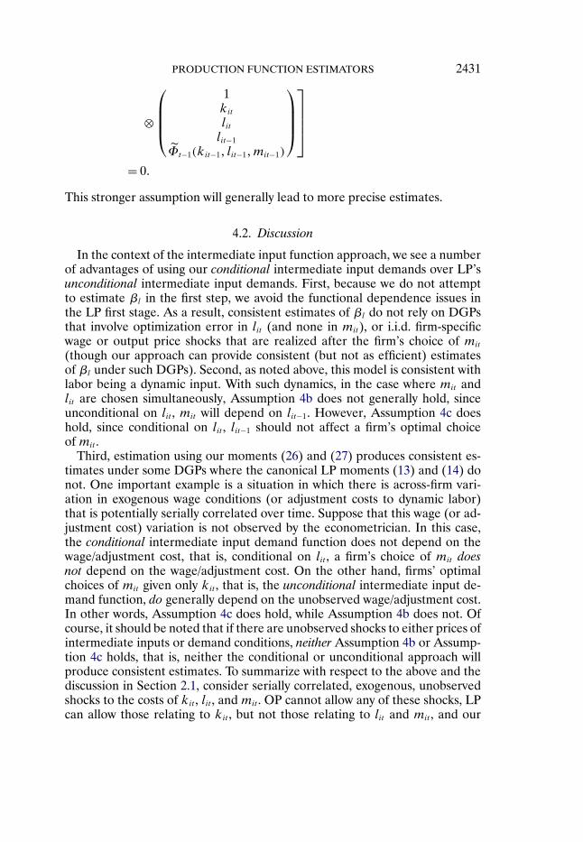
In some industries, one might be willing to assume that labor is chosen by thefirm at t − 1, that is, lit ∈ Iit−1 (or alternatively make the assumption that ωit isnot observed by the firm until period t+1). This is a potentially strong assump-tion, but it might be plausible in situations where there are significant hiring orfiring costs, or labor market rigidities, possibly due to government regulation.In this case, one could add lit to the information set (or replace lit−1 with lit inthe instrument set if one wanted to keep the model exactly identified), that is,

E

⎡⎢⎢⎢⎣(yit −β0 −βkkit −βllit(29)

− ρ · (Φ̃t−1(kit−1� lit−1�mit−1)−β0 −βkkit−1 −βllit−1

))11There are many ways to estimate the model based on the second stage moments. For exam-

ple, the Appendix in LP illustrates how one can do second step estimation with a nonlinear searchover just (βk�βl). A similar approach can work here, where one only has to search over (βk�βl)rather than over (β0�βk�βl) and the parameters of g (see our Monte Carlo code). Relatedly,a prior version of this paper illustrated the approach with a second step moment in ξit rather inξit + εit . As noted by Gandhi, Navarro, and Rivers (2014), the moment in ξit + εit can be usedmore generally, for example, in some cases where the investment or intermediate input variableis only weakly monotonic in ωit . Note that there are additional conditional moment conditionsimplied by the model related to inputs further in the past. Whether these are used as additionalmoments is typically a matter of preference.


⊗

⎛⎜⎜⎜⎝1kit

litlit−1


⎞⎟⎟⎟⎠⎤⎥⎥⎥⎦

= 0�

This stronger assumption will generally lead to more precise estimates.

4.2. Discussion

In the context of the intermediate input function approach, we see a numberof advantages of using our conditional intermediate input demands over LP’sunconditional intermediate input demands. First, because we do not attemptto estimate βl in the first step, we avoid the functional dependence issues inthe LP first stage. As a result, consistent estimates of βl do not rely on DGPsthat involve optimization error in lit (and none in mit), or i.i.d. firm-specificwage or output price shocks that are realized after the firm’s choice of mit

(though our approach can provide consistent (but not as efficient) estimatesof βl under such DGPs). Second, as noted above, this model is consistent withlabor being a dynamic input. With such dynamics, in the case where mit andlit are chosen simultaneously, Assumption 4b does not generally hold, sinceunconditional on lit , mit will depend on lit−1. However, Assumption 4c doeshold, since conditional on lit , lit−1 should not affect a firm’s optimal choiceof mit .

Third, estimation using our moments (26) and (27) produces consistent es-timates under some DGPs where the canonical LP moments (13) and (14) donot. One important example is a situation in which there is across-firm vari-ation in exogenous wage conditions (or adjustment costs to dynamic labor)that is potentially serially correlated over time. Suppose that this wage (or ad-justment cost) variation is not observed by the econometrician. In this case,the conditional intermediate input demand function does not depend on thewage/adjustment cost, that is, conditional on lit , a firm’s choice of mit doesnot depend on the wage/adjustment cost. On the other hand, firms’ optimalchoices of mit given only kit , that is, the unconditional intermediate input de-mand function, do generally depend on the unobserved wage/adjustment cost.In other words, Assumption 4c does hold, while Assumption 4b does not. Ofcourse, it should be noted that if there are unobserved shocks to either prices ofintermediate inputs or demand conditions, neither Assumption 4b or Assump-tion 4c holds, that is, neither the conditional or unconditional approach willproduce consistent estimates. To summarize with respect to the above and thediscussion in Section 2.1, consider serially correlated, exogenous, unobservedshocks to the costs of kit , lit , and mit . OP cannot allow any of these shocks, LPcan allow those relating to kit , but not those relating to lit and mit , and our


proposed moments can allow those relating to kit and lit , but not those relatingto mit .

4.3. Extensions

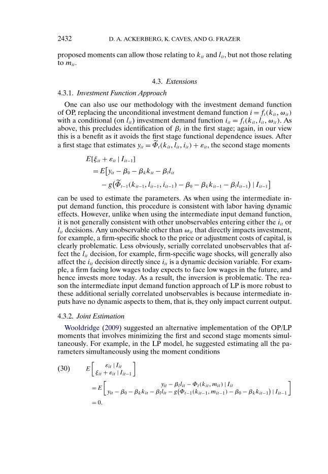
4.3.1. Investment Function Approach

One can also use our methodology with the investment demand functionof OP, replacing the unconditional investment demand function i = ft(kit�ωit)with a conditional (on lit) investment demand function iit = ft(kit� lit�ωit). Asabove, this precludes identification of βl in the first stage; again, in our viewthis is a benefit as it avoids the first stage functional dependence issues. Aftera first stage that estimates yit = Φ̃t(kit� lit� iit)+ εit , the second stage moments

E[ξit + εit | Iit−1]=E

[yit −β0 −βkkit −βllit

− g(Φ̃t−1(kit−1� lit−1� iit−1)−β0 −βkkit−1 −βllit−1

) | Iit−1

]can be used to estimate the parameters. As when using the intermediate in-put demand function, this procedure is consistent with labor having dynamiceffects. However, unlike when using the intermediate input demand function,it is not generally consistent with other unobservables entering either the iit orlit decisions. Any unobservable other than ωit that directly impacts investment,for example, a firm-specific shock to the price or adjustment costs of capital, isclearly problematic. Less obviously, serially correlated unobservables that af-fect the lit decision, for example, firm-specific wage shocks, will generally alsoaffect the iit decision directly since iit is a dynamic decision variable. For exam-ple, a firm facing low wages today expects to face low wages in the future, andhence invests more today. As a result, the inversion is problematic. The rea-son the intermediate input demand function approach of LP is more robust tothese additional serially correlated unobservables is because intermediate in-puts have no dynamic aspects to them, that is, they only impact current output.

4.3.2. Joint Estimation

Wooldridge (2009) suggested an alternative implementation of the OP/LPmoments that involves minimizing the first and second stage moments simul-taneously. For example, in the LP model, he suggested estimating all the pa-rameters simultaneously using the moment conditions

E

[εit | Iit

ξit + εit | Iit−1

](30)

= E

[yit −βllit −Φt(kit �mit) | Iit

yit −β0 −βkkit −βllit − g(Φt−1(kit−1�mit−1)−β0 −βkkit−1

) | Iit−1

]= 0�


As pointed out by Wooldridge, there are several advantages to this approach.First, the joint approach avoids the functional dependence issue describedabove. Even if lit is functionally dependent on mit , kit , and t, βl might beidentified by the second set of moments (however, the nonparametric non-identification arguments of Gandhi, Navarro, and Rivers (2014) might applyto such an approach). Other advantages of the joint approach are potentialefficiency gains, and simpler standard error calculations. There are also dis-advantages of the joint approach; in particular, the joint approach requires anonlinear search over β0, βk, βl, and the parameters representing the two un-known functions Φt and g. This is more time consuming and likely more errorprone than the two-stage approach, which can often be performed with a non-linear search over just βk and βl (if Φt and g are represented by polynomials,the first stage can be estimated using OLS, and in the second stage, OLS canbe used to concentrate out the parameters of g—see the Appendix).

Note that if one applied the idea of Wooldridge directly to our proposedmoments (26) and (27), one gets something slightly different than (30), that is,

E

[εit | Iit

ξit + εit | Iit−1

](31)

=E

[yit − Φ̃t (kit � lit �mit ) | Iit

yit −β0 −βkkit −βllit − g(Φ̃t−1(kit−1� lit−1�mit−1)−β0 −βkkit−1 −βllit−1

) | Iit−1

]= 0�

Specifically, (30) is a restricted version of (31), a version where Φ̃t(kit� lit�mit)is assumed to be linear in lit . The distinction also exactly corresponds to ourdistinction between moments based on the unconditional intermediate inputdemand function (the Wooldridge moments (30)) and our moments based onthe conditional intermediate input demand function (31). For the same rea-sons as discussed above, we prefer (31) because it makes fewer assumptions—(31) allows serially correlated unobserved wage shocks, allows dynamic laborwith adjustment costs, and allows materials to be chosen after labor (more-over, these potential aspects of the data generating process help avoid the non-identification results of Gandhi, Navarro, and Rivers (2014)). On the otherhand, (30) does not allow this. One could also use the two sets of momentsto test this restriction; if one models and interprets Φ̃t as a flexible paramet-ric polynomial (rather than a nonparametric function), one could use a simpleWald or LR test for the restrictions that the linear coefficient on l in Φ̃(k� l�m)equals βl and all other coefficients involving l equal 0 (note that this is relatedto the overidentifying restrictions tests performed by OP and LP).

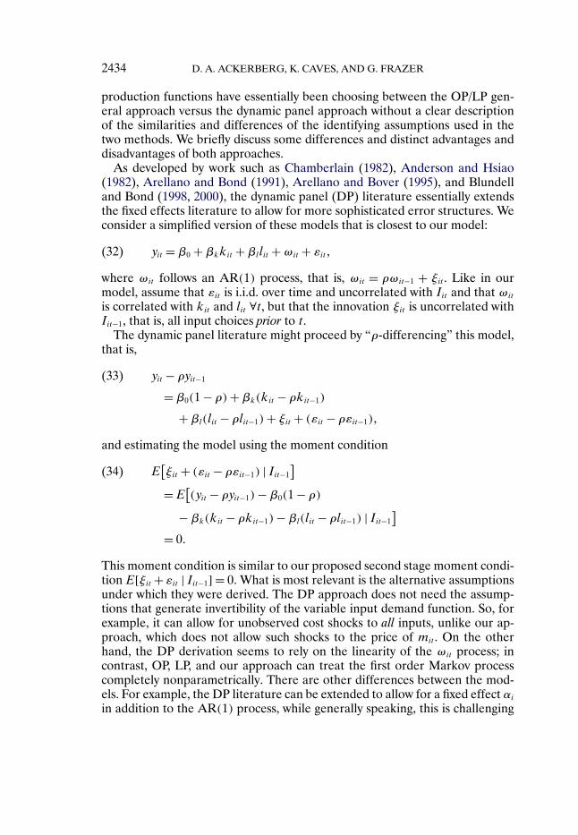
4.3.3. Relation to Dynamic Panel Methods

Interestingly, the form of our suggested estimators makes them fairly easy tocompare to estimators used in an alternative literature, the dynamic panel liter-ature. This is important because up to now, researchers interested in estimating


production functions have essentially been choosing between the OP/LP gen-eral approach versus the dynamic panel approach without a clear descriptionof the similarities and differences of the identifying assumptions used in thetwo methods. We briefly discuss some differences and distinct advantages anddisadvantages of both approaches.

As developed by work such as Chamberlain (1982), Anderson and Hsiao(1982), Arellano and Bond (1991), Arellano and Bover (1995), and Blundelland Bond (1998, 2000), the dynamic panel (DP) literature essentially extendsthe fixed effects literature to allow for more sophisticated error structures. Weconsider a simplified version of these models that is closest to our model:

yit = β0 +βkkit +βllit +ωit + εit�(32)

where ωit follows an AR(1) process, that is, ωit = ρωit−1 + ξit . Like in ourmodel, assume that εit is i.i.d. over time and uncorrelated with Iit and that ωit

is correlated with kit and lit ∀t, but that the innovation ξit is uncorrelated withIit−1, that is, all input choices prior to t.

The dynamic panel literature might proceed by “ρ-differencing” this model,that is,

yit − ρyit−1(33)

= β0(1 − ρ)+βk(kit − ρkit−1)

+βl(lit − ρlit−1)+ ξit + (εit − ρεit−1)�

and estimating the model using the moment condition

E[ξit + (εit − ρεit−1) | Iit−1

](34)

=E[(yit − ρyit−1)−β0(1 − ρ)

−βk(kit − ρkit−1)−βl(lit − ρlit−1) | Iit−1

]= 0�

This moment condition is similar to our proposed second stage moment condi-tion E[ξit + εit | Iit−1] = 0. What is most relevant is the alternative assumptionsunder which they were derived. The DP approach does not need the assump-tions that generate invertibility of the variable input demand function. So, forexample, it can allow for unobserved cost shocks to all inputs, unlike our ap-proach, which does not allow such shocks to the price of mit . On the otherhand, the DP derivation seems to rely on the linearity of the ωit process; incontrast, OP, LP, and our approach can treat the first order Markov processcompletely nonparametrically. There are other differences between the mod-els. For example, the DP literature can be extended to allow for a fixed effect αi

in addition to the AR(1) process, while generally speaking, this is challenging


in our context because it would tend to violate the scalar unobservable assump-tion. The DP literature also can potentially allow future values of the interme-diate input or investment variable to depend on past εit ’s, while our approachcannot. On the other hand, as elaborated on in OP, the scalar unobservable as-sumption of OP/LP and our approach makes it fairly straightforward to extendthe methodologies to address endogenous exit (selection) from a sample (seeOP); this would be considerably harder in the DP context. In summary, bothapproaches require strong (but different) assumptions. In some cases, a prioribeliefs about a particular production process and/or data considerations mayguide choices between the two approaches. In other cases, one may want totry both techniques. Finding that estimates are consistent across multiple tech-niques with different assumptions is surely more convincing than only usingone.

4.3.4. Units of Measure

The above discussion has implicitly assumed an “ideal” data scenario whereall the variables are measured in physical units that are equivalent across firms.While lit is often measured in physical units (number of workers, or numberof hours), output and inputs such as capital and materials are probably mostfrequently measured in monetary units. When output or an input is measuredin monetary values, there are a few things that must be considered to apply theabove techniques.

First, assume that firms are price takers in both input and output markets.The first question is whether the prices of equivalent inputs or output varyacross firms.12 If there is no variation in prices, then the monetary units arecomparable across firms and one can apply the above techniques straightfor-wardly. On the other hand, if the prices of those equivalent inputs (or output)do vary across firms, then the monetary units are not comparable across firms(see, e.g., Klette and Griliches (1996)). In this case, the price variation must beobserved for straightforward application of the above techniques. When theprice variation is observed, then one can easily divide by prices to obtain mea-sures of physical units and one can apply the above (note that the observedinput and output prices need to be included in the intermediate input (or in-vestment) demand function). Note that the observed input prices could alsobe used as additional instruments for the moment conditions under appropri-ate assumptions (e.g., that those input prices are exogenous); see, for example,Doraszelski and Jaumandreu (2013).

12When we describe measures of inputs and outputs as being equivalent across firms, we areruling out a situation where input or output price differences across firms reflect differencesin quality. If one thinks that quality differences are important, monetary measures of input oroutputs may be superior to (non-equivalent) physical measures, though as noted below, usingmonetary measures requires an assumption that firms face the same menu of prices (menu overdifferent quality levels).


Alternatively, consider a situation where firms face downward sloping outputdemand curves (and/or upward sloping input supply curves). In this case, onewill generally need to assume that firms are all facing identical demand/supplycurves; otherwise, firms will have different intermediate input (or investment)demand functions (i.e., the scalar unobservable Assumptions 4, 4b, or 4c willbe violated). But even if this is true, there is still a problem since firms willgenerally be operating on different points of those demand and supply curves.Because of the resulting price differences, monetary values of inputs or outputwill again generally not be comparable across firms. If one observes the pricedifferences of equivalent inputs or outputs, one can again construct measuresof equivalent physical units and apply the above. If one does not observe theprice differences, then other techniques are required—see Klette and Griliches(1996), De Loecker (2011), and De Loecker and Warzynski (2012) for recentmethodological advances for this situation.

5. MONTE CARLO EXPERIMENTS

The discussion above implies that whether OP, LP, or our procedure gener-ates consistent estimates of the production function parameters depends onthe underlying DGP. What we instead focus on in our Monte Carlo experi-ments is how the various procedures perform under misspecification. Specifi-cally, we consider misspecification where the intermediate input or investmentvariable is measured with error. In this case, none of the procedures produceconsistent estimates, but we illustrate (in at least one setup) that our proce-dure appears less affected by this misspecification than OP and LP. Note thatsince the original version of the paper, others have proposed newer methodsof explicitly addressing measurement error in inputs; Huang and Hu (2011)proposed a method to explicitly deal with such measurement error in these ap-proaches based on observing multiple proxies and deconvolution methods, andKim, Petrin, and Song (2013) also allowed for measurement error in capital.

Our Monte Carlo setup extends the work of Syverson (2001) and Van Biese-broeck (2007), who considered a simple dynamic model of firm investment andproduction that is analytically solvable (which considerably eases computationburden and reliability issues for Monte Carlo purposes). The parameters ofthe model were chosen to match a couple of key moments in the Chilean dataused by LP. The full model setup is described in the Appendix, but the basicsare as follows. Productivity follows a first order AR(1) process. Firms makeoptimal choices of investment in the capital stock to maximize the expected(discounted) value of future profits, where there are convex capital adjustmentcosts, and as above, the period-t capital stock is determined by investment att − 1 (i.e., Kit = (1 − δ)Kit−1 + Iit−1). Material inputs mit are chosen at t, whilelabor input lit is chosen either at t or at t − b (in the latter case, labor is cho-sen with only knowledge of ωit−b, not ωit). The production function is assumed


Leontief in (and proportional to) materials (as in Van Biesebroeck (2003), forexample), that is,

Yit = min{β0K

βkit L

βlit exp(ωit)�βmMit

}exp(εit)�

where β0 = 1, βk = 0�4, βl = 0�6, and βm = 1. Given that the Leontief first or-der condition holds, this means that we can proceed using the “structural valueadded” (see Gandhi, Navarro, and Rivers (2014)) (log) production function

yit = β0 +βkkit +βllit +ωit + εit �

The other free parameters of the model were chosen such that the steady stateof the model approximately matches the overall relationship between capitaland labor in the Chilean data used by LP. Specifically, in our baseline speci-fications, 95% of the variation in capital in the data is across-firm variation,and the R2 of a regression of capital on labor is approximately 0.5. Impor-tantly, to match these two “moments” of the Chilean data, we needed to allowunobserved heterogeneity across firms in capital adjustment costs (see the Ap-pendix for details). This violates the scalar unobservable assumption if one isusing the investment variable of OP, and highlights the advantages of the LPintermediate input variable approach over the investment variable approachas described earlier; that is, the intermediate input approach (either with theLP moments or with our moments) allows unobserved variation across firmsin investment prices or capital adjustment costs. As a result, we primarily com-pare results using LP with the intermediate input variable, to our approachalso using the intermediate input variable.

We consider two base DGPs. The first, DGP1, is favorable to our procedurein that we add aspects to the DGP under which our moments produce con-sistent estimates but the LP moments do not. First, we assume that firms facedifferent (unobserved to the econometrician) wages, where the wage processfor firm i follows an AR(1) process. Second, we assume labor is chosen at timet−b, where b = 0�5 and where ω follows an AR(1) process both between ωit−1

and ωit−b and between ωit−b and ωit . Details are in the Appendix. As discussedin Section 3, the reason that our moments produce consistent estimates in thisDGP is because we use the conditional (on lit) intermediate demand function,while LP does not.13

13Note that, along with the assumption that firms are price takers in input and output markets,this particular “proportional in Mit” Leontief specification avoids Gandhi, Navarro, and Rivers’s(2014) critique of using these techniques with Leontief production functions. More specifically,in this setup, capital and labor will not be idled unless the firm chooses to shut down (if the scaledprice of materials is somehow less than the price of output), and if the firm shuts down, it wouldpresumably not be in the data set. Moreover, there is not even this type of optimal shut down inour Monte Carlos, since there is no across-firm variation in the price of materials or output. Seethe Appendix for more details.


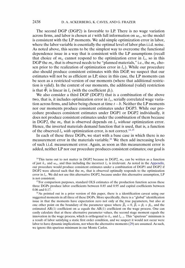
The second DGP (DGP2) is favorable to LP. There is no wage variationacross firms, and labor is chosen at t with full information on ωit , so the modelis consistent with the LP moments. We add simple optimization error in labor,where the labor variable is essentially the optimal level of labor plus i.i.d. noise.As noted above, this seems to be the simplest way to overcome the functionaldependence issue in a way that is consistent with the LP assumptions (recallthat choice of mit cannot respond to the optimization error in lit , so in thisDGP the mit that is observed needs to be “planned materials,” i.e., the mit cho-sen prior to the realization of optimization error in lit). While our procedurealso should produce consistent estimates with this DGP, we suspect that ourestimates will not be as efficient as LP, since in this case, the LP moments canbe seen as a restricted version of our moments (where that additional restric-tion is valid). In the context of our moments, the additional (valid) restrictionis that Φ̃t is linear in lit (with the coefficient βl).

We also consider a third DGP (DGP3) that is a combination of the abovetwo, that is, it includes optimization error in lit , serially correlated wage varia-tion across firms, and labor being chosen at time t−b. Neither the LP momentsnor our moments produce consistent estimates under DGP3. While our pro-cedure produces consistent estimates under DGP1 or DGP2 individually, itdoes not produce consistent estimates under the combination of them becausein DGP2, the mit that is observed depends on lit without optimization error.Hence, the inverted materials demand function that is used, that is, a functionof the observed lit with optimization error, is not correct.14,15

In each of these three DGPs, we start with a base case in which there is nomeasurement error in the materials variable.16 We then add increasing levelsof such i.i.d. measurement error. Again, as soon as this measurement error isadded, neither LP nor our procedure produces consistent estimates; our goal is

14This turns out to not matter in DGP2 because in DGP2, mit can be written as a functionof just kit and ωit , and thus including the incorrect lit is irrelevant. As noted in the Appendix,our procedure would produce consistent estimates under a combination of DGP1 and DGP2 ifDGP2 were altered such that the mit that is observed optimally responds to the optimizationerror in lit . We did not use this alternative DGP2, because under this alternative assumption, LPis not consistent.

15For comparison purposes, standard OLS estimates of the production function across thesethree DGPs produce labor coefficients between 0.85 and 0.95 and capital coefficients between0.06 and 0.17.

16As pointed out in a prior version of this paper, there is a identification caveat using oursuggested moments in all three of these DGPs. More specifically, there is a “global” identificationissue in that the moments have expectation zero not only at the true parameters, but also atone other point on the boundary of the parameter space where β̂k = 0, β̂l = βl + βk, and theestimated AR(1) coefficient on ω equals the AR(1) coefficient on the wage process. One caneasily calculate that at these alternative parameter values, the second stage moment equals theinnovation in the wage process, which is orthogonal to kit and lit−1. This “spurious” minimum isa result of labor satisfying a static first order condition, and we suspect it would not occur werelabor to have dynamic implications, nor when the alternative moments (29) are assumed. As such,we ignore this spurious minimum in our Monte Carlos.


TABLE I

MONTE CARLO RESULTSa

ACF LP

Meas.Error

βl βk βl βk

Coef. Std. Dev. Coef. Std. Dev. Coef. Std. Dev. Coef. Std. Dev.

DGP1—Serially Correlated Wages and Labor Set at Time t − b0.0 0.600 0.009 0.399 0.015 0.000 0.005 1.121 0.0280.1 0.596 0.009 0.428 0.015 0.417 0.009 0.668 0.0190.2 0.602 0.010 0.427 0.015 0.579 0.008 0.488 0.0150.5 0.629 0.010 0.405 0.015 0.754 0.007 0.291 0.012

DGP2—Optimization Error in Labor0.0 0.600 0.009 0.400 0.016 0.600 0.003 0.399 0.0130.1 0.604 0.010 0.408 0.016 0.677 0.003 0.332 0.0110.2 0.608 0.011 0.410 0.015 0.725 0.003 0.289 0.0100.5 0.620 0.013 0.405 0.017 0.797 0.003 0.220 0.010

DGP3—Optimization Error in Labor and Serially Correlated Wagesand Labor Set at Time t − b (DGP1 plus DGP2)

0.0 0.596 0.006 0.406 0.014 0.473 0.003 0.588 0.0160.1 0.598 0.006 0.422 0.013 0.543 0.004 0.522 0.0140.2 0.601 0.006 0.428 0.012 0.592 0.004 0.473 0.0120.5 0.609 0.007 0.431 0.013 0.677 0.005 0.386 0.012

a1000 replications. True values of βl and βk are 0.6 and 0.4, respectively. Standard deviations reported are ofparameter estimates across the 1000 replications.

to see how sensitive the various procedures are to the additional measurementerror. The top third of Table I contains results for DGP1; in the first row, thereis zero measurement error in the material input variable, and in later rows, thelevel of this measurement error is increased. Measurement error of, for exam-ple, 0.1 indicates that the measurement error is of a magnitude that increasesthe variance of mit by 10%.

The first row demonstrates that, as expected, even without measurementerror the LP moments do not produce what appear to be consistent estimates.On the other hand, our moment conditions do appear to produce consistentestimates when there is no measurement error. Interestingly, as we change thelevel of measurement error in mit , the LP estimate of the labor coefficientis considerably more sensitive, ranging from way below the true value of 0.6with no measurement error, to considerably above the true value when thereis lots of such error. Estimates using our moment conditions are again fairlystable, though there seems to be a small positive bias as the measurement errorincreases from 0.

The middle third of Table I contains results from DGP2. As noted above,with no measurement error, both our procedure and the LP procedure effec-tively find the true coefficients on labor and capital. Also as expected, the LPestimates are considerably more precise than those using our moments. How-


ever, as measurement error in materials is added, the LP labor coefficient in-creases and the LP capital coefficients decrease away from the true parameters.The capital parameter using our moments seems to be relatively unaffected bythe measurement error in materials, while the labor coefficients do move some-what. However, generally speaking, the LP coefficient estimates seem more af-fected by the measurement error than do the coefficient estimates based onour moments.

The last third of Table I contains results from DGP3. Again, neither proce-dure is consistent in this case, even without measurement error in mit . But with-out the measurement error, the estimates based on our moments are closer tothe truth than the LP estimates. Moreover, we again find that our estimates aremuch less sensitive than the LP estimates to measurement error. For βl and βk,our moments generate estimates that are at most only about 10% away fromthe truth. In contrast, the LP estimate of the labor coefficient, for example,varies between 0.47 and 0.68. These results suggesting that our moments aremore robust to misspecification than the LP moments seem consistent with re-sults in a working paper version of this paper. There, using the actual Chileandata, we found that while results using our moments were relatively robustacross a variety of intermediate input proxies (materials, electricity, fuels), re-sults using the LP moments were more variable.

Lastly, we tried the OP estimator using investment to recover unobservedproductivity. As noted previously, given our use of firm-specific capital adjust-ment costs to reproduce observed patterns in the data, OP will not be consis-tent under any of these DGPs. In fact, the misspecification due to the firm-specific adjustment costs seems to dwarf any misspecification due to measure-ment error (now in the investment variable). As a result, regardless of the levelof that measurement error or the specification, we obtain labor coefficients es-timates of approximately 0.82 to 0.87 (Table II). This again highlights how thegeneral idea of Levinsohn and Petrin to use the intermediate input to invertproductivity (particularly in the context of our alternative moment conditions)may be preferable to the original OP idea of using investment.

6. CONCLUSIONS

We argue that some popular production function estimation techniques in-troduced by Olley and Pakes (1996) and Levinsohn and Petrin (2003) maysuffer, at least conceptually, from a functional dependence problem. We pro-pose an alternative, though quite related, estimator that avoids this functionaldependence problem. The alternative estimator differs from OP and LP inthat it inverts input demand functions that are conditional on choice of laborinput (while OP/LP invert unconditional input demand functions). We showhow this allows for more general underlying DGPs than does LP, similarly tohow LP allowed for some more general DGPs than did OP. In comparison toWooldridge’s (2009) stacked version of LP’s moments (again based on uncon-ditional input demands), our moments based on conditional input demands


TABLE II

MONTE CARLO RESULTSa

OP

Meas.Error

βl βk

Coef. Std. Dev. Coef. Std. Dev.

DGP1—Serially Correlated Wages and Labor Set at Time t − b0.0 0.824 0.002 0.188 0.0040.1 0.836 0.002 0.179 0.0040.2 0.845 0.002 0.171 0.0030.5 0.865 0.002 0.151 0.003

a1000 replications. True values of βl and βk are 0.6 and 0.4, respectively. Standard deviations reported are ofparameter estimates across the 1000 replications.

are strictly less restrictive. Again, this means that our estimator is strictly moregeneral than that proposed by Wooldridge, for example, allowing unobservedheterogeneity in labor input prices across firms, allowing labor to have dynamicimplications, and allowing labor to possibly be chosen prior to materials witha different information set. As might be expected, this generality and robust-ness in comparison to Wooldridge and LP does come at an efficiency cost; thatis, when the assumptions behind the unconditional input demand function ap-proach are in fact correct, estimates based on our conditional approach are lessefficient. These findings are born out by Monte Carlo experiments that com-pare performance of the estimators under various DGPs that are sometimesconsistent with the assumptions behind the estimators and sometimes not.

APPENDIX: MONTE CARLO SETUP

We now describe our Monte Carlo setup. We consider a panel of 1000 firmsover 10 time periods. The parameters of the model are chosen such that thecapital and labor series approximate key aspects of the Chilean data used inLP. Specifically, in our baseline specifications, 95% of the variation in capitalin the data is across-firm variation (vs. within-firm variation), and the R2 of aregression of capital on labor is approximately 0.5.

A.1. Production Function and Productivity Shocks

We use a production function that is Leontief in the material input, that is,

Yit = min{β0K

βkit L

βlit e

ωit �βmMit

}eεit �(35)

where β0 = 1, βk = 0�4, βl = 0�6, and βm = 1. Note that in this specification,material input is proportional to output. This is perhaps the most natural Leon-


tief specification, corresponding to a situation where a specific, fixed amountof the material input needs to be used to produce one unit of output (e.g.,some specific amount of metal required to produce a can to hold food, someamount of wood required to produce an item). εit is mean 0 measurement er-ror with standard deviation 0.1 that is distributed i.i.d. over firms and time. Theproductivity shock ωit follows the AR(1) process

ωit = ρωit−1 + ξit�(36)

where ρ = 0�7. The variances of the normally distributed innovation ξit (σ2ξ )

and the initial value ωi0 (σ2ωi0

) are set such that the standard deviation of ωit isconstant over time and equal to 0.3.

A.2. Choice of Labor and Material Inputs

As described in Section 5, our specifications differ in how they model theDGP generating the labor (and material) inputs. In all specifications, we as-sume that labor and materials are not dynamic inputs, that is, a firm’s choice ofLit and Mit has no implication for profitability after period t. As noted in themain text, our procedure is consistent if labor has dynamic implications. Wedid not allow this in our Monte Carlos; for speed and reliability purposes, wewanted a model where the firms’ dynamic programming problem can be solvedanalytically. When the only dynamic input is capital, we can extend Syverson(2001) and Van Biesebroeck (2007) to obtain a model for which the optimalinvestment level can be solved analytically. An alternative would be to followBond and Söderbom (2005), allow dynamics (e.g., adjustment costs) in bothcapital and labor, and solve the model numerically.

We consider two main data generating processes. DGP1 allows there to befirm-specific (unobserved to the econometrician) wage shocks, and also allowsLit to be chosen prior to period t, that is, without full knowledge of ωit . DGP1is favorable to our procedure in that our conditional input demand approachproduces consistent estimates, but the LP unconditional approach does not. Incontrast, DGP2 does not allow firm-specific wage shocks, and Lit is chosen withknowledge of ωit . However, DGP2 does add optimization error to Lit (whilethere is no optimization error in Mit). DGP2 is favorable to LP, as the LPprocedure produces consistent estimates. While our procedure also producesconsistent estimates, we expect them to have higher standard errors than thosegenerated by LP.

More specifically, DGP1 first allows labor to be chosen at time period t − b(we set b = 0�5). We can think of decomposing the AR(1) process (36) intotwo subprocesses. First, ωit−1 evolves to ωit−b, at which point in time the firmchooses labor input (as a function of ωit−b). Then, after Lit is chosen, ωit−b


evolves to ωit . We use the following model of the evolution of ω between sub-periods:

ωit−b = ρ1−bωit−1 + ξAit �

(37)ωit = ρbωit−b + ξB

it �

Thus, when b > 0, firms have less than perfect information about ωit whenchoosing Lit , and when b increases, this information decreases. Note that thisis consistent with the AR(1) coefficient in (36) since ρ1−bρb = ρ. Also for con-sistency with (36), we impose that Var(ρbξA

it + ξBit )= Var(ξit) and that the vari-

ance of ξAit is such that the variance of ωit−b is constant over time. This defines

Var(ξAit ) ≡ σ2

ξAand Var(ξB

it ) ≡ σ2ξB

, and intuitively implies that σ2ξA

is decreas-ing in b and σ2

ξBis increasing in b. In DGP1, firms also face different wages

where the (ln) wage process for firm i follows an AR(1) process

ln(Wit)= 0�3 ln(Wit−1)+ ξWit �

where the variances of the normally distributed innovation ξWit (σ2

ξW) and the

initial value ln(Wi0) are set such that the standard deviation of ln(Wit) is con-stant over time and equal to 0.1. Relative to a baseline in which all firms facethe mean log wage in every period, this wage variation increases the within-firm, across-time, standard deviation of ln(Lit) by about 10%.

Given DGP1, firms optimally choose Lit to maximize expected profits bysetting (with the difference between the price of output and the price of thematerial input normalized to 1)

Lit = β1/(1−βl)

0 β1/(1−βl)

l W−1/(1−βl)it K

βk/(1−βl)it e

(1/(1−βl))(ρbωit−b+(1/2)σ2

ξB)�

Note that DGP1 is not subject to the critique of Gandhi, Navarro, and Rivers(2014) of Leontief production functions (as noted in footnote 13 of the mainpaper). They discussed how, in the context of a Leontief production function,for example,

Yit = min{β0K

βkit L

βlit e

ωit �m(Mit)}eεit �(38)

it is possible that the Leontief “first order condition”

m(Mit)= β0Kβkit L

βlit e

ωit(39)

might not hold. The intuition for their argument is as follows. Suppose Kit

and Lit are chosen prior to Mit being chosen. Suppose that between these twopoints in time, the price of Mit rises precipitously (and unexpectedly), such thatthe revenue from selling output does not even cover the cost of the materialinput required to produce that output (i.e., ignoring the “sunk” costs of already


purchased Kit and Lit). In this case, firms would not generally choose Mit tosatisfy (39), and thus the data could contain points where

Yit = β0Kβkit L

βlit e

ωit+εit �

invalidating all the above procedures. However, in our Monte Carlo setupwhere output is proportional to material input (i.e., m(Mit) = βmMit , whichcould be the most plausible Leontief specification for many material inputs),this is not a problem. This is because firms will either satisfy (39) or producezero output (the latter if the price of Mit unexpectedly rises enough after theother inputs are chosen), and if they produce zero, they will presumably notbe in the data set of firms that are operating and thus not be a problem forestimation. Moreover, in our Monte Carlos, the prices of material inputs (andoutput) are constant across firms anyway, so firms never want to let capital andlabor go unutilized and produce zero.17

In contrast to DGP1, in DGP2 firms face identical wages and Lit is chosen atperiod t (i.e., b = 0). These changes are needed to make the model consistentwith the assumptions of LP. Moreover, we need something to break the func-tional dependence issue, so we add optimization error to Lit . More specifically,let Lerr

it be the firm’s choice of labor including optimization error. We assumethat

Lerrit =Lite

ξlit �

where ξlit ∼ N(0�σ2

ξl) is optimization error that is distributed i.i.d. over firms

and time (and independent of everything else in the model). We set σξl = 0�37,which also increases the within-firm, across-time, standard deviation of ln(Lit)by about 10%.

Constructing this DGP such that LP produces consistent estimates is some-what subtle. If the firm observes Lerr

it prior to choosing the material input, theywill typically choose

Merrit = β0K

βkit L

errβlit eωit �

This is a problem if the econometrician observes Merrit as the material input

measure, as this would violate the scalar unobservable assumption of LP (As-sumption 4b). So instead we assume that the econometrician observes Mit in-stead of Merr

it , where

Mit = β0Kβkit L

βlit e

ωit �

17Note that in this example, a fully nonparametric first stage regression of Yit on Kit , Lit , andMit to recover εit is not strictly needed given the assumed Leontief functional form. For exam-ple, one could alternatively regress Yit on just Mit to recover εit , or similarly, use the LeontiefFOC directly. In our Monte Carlos, we do the fully general first stage (perhaps sacrificing someefficiency) because that corresponds to our more general procedure.


One interpretation of this is that, after observing ωit , firms commit to“planned” optimal Lit and Mit . However, workers are randomly sick, and whenmore workers are sick less materials are used, so that the firm ends up usingLerr

it and Merrit and producing18

Yit = β0Kβkit L

errβlit eωit eεit �

What the econometrician is assumed to observe are Yit , Kit , Lerrit , and Mit . The

interpretation of observing Mit is that what is reported in the data is planned(or ordered) materials, that is, prior to the realization of sick days and Lerr

it .In DGP2, both LP and our procedure produce consistent estimates. While

we do not present results for this, one can consider an alternative DGP2, callit DGP2b, where Merr

it is observed instead of Mit . In DGP2b, LP does not pro-duce consistent estimates, but our suggested procedure does (since conditionalon Lerr

it , the scalar unobservable assumption is not violated). We also considerthe combination of DGP1 and DGP2, that is, a DGP that includes across-firmwage variation, labor chosen at t − b, and optimization error in Lit . In thissetup, neither LP nor our procedure produces consistent estimates (see themain text for a discussion of why our procedure does not produce consistentestimates under DGP1 + DGP2, even though it provides consistent estimatesunder DGP1 or DGP2 separately). While we again do not present results, ourprocedure would produce consistent estimates under DGP1 + DGP2b, whileLP would not.

For all three DGPs (DGP1, DGP2, and DGP3 = DGP1 + DGP2), we ad-ditionally add various levels of measurement error to the observed materialinput. As noted in the main text, this renders both LP and our approach incon-sistent. However, we find that estimation based on the LP moments appearsto be more sensitive to this measurement error than does estimation based onour moments.

A.3. Investment Choice and Steady State

In contrast to non-dynamic labor and material inputs, we assume that capi-tal is a dynamic input. Specifically, capital is accumulated through investmentaccording to

Kit = (1 − δ)Kit−1 + Iit−1�

18In theory, the Leontief critique of GNR could apply here. For example, if between the pointin time in which Lit is chosen and Lerr

it is realized, there is a large enough unexpected positiveshock to the price of the material input, it is possible that if Lerr

it > Lit , the firm would not wantto increase material input levels over Mit , that is, the unexpected supply of labor would optimallygo unutilized. However, in our setup, there are no such shocks to the price of material input (oroutput), so everything is internally consistent. Note also that when the econometrician observesplanned materials, as in this DGP, one cannot simply estimate the model directly off the Leontieffirst order condition.


where (1−δ)= 0�8, and investment is subject to convex adjustment costs givenby

ci(Iit)= φi

2I2it �

where 1/φi is distributed lognormally across firms (but constant over time)with standard deviation 0.6. While the existence of this unobserved hetero-geneity in adjustment costs is consistent with the LP procedure and our pro-cedure, it is not consistent with the scalar unobservable assumption in the OPcontext. This renders OP estimates inconsistent in all our Monte Carlos. Weincluded it because, without this heterogeneity, it was extremely hard (in steadystate, see below) to match the within-firm versus across-firm variation in cap-ital and the correlation between capital and labor of the Chilean data sets asdiscussed above.19

As described by Syverson (2001) and Van Biesebroeck (2007), under theassumption of constant returns to scale, a pared-down version of the above canbe solved analytically using Euler equation techniques. We have verified thattheir analytic result can be generalized to allow for the extensions in the abovemodel, that is, persistent across-firm variation in wages, labor being chosen att − b, and optimization error in Lit . Specifically, a Euler equation approachimplies the following optimal investment rule (where β is the discount factor,set to 0.95 in our Monte Carlos):

Iit = β

φi

∞∑τ=0

(β(1 − δ)

)τ( βk

1 −βl

)β

1/(1−βl)

0

× [β

βl/(1−βl)

l e(1/2)β2

lσ2ξl −β

1/(1−βl)

l e(1/2)σ2

ξl]

× exp

{[(1

1 −βl

)ρτ+1ωit + −βl

1 −βl

ρτ+1W ln(Wit)

+ 12

( −βl

1 −βl

)2

σ2ξW

τ∑s=0

ρ2(τ−s)W + 1

2

(1

1 −βl

)2

ρ2b

(ρ2τσ2

ξa

+τ∑

s=1

ρ2(τ−s)σ2ξ

)+(

11 −βl

)(12σ2

ξb

)]}�

19Without heterogeneity in φi , the only way our DGPs can match 95% of the variation in Kit

being “across-firm variation” is by setting the persistence of the productivity process ωit extremelyhigh. But when this persistence is extremely high, it implies a very high correlation between Kit

and Lit which contradicts the R2 of a fixed effects regression of Lit on Kit of only about 50% inthe Chilean data, unless one includes unrealistic amounts of optimization error or wage variation.


Note that because of the constant returns to scale, optimal investment doesnot depend on current capital stock—the only firm-specific variables that itdepends on are ωit , φi, and ln(Wit) (the latter because it is serially correlatedover time).

For our experiments, we did not want our results to depend on an arbi-trary, exogenous, initial distribution of capital stock across firms (one wouldalso need to somehow specify correlations between Ki0 and (ωi0�φi� ln(Wi0)).Instead, we decided to take data from the steady state distribution of firms im-plied by our model. To do this, we simply started all firms with Ki0 = 0, andsimulated firms into the future. Our 10 periods of data are taken from a pointin time where the impact of the initial values appeared minimal, that is, thesteady state.

A.4. Estimation

We estimate the following Leontief-derived value-added production func-tion:

Yit = β0Kβkit L

βlit e

ωit eεit

(or in DGP2, the same with Lit replaced with Lerrit ). When we use our procedure

or LP, we use Mit to invert the productivity shock, and when we run OP, we useIit .20

For our procedure, our first stage is simply OLS of yit on kit , lit , and mit .More generally, one would want higher order polynomials in the explanatoryvariables, but because, in our setup, optimal mit is actually a linear function ofkit , lit , and ωit , we simply used a first order polynomial. In the second stage,our estimation is based on the following moments (where β̃0 = ln(β0)):

E

⎡⎢⎣(yit − β̃0 −βkkit −βllit(40)

− ρ · (Φ̃t−1(kit−1� lit−1�mit−1)− β̃0 −βkkit−1 −βllit−1

))⊗⎛⎜⎝ 1

kit

lit−1


⎞⎟⎠⎤⎥⎦

= 0�

20As noted, one could also use our moments along with Iit as the variable to recover the pro-ductivity shock, but because of the unobserved heterogeneity in φi in our Monte Carlo setup, thiswould, like OP, not generate consistent estimates.


However, to reduce the dimension of the nonlinear search (and presumablyincrease speed and reliability for our experiments), we do not use these mo-ments directly. Instead we “concentrate-out” two of the parameters β̃0 and ρ.More specifically, for a hypothetical guess of the parameters βk and βl, weconstruct

˜̂β0 +ωit(βk�βl)= ̂̃Φt(kit� lit�mit)−βkkit −βllit�

where, again, ̂̃Φt(kit� lit�mit) is the predicted value from the first stage. We

then regress ˜̂β0 +ωit(βk�βl) on ̂β̃0 +ωit−1(βk�βl), noting that the residualsof this regression are the implied values of the innovations in omega, that is,ξ̂it(βk�βl). Note that this regression implicitly makes these innovations meanzero and uncorrelated with ω̂it−1(βk�βl), so it is similar to enforcing the firstand fourth moments in (40). While generally one might want to do this re-gression using higher order polynomials in the explanatory variable, we againsimply do it linearly, since our true DGPs use a linear AR(1) process for ωit .We then search over βk and βl space to find β̂k and β̂l that minimize the fol-lowing moment conditions:

E

[̂ξit(βk�βl)⊗

(kit

lit−1

)]= 0�(41)

Our estimate of ρ is given by the slope coefficient of the regression of˜̂β0 +ωit(βk�βl) on ̂β̃0 +ωit−1(βk�βl) evaluated at β̂k and β̂l.For our LP estimates, we use the canned STATA routine (Petrin, Poi, and

Levinsohn (2004))), edited to again use linear approximations (since accord-ing to the DGP, the true functions were in fact linear). Our results were verysimilar when we used the default routine based on cubic approximations. Forour OP results, we also use the canned LP STATA routine modified to use theinvestment variable, but here we use the default cubic approximation, sincethe dynamic investment function is not linear. In the online supplemental ma-terials, we include GAUSS versions of these estimation routines (Ackerberg,Caves, and Frazer (2015)).

REFERENCES

ACKERBERG, D., L. BENKARD, S. BERRY, AND A. PAKES (2007): “Econometric Tools for Analyz-ing Market Outcomes,” in Handbook of Econometrics. Amsterdam: North-Holland. [2412]

ACKERBERG, D. A., K. CAVES, AND G. FRAZER (2015): “Supplement to ‘Identification Prop-erties of Recent Production Function Estimators’,” Econometrica Supplemental Material, 83,http://dx.doi.org/10.3982/ECTA13408. [2448]

ACKERBERG, D., X. CHEN, J. HAHN, AND Z. LIAO (2014): “Asymptotic Efficiency of Semipara-metric Two-Step GMM,” Review of Economic Studies, 81 (3), 919–943. [2419]

AI, C., AND X. CHEN (2003): “Efficient Estimation of Models With Conditional Moment Restric-tions Containing Unknown Functions,” Econometrica, 71 (6), 1795–1843. [2419,2423]

http://www.e-publications.org/srv/ecta/linkserver/setprefs?rfe_id=urn:sici%2F0012-9682%28201511%2983%3A6%3C2411%3AIPORPF%3E2.0.CO%3B2-G

http://dx.doi.org/10.3982/ECTA13408

http://www.e-publications.org/srv/ecta/linkserver/openurl?rft_dat=bib:3/2&rfe_id=urn:sici%2F0012-9682%28201511%2983%3A6%3C2411%3AIPORPF%3E2.0.CO%3B2-G





(2007): “Estimation of Possibly Misspecified Semiparametric Conditional Moment Re-striction Models With Different Conditioning Variables,” Journal of Econometrics, 141, 5–43.[2419]

ALVAREZ, R., AND R. LOPEZ (2005): “Exporting and Performance: Evidence From ChileanPlants,” Canadian Journal of Economics, 38 (4), 1384–1400. [2412]

ANDERSON, T. W., AND C. HSIAO (1982): “Formulation and Estimation of Dynamic Models UsingPanel Data,” Journal of Econometrics, 18, 47–82. [2414,2434]

ARELLANO, M., AND S. BOND (1991): “Some Tests of Specification for Panel Data: Monte CarloEvidence and an Application to Employment Equations,” The Review of Economic Studies, 58,277–297. [2414,2434]

ARELLANO, M., AND O. BOVER (1995): “Another Look at the Instrumental Variable Estimationof Error Components Models,” Journal of Econometrics, 68, 29–51. [2414,2434]

BASU, S., AND J. FERNALD (1997): “Returns to Scale in U.S. Production: Estimates and Implica-tions,” Journal of Political Economy, 105, 249–283. [2428]

BLALOCK, G., AND P. GERTLER (2004): “Learning From Exporting: Revisited in a Less Devel-oped Setting,” Journal of Development Economics, 75 (2), 397–416. [2412]

BLUNDELL, R., AND S. BOND (1998): “Initial Conditions and Moment Restrictions in DynamicPanel Data Models,” Journal of Econometrics, 87, 115–143. [2414,2434]

(2000): “GMM Estimation With Persistent Panel Data: An Application to ProductionFunctions,” Econometric Reviews, 19, 321–340. [2414,2434]

BOND, S., AND M. SÖDERBOM (2005): “Adjustment Costs and the Identification of Cobb–DouglasProduction Functions,” Working Paper Series No. 05/04, The Institute for Fiscal Studies. [2428,

2442]BRUNO, M. (1978): “Duality, Intermediate Inputs, and Value-Added,” in Production Economics:

A Dual Approach to Theory and Applications, Vol. 2, ed. by M. Fuss and D. McFadden. Amster-dam: North-Holland, Chapter 1. [2428]

CHAMBERLAIN, G. (1982): “Multivariate Regression Models for Panel Data,” Journal of Econo-metrics, 18, 5–46. [2414,2434]

CHEN, X., J. HAHN, Z. LIAO, AND G. RIDDER, (2013): “Asymptotic Properties of NonparametricTwo-Step Sieve Estimates,” Report, UCLA. [2419]

CHRISTENSEN, L. R., AND W. H. GREENE (1976): “Economies of Scale in U.S. Electric PowerGeneration,” Journal of Political Economy, 84 (4), 655–676. [2411,2415]

CHRISTENSEN, L. R., D. W. JORGENSON, AND L. J. LAU (1973): “Transcendental LogarithmicProduction Frontiers,” Review of Economics and Statistics, 55 (1), 28–45. [2411,2415]

CRISCUOLO, C., AND R. MARTIN (2009): “Multinationals and U.S. Productivity Leadership: Evi-dence From Great Britain,” Review of Economics and Statistics, 91 (2), 263–281. [2412]

DE LOECKER, J. (2011): “Product Differentiation, Multi-Product Firms and Estimating the Im-pact of Trade Liberalization on Productivity,” Econometrica, 79 (5), 1407–1451. [2436]

DE LOECKER, J., AND F. WARZYNSKI (2012): “Markups and Firm-Level Export Status,” AmericanEconomic Review, 102 (6), 2437–2471. [2436]

DIEWERT, W. E. (1978): “Hick’s Aggregation Theorem and the Existence of a Real Value AddedFunction,” in Production Economics: A Dual Approach to Theory and Practice, Vol. 2, ed. byM. Fuss and D. McFadden. Amsterdam: North-Holland, Chapter 1. [2428]

DOLLAR, D., M. HALLWARD-DREIMEIER, AND T. MENGISTAE (2005): “Investment Climate andFirm Performance in Developing Countries,” Economic Development and Cultural Change, 54(1), 1–31. [2412]

DORASZELSKI, U., AND J. JAUMANDREU (2013): “R&D and Productivity: Estimating Endoge-nous Productivity,” Review of Economic Studies, 80, 1338–1383. [2418,2422,2428,2435]

FERNANDES, A. (2007): “Trade Policy, Trade Volumes and Plant-Level Productivity in ColombianManufacturing Industries,” Journal of International Economics, 71 (1), 52–71. [2412]

GANDHI, A., S. NAVARRO, AND D. RIVERS (2014): “On the Identification of Production Func-tions: How Heterogeneous Is Productivity,” Report, U–Wisconsin–Madison. [2428,2430,2433,

2437,2443]










































GRILICHES, Z., AND J. HAUSMAN (1986): “Errors in Variables in Panel Data,” Journal of Econo-metrics, 31, 93–118. [2414]

GRILICHES, Z., AND J. MAIRESSE (1998): “Production Functions: The Search for Identification,”in Econometrics and Economic Theory in the Twentieth Century: The Ragnar Frisch CentennialSymposium, ed. by S. Strøm. Cambridge, U.K.: Cambridge University Press. [2413-2415,2417,

2421]GRILICHES, Z., AND V. RINGSTAD (1971): Economies of Scale and the Form of the Production

Function. Amsterdam: North-Holland. [2414]HALL, R. E. (1988): “The Relation Between Price and Marginal Cost in U.S. Industry,” Journal

of Political Economy, 96, 921–947. [2414]HOCH, I. (1955): “Estimation of Production Function Parameters and Testing for Efficiency,”

Econometrica, 23, 325–326. [2411,2414](1958): “Simultaneous Equation Bias in the Context of the Cobb–Douglas Production

Function,” Econometrica, 26, 566–578. [2411](1962): “Estimation of Production Function Parameters Combining Time-Series and

Cross-Section Data,” Econometrica, 30, 34–53. [2411,2414]HUANG, G., AND Y. HU (2011): “Estimating Production Functions With Robustness Against

Errors in the Proxy Variables,” Report, Johns Hopkins University. [2436]KASAHARA, H., AND J. RODRIQUE (2008): “Does the Use of Imported Intermediates Increase

Productivity? Plant Level Evidence,” Journal of Development Economics, 87 (1), 106–118.[2412]

KIM, K., A. PETRIN, AND S. SONG (2013): “Estimating Production Functions With Control Func-tions When Capital Is Measured With Error,” Report, University of Chicago. [2436]

KLEIN, L. R. (1953): A Textbook of Econometrics. New York: Prentice-Hall. [2414]KLETTE, T. J., AND Z. GRILICHES (1996): “The Inconsistency of Common Scale Estimators When

Output Prices Are Unobserved and Endogenous,” Journal of Applied Econometrics, 11 (4),343–361. [2435,2436]

LEVINSOHN, J., AND A. PETRIN (2003): “Estimating Production Functions Using Inputs to Con-trol for Unobservables,” Review of Economic Studies, 70, 317–342. [2411,2413,2440]

MARSCHAK, J., AND W. H. ANDREWS JR. (1944): “Random Simultaneous Equations and theTheory of Production,” Econometrica, 12, 143–205. [2411,2414]

MCELROY, M. B. (1987): “Additive General Error Models for Production, Cost, and DerivedDemand or Share Systems,” Journal of Political Economy, 95 (4), 737–757. [2411,2415,2417,

2418,2429]MUNDLAK, Y. (1961): “Empirical Production Function Free of Management Bias,” Journal of

Farm Economics, 43, 44–56. [2411,2414](1963): “Estimation of Production and Behavioral Functions From a Combination of

Cross-Section and Time-Series Data,” in Measurement in Economics, ed. by C. Christ et al.Stanford, CA: Stanford University Press, 138–166. [2411,2414]

(1996): “Production Function Estimation: Reviving the Primal,” Econometrica, 64 (2),431–438. [2411,2424]

MUNDLAK, Y., AND I. HOCH (1965): “Consequences of Alternative Specifications in Estimationof Cobb–Douglas Production Functions,” Econometrica, 33, 814–828. [2411,2414]

NERLOVE, M. (1963): “Returns to Scale in Electricity Supply,” in Measurement in Economics, ed.by C. Christ et al. Stanford: Stanford University Press, 167–200. [2414]

OLLEY, S., AND A. PAKES (1996): “The Dynamics of Productivity in the TelecommunicationsEquipment Industry,” Econometrica, 64, 1263–1295. [2411,2413,2440]

OZLER, S., AND K. YILMAZ (2009): “Productivity Response to Reduction in Trade Barriers: Ev-idence From Turkish Manufacturing Plants,” Review of World Economics, 145 (2), 339–360.[2412]

PAKES, A., AND S. OLLEY (1995): “A Limit Theorem for a Smooth Class of Semiparametric Esti-mators,” Journal of Econometrics, 65, 295–332. [2421]






































PANZAR, J. (1989): “Technological Determinants of Firm and Industry Structure,” in Handbookof Industrial Organization, Vol. 1, ed. by R. Schmalensee and R. Willig. Amsterdam: North-Holland, 3–59. [2411]

PAVCNIK, N. (2002): “Trade Liberalization Exit and Productivity Improvements: Evidence FromChilean Plants,” Review of Economic Studies, 69, 245–276. [2411,2412]

PETRIN, A., B. POI, AND J. LEVINSOHN (2004): “Production Function Estimation in Stata UsingInputs to Control for Unobservables,” The Stata Journal, 4, 113–123. [2448]

ROBINSON, P. M. (1988): “Root-N-Consistent Semiparametric Regression,” Econometrica, 56,931–954. [2423]

SIVADASAN, J. (2009): “Barriers to Competition and Productivity: Evidence From India,” B.E.Journal of Economic Analysis & Policy, 9 (1), Article 42. [2412]

SLADE, M. (1989): “Modeling Stochastic and Cyclical Components of Technical Change: An Ap-plication of the Kalman Filter,” Journal of Econometrics, 41, 363–383. [2411]

SOLOW, R. M. (1957): “Technical Change and the Aggregate Production Function,” Review ofEconomics and Statistics, 39, 312–320. [2414]

SYVERSON, C. (2001): “Market Structuure and Productivity,” Ph.D. Dissertation, University ofMaryland. [2436,2442,2446]

TOPALOVA, P., AND A. KHADEWAL (2011): “Trade Liberalization and Firm Productivity: The Caseof India,” Review of Economics and Statistics, 93 (3), 995–1009. [2412]

VAN BIESEBROECK, J. (2003): “Productivity Dynamics With Technology Choice: An Applicationto Automobile Assembly,” Review of Economic Studies, 70 (1), 167–198. [2437]

(2007): “Robustness of Productivity Estimates,” The Journal of Industrial Economics, 55,529–569. [2436,2442,2446]

WOOLDRIDGE, J. (2009): “On Estimating Firm-Level Production Functions Using Proxy Vari-ables to Control for Unobservables,” Economics Letters, 104 (3), 112–114. [2413,2419,2432,

2440]

Dept. of Economics, University of Michigan, Ann Arbor, MI 48109, U.S.A.;[email protected],

Economists Inc., Washington, DC 20037, U.S.A.; [email protected],and

Dept. of Management, University of Toronto Scarborough, Toronto, ON M1C1A4, Canada, Rotman School of Management, University of Toronto, Toronto,ON M5S 3E6, Canada, and School of Public Policy and Governance, Universityof Toronto, Toronto, ON M5S 3K9, Canada; [email protected].

Manuscript received April, 2015; final revision received June, 2015.


http://www.e-publications.org/srv/ecta/linkserver/openurl?rft_dat=bib:53/n2&rfe_id=urn:sici%2F0012-9682%28201511%2983%3A6%3C2411%3AIPORPF%3E2.0.CO%3B2-G









mailto:[email protected]




http://www.e-publications.org/srv/ecta/linkserver/openurl?rft_dat=bib:53/n2&rfe_id=urn:sici%2F0012-9682%28201511%2983%3A6%3C2411%3AIPORPF%3E2.0.CO%3B2-G










Date post:	25-Apr-2018
Category:	Documents
Upload:	trinhhanh
View:	219 times
Download:	2 times

Econometrica, Vol. 83, No. 6 (November, 2015),...

Documents