Econometrics and Machine Learning - INSEE

147ECONOMIE ET STATISTIQUE / ECONOMICS AND STATISTICS N° 505‑506, 2018

Received on 2 September 2017, accepted after revision on 29 May 2018 Translated from the original version: “Économétrie et Machine Learning”

Econometrics and Machine LearningArthur Charpentier*, Emmanuel Flachaire** and Antoine Ly***

Abstract – On the face of it, econometrics and machine learning share a common goal: to build a predictive model, for a variable of interest, using explanatory variables (or features). However, the two fields have developed in parallel, thus creating two different cultures. Econometrics set out to build probabilistic models designed to describe economic phenomena, while machine learning uses algorithms capable of learning from their mistakes, generally for classification purposes (sounds, images, etc.). Yet in recent years, learning models have been found to be more effective than traditional econometric methods (the price to pay being lower explanatory power) and are, above all, capable of handling much larger datasets. Given this, econometricians need to understand what the two cultures are, what differentiates them and, above all, what they have in common in order to draw on tools developed by the statistical learning community with a view to incorporating them into econometric models.

Codes JEL / JEL Classification : C18, C52, C55Keywords: learning, Big Data, econometrics, modelling, least squares

Pour citer cet article: Charpentier, A., Flachaire, E. & Ly, A. (2018). Econometrics and Machine Learning. Economie et Statistique / Economics and Statistics, 505‑506, pp. 147–169. https://doi.org/10.24187/ecostat.2018.505d.1970

* University of Rennes 1 & CREM (arthur.charpentier@univ‑rennes1.fr)** Aix‑Marseille University, AMSE, CNRS & EHESS (emmanuel.flachaire@univ‑amu.fr)*** University of Paris‑Est ([email protected])

Reminder:

The opinions and analyses in this article are those of the author(s) and do not necessarily reflect their institution’s or Insee’s views.

ECONOMIE ET STATISTIQUE / ECONOMICS AND STATISTICS N° 505-506, 2018148

by contrast, nonparametric models are often built based almost exclusively on data (i.e. no distribution hypothesis), and the meta‑ parameters used (tree‑depth, penalty parame‑ter, etc.) are optimised by cross‑validation.1

Beyond the foundations, while the (often asymptotic) properties of θ (viewed as a ran‑dom variable, thanks to the underlying sto‑chastic representation) have been extensively studied in econometrics, statistical learning focuses to a greater extent on the properties of the optimal m ⋅( ) based on a criterion that remains to be defined, or even simply m xi

( ) for observations i deemed to be of interest for example in a test population. The problem of the choice of model is also viewed from a somewhat different perspective. Following Goodhart’s law (“When a measure becomes a target, it ceases to be a good measure”), the goodness‑of‑fit of a model is penalised after the fact in econometrics by its complexity in the validation or selection phase, while in statistical learning it is the objective function which takes account of the penalty.

From High Dimension to Big Data

In this paper, a variable will be a vector of n, such that by concatenating the variables, they can be stored in a matrix X , of size n p× , with n and p being potentially large.2 The fact that n is large is not a problem in itself. Many theorems in econometrics and statistics are obtained when n → ∞. By contrast, the fact that p is large is problematic, particularly if p n> .

Portnoy (1988) showed that the maximum likelihood estimator retains the asymptotic normality property if p remains small in relation to n (p n2 0/ → where n p, → ∞). Indeed, it is not uncommon to speak of high dimension when p n> . Another important concept is the idea of “sparsity”, which is based not on the dimension p but on the actual dimension, in other words the number of truly

1. The term “classification” will be used when is a set of classes, typi‑cally a binary classification, = { }0 1, , corresponding to the outcome of an indicator variable. The term is less dated than “discrimination” and more general than the determination of a “score” (often an intermediate step). It should not be confused with unsupervised classification (such as “ascend‑ing hierarchical classification”), which involves the creation of homogene‑ous classes based on a similarity measure (in this case, the term “creation or construction of classes” or “clusters” is sometimes used).2. Extensions are possible with MRI‑type images as predictive variables, or climate data with maps as predictive variables. It is possible fall back on the typical case of data in the form of vectors by using the Tucker decom‑position (Kolda & Bader, 2009).

The earliest use of quantitative techniques in economics probably dates back to the

sixteenth century (Morgan, 1990). However, it was not until the twentieth century that the term “econometrics” was first used, giving birth to the Econometric Society in 1933. Machine learning techniques are more recent. It was Arthur Samuel, widely regarded as the father of the first self‑learning programme, who first coined the term “machine learning”, which he defined as “a field of study that gives a computer the ability without being explic‑itly programmed” (Samuel, 1959). Among the earliest techniques are Hebb’s cell assembly theory (Hebb, 1949) (which later gave birth to the “perceptron” in the 1950s, and then to neural networks), with Widrow and Hoff (1960) demonstrating, around fifteen years later, the links with least‑squares methods, the SVM (support vector machine) and, more recently, boosting methods. While the two communities have developed in parallel, big data require links to be built between the two approaches by bridging the “two cultures” referred to by Breiman (2001a), contrasting mathematical statistics, which may be likened to traditional econometrics (Aldrich, 2010), with compu‑tational statistics and machine learning more generally.

Econometrics and supervised statistical learning techniques are similar, while also being very different. To start with, the two appear similar, with both using a database (or data table), i.e. observations y xi i,( ){ }, with i n= 1, ,

, xip∈ ⊂ and yi ∈ . If

yi is qualitative, we speak of a classification problem,1 and, otherwise, of a regression prob‑lem. The two approaches also share common ground at the other end since, in both cases, the aim is to build a “model”, i.e. a function m : which will be interpreted as a prediction.

However, there are significant differences in between. Historically, econometric models have been based on economic theory, gene‑rally with parametric models. Traditional sta‑tistical inference methods (such as maximum likelihood and the method of moments) are thus used to estimate the values of a vector of parameters θ , in a parametric model mθ ⋅( ), by a value θ. As in statistics, unbiased estimators are important since a lower bound on the vari‑ance can be obtained (Cramér‑Rao bound). Asymptotic theory plays an important role (Taylor expansions, law of large numbers and central limit theorem). In statistical learning,

ECONOMIE ET STATISTIQUE / ECONOMICS AND STATISTICS N° 505-506, 2018 149

Econometrics and Machine Learning

important variables. It is thus possible to have p n> while having convergent estimators.

The high dimension can be frightening because of the curse of dimensionality (Bellman, 1957). The volume of the unit sphere, in dimension p, tends towards 0 when p → ∞. In such cases, the space is said to be “parsimonious” – i.e. the likelihood of finding a point close to another becomes increasingly small (we may even speak of a “sparse” space). While the idea of reducing the dimension by using a principal component analysis may seem attractive, the analysis suffers from a number of flaws in high dimension. The solution often revolves around the selection of variables (which raises the problem of multiple tests or computational time).

To use the terminology of Buhlmann & van de Geer (2011), the problems highlighted here correspond to those encountered in high dimension, an essentially statistical prob‑lem. From a computational perspective, we may go a little further, with truly Big Data. In the foregoing, the data were stored in a matrix X , of size n p× . There can be issues with storing such a matrix or even with using a matrix widely used in econometrics, X XT

(n n× ). The first‑order condition of the lin‑ear model is associated with the solution to X X yT β −( ) = 0. In reasonable dimension, the Gram‑Schmidt decomposition is used. In high dimension, the numerical descent and gra‑dient methods may be used, where the gradient is approximated by subsampling (Zinkevich et al., 2010). This computational dimension is often overlooked, despite the fact that it has been the basis of a significant number of meth‑odological advances in econometrics.

Nonparametric and Computational Statistics

The purpose of this paper is to explain the major differences between econometrics and statistical learning, which correspond to the cultures alluded to by Breiman (2001a) in referring, in the context of statistical model‑ling, to the data modelling culture (based on a stochastic model, such as logistic regression or a Cox model) and the algorithmic model‑ling culture (based on the implementation of an algorithm, such as random forests or sup‑port vector machines; for a complete list, see Shalev‑Shwartz & Ben‑David, 2014). However, the boundary between the two is blurred. At the intersection, we find, for

example, nonparametric econometrics, which is based on a probabilistic model (like econo‑metrics) while focusing to a greater extent on algorithms and their performance rather than on asymptotic theorems.

Some Machine Learning Tools

Neural Networks

Neural networks are semiparametric models. Nevertheless, this family of models can be approached in the same way as nonparametric models: the structure of neural networks (pre‑sented below) can be modified to extend the class of functions used to approximate a var‑iable of interest. More specifically, Cybenko (1989) showed that the set of neural functions is dense in the space of continuous functions on a compact space. In other words, we have a theoretical framework which guarantees a form of universal approximation. It also requires defining a neuron and emphasises the existence of a sufficient number of neurons to approximate any continuous function on a compact domain. Thus, a continuous phe‑nomenon can be approximated by a sequence of neurons: this sequence is referred to as a “single‑layer neural network”. While the uni‑versal approximation theorem was demon‑strated in 1989, the first functional artificial neuron was introduced by Franck Rosenblatt in the mid‑twentieth century in Rosenblatt (1958). Referred to now as “basic neuron”, this neuron is known as “Perceptron”. In its earliest uses, it was used to determine the gen‑der of an individual presented in a photo. It introduced the first mathematical representa‑tion of a biological neuron:

- The synapses transmitting the information to the cell are represented by a real vector. The dimension of the input vector of the neuron (which is none other than a function) corre‑sponds biologically to the number of synaptic connections;

- Each signal transmitted by a synapse is then analysed by the cell. Mathematically, the schema is expressed by weighting the different components of the input vector;

- Depending on the information acquired, the neuron decides whether or not to resend a sig‑nal. The phenomenon is replicated by introduc‑ing an activation function. The output signal


is modelled by a real number computed as an image by the activation function of the weighted input vector.

Thus, an artificial neuron is a semiparametric model. The choice of activation function is left to the user. A basic neuron may then be for‑mally defined by:

1. An input space , generally k with k ∈*;

2. An output space , generally or a finite set (typically 0 1,{ }, although here we prefer − +{ }1 1, );

3. A vector of parameters w p∈ ;

4. An activation function φ : → . Ideally, this function should be monotonic, derivable and bounded (here, “saturating”) to ensure cer‑tain convergence properties.

This last function φ is reminiscent of logistic or probit transformations, which are popular in econometrics (which are cumulative distri‑bution functions, of value in 0 1,[ ], ideal when is the set 0 1,{ }). For neural networks, pref‑erence is given to the hyperbolic tangent, the arctangent function or the sigmoid functions for classification problems on = − +{ }1 1, (the latter evoke the logistic transformation performed by econometricians). The term neu‑ron is used to refer to any application fw of in defined by:

y f x x xT= ( ) = ( ) ∀ ∈w wφ ,

For the perceptron, introduced by Rosenblatt (1958), a basic neuron is assimilated to the function:

y f x x xT= ( ) = ( ) ∀ ∈w signe w ,

According to this formalisation, many statis‑tical models, such as logistic regressions, may be viewed as neurons. Any GLM (Generalised Linear Model) could be interpreted as an arti‑ficial neuron where the activation function φ is none other than the inverse of the canonical link function. If g denotes the link function of the GLM, w the vector of parameters, y the variable to be explained and x the vector of explanatory variables of the same dimension as w:

g Y X x w xT( [ | ]) = =

We return to neural modelling by taking φ = −g 1. However, the chief difference

between GLMs and the neural model is that the latter requires no distribution hypothesis on Y X| (here there is no need to introduce a probabilistic model). Furthermore, when the number of neurons per layer increases, convergence is not necessarily guaranteed if the activation function does not verify cer‑tain properties (which is not the case for the majority of the canonical link functions of GLMs). However, neural network theory imposes additional mathematical constraints on the function g (detailed in Cybenko, 1989). Thus, for example, a logistic regression may be viewed as a neuron, whereas generalised linear regressions do not verify all the neces‑sary hypotheses.

To extend the analogy with the functioning of the nervous system, it is then possible to connect different neurons. We speak of a lay‑ered neural network structure. Each layer of neurons receives the same observation vector every time. To revert to a more econometric analogy, we might imagine an intermediate step, for example by not performing a regres‑sion on the raw variables x but a smaller set of orthogonal variables obtained based on a principal component analysis. Consider A as the matrix associated with this linear transfor‑mation, with A of size k p× if we wish to use the p first components. Take z as the trans‑formation of x, where z A xT= (z A xj j

T= ). One generalisation of the above model may be to posit:

y f x w z w A xT T T= ( ) = ( ) = ( ) ∀ ∈φ φ , x

where w p∈ . Here we have a linear transfor‑mation (by considering a principal component analysis), although we can imagine a generali‑sation with nonlinear transformations:

y f x F x xTA= ( ) = ( )( ) ∀ ∈φ w ,

where F is a function k p→ . It is the two‑layer neural network. More generally, in order to formalise the construction, the follow‑ing notations are introduced:

• K ∈*: number of layers;

• ∀ ∈{ }k K1, , pk represents the number of neurons in the layer k;

• ∀ ∈{ }k K1, , Wk denotes the matrix of the parameters associated with the layer k. More specifically, Wk is a matrix p pk k× −1 and for any ∈{ }1, pk , wk l

pk, ∈ − 1 denotes the weight



vector associated with the basic neuron l of the layer k;

• W W WK= { }1,.., denotes the set of parameters associated with the neural network;

• FWk p pk

k k: − →1 denotes the transfer func‑tion associated with the layer k. For the purpose of simplification, we may also write F k �;

• y kpk ∈ will represent the image vector of

the layer k K∈{ }1, , �;

• F F F FWK= =

1 will denote the transfer function associated with the global network. In this respect, if x ∈ , we may note y F xW = ( ).

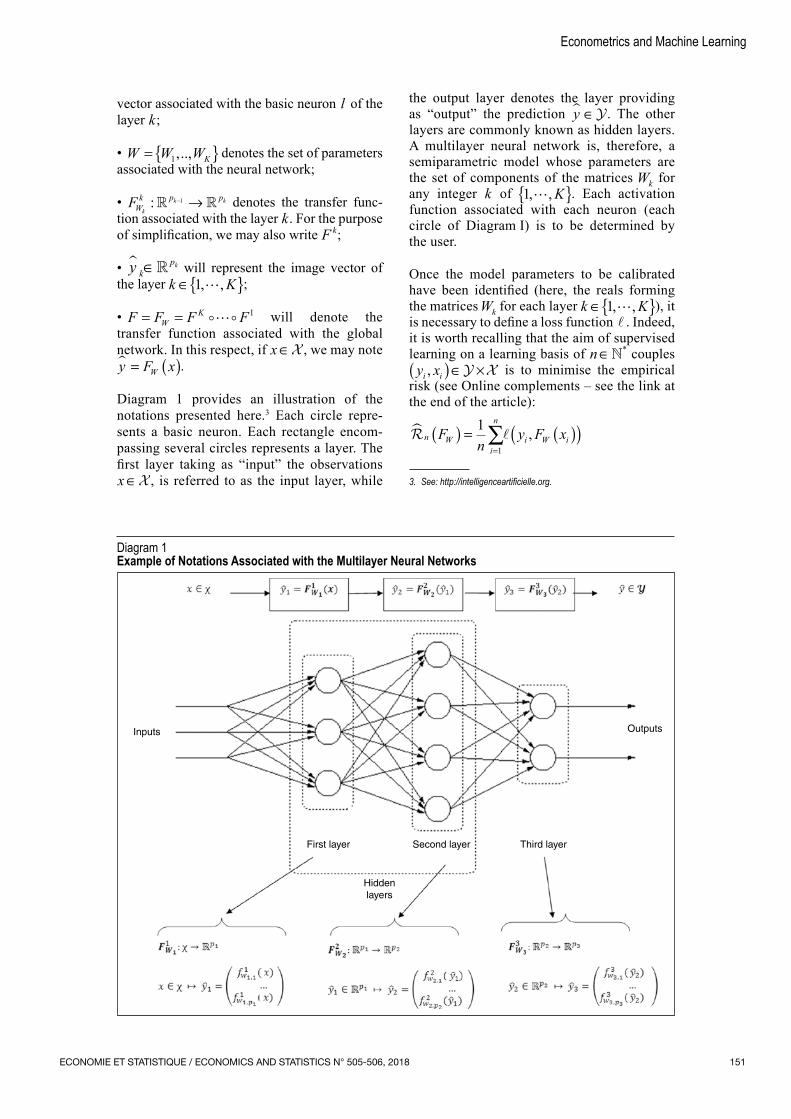
Diagram 1 provides an illustration of the notations presented here.3 Each circle repre‑sents a basic neuron. Each rectangle encom‑passing several circles represents a layer. The first layer taking as “input” the observations x ∈ , is referred to as the input layer, while

the output layer denotes the layer providing as “output” the prediction y∈ . The other layers are commonly known as hidden layers. A multilayer neural network is, therefore, a semiparametric model whose parameters are the set of components of the matrices Wk for any integer k of 1, , K{ }. Each activation function associated with each neuron (each circle of Diagram I) is to be determined by the user.3

Once the model parameters to be calibrated have been identified (here, the reals forming the matrices Wk for each layer k K∈{ }1, ,

), it is necessary to define a loss function . Indeed, it is worth recalling that the aim of supervised learning on a learning basis of n ∈* couples

y xi i,( )∈ × is to minimise the empirical risk (see Online complements – see the link at the end of the article):

n Wi

n

i W iFn

y F x( ) = ( )( )=∑1

1

,

3. See: http://intelligenceartificielle.org.

Diagram 1Example of Notations Associated with the Multilayer Neural Networks

Inputs

First layer Second layer Third layer

Hiddenlayers

Outputs

http://intelligenceartificielle.org


To illustrate this point, let us consider the following example, which will also serve to illustrate the approach adopted. Let us assume that we are observing a phenomenon through observations yi ∈ −[ ]1 1, . The aim is to explain this phenomenon based on the independant variables x which are assumed to have actual values. The “universal approximation theo‑rem” tells us that a single‑layer neural network should enable the phenomenon to be modelled (subject to it being continuous). However, the theorem provides no indication of convergence speed. The user retains control of the choice of structure, which may be a simple neuron whose activation function is the hyperbolic tangent function:

y w w x1 0 1= +( )tanh

where the parameters w w0 1, are to be opti‑mised in order to minimise the empirical risk over the learning data.

Based on the universal approximation theo‑rem, by adding several neurons, the error is expected to reduce. However, since the func‑tion to be estimated is not known, it can only be observed through the sample. Mechanically, learning‑based error decreases when parame‑ters are added. Error analysis by means of a test enables our ability to generalise to be assessed (Box 1).

A second model, which uses several neurons, may thus be considered. For example:

y w w w x w w w x

w w w xa b

c

2 0 1 2 3

4 5

= +( ) + +( )+ +( )

tanh tanh

tanh

where the parameters w w0 5,.., and w w wa b c, , are the parameters to be optimised. Calibrating a neural network thus amounts to reiterating these structural modification steps until the risk is minimised on a test basis.

For a fixed neural network structure (i.e. fixed number of layers, number of neurons per layer and activation functions), the programme there‑fore amounts to determining the set of parame‑ters W W WK

* ,...,= ( )1 in such a way that:

Wn

y F xW W W i

n

i W iK

*

,...,, .∈ ( )( )

=( ) =

∑argmin1

11

This formula underlines the importance of the choice of function . This loss function quantifies the average error of our model FW based on learning. A priori, can be chosen arbitrarily. However, from the point of view of working out an optimisation programme, sub‑differentiable and convex cost functions are preferable for guaranteeing the convergence of the optimisation algorithms. In addition to the quadratic loss function

22( ) ), (y y y y= − , tra‑

ditional loss functions include the hinge func‑tion − = −

( ) ), ( ,y y yymax 0 1 – and the logistic function − = − −

( ) ),y y e yylog(1 .

Neural networks were used very early on in economics and finance, notably on corporate defaults (Tam & Kiang, 1992; Altman et al., 1994) and, more recently, credit rating (Blanco et al., 2013; Khashman, 2011). However, structures such as those presented above are generally limited. Deep learning is more par‑ticularly characteristic of more complex neural networks (sometimes more than ten layers with hundreds of neurons per layer). Today, these

Box 1 – Learning and Test Samples

In the literature on learning, assessing the quality of a model based on the data used to build it says nothing about how the model will behave with new data. This is what is known as the “generalisation” problem. The traditional approach thus involves splitting the sample (of size n) in two: one part to train the model (the learn‑ing base, in‑sample, of size m) and another to test it (the test base, out‑of‑sample, of size n m− ). The lat‑ter allows for the measurement of a real predictive risk Let us suppose that the data are generated by a linear model y xi i

Ti= +β ε0 where the εi are realisations of

independent centred distributions. The in‑sample empir‑ical quadratic risk is:1

10 0

22

mx x x x

i

m

iT

iT

iT

iT

=∑ − = −( ) ( ) β β β β

for any observation i. If the residuals ε are Gaussian, this risk equals σ 2 p m/ , where � p is the size of the vec‑tors xi. By contrast, the out‑of‑sample empirical quad‑ratic risk is:

xT β β −( ) xT0

2

Where x is a new observation, which is independent of the others. We may note that:

x x x x X X xT T T Tβ β σ −( ) = −

0

22 1| ( )

and by integrating in relation to x:

x x x x x

xx

T T T T

T

β β β β

σ

− = − ( )( )=

( )[ ]

0

2

0

2

2

|trace X XT[[ ]( )−1

➔



structures are very popular in signal analysis (image, text, sound) because they are capable, based on a very large quantity of observations, of extracting information which humans are incapable of perceiving and to deal with non‑linear problems (LeCun et al., 2015).

Information extraction can, for example, be performed through convolution. As an unsu‑pervised procedure, it has produced excellent results in image analysis. In technical terms, this may be seen as a kernel‑based transfor‑mation (as used in SVM techniques; see next section). While an image may be viewed as a matrix, with each coordinate representing a pixel, a convolution amounts to applying a transformation to a point (or area) of this matrix, thereby producing a new datum. The

procedure can thus be repeated by applying different transformations (hence the notion of convolutional layers). The final vector obtained can then be fed into a neural model. More generally, a convolutional layer may be seen as a filter allowing the initial datum to be transformed.

One intuitive explanation for deep learning, and particularly deep networks, being so pow‑erful for describing complex relationships in data is their construction around a simple functional approximation and the use of a form of hierarchy (Lin et al., 2016). Nevertheless, deep learning models are more difficult to use since they require a significant degree of empi‑rical judgement. While open‑source libraries (Keras, Torch, etc.) currently allow more

The expression is then different from that obtained in‑sample, and by drawing on Groves & Rothenberg (1969), we can show that:

x x pm

T Tβ β σ − ≥( )0

22

Except for certain simple cases, there is no simple for‑mula. We may note, however, that if x ∼ ( ) 0 2,σ , then x xT follows a Wishart distribution, and:

x x pm p

T Tβ β σ −

=− −0

22

1Let us now consider the empirical version: if β is esti‑mated on the m first observations,

�IS

= −= +∑

i m

m

i iTy x

1

2[ ]β and �OS

= −= +∑

i m

n

i iTy x

1

2[ ]β

and as noted by Leeb (2008),

IS OS− ≈ ⋅2 ν where

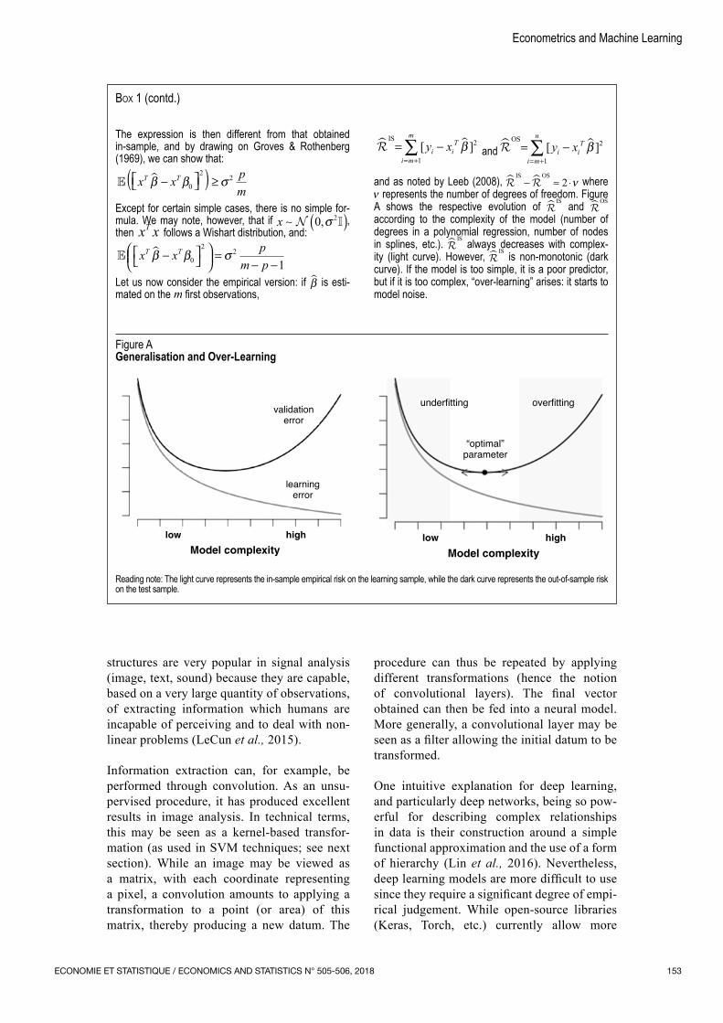
ν represents the number of degrees of freedom. Figure A shows the respective evolution of

IS and OS

according to the complexity of the model (number of degrees in a polynomial regression, number of nodes in splines, etc.).

IS always decreases with complex‑ity (light curve). However,

IS is non‑monotonic (dark curve). If the model is too simple, it is a poor predictor, but if it is too complex, “over‑learning” arises: it starts to model noise.

Box 1 (contd.)

Figure AGeneralisation and Over‑Learning

low

learningerror

validationerror

high

Model complexity

low

underfitting overfitting

high

Model complexity

“optimal”parameter

Reading note: The light curve represents the in‑sample empirical risk on the learning sample, while the dark curve represents the out‑of‑sample risk on the test sample.


readily for parallel computations by using, for example, GPUs (Graphical Processor Units), the user is still required to determine the struc‑ture of the most appropriate neural network.

Support Vector Machines

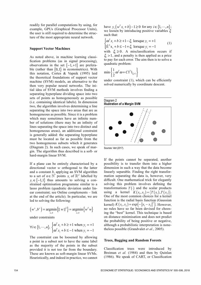
As noted above, in machine learning classi‑fication problems (as in signal processing), observations in the set − +{ }� , �1 1 are prefera‑ble (rather than 0 1,{ } in econometrics). With this notation, Cortes & Vapnik (1995) laid the theoretical foundations of support vector machine (SVM) models, an alternative to the then very popular neural networks. The ini‑tial idea of SVM methods involves finding a separating hyperplane dividing space into two sets of points as homogeneously as possible (i.e. containing identical labels). In dimension two, the algorithm involves determining a line separating the space into two areas that are as homogeneous as possible. Since it is a problem which may sometimes have an infinite num‑ber of solutions (there may be an infinity of lines separating the space into two distinct and homogeneous areas), an additional constraint is generally added: the separating hyperplane must be located as far as possible from the two homogeneous subsets which it generates (Diagram 2). In such cases, we speak of mar‑gin. The algorithm thus described is a soft‑ or hard‑margin linear SVM.

If a plane can be entirely characterised by a directional vector w orthogonal to the latter and a constant b, applying an SVM algorithm to a set of n∈* points xi of p labelled by yi ∈ −{ }1 1, thus amounts to solving a con‑strained optimisation programme similar to a lasso problem (quadratic deviation under lin‑ear constraint; see Online complements – link at the end of the article). In particular, we are led to solving the following:

ww w

,, ,

b w w wb b

T( ) = { } = { }argmin argmin

2

under constraints

∀ ∈{ }i n1, ,, ω

ω

Ti i

Ti i

x b yx b y

+ ≥ + = ++ ≤ − = −

� �� 1 11 1� when �� when �

The constraint can be loosened by allowing a point in a subset not to have the same label as the majority of the points in the subset provided it is not too far from the boundary. These are known as soft‑margin linear SVMs. Heuristically, and indeed in practice, we cannot

have y w x biT

i +( ) − ≥1 0 for any i n∈{ }1, ,;

we loosen by introducing positive variables ξ such that:

ω ξξ

Ti i i

i i

x b yb y

+ ≥ + − = ++ ≤ − + = −

� �� 1 11 1

� lorsque�É x � lorsque�T

i (1)

with ξi ≥ 0 . A misclassification occurs if ξi >1, and a penalty is then applied as a price to pay for each error. The aim then is to solve a quadratic problem:

min 12

1 1 1ω ωT TC+

>ξ

under constraint (1), which can be efficiently solved numerically by coordinate descent.

If the points cannot be separated, another possibility is to transfer them into a higher dimension in such a way that the data become linearly separable. Finding the right transfor‑mation separating the data is, however, very difficult. One mathematical trick for elegantly solving this problem involves defining the transformations T ⋅( ) and the scalar products using a kernel K x x T x T x1 2 1 2, ,( ) = ( ) ( ) . One of the most common choices for a kernel function is the radial basis function (Gaussian kernel) K x x x x1 2 1 2

2,( ) = − −( )exp . However, no rules have so far been devised for choos‑ing the “best” kernel. This technique is based on distance minimisation and does not predict the probability of being positive or negative, although a probabilistic interpretation is none‑theless possible (Grandvalet et al., 2005).

Trees, Bagging and Random Forests

Classification trees were introduced by Breiman et al. (1984) and then by Quinlan (1986). We speak of CART, or Classification

Diagram 2Illustration of a Margin SVM

Sources: Vert (2017).



and Regression Tree. The idea is to divide (based on the notion of branching) the input data consecutively until an allocation criterion (in relation to the target variable) is reached, based on a pre‑defined rule.

The intuition: entropy H x( ) is associated with the amount of disorder in the data x in relation to the modalities of the classification variable y, and each partition aims to reduce this disor‑der. The probabilistic interpretation is to create groups that are as homogeneous as possible by reducing the variance of each group (intra‑group variance), or in an equivalent manner by creat‑ing two groups that are as different as possible by increasing the variance between the groups (inter‑group variance). At each stage, the par‑tition providing the most significant reduction of disorder (or of variance) is chosen. The complete decision tree is developed by repeat‑ing this procedure across all the sub‑groups, where each step results in a new partition into 2 branches, which subdivides the dataset into 2. Lastly, a decision about when to put an end to the creation of new branches is made by carry‑ing out the final allocations (leaf nodes). There are several options. One option is to build a tree until all leaves are pure, i.e. composed of a sin‑gle observation. Another option is to define a stopping rule linked to the size or decomposi‑tion of the leaves. Examples of stopping rules can be of minimum size (at least 5 elements per leaf) or minimum entropy. We speak of the pruning of the tree: the tree is allowed to grow, and then certain branches are cut a posteriori (which is different from introducing a stopping criterion a priori to the growth process of the tree – for example by imposing a minimum size on the leaves, or other criteria discussed in Breiman et al., 1984).

At a given node, formed of n0 observations x yi i,( ) with i ∈0, we cut into two branches

(one on the left and one on the right), thus parti‑tioning 0 into g and d. Let I be the criterion of interest, such as the entropy of the node:

I y n p p pn

yi

i0 0 0 0 00

1

0

( ) = − =∈∑log � where�

or the variance of the node:

I y n p p pn

yi

i0 0 0 0 00

1 1

0

( ) = −( ) =∈∑� where�

the latter also being the Gini impurity index.

The left and right branches are partitioned if the gain I y I y I yd0( ) − ( ) + ( ) g is sufficiently

significant. In the construction of the trees, the aim is to determine the partition that provides the greatest possible gain. This combinato‑rial problem being complex, Breiman et al. (1984) proposed a partition according to one of the variables, with g = ∈ <{ : },i x sk i0 and d = ∈ >{ : },i x sk i0 , for a variable k and a threshold s (if the variable is continuous; oth‑erwise, groupings of modalities are considered for qualitative variables).

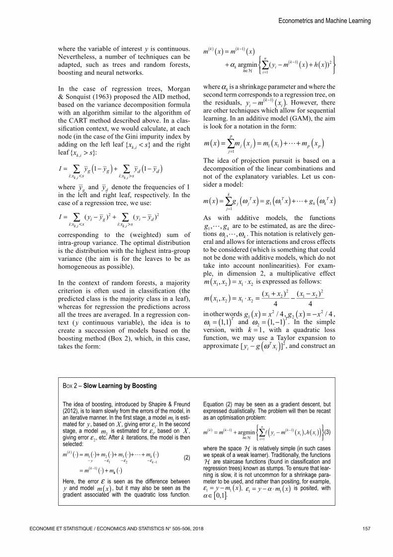
The decision trees thus described are simple to obtain and easy to interpret (as shown by Diagram 3 on the data of the Titanic4), although they are not robust, and their predictive power is often very limited, particularly if the tree is very deep. One obvious idea is to develop a set of more or less independent tree mod‑els which, together, predict better than a sin‑gle‑tree model. The bootstrap method will be used, by sampling (with replacement) n obser‑vations among x yi i,( ){ }. Each sample thus generated can be used to estimate a new classi‑fication tree, thus forming a forest of trees. It is the aggregation of all these trees that gives the prediction. The overall result is less sensitive than the initial sample and often gives better prediction results. These techniques, known as bagging (short for bootstrap aggregating), are similar to bootstrap techniques in regression (for example to construct confidence tubes in a functional regression).4

4. This dataset, which contains information on all the passengers and crew members on the Titanic, with the variable indicating whether the per‑son survived, has been widely used to illustrate classification techniques, see https://www.kaggle.com/c/titanic/data.

Diagram 3Illustration of a Decision Tree Used to Predict the Survival Rate of a Passenger on the Titanic

man? yes no

age > 9.5?

death survival

yes no

yes no

survival

death sibsp > 2.5?

Reading note: A woman (man: no) had a 73% chance of survival, with women representing 36% of the population.

https://www.kaggle.com/c/titanic/data


Bagging involves generating random samples by sampling with replacement from the origi‑nal sample, as with the bootstrap method. Random forests are based on the same princi‑ple as bagging, but during the construction of a classification tree, at each branch, a subset of m covariates is drawn randomly. In other words, each branch of a tree is not based on the same set of covariates. This helps to increase the variability between the trees and, ultimately, to obtain a forest composed of less correlated trees.

Choice of Classification Model

Given a model m ⋅( ) approximating [ | ]Y X x= , and a threshold s ∈[ ]0 1, , let us posit:

y m x sm x sm x s

s

( )[ ]= ( ) > =

( ) >( ) ≤

1

10� si �� si �

The confusion matrix is then the contingency table associated with the countings N Nu v= , with:

N y u y vu vs

n

i

s

j,( )

,( )

=

= = =( )∑1

1

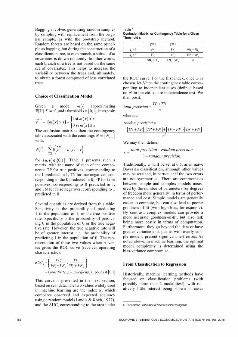
for u v, ,( )∈{ }0 1 . Table 1 presents such a matrix, with the name of each of the compo‑nents: TP for true positives, corresponding to the 1 predicted in 1, TN for true negatives, cor‑responding to the 0 predicted in 0, FP for false positives, corresponding to 0 predicted in 1, and FN for false negatives, corresponding to 1 predicted in 0.

Several quantities are derived from this table. Sensitivity is the probability of predicting 1 in the population of 1, or the true positive rate. Specificity is the probability of predict‑ing 0 in the population of 0 or the true nega‑tive rate. However, the true negative rate will be of greater interest, i.e. the probability of predicting 1 in the population of 0. The rep‑resentation of these two values when s var‑ies gives the ROC curve (receiver operating characteristic):

ROC FPFP VN

VPVP FNs

s

s s

s

s s

s

=+ +

= −

,

,sensitivity specificit1 yys s( ) ∈[ ]pour 0 1,

This curve is presented in the next section, based on real data. The two values widely used in machine learning are the index κ , which compares observed and expected accuracy using a random model (Landis & Koch, 1977), and the AUC, corresponding to the area under

the ROC curve. For the first index, once s is chosen, let N ⊥ be the contingency table corres‑ponding to independent cases (defined based on N in the chi‑square independence test. We then posit:

total precision TP TNn

� = +

whereas:

random precisionTN FP TP FN TP FP TN FN

n

� =+[ ]⋅ +[ ]+ +[ ]⋅ +[ ]

2

We may then define:

κ = −−

total precision random precisionrandom precision

� ��1

Traditionally, s will be set at 0.5, as in naive Bayesian classification, although other values may be retained, in particular if the two errors are not symmetrical. There are compromises between simple and complex models meas‑ured by the number of parameters (or degrees of freedom more generally) in terms of perfor‑mance and cost. Simple models are generally easier to compute, but can also lead to poorer goodness‑of‑fit (with high bias, for example). By contrast, complex models can provide a more accurate goodness‑of‑fit, but also risk being more costly in terms of computation. Furthermore, they go beyond the data or have greater variance and, just as with overly sim‑ple models, present significant test errors. As noted above, in machine learning, the optimal model complexity is determined using the bias‑variance compromise.

From Classification to Regression

Historically, machine learning methods have focused on classification problems (with possibly more than 2 modalities5), with rel‑atively little interest being shown in cases

5. For example, in the case of letter or number recognition.

Table 1Confusion Matrix, or Contingency Table for a Given Threshold s

y = 0 y = 1

ŷs = 0 VNs FNs VNs + FNs

ŷs = 1 FPs VPs FPs + VPs

VNs + FPs FNs + VPs n



where the variable of interest y is continuous. Nevertheless, a number of techniques can be adapted, such as trees and random forests, boosting and neural networks.

In the case of regression trees, Morgan & Sonquist (1963) proposed the AID method, based on the variance decomposition formula with an algorithm similar to the algorithm of the CART method described above. In a clas‑sification context, we would calculate, at each node (in the case of the Gini impurity index by adding on the left leaf { },x sk i < and the right leaf { },x sk i > :

I y y y yi x s

g gi x s

d dk i k i

= −( ) + −( )< >

∑ ∑: :, ,

1 1

where yg and yd denote the frequencies of 1 in the left and right leaf, respectively. In the case of a regression tree, we use:

I y y y yi x s

ii x sk i k i

g i d= − + −< >

∑ ∑: :, ,

( ) ( )2 2

corresponding to the (weighted) sum of intra‑group variance. The optimal distribution is the distribution with the highest intra‑group variance (the aim is for the leaves to be as homogeneous as possible).

In the context of random forests, a majority criterion is often used in classification (the predicted class is the majority class in a leaf), whereas for regression the predictions across all the trees are averaged. In a regression con‑text (y continuous variable), the idea is to create a succession of models based on the boosting method (Box 2), which, in this case, takes the form:

m x m x

y m x h x

k k

ki

n

ik

h

( ) −( )

=

−( )

( ) = ( )+ − ( ) + ( )

∈

∑

1

1

1 2α argmin

( )

where αk is a shrinkage parameter and where the second term corresponds to a regression tree, on the residuals, y m xi

ki− ( )−( )1 . However, there

are other techniques which allow for sequential learning. In an additive model (GAM), the aim is look for a notation in the form:

m x m x m x m xj

p

j j p p( ) = ( ) = ( ) + + ( )=

∑1

1 1

The idea of projection pursuit is based on a decomposition of the linear combinations and not of the explanatory variables. Let us con‑sider a model:

m x g x g x g xj

k

j jT T

k kT( ) = ( ) = ( ) + + ( )

=∑

11 1ω ω ω

As with additive models, the functions g gk1, ,

are to be estimated, as are the direc‑tions ω ω1, , k . This notation is relatively gen‑eral and allows for interactions and cross effects to be considered (which is something that could not be done with additive models, which do not take into account nonlinearities). For exam‑ple, in dimension 2, a multiplicative effect m x x x x1 2 1 2,( ) = ⋅ is expressed as follows:

m x x x x x x x x1 2 1 2

1 22

1 22

4 4, ( ) ( )( ) = ⋅ = + − −

in other words g x x12 4( ) = / , g x x2

2 4( ) = − / , ω1 1 1= ( ), T and ω2 1 1= −( ), T. In the simple version, with k = 1, with a quadratic loss function, we may use a Taylor expansion to approximate [ ]y g xi

Ti− ( )ω 2, and construct an

Box 2 – Slow Learning by Boosting

The idea of boosting, introduced by Shapire & Freund (2012), is to learn slowly from the errors of the model, in an iterative manner. In the first stage, a model m1 is esti‑mated for y, based on X , giving error ε1. In the second stage, a model m2 is estimated for ε1, based on X , giving error ε2, etc. After k iterations, the model is then selected:m m m m m

m m

kkk

k

y

( )

−

−( )

⋅( ) = ⋅( )+ ⋅( )+ ⋅( )+ + ⋅( )

= ⋅( ) +

∼ ∼ ∼ ∼1 2

13

2 1

1

ε ε ε

kk ⋅( )

(2)

Here, the error ε is seen as the difference between y and model m x( ) , but it may also be seen as the gradient associated with the quadratic loss function.

Equation (2) may be seen as a gradient descent, but expressed dualistically. The problem will then be recast as an optimisation problem:

m m y m x h xk k

i

n

ik

i ih

( ) −( )

=

−( )= + − ( ) ( )( )

∈

∑1

1

1argmin

, (3)

where the space is relatively simple (in such cases we speak of a weak learner). Traditionally, the functions are staircase functions (found in classification and regression trees) known as stumps. To ensure that lear‑ning is slow, it is not uncommon for a shrinkage para‑meter to be used, and rather than positing, for example, ε1 1= − ( )y m x , ε α1 1= − ⋅ ( )y m x is posited, with α ∈[ ]0 1, .


iterative algorithm in the standard way. If we have an initial value ω0 , let us note that:

i

n

iT

ii

nT

i

Ti

iT

i

Ti

y g x g x

xy g x

g x

= =∑ ∑− ( ) ≈

+− ( )

(

1

2

10

2

0

0

[ ] '( )

'

ω ω

ωω

ω )) −

ωTix

2

corresponding to approximation in the general‑ised linear models on the function g ⋅( ) which was the link function (assumed to be known). We recognise a weighted least squares prob‑lem. The difficulty here is that the functions g j ⋅( ) are unknown.

Applications

Big Data have required the development of estimation techniques capable of overcoming the limitations of parametric models, which are seen as too restrictive, and of traditional nonparametric models, whose estimation can be difficult in the presence of a large number of variables. Statistical learning, or machine learning, provides new nonparametric estima‑tion methods, which perform well in a general context and in the presence of a large num‑ber of variables.6 However, greater flexibility comes at the cost of a sometimes significant lack of interpretation.

In practice, one important issue is to determine the best model. The answer to this question depends on the underlying problem. If the rela‑tionship between the variables is approximated by a linear model, a correctly specified para‑metric model should perform well. By contrast, if the parametric model is not correctly speci‑fied, since the relationship is highly nonlinear and/or involves significant cross effects, then the statistical methods derived from machine learning should perform better.

The correct specification of a regression model is a common hypothesis, but one that is seldom verified and justified. In the following applica‑tions, we show how statistical methods derived from machine learning can be used to justify the correct specification of a parametric regres‑sion model or to detect a misspecification.

Sales of Child Car Seats (Classification)

Here, we will be drawing on an example used in James et al. (2013). The dataset contains the

sales of child car seats at 400 stores (sales), as well as several variables, including the qua‑lity of the shelving location (shelveloc, equal to “poor”, “average” and “good”) and price (price).67 A binary dependent variable is arti‑ficially created to describe high or low sales (high = “yes” if sales > 8 and “no” if not). In this application, the aim is to identify the deter‑minants of a good volume of sales. We begin by considering a latent linear regression model:

y x GT = + + ∼ ( )γ β ε ε, , ,0 1 (4)

where x is composed of k explanatory varia‑bles, β is a vector of k unknown parameters and ε is an i.i.d. error term with a distribu‑tion function G with zero expectation and unit variance. The dependent variable y∗ is not observed, with only y, with:

yyy

=>≤

10

si �si �

ξξ

(5)

The probability of y being equal to 1 may then be expressed as follows:

Y G xT=( ) = +( )1 0β β (6)

where β γ ξ0 = − .8 This model is estimated by maximum likelihood by selecting a parametric distribution G. If it is assumed that G is the normal distribution, it is a probit model; if it is assumed that G is the logistic distribution, it is a logit model. In a logit/probit model, there are two possible sources of misspecification:

- The linear relationship β β0 + xT is misspec‑ified;

- The parametric distribution used G is incorrect.

In the event of misspecification, of whatever kind, the estimation is no longer valid. The most flexible model is the following:

Y X x G h x= =[ ] = ( )( )1| (7)

where h is an unknown function and G an unknown distribution function. The bagging, random forest and boosting methods can be

6. See, among others, Hastie et al. (2009) and James et al. (2013).7. It is the Carseats dataset from the ISLR library.8. [ ]Y Y x xT T= =] [ > =] [ + + > =] [ > − −1 ξ γ β ε ξ ε ξ γ β which can ultimately be written as [ ]ε γ ξ β< − + xT . Given γ ξ β− = 0, we obtain Y G xT=[ ] = +1 0( )β β . In general, it is assumed that the variance of the error term is equal to σ 2, in which case the parameters of model (6) are β σ0 / and β σ/ , which means that the parameters of latent model (4) are not identifiable and are estimated to within one scale parameter.



used to estimate this general model without making a preliminary choice about the func‑tion h and the distribution G. The estimation of the logit/probit model nevertheless performs better if h and G are correctly specified.

Model (6) is estimated using the logistic dis‑tribution for G, while model (7) is estimated with the bagging, random forest and boosting methods. A 10‑fold cross‑validation analysis is performed (Box 3). The individual probabili‑ties of the out‑of‑sample data, i.e. of each of the folds not used for the estimation, are used to assess the quality of the classification.

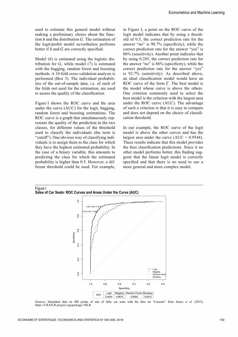
Figure I shows the ROC curve and the area under the curve (AUC) for the logit, bagging, random forest and boosting estimations. The ROC curve is a graph that simultaneously rep‑resents the quality of the prediction in the two classes, for different values of the threshold used to classify the individuals (the term is “cutoff”). One obvious way of classifying indi‑viduals is to assign them to the class for which they have the highest estimated probability. In the case of a binary variable, this amounts to predicting the class for which the estimated probability is higher than 0.5. However, a dif‑ferent threshold could be used. For example,

in Figure I, a point on the ROC curve of the logit model indicates that by using a thresh‑old of 0.5, the correct prediction rate for the answer “no” is 90.7% (specificity), while the correct prediction rate for the answer “yes” is 86% (sensitivity). Another point indicates that by using 0.285, the correct prediction rate for the answer “no” is 86% (specificity), while the correct prediction rate for the answer “yes” is 92.7% (sensitivity). As described above, an ideal classification model would have an ROC curve of the form Γ. The best model is the model whose curve is above the others. One criterion commonly used to select the best model is the criterion with the largest area under the ROC curve (AUC). The advantage of such a criterion is that it is easy to compare and does not depend on the choice of classifi‑cation threshold.

In our example, the ROC curve of the logit model is above the other curves and has the largest area under the curve (AUC = 0.9544). These results indicate that this model provides the best classification predictions. Since it no other model performs better, this finding sug‑gests that the linear logit model is correctly specified and that there is no need to use a more general and more complex model.

Figure ISales of Car Seats: ROC Curves and Areas Under the Curve (AUC)

AUCLogit

0.9544 0.8973 0.9050 0.9313

Specificity

Sen

sitiv

ity

1.0 0.8 0.6 0.4 0.2 0.0

0.0

0.2

0.4

0.6

0.8

1.0

�

�

0.285 (0.860, 0.927)

0.500 (0.907, 0.860)

LogitBaggingRandom forestBoosting

Bagging Random Forest Boosting

Sources: Simulated data on 400 points of sale of baby car seats with the data set “Carseats” from James et al. (2013), https://CRAN.R‑project.org/package=ISLR

https://CRAN.R-project.org/package=ISLR


Purchase of Caravan Insurance (Classification)

Here, we will be drawing on an example used in James et al. (2013). The dataset contains 85 variables on the demographic characteristics of 5,822 individuals.9 The dependent variable (purchase) indicates whether the individual has purchased caravan insurance; it is a binary variable, corresponding to “yes” or “no”. In the dataset, only 6% of the individuals took out such insurance. The classes are therefore highly imbalanced.

Model (6) is estimated using the logistic distri‑bution function, while model (7) is estimated by the bagging, random forest and boosting methods (the tuning parameters are those used by James et al. (2013), n.trees = 1,000 and shrinkage = 0.01). A 10‑fold cross‑validation analysis is performed. The individual probabil‑ities of the out‑of‑sample data, i.e. of each of the pieces not used for the estimation, are used to assess the quality of the classification.

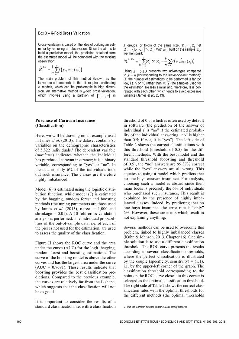
Figure II shows the ROC curve and the area under the curve (AUC) for the logit, bagging, random forest and boosting estimations. The curve of the boosting model is above the other curves and has the largest area under the curve (AUC = 0.7691). These results indicate that boosting provides the best classification pre‑dictions. Compared to the previous example, the curves are relatively far from the L shape, which suggests that the classification will not be as good.

It is important to consider the results of a standard classification, i.e. with a classification

threshold of 0.5, which is often used by default in software (the prediction of the answer of individual i is “no” if the estimated probabi‑lity of the individual answering “no” is higher than 0.5; if not, it is “yes”). The left side of Table 2 shows the correct classifications with this threshold (threshold of 0.5) for the dif‑ferent methods. With the best model and the standard threshold (boosting and threshold of 0.5), the “no” answers are 99.87% correct while the “yes” answers are all wrong. This equates to using a model which predicts that no one buys caravan insurance. For analysts, choosing such a model is absurd since their main focus is precisely the 6% of individuals who purchased such insurance. This result is explained by the presence of highly imba‑lanced classes. Indeed, by predicting that no one buys insurance, the error rate is “only” 6%. However, these are errors which result in not explaining anything.9

Several methods can be used to overcome this problem, linked to highly imbalanced classes (Kuhn & Johnson, 2013, Chapter 16). One sim‑ple solution is to use a different classification threshold. The ROC curve presents the results according to several classification thresholds, where the perfect classification is illustrated by the couple (specificity, sensitivity) = (1,1), i.e. by the upper‑left corner of the graph. The classification threshold corresponding to the point on the ROC curve closest to this corner is selected as the optimal classification threshold. The right side of Table 2 shows the correct clas‑sification rates with the optimal thresholds for the different methods (the optimal thresholds

9. It is the Caravan dataset from the ISLR library under R.

Box 3 – K‑Fold Cross Validation

Cross‑validation is based on the idea of building an esti‑mator by removing an observation. Since the aim is to build a predictive model, the prediction obtained from the estimated model will be compared with the missing observation:

� CV= ( )( )

=∑1

1ny m x

i

n

i i i, ( )

The main problem of this method (known as the leave‑one‑out method) is that it requires calibrating n models, which can be problematic in high dimen‑sion. An alternative method is k‑fold cross‑validation, which involves using a partition of 1, , n{ } in

k groups (or folds) of the same size, 1, , k (let j jn= { }1, , ). With m j

( ) built on the sample j , we then posit:

k

j

k

jk−

=

= ∑� CV 1

1

or

ji

i j ikn

y m xj

= ( )( )∈

( )∑ ,

Using k = 5 10, presents two advantages compared to k n= (corresponding to the leave‑one‑out method): (1) the number of estimations to be performed is far too low, i.e. 5 or 10 rather than n; (2) the samples used for the estimation are less similar and, therefore, less cor‑related with each other, which tends to avoid excessive variance (James et al., 2013).



of the logit, bagging, random forest and boost‑ing methods are 0.0655, 0.0365, 0.0395 and 0.0596, respectively). With boosting and an optimal threshold, the “no” answers are 68.6% correct, while the “yes” answers are 73.85% correct. The aim of the analysis being to cor‑rectly predict the individuals likely to buy cara‑van insurance (“yes” class) and to distinguish them sufficiently from the others (“no” class), the optimal threshold performs far better than the standard threshold (0.5). With a logit model and an optimal threshold, the correct classifica‑tion rate for the “no” class is 72.78%, while the rate for the “yes” class is 63.51%. Compared to boosting, the logit model is slightly better at

predicting the “no” class, but is significantly worse at predicting the “yes” class.

Personal Loan Defaults (Classification)

Consider the German database of per‑sonal loans, used in Nisbet et al. (2001) and Tuffery (2001), with 1,000 observations and 19 explanatory variables, including 12 quali‑tative variables: by disjuncting them (by cre‑ating an indicator variable for each modality), we obtain 48 potential explanatory variables. A recurring question in modelling is to deter‑mine which variables merit being used. The

Figure IIPurchase of Insurance: ROC Curves and Areas Under the Curve (AUC)

Specificity

Sen

sitiv

ity

1.0 0.8 0.6 0.4 0.2 0.0

0.0

0.2

0.4

0.6

0.8

1.0

LogitBaggingRandom forestBoosting

AUC0.7372 0.7198 0.7154 0.7691

Logit Bagging Random Forest Boosting

Sources: Experimental dataset “Caravan” on the consumption of caravan insurance, James et al. (2013). https://CRAN.R‑project.org/package=ISLR

Table 2Purchase of Insurance: Sensitivity to the Choice of Classification Threshold

Threshold of 0.5 Optimal Thresholds

Specificity Sensitivity Specificity Sensitivity

Logit 0.9967 0.0057 0.7278 0.6351

Bagging 0.9779 0.0661 0.6443 0.7069

Random Forest 0.9892 0.0316 0.6345 0.6954

Boosting 0.9987 0.0000 0.6860 0.7385Sources: Experimental dataset “Caravan” on the consumption of caravan insurance, James et al. (2013). https://CRAN.R‑project.org/package=ISLR




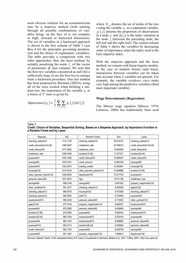
most obvious solution for an econometrician may be a stepwise method (with running through all possible combinations of vari‑ables being, on the face of it, too complex in high, forward or backward dimension). The set of variables in a backward approach is shown in the first column of Table 3 (see Box 4 for the principles governing penalisa‑tion and the choice of explanatory variables). The table provides a comparison with two other approaches: first, the lasso method, by suitably penalising the norm

1 of the vector of parameters β (last column). We note that the first two variables considered as null (for a sufficiently large λ) are the first two to emerge from a backward procedure. One last method has been proposed by Breiman (2001b), using all of the trees created when building a ran‑dom tree: the importance of the variable xk in a forest of T trees is given by:

Importance xT

p j jkt

n

j Nt

t k

( ) = ( ) ( )= ∈∑ ∑1

1 ,

∆

where Nt k, denotes the set of nodes of the tree t using the variable xk as a separation variable, p jt ( ) denotes the proportion of observations in a node j, and ∆ j( ) is the index variation at the node j (between the preceding node, the left leaf and the right leaf). The central column of Table 3 shows the variables by decreasing order of importance when the index used is the Gini impurity index.

With the stepwise approach and the lasso method, we remain with linear logistic models. In the case of random forests (and trees), interactions between variables can be taken into account when 2 variables are present. For example, the variable residence_since ranks very high among the predictive variables (third most important variable).

Wage Determinants (Regression)

The Mincer wage equation (Mincer, 1974; Lemieux, 2006) has traditionally been used

Table 3Credit: Choice of Variables, Sequential Sorting, Based on a Stepwise Approach, by Importance Function in a Random Forest and by Lasso

Stepwise AIC Random Forest Gini Lassochecking_statusA14 1112.1730 checking_statusA14 30.818197 checking_statusA14credit_amount(4e+03,Inf] 1090.3467 installment_rate 20.786313 credit_amount(4e+03,Inf]credit_historyA34 1071.8062 residence_since 19.853029 credit_historyA34installment_rate 1056.3428 duration(15,36] 11.377471 duration(36,Inf]purposeA41 1044.1580 credit_historyA34 10.966407 credit_historyA31savingsA65 1033.7521 credit_amount 10.964186 savingsA65purposeA43 1023.4673 existing_credits 10.482961 housingA152housingA152 1015.3619 other_payment_plansA143 10.469886 duration(15,36]other_payment_plansA143 1008.8532 telephoneA192 10.217750 purposeA41personal_statusA93 1001.6574 Age 10.071736 installment_ratesavingsA64 996.0108 savingsA65 9.547362 property_magnitudeA124other_partiesA103 991.0377 checking_statusA12 9.502445 age(25,Inf]checking_statusA13 985.9720 housingA152 8.757095 checking_statusA13checking_statusA12 982.9530 jobA173 8.734460 purposeA43employmentA74 980.2228 personal_statusA93 8.715932 other_partiesA103age(25,Inf] 977.9145 property_magnitudeA123 8.634527 employmentA72purposeA42 975.2365 personal_statusA92 8.438480 savingsA64duration(15,36] 972.5094 purposeA43 8.362432 employmentA74duration(36,Inf] 966.7004 employmentA73 8.225416 purposeA46purposeA49 965.1470 employmentA75 8.089682 personal_statusA93purposeA410 963.2713 duration(36,Inf] 8.029945 personal_statusA92credit_historyA31 962.1370 purposeA42 8.025749 savingsA63

purposeA48 961.1567 property_magnitudeA122 7.908813 telephoneA192Sources: Dataset “Credit” of the casdataset library of R, loans to households in Germany (Nisbet et al., 2001; Tufféry, 2001). http://cas.uqam.ca/



to explain (individual) wages according to the individual’s education, experience and gender:

log wage( ) =+ + + + +β β β β β ε0 1 2 3

24ed feexp exp (9)

where ed is the level of education, exp is the level of professional experience and fe is a dummy variable equal to 1 if the individual is a woman. According to human capital theory, the expected wage increases with experience, at an increasingly slow rate, until it reaches a threshold before decreasing. The introduction of the square of exp enables such a relationship to be taken into account. The presence of var‑iable fe allows for any wage gap between men and women to be measured.

Model (9) establishes a linear relationship between wage and level of education and a quadratic relationship between wage and pro‑fessional experience. These relationships may seem too restrictive. Several studies have shown, in particular, that wages do not fall after a certain age and that a quadratic rela‑tionship or a higher‑degree polynomial is more appropriate (Murphy & Welch, 1990; Bazen & Charni, 2017).

Model (9) also establishes that the wage gap between men and women is independent of the level of education and experience. It is too restrictive if, for example, the average wage gap between men and women is low for unskilled jobs and high for skilled jobs, or low among early‑career workers and high among late career workers (interaction effects). The most flexible model is the fully nonparametric model:

log wage exp( ) = ( ) +m ed fe,� ,� ε (10)

where m ⋅( ) is a random function. It has the advantage of being able to take into account any nonlinear relationships and complex inter‑actions between the variables. However, its significant flexibility is at the cost of a more difficult interpretation of the model. Indeed, a 4‑dimensional graph would be needed to rep‑resent the function m. One solution is to repre‑sent the function m in 3 dimensions by fixing the value of one of the variables, although the represented function may differ significantly with a different fixed value.

We will use data from a survey by the US Census Bureau carried out in May 1985 drawn from Berndt (1990) and available under R.10 The two models are estimated and a 10‑fold cross‑ validation analysis is used to select the best approach. Parametric model (9) is estimated by ordinary least squares (OLS). Fully nonpara‑metric model (10) is estimated by the method of splines since it includes few variables and also by the bagging, random forest and boosting methods.

The results of the 10‑fold cross‑validation are presented in Table 4. The best model is the model that minimises the criterion

10− � CV. The results show that model (9) is at least as effec‑tive as model (10), which suggests that para‑metric model (9) is correctly specified.

Determinants of House Prices in Boston (Regression)

Here, we will be drawing on one of the exam‑ples used in James et al. (2013), whose data

10. It is the CPS1985 dataset from the AER library.

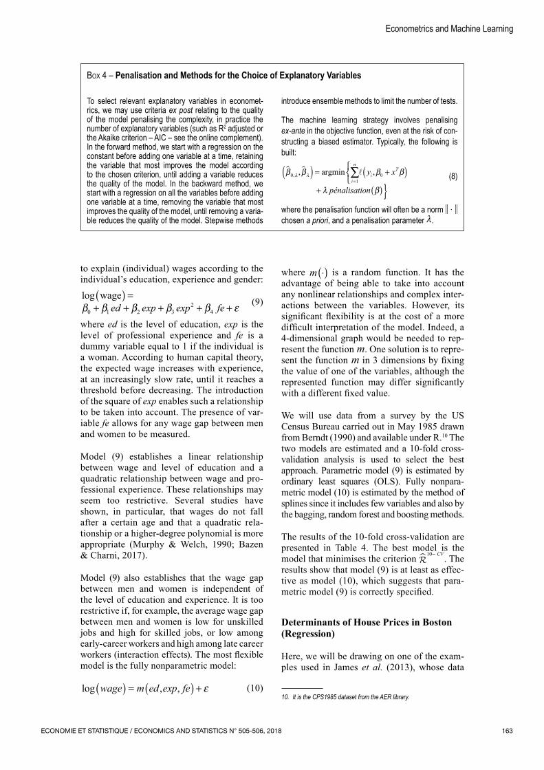
Box 4 – Penalisation and Methods for the Choice of Explanatory Variables

To select relevant explanatory variables in economet‑rics, we may use criteria ex post relating to the quality of the model penalising the complexity, in practice the number of explanatory variables (such as R2 adjusted or the Akaike criterion – AIC – see the online complement). In the forward method, we start with a regression on the constant before adding one variable at a time, retaining the variable that most improves the model according to the chosen criterion, until adding a variable reduces the quality of the model. In the backward method, we start with a regression on all the variables before adding one variable at a time, removing the variable that most improves the quality of the model, until removing a varia‑ble reduces the quality of the model. Stepwise methods

introduce ensemble methods to limit the number of tests.

The machine learning strategy involves penalising ex‑ante in the objective function, even at the risk of con‑structing a biased estimator. Typically, the following is built:

β β β β

λ β

λ λ

01

0, , ,

�

( ) = +( )

+ ( )}=∑argmini

n

iTy x

pénalisation

(8)

where the penalisation function will often be a norm ⋅ chosen a priori, and a penalisation parameter λ.


are available under R. The dataset contains the median values of house prices (medv) in n = 506 neighbourhoods around Boston along with 13 other variables, including the average number of rooms per house (rm), the ave‑rage age of houses (age) and the percentage of households with a low economic status (lstat).11

Consider the following linear regression model:

medv xT= + +α β ε (11)

where x = [chas,nox,age,tax,indus,rad,dis,lstat, crim,black,rm,zn,ptratio] is a vector in dimen‑sion 13 and β is a vector of 13 parameters. This model specifies a linear relationship between the value of houses and each of the explanatory variables. The most flexible model is the fully nonparametric model:

medv m x= ( ) + ε . (12)

The estimation of this model by the Kernel method or the method of splines can be prob‑lematic since the number of variables is rela‑tively high (there are 13 variables here) or, at least, too high to consider estimating a surface in dimension 13. We estimate the two models and use a 10‑fold cross‑validation analysis to select the best approach. Parametric model (11) is estimated by ordinary least squares

(OLS) and fully nonparametric model (12) is estimated using three different methods: bag‑ging, random forest and boosting (here we use the default values used in James et al., 2013, pp. 328–331).11

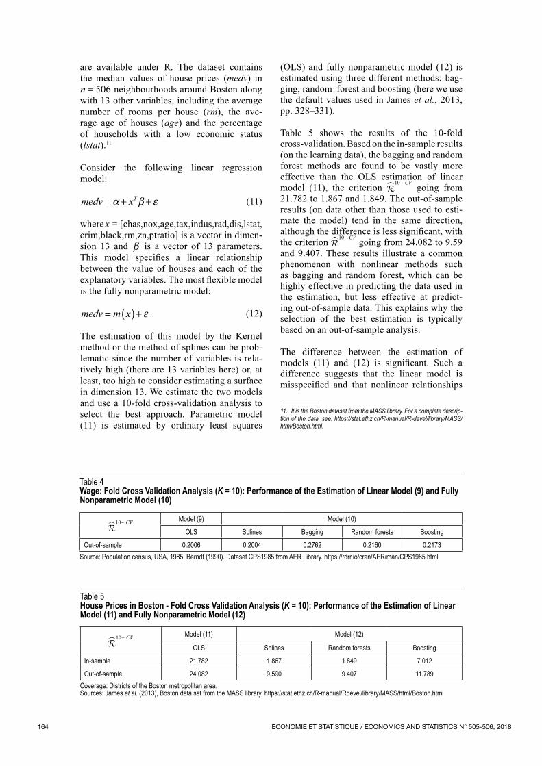
Table 5 shows the results of the 10‑fold cross‑validation. Based on the in‑sample results (on the learning data), the bagging and random forest methods are found to be vastly more effective than the OLS estimation of linear model (11), the criterion

10− � CV going from 21.782 to 1.867 and 1.849. The out‑of‑sample results (on data other than those used to esti‑mate the model) tend in the same direction, although the difference is less significant, with the criterion

10− � CV going from 24.082 to 9.59 and 9.407. These results illustrate a common phenomenon with nonlinear methods such as bagging and random forest, which can be highly effective in predicting the data used in the estimation, but less effective at predict‑ing out‑of‑sample data. This explains why the selection of the best estimation is typically based on an out‑of‑sample analysis.

The difference between the estimation of models (11) and (12) is significant. Such a difference suggests that the linear model is mis specified and that nonlinear relationships

11. It is the Boston dataset from the MASS library. For a complete descrip‑tion of the data, see: https://stat.ethz.ch/R‑manual/R‑devel/library/MASS/html/Boston.html.

Table 5House Prices in Boston ‑ Fold Cross Validation Analysis (K = 10): Performance of the Estimation of Linear Model (11) and Fully Nonparametric Model (12)

10− � CV Model (11) Model (12)

OLS Splines Random forests Boosting

In‑sample 21.782 1.867 1.849 7.012

Out‑of‑sample 24.082 9.590 9.407 11.789Coverage: Districts of the Boston metropolitan area.Sources: James et al. (2013), Boston data set from the MASS library. https://stat.ethz.ch/R‑manual/Rdevel/library/MASS/html/Boston.html

Table 4Wage: Fold Cross Validation Analysis (K = 10): Performance of the Estimation of Linear Model (9) and Fully Nonparametric Model (10)

10− � CV Model (9) Model (10)

OLS Splines Bagging Random forests Boosting

Out‑of‑sample 0.2006 0.2004 0.2762 0.2160 0.2173Source: Population census, USA, 1985, Berndt (1990). Dataset CPS1985 from AER Library. https://rdrr.io/cran/AER/man/CPS1985.html

https://stat.ethz.ch/R-manual/R-devel/library/MASS/html/Boston.html




and/or interaction effects are present in the relationship between house prices and the explanatory variables x. This requires looking for a better parametric specification. Based on parametric model (11), and in order to take into account any potential nonlinearities, the following generalised additive model (GAM) may be considered:

medv m x m x m x= ( ) + ( ) +…+ ( ) +1 1 2 2 13 13 ε (13)

where m m m1 2 13, ,… are unknown functions. The advantage of this model is that it allows for any nonlinear relationship between the dependent variable and each of the explana‑tory variables to be considered. Furthermore, it does not suffer from the curse of dimen‑sionality problem since each of the functions is of dimension 1 and it is easily interpret‑able. However, it does not take into account any potential interaction effects. The estima‑tion of generalised additive model (13) by the method of splines, as part of a 10‑fold cross‑ validation analysis, gives value

1013 643

−=

� CV. .

Compared to parametric model (11), there is a significant gain (13.643 vs. 24.082). However, the difference with the fully nonparametric model (12) remains substantial (13.643 vs 9.590, 9.407, 11.789). Such a difference sug‑gests that taking into account individual rela‑tionships which may be highly nonlinear is not sufficient and that interaction effects between variables are present. The simplest interaction variables among the pairs of variables (x xi j× ) could be included in the model, but that would imply adding a significant number of variables to the original model (78 in this case), which would have an impact on the quality of the estimation of the model. In any case, as things stand, what can be said is that the linear model is misspecified and that there are potentially significant interaction effects in the relation‑ship between medv and X , the identification of such effects remaining a delicate matter.

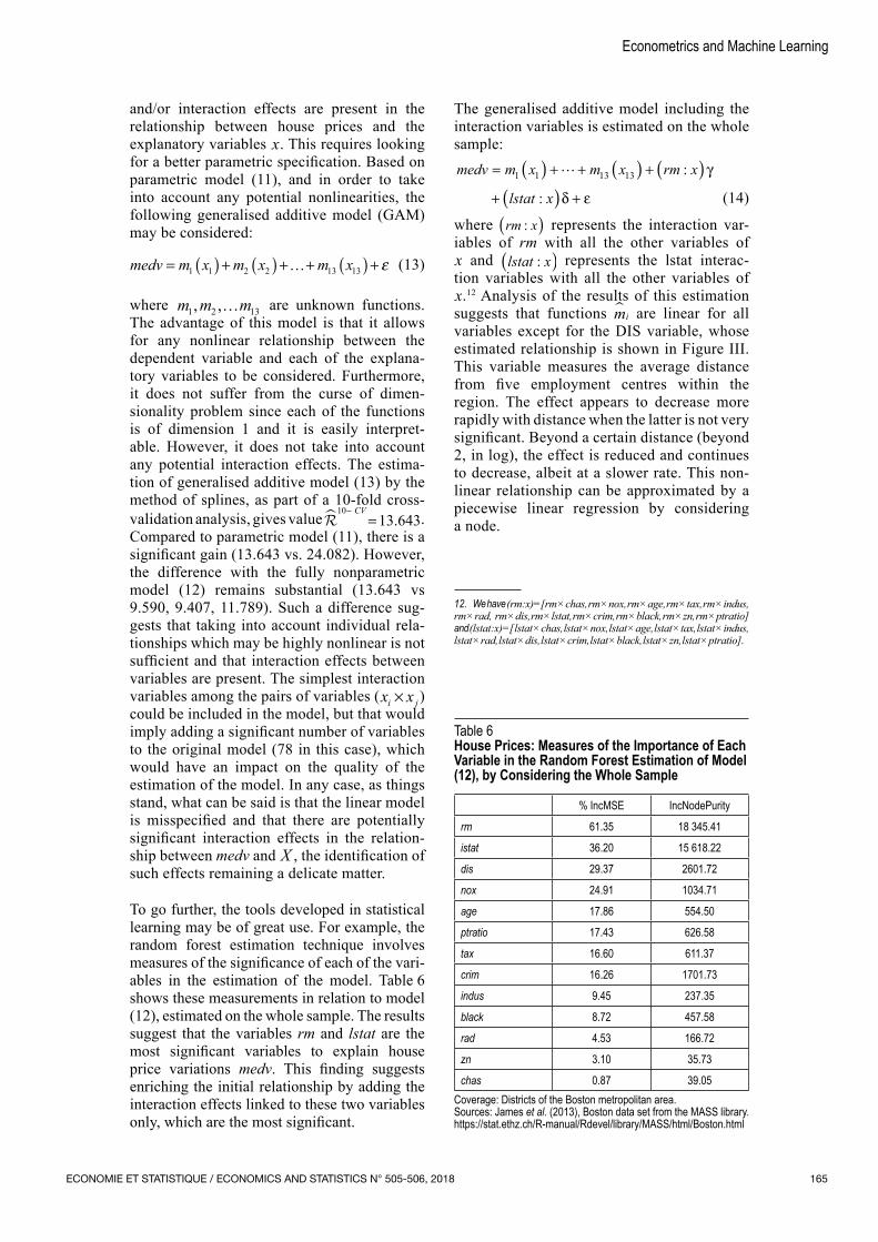
To go further, the tools developed in statistical learning may be of great use. For example, the random forest estimation technique involves measures of the significance of each of the vari‑ables in the estimation of the model. Table 6 shows these measurements in relation to model (12), estimated on the whole sample. The results suggest that the variables rm and lstat are the most significant variables to explain house price variations medv. This finding suggests enriching the initial relationship by adding the interaction effects linked to these two variables only, which are the most significant.

The generalised additive model including the interaction variables is estimated on the whole sample:medv m x m x rm x

lstat x

= + + +

+ +

( ) ( ) ( )( )

1 1 13 13 :

:

γ

δ ε (14)

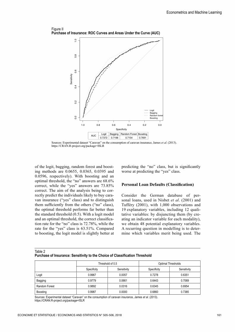
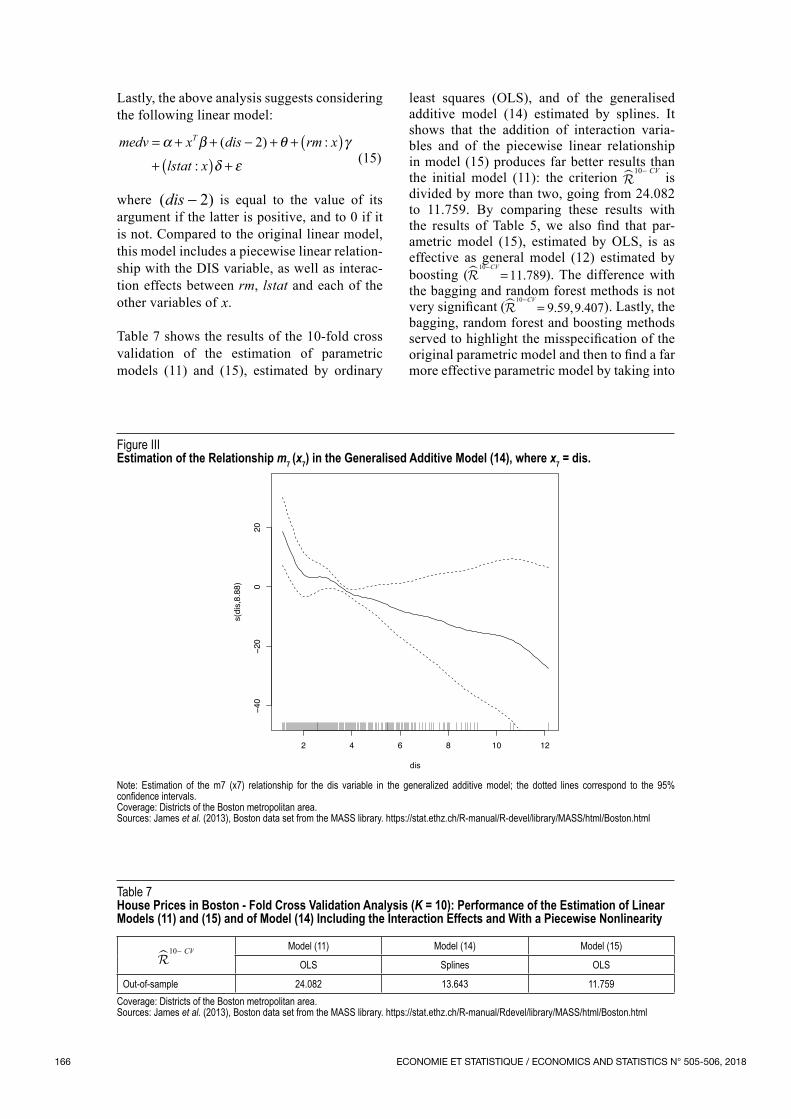
where rm x:( ) represents the interaction var‑iables of rm with all the other variables of x and lstat x:( ) represents the lstat interac‑tion variables with all the other variables of x.12 Analysis of the results of this estimation suggests that functions mi

are linear for all variables except for the DIS variable, whose estimated relationship is shown in Figure III. This variable measures the average distance from five employment centres within the region. The effect appears to decrease more rapidly with distance when the latter is not very significant. Beyond a certain distance (beyond 2, in log), the effect is reduced and continues to decrease, albeit at a slower rate. This non‑linear relationship can be approximated by a piecewise linear regression by considering a node.

12. We have (rm:x)=[rm × chas, rm × nox, rm × age, rm × tax, rm × indus, rm × rad, rm × dis, rm × lstat, rm × crim, rm × black, rm × zn, rm × ptratio] and (lstat:x)=[ lstat × chas, lstat × nox, lstat × age, lstat × tax, lstat × indus, lstat × rad, lstat × dis, lstat × crim, lstat × black, lstat × zn, lstat × ptratio].

Table 6House Prices: Measures of the Importance of Each Variable in the Random Forest Estimation of Model (12), by Considering the Whole Sample

% IncMSE IncNodePurity

rm 61.35 18 345.41

istat 36.20 15 618.22

dis 29.37 2601.72

nox 24.91 1034.71

age 17.86 554.50

ptratio 17.43 626.58

tax 16.60 611.37

crim 16.26 1701.73

indus 9.45 237.35

black 8.72 457.58

rad 4.53 166.72

zn 3.10 35.73

chas 0.87 39.05Coverage: Districts of the Boston metropolitan area.Sources: James et al. (2013), Boston data set from the MASS library. https://stat.ethz.ch/R‑manual/Rdevel/library/MASS/html/Boston.html


Lastly, the above analysis suggests considering the following linear model:

medv x dis rm x

lstat x

T= + + − + + ( )+ ( ) +

α β θ γ

δ ε

( ) :

:

2

(15)

where ( )dis − 2 is equal to the value of its argument if the latter is positive, and to 0 if it is not. Compared to the original linear model, this model includes a piecewise linear relation‑ship with the DIS variable, as well as interac‑tion effects between rm, lstat and each of the other variables of x.

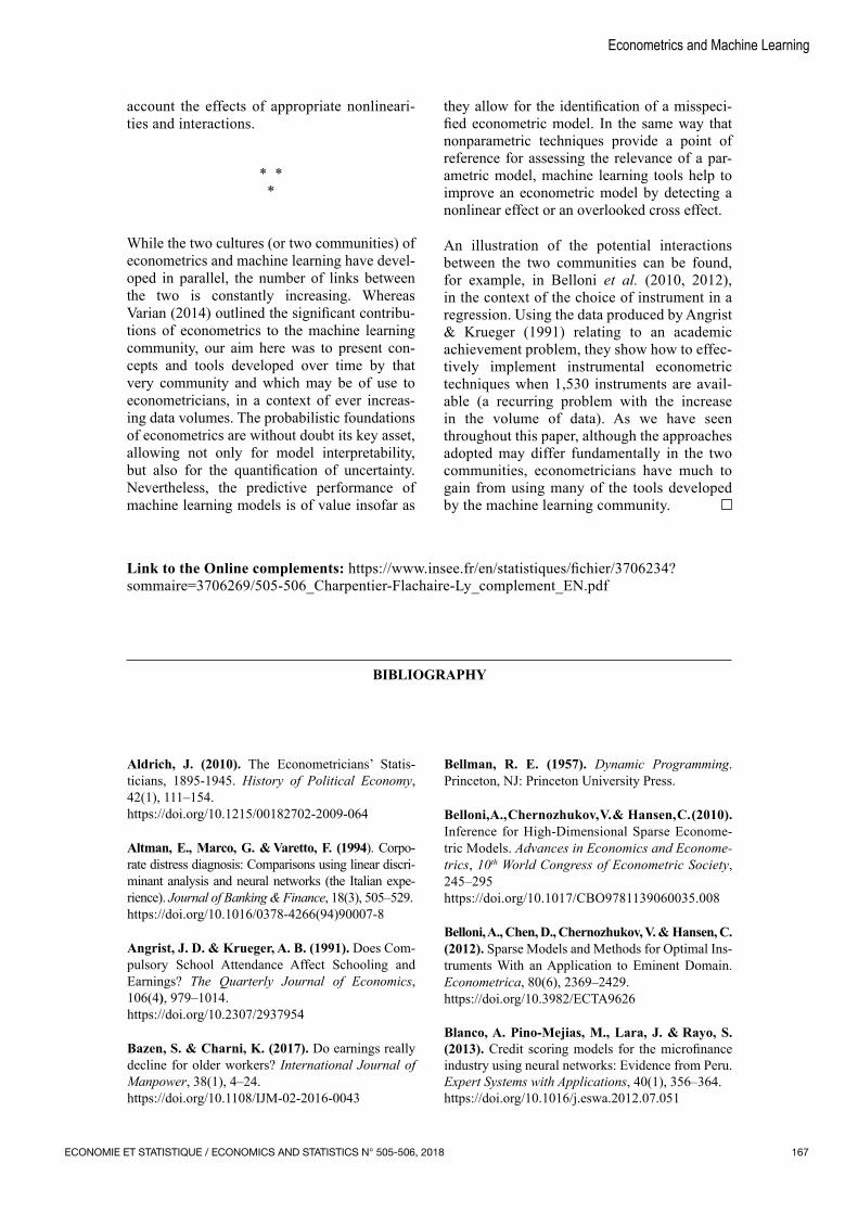
Table 7 shows the results of the 10‑fold cross validation of the estimation of parametric models (11) and (15), estimated by ordinary

least squares (OLS), and of the generalised additive model (14) estimated by splines. It shows that the addition of interaction varia‑bles and of the piecewise linear relationship in model (15) produces far better results than the initial model (11): the criterion

10− � CV is divided by more than two, going from 24.082 to 11.759. By comparing these results with the results of Table 5, we also find that par‑ametric model (15), estimated by OLS, is as effective as general model (12) estimated by boosting (

1011 789

−=

CV. ). The difference with

the bagging and random forest methods is not very significant (

109 59 9 407

−=

CV. , . ). Lastly, the

bagging, random forest and boosting methods served to highlight the misspecification of the original parametric model and then to find a far more effective parametric model by taking into

Table 7House Prices in Boston ‑ Fold Cross Validation Analysis (K = 10): Performance of the Estimation of Linear Models (11) and (15) and of Model (14) Including the Interaction Effects and With a Piecewise Nonlinearity

10− � CV Model (11) Model (14) Model (15)

OLS Splines OLS

Out‑of‑sample 24.082 13.643 11.759Coverage: Districts of the Boston metropolitan area.Sources: James et al. (2013), Boston data set from the MASS library. https://stat.ethz.ch/R‑manual/Rdevel/library/MASS/html/Boston.html

Figure IIIEstimation of the Relationship m7 (x7) in the Generalised Additive Model (14), where x7 = dis.

2 4 6 8 10 12

−40

−20

020

dis

s(dis,8.88)

Note: Estimation of the m7 (x7) relationship for the dis variable in the generalized additive model; the dotted lines correspond to the 95% confidence intervals.Coverage: Districts of the Boston metropolitan area.Sources: James et al. (2013), Boston data set from the MASS library. https://stat.ethz.ch/R‑manual/R‑devel/library/MASS/html/Boston.html




account the effects of appropriate nonlineari‑ties and interactions.

* * *

While the two cultures (or two communities) of econometrics and machine learning have devel‑oped in parallel, the number of links between the two is constantly increasing. Whereas Varian (2014) outlined the significant contribu‑tions of econometrics to the machine learning community, our aim here was to present con‑cepts and tools developed over time by that very community and which may be of use to econometricians, in a context of ever increas‑ing data volumes. The probabilistic foundations of econometrics are without doubt its key asset, allowing not only for model interpretability, but also for the quantification of uncertainty. Nevertheless, the predictive performance of machine learning models is of value insofar as

they allow for the identification of a misspeci‑fied econometric model. In the same way that nonparametric techniques provide a point of reference for assessing the relevance of a par‑ametric model, machine learning tools help to improve an econometric model by detecting a nonlinear effect or an overlooked cross effect.

An illustration of the potential interactions between the two communities can be found, for example, in Belloni et al. (2010, 2012), in the context of the choice of instrument in a regression. Using the data produced by Angrist & Krueger (1991) relating to an academic achievement problem, they show how to effec‑tively implement instrumental econometric techniques when 1,530 instruments are avail‑able (a recurring problem with the increase in the volume of data). As we have seen throughout this paper, although the approaches adopted may differ fundamentally in the two communities, econometricians have much to gain from using many of the tools developed by the machine learning community.

Aldrich, J. (2010). The Econometricians’ Statis‑ticians, 1895‑1945. History of Political Economy, 42(1), 111–154. https://doi.org/10.1215/00182702‑2009‑064

Altman, E., Marco, G. & Varetto, F. (1994). Corpo‑rate distress diagnosis: Comparisons using linear discri‑minant analysis and neural networks (the Italian expe‑rience). Journal of Banking & Finance, 18(3), 505–529. https://doi.org/10.1016/0378‑4266(94)90007‑8

Angrist, J. D. & Krueger, A. B. (1991). Does Com‑pulsory School Attendance Affect Schooling and Earnings? The Quarterly Journal of Economics, 106(4), 979–1014. https://doi.org/10.2307/2937954

Bazen, S. & Charni, K. (2017). Do earnings really decline for older workers? International Journal of Manpower, 38(1), 4–24.https://doi.org/10.1108/IJM‑02‑2016‑0043

Bellman, R. E. (1957). Dynamic Programming. Princeton, NJ: Princeton University Press.

Belloni, A., Chernozhukov, V. & Hansen, C. (2010). Inference for High‑Dimensional Sparse Econome‑tric Models. Advances in Economics and Econome-trics, 10th World Congress of Econometric Society, 245–295 https://doi.org/10.1017/CBO9781139060035.008

Belloni, A., Chen, D., Chernozhukov, V. & Hansen, C. (2012). Sparse Models and Methods for Optimal Ins‑truments With an Application to Eminent Domain. Econometrica, 80(6), 2369–2429. https://doi.org/10.3982/ECTA9626

Blanco, A. Pino‑Mejias, M., Lara, J. & Rayo, S. (2013). Credit scoring models for the microfinance industry using neural networks: Evidence from Peru. Expert Systems with Applications, 40(1), 356–364. https://doi.org/10.1016/j.eswa.2012.07.051

BIBLIOGRAPHY

Link to the Online complements: https://www.insee.fr/en/statistiques/fichier/3706234? sommaire=3706269/505‑506_Charpentier‑Flachaire‑Ly_complement_EN.pdf

https://doi.org/10.1215/00182702-2009-064

https://doi.org/10.1016/0378-4266(94)90007-8

https://doi.org/10.2307/2937954

https://doi.org/10.1017/CBO9781139060035.008

https://doi.org/10.3982/ECTA9626

https://doi.org/10.1016/j.eswa.2012.07.051


Breiman, L. Fiedman, J., Olshen, R. A. & Stone, C. J. (1984). Classification And Regression Trees. Chapman & Hall/CRC Press Online.https://www.stat.wisc.edu/~loh/treeprogs/guide/wires11.pdf

Breiman, L. (2001a). Statistical Modeling: The Two Cultures. Statistical Science, 16(3), 199–231.https://doi.org/10.1214/ss/1009213726

Breiman, L. (2001b). Random forests. Machine learning, 45(1), 5–32. https://doi.org/10.1023/A:1010933404324

Bühlmann, P. & van de Geer, S. (2011). Statistics for High Dimensional Data: Methods, Theory and Applications. Berlin: Springer Verlag.https://doi.org/10.1007/978‑3‑642‑20192‑9

Cortes, C. & Vapnik, V. (1995). Support‑Vector Networks. Machine Learning, 20(3), 273–297. https://doi.org/10.1023/A:1022627411411

Grandvalet, Y., Mariéthoz, J., & Bengio, S. (2005). Interpretation of SVMs with an Application to Unba‑lanced Classification. Advances in Neural Informa-tion Processing Systems N° 18. https://papers.nips.cc/paper/2763‑a‑probabilistic‑ interpretation‑of‑svms‑with‑an‑application‑to‑ unbalanced‑classification.pdf

Groves, T. & Rothenberg, T. (1969). A note on the expected value of an inverse matrix. Biometrika, 56(3), 690–691. https://doi.org/10.1093/biomet/56.3.690

Hastie, T., Tibshirani, R. & Friedman, J. (2009). The Elements of Statistical Learning. New York: Springer Verlag.https://doi.org/10.1007/978‑0‑387‑84858‑7

Hebb, D. O. (1949). The organization of behavior. New York: Wiley.https://doi.org/10.1002/1097‑4679(195007)6:3<307:: AID‑JCLP2270060338>3.0.CO;2‑K

James, G., D. Witten, T. Hastie, & Tibshirani, R. (2013). An Introduction to Statistical Learning. Springer Texts in Statistics 103. https://doi.org/10.1007/978‑1‑4614‑7138‑7

Khashman, A. (2011). Credit risk evaluation using neural networks: Emotional versus conventional models. Applied Soft Computing, 11(8), 5477–5484. https://doi.org/10.1016/j.asoc.2011.05.011

Kolda, T. G. & Bader, B. W. (2009). Tensor Decom‑positions and Applications. SIAM Review, 51(3), 455–500.https://doi.org/10.1137/07070111X

Kuhn, M. & Johnson, K. (2013). Applied Predic-tive Modeling. New York: Springer Verlag. https://doi.org/10.1007/978‑1‑4614‑6849‑3

Landis, J. R. & Koch, G.G. (1977). The Measure‑ment of Observer Agreement for Categorical Data. Biometrics, 33(1), 159–174.https://doi.org/10.2307/2529310

LeCun, Y., Bengio, Y. & Hinton, G. (2015). Deep learning. Nature, 521, 436–444.https://doi.org/10.1038/nature14539

Leeb, H. (2008). Evaluation and selection of models for out‑of‑sample prediction when the sample size is small relative to the complexity of the data‑ generating process. Bernoulli, 14(3), 661–690. https://doi.org/10.3150/08‑BEJ127

Lemieux, T. (2006). The “Mincer Equation” Thirty Years After Schooling, Experience, and Earnings. In: Grossbard, S. (Ed.), Jacob Mincer: A Pioneer of Modern Labor Economics, pp. 127–145. Boston, MA: Springer Verlag.https://doi.org/10.1007/0‑387‑29175‑X_11

Lin, H. W., Tegmark, M. & Rolnick, D. (2016). Why does deep and cheap learning work so well? https://arxiv.org/abs/1608.08225

Mincer, J. (1974). Schooling, Experience and Ear‑nings. New York: NBER.https://www.nber.org/books/minc74‑1

Morgan, J. N. & Sonquist, J. A. (1963). Problems in the Analysis of Survey Data, and a Proposal. Journal of the American Statistical Association, 58(302), 415–434.https://doi.org/10.1080/01621459.1963.10500855

Morgan, M. S. (1990). The history of econometric ideas. Cambridge, UK: Cambridge University Press.

Murphy, K. M. & Welch, F. (1990). Empirical Age‑Earnings Profiles. Journal of Labor Economics, 8(2), 202–229.https://doi.org/10.1086/298220

Nisbet, R., Elder, J. & Miner, G. (2011). Handbook of Statistical Analysis and Data Mining Applications. New York: Academic Press.

Portnoy, S. (1988). Asymptotic Behavior of Like‑lihood Methods for Exponential Families when the Number of Parameters Tends to Infinity. Annals of Statistics, 16(1), 356–366.https://doi.org/10.1214/aos/1176350710

Quinlan, J. R. (1986). Induction of decision trees. Machine Learning, 1(1), 81–106.https://doi.org/10.1007/BF00116251

https://www.stat.wisc.edu/~loh/treeprogs/guide/wires11.pdf

https://www.stat.wisc.edu/~loh/treeprogs/guide/wires11.pdf

https://doi.org/10.1214/ss/1009213726

https://doi.org/10.1023/A:1010933404324

https://doi.org/10.1007/978-3-642-20192-9

https://doi.org/10.1023/A:1022627411411

https://papers.nips.cc/paper/2763-a-probabilistic-interpretation-of-svms-with-an-application-to-unbalanced-classification.pdf



https://doi.org/10.1093/biomet/56.3.690

https://doi.org/10.1007/978-0-387-84858-7

https://doi.org/10.1002/1097-4679(195007)6:3<307::AID-JCLP2270060338>3.0.CO;2-K

https://doi.org/10.1002/1097-4679(195007)6:3<307::AID-JCLP2270060338>3.0.CO;2-K

https://doi.org/10.1007/978-1-4614-7138-7

https://doi.org/10.1016/j.asoc.2011.05.011

https://doi.org/10.1137/07070111X

https://doi.org/10.1007/978-1-4614-6849-3

https://doi.org/10.2307/2529310

https://doi.org/10.1038/nature14539

https://doi.org/10.3150/08-BEJ127

https://doi.org/10.1007/0-387-29175-X_11

https://arxiv.org/abs/1608.08225

https://www.nber.org/books/minc74-1

https://doi.org/10.1080/01621459.1963.10500855

https://doi.org/10.1086/298220

https://doi.org/10.1214/aos/1176350710

https://doi.org/10.1007/BF00116251



Rosenblatt, F. (1958). The perceptron: A proba‑bilistic model for information storage and organi‑zation in the brain. Psychological Review, 65(6), 386–408.https://doi.org/10.1037/h0042519

Samuel, A. (1959). Some Studies in Machine Lear‑ning Using the Game of Checkers. IBM Journal of Research and Development, 3(3), 210–229. https://doi.org/10.1147/rd.33.0210

Shalev‑Shwartz, S. & Ben‑David, S. (2014). Unders-tanding Machine Learning: From Theory to Algo-rithms. Cambridge, UK: Cambridge University Press.

Shapire, R. E. & Freund, Y. (2012). Boosting. Fon-dations and Algorithms. Cambridge, A MIT Press.

Tam, K. Y. & Kiang, M. Y. (1992). Managerial applications of neural networks: The case of bank failure predictions. Management Science, 38, 926–947.https://doi.org/10.1287/mnsc.38.7.926

Tufféry, S. (2001). Data Mining and Statistics for Decision Making. Hoboken, NJ: Wiley.

Varian, H. R. (2014). Big Data: New Tricks for Econometrics. Journal of Economic Perspectives, 28(2), 3–28.https://doi.org/10.1257/jep.28.2.3

Vert, J. P. (2017). Machine learning in computatio‑nal biology. Cours à l’Ensae ParisTech.http://members.cbio.mines‑paristech.fr/~jvert/teaching/

Widrow, B. & Hoff, M. E. Jr. (1960). Adaptive Switching Circuits. IRE WESCON Convention Record, 4, 96–104. https://apps.dtic.mil/dtic/tr/fulltext/u2/241531.pdf

Zinkevich M. A., Weimer, M., Smola, A. & Li, L. (2010). Parallelized Stochastic Gradient Descent. Advances in neural information processing systems 23, 2595–2603.https://papers.nips.cc/paper/4006‑parallelized‑ stochastic‑gradient‑descent.pdf

https://doi.org/10.1037/h0042519

https://doi.org/10.1147/rd.33.0210

https://doi.org/10.1287/mnsc.38.7.926

https://doi.org/10.1257/jep.28.2.3

http://members.cbio.mines-paristech.fr/~jvert/teaching/

https://apps.dtic.mil/dtic/tr/fulltext/u2/241531.pdf

https://papers.nips.cc/paper/4006-parallelized-stochastic-gradient-descent.pdf

https://papers.nips.cc/paper/4006-parallelized-stochastic-gradient-descent.pdf

Date post:	12-Mar-2022
Category:	Documents
Upload:	others
View:	8 times
Download:	0 times

Econometrics and Machine Learning - INSEE

Documents