Page 1
Economic and environmental impacts of the energy sectorin Portugal
Tiago Manuel de Carvalho Brás
Thesis to obtain the Master of Science Degree in
Engineering Physics
Supervisors: Prof. João Filipe Dias RodriguesProf. Carlos Augusto Santos Silva
Examination Committee
Chairperson: Prof. Luís Filipe Moreira MendesSupervisor: Prof. Carlos Augusto Santos Silva
Member of the Committee: Dr. Ana Filipa da Costa Redondo Cancela de Amorim
November 2014
Page 3
This thesis is especially dedicated to my parents, because they were always there for me and worked
really hard so that I could embrace a successful education.
iii
Page 5
Acknowledgments
Walking through a chosen path alone isn’t impossible, but it is way more difficult than having someone
on your side going in the same direction. When doing this thesis I had the pleasure to work with very
helpful people. I have to mention my professors in the orientation Joao Rodrigues and Carlos Silva
who have kept me focused, contributed with a lot of positive ideas in numerous discussions along this
whole period. Also, the data collecting phase was pretty extensive and in order to fulfill my thesis goal I
could rely on some people that helped me and some even provided me the data I needed such as Zeus
Guevara, Carla Oliveira and Filipa Amorim. For this and a lot more I seriously thank all of them.
v
Page 7
Resumo
Analise input-output tem sido utilizada para determinar varios tipos de impactos em diversas areas
de estudo. Neste trabalho um modelo input-output hibrido e construıdo (unidades monetarias e en-
ergeticas) para calcular os impactos ambientais, economicos e sociais tanto para o sector energetico
como para o resto da economia. Apesar de haver alguns estudos que abordem problemas similares,
este trabalho especifica pretende desagregar o sector energetico em tecnologias e vetores energeticos
para calcular os tipos de impactos mencionados na realidade Portuguesa desde 2000 a 2010. Sao es-
tudados 3 tipos diferentes de efeitos: operacionais, investimento no sector energetico e subsıdios aos
produtores de eletricidade associado ao defice tarifario. Estes efeitos sao isolados e analisados relati-
vamente aos diferentes tipos de impactos. Posteriormente e tambem apresentada uma desagregacao
por tecnologia e atividade evidenciando os impactos resultantes de cada efeito. Enquanto o efeito
do desenvolvimento do mix energetico tecnologico revela impactos que dependem do ano, os efeitos
de capital mostram impactos positivos. Por sua vez, os impactos dos subsıdios associados ao defice
tarifario revelam-se negativos.
Os impactos da polıtica energetica Portuguesa sao obtidos combinando estes tres efeitos. O resul-
tado generico demonstra que esta polıtica foi positiva no que toca ao crescimento economico, emprego
e emissoes de gases de efeito de estufa. No entanto, em 2010 os impactos comecam a revelar-se neg-
ativos a nıvel de emprego e valor acrescentado bruto, podendo indicar um impacto negativo crescente
nos anos que se seguiram.
Palavras-chave: Input-output, modelo hıbrido, emprego ”verde”, sector energetico, subsıdios.
vii
Page 9
Abstract
Input-output analysis has been used to assess numerous types of impacts associated with a diversity of
areas. In this work an hybrid input-output model is built (monetary and energy units) and the environ-
ment, economic and social impacts are calculated for the energy sector and the rest of the economy.
Although some studies have provided answers towards similar problems, this specific work intends
to disaggregate the energy sector into technologies and carriers to assess the mentioned impacts to the
Portuguese reality from 2000 to 2010. Three different effects are studied: operational, capital invest-
ment towards capacity power installation and subsidies to technologies/tariff deficit. These effects are
isolated and analyzed regarding the several types of impact. A disaggregation is also further presented
by activities and technologies on the impacts arising from each effect. While the energy technology
mix development shows different results depending on the year, the capital investment reveals positive
impacts. The subsidies associated with the tariff deficit show negative impacts.
The Portuguese energy policy impacts are obtained combining these different effects. The overall
result shows a positive impact towards economic growth, employment and Green House Gases (GHG)
emissions reduction. However, in 2010 the energy policy begins to have a negative impact on em-
ployment and on Gross Value Added (GVA), possibly forecasting an increasing negative impact on the
following years.
Keywords: Input-output, hybrid model, green jobs, energy sector, subsidies.
ix
Page 11
Contents
Acknowledgments . . . . . . . . . . . . . . . . . . . . . . . . . . . . . . . . . . . . . . . . . . . v
Resumo . . . . . . . . . . . . . . . . . . . . . . . . . . . . . . . . . . . . . . . . . . . . . . . . . vii
Abstract . . . . . . . . . . . . . . . . . . . . . . . . . . . . . . . . . . . . . . . . . . . . . . . . . ix
List of Tables . . . . . . . . . . . . . . . . . . . . . . . . . . . . . . . . . . . . . . . . . . . . . . xv
List of Figures . . . . . . . . . . . . . . . . . . . . . . . . . . . . . . . . . . . . . . . . . . . . . xvii
List of Abbreviations xix
1 Introduction 1
1.1 Context . . . . . . . . . . . . . . . . . . . . . . . . . . . . . . . . . . . . . . . . . . . . . . 1
1.2 Motivation . . . . . . . . . . . . . . . . . . . . . . . . . . . . . . . . . . . . . . . . . . . . . 2
1.3 Problem Formulation . . . . . . . . . . . . . . . . . . . . . . . . . . . . . . . . . . . . . . . 3
1.4 Thesis outline . . . . . . . . . . . . . . . . . . . . . . . . . . . . . . . . . . . . . . . . . . . 4
2 Literature Review 5
2.1 Theory . . . . . . . . . . . . . . . . . . . . . . . . . . . . . . . . . . . . . . . . . . . . . . . 5
2.2 Rest of the world case studies . . . . . . . . . . . . . . . . . . . . . . . . . . . . . . . . . 6
2.3 Portugal case studies . . . . . . . . . . . . . . . . . . . . . . . . . . . . . . . . . . . . . . 9
3 Method 11
3.1 Fundamental concepts . . . . . . . . . . . . . . . . . . . . . . . . . . . . . . . . . . . . . . 11
3.1.1 Leontief model . . . . . . . . . . . . . . . . . . . . . . . . . . . . . . . . . . . . . . 11
3.1.2 Multipliers and impacts . . . . . . . . . . . . . . . . . . . . . . . . . . . . . . . . . 14
3.2 Structure of the model . . . . . . . . . . . . . . . . . . . . . . . . . . . . . . . . . . . . . . 16
3.2.1 Economic model . . . . . . . . . . . . . . . . . . . . . . . . . . . . . . . . . . . . . 16
3.2.2 Energy model . . . . . . . . . . . . . . . . . . . . . . . . . . . . . . . . . . . . . . . 17
3.2.3 Hybrid model . . . . . . . . . . . . . . . . . . . . . . . . . . . . . . . . . . . . . . . 18
4 Data and Assumptions 23
4.1 Overview and aggregation/disaggregation . . . . . . . . . . . . . . . . . . . . . . . . . . . 23
4.2 Rest of the economy . . . . . . . . . . . . . . . . . . . . . . . . . . . . . . . . . . . . . . . 24
4.3 Characterization of the energy sector . . . . . . . . . . . . . . . . . . . . . . . . . . . . . . 25
4.3.1 Installed capacity and technology . . . . . . . . . . . . . . . . . . . . . . . . . . . . 25
xi
Page 12
4.3.2 Investment and O&M costs . . . . . . . . . . . . . . . . . . . . . . . . . . . . . . . 28
4.3.3 GHG emissions and employment . . . . . . . . . . . . . . . . . . . . . . . . . . . . 29
4.3.4 Electricity subsidies, tarriffs and the tariff deficit . . . . . . . . . . . . . . . . . . . . 31
4.4 Energy and ROE interaction . . . . . . . . . . . . . . . . . . . . . . . . . . . . . . . . . . . 34
4.4.1 Use of products by technologies . . . . . . . . . . . . . . . . . . . . . . . . . . . . 34
4.4.2 Use of carriers by activities . . . . . . . . . . . . . . . . . . . . . . . . . . . . . . . 35
4.4.3 Breakdown of investment costs . . . . . . . . . . . . . . . . . . . . . . . . . . . . . 36
5 Results 39
5.1 Scenarios and structure . . . . . . . . . . . . . . . . . . . . . . . . . . . . . . . . . . . . . 39
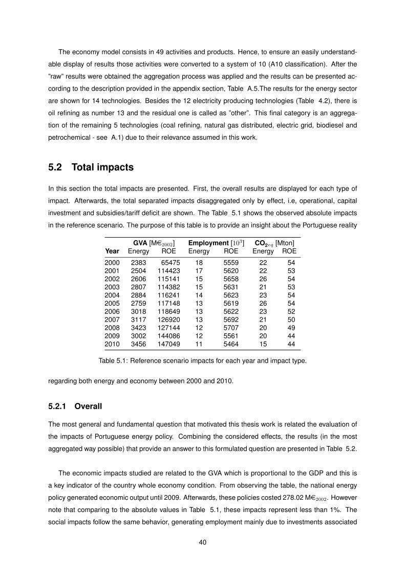
5.2 Total impacts . . . . . . . . . . . . . . . . . . . . . . . . . . . . . . . . . . . . . . . . . . . 40
5.2.1 Overall . . . . . . . . . . . . . . . . . . . . . . . . . . . . . . . . . . . . . . . . . . 40
5.2.2 Economic impacts . . . . . . . . . . . . . . . . . . . . . . . . . . . . . . . . . . . . 41
5.2.3 Social impacts . . . . . . . . . . . . . . . . . . . . . . . . . . . . . . . . . . . . . . 42
5.2.4 Environment impacts . . . . . . . . . . . . . . . . . . . . . . . . . . . . . . . . . . . 42
5.3 Effect disaggregation . . . . . . . . . . . . . . . . . . . . . . . . . . . . . . . . . . . . . . . 43
5.3.1 Operational . . . . . . . . . . . . . . . . . . . . . . . . . . . . . . . . . . . . . . . . 43
5.3.2 Capital investment . . . . . . . . . . . . . . . . . . . . . . . . . . . . . . . . . . . . 48
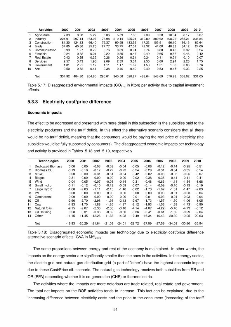
5.3.3 Electricity cost/price difference . . . . . . . . . . . . . . . . . . . . . . . . . . . . . 51
6 Conclusions 55
6.1 Achievements . . . . . . . . . . . . . . . . . . . . . . . . . . . . . . . . . . . . . . . . . . . 55
6.2 Future Work . . . . . . . . . . . . . . . . . . . . . . . . . . . . . . . . . . . . . . . . . . . . 56
Bibliography 57
A List of classifications used 61
xii
Page 13
List of Tables
3.1 Description of symbols used in economy and energy model . . . . . . . . . . . . . . . . . 16
3.2 Structure of the economic model. A= technical coefficients matrix; y=final demand; D and
r’ are primary inputs vectors; x= total output. . . . . . . . . . . . . . . . . . . . . . . . . . 17
3.3 Structure of the energy model. A= technical coefficients matrix; y=final demand; D and r’
are primary inputs vectors; x= total output. . . . . . . . . . . . . . . . . . . . . . . . . . . . 17
3.4 Energy and economy interaction hybrid model. . . . . . . . . . . . . . . . . . . . . . . . . 18
3.5 Hybrid model extension with subsidies and endogenous households . . . . . . . . . . . . 19
3.6 Full integrated hybrid model. . . . . . . . . . . . . . . . . . . . . . . . . . . . . . . . . . . 20
4.1 The model overview characteristics. . . . . . . . . . . . . . . . . . . . . . . . . . . . . . . 23
4.2 Electricity generation technologies. Combined Heat and Power (CHP) allows heat supply
as well. . . . . . . . . . . . . . . . . . . . . . . . . . . . . . . . . . . . . . . . . . . . . . . 26
4.3 Costs structure considered for each technology. The marked numbers (*) consider both
variable and fixed O&M due to their different sources. . . . . . . . . . . . . . . . . . . . . 29
4.4 Thermoelectric power plants in Portugal and their capacities. The symbol (*) is intended
to note that in each year a facility group of 236 MW was closed. . . . . . . . . . . . . . . . 30
4.5 GHG emission factors used per fuel-type/technology in tonnes per TJ of input (Gomez
et al. 2006). . . . . . . . . . . . . . . . . . . . . . . . . . . . . . . . . . . . . . . . . . . . . 30
4.6 Carbon emission prices in current e/ton. From Reinaud (2007). . . . . . . . . . . . . . . . 31
4.7 Job creation data for each technology. From Rutovitz & Harris (2012). . . . . . . . . . . . 31
4.8 SR subsidies. ”Feed-in” tarrifs values in current prices [e/MWh] from 2000 to 2010
(Amorim et al. 2013). . . . . . . . . . . . . . . . . . . . . . . . . . . . . . . . . . . . . . . . 32
4.9 Ordinary Regime. Power Purchase Agreements (PPA) / CMEC values in current prices
from 2000 to 2010 (Amorim et al. 2013). . . . . . . . . . . . . . . . . . . . . . . . . . . . . 32
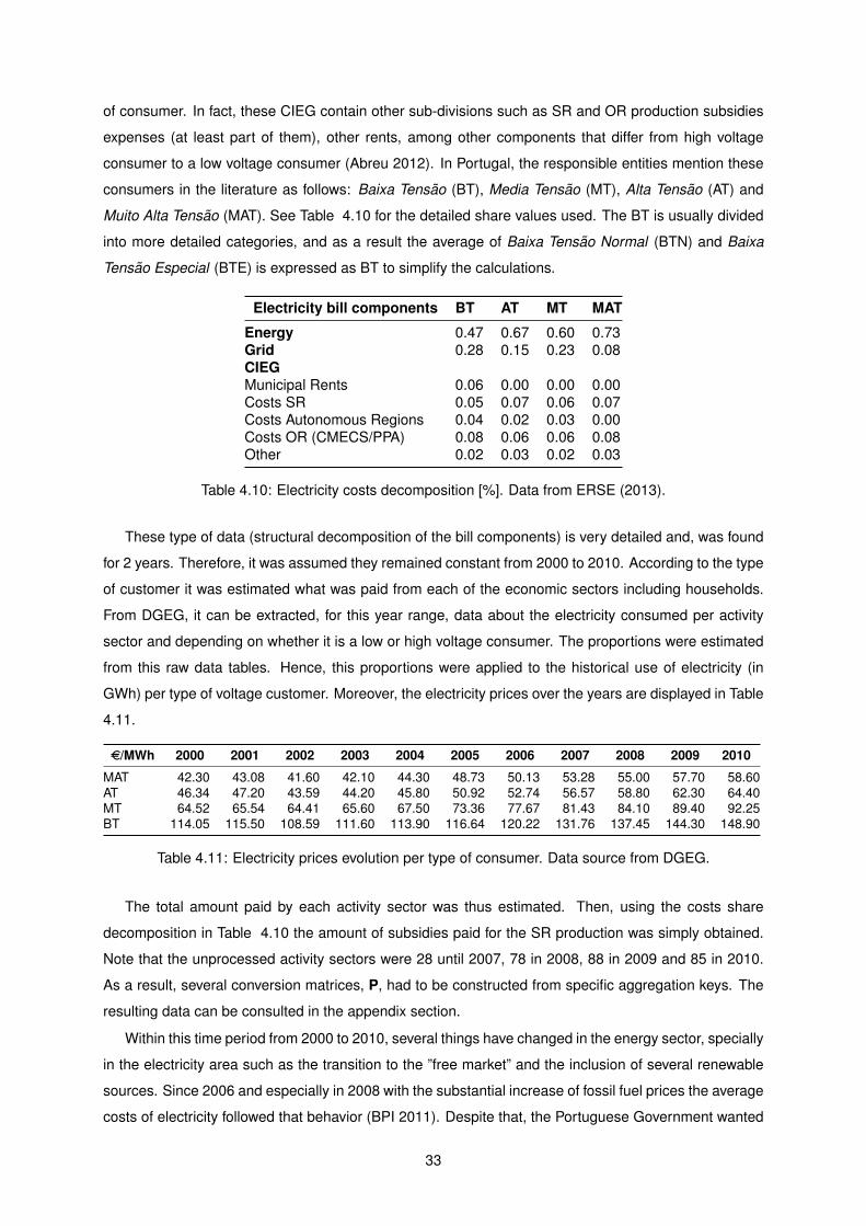
4.10 Electricity costs decomposition [%]. Data from ERSE (2013). . . . . . . . . . . . . . . . . 33
4.11 Electricity prices evolution per type of consumer. Data source from DGEG. . . . . . . . . 33
4.12 Use of economic products by the energy technologies. From Oliveira et al. (2013). . . . . 34
4.13 Most significant fractions of the investment costs breakdown structure per energy tech-
nology. . . . . . . . . . . . . . . . . . . . . . . . . . . . . . . . . . . . . . . . . . . . . . . . 37
5.1 Reference scenario impacts for each year and impact type. . . . . . . . . . . . . . . . . . 40
xiii
Page 14
5.2 Total impacts of the Portuguese energy policy. . . . . . . . . . . . . . . . . . . . . . . . . 41
5.3 Total economic impacts, GVA, by type of effect. Monetary units in Me2002. . . . . . . . . . 41
5.4 Total employment impacts (103 jobs) by type of effect . . . . . . . . . . . . . . . . . . . . . 42
5.5 Total environmental impacts. Emissions of CO2eq in Mton by type of effect. . . . . . . . . 43
5.6 Disaggregated net impacts for the technologies regarding the GVA in Me2002. . . . . . . . 43
5.7 Disaggregated net impacts for activities regarding the GVA in Me2002. . . . . . . . . . . . 44
5.8 Disaggregated employment net impacts (number of jobs) for the technologies. . . . . . . 45
5.9 Comparison between reference and alternative scenarios for employment in activities due
to operational effects. See A.5 for activities description. . . . . . . . . . . . . . . . . . . . 46
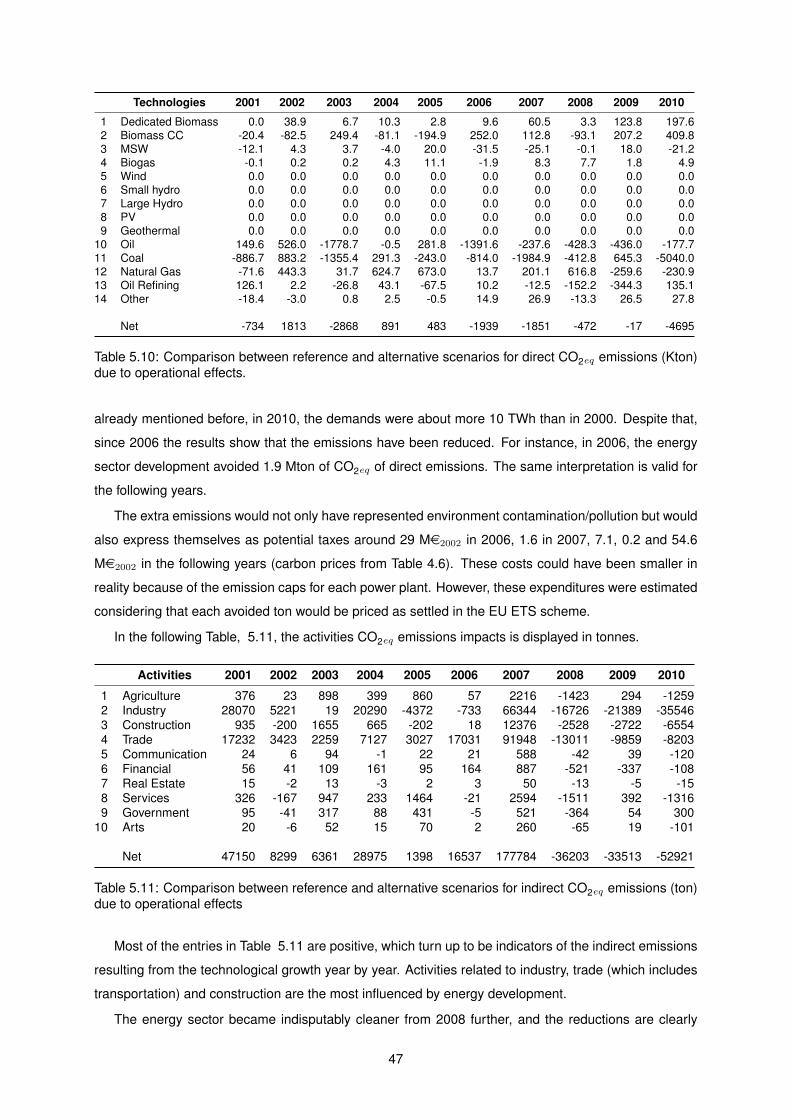
5.10 Comparison between reference and alternative scenarios for direct CO2eq emissions (Kton)
due to operational effects. . . . . . . . . . . . . . . . . . . . . . . . . . . . . . . . . . . . . 47
5.11 Comparison between reference and alternative scenarios for indirect CO2eq emissions
(ton) due to operational effects . . . . . . . . . . . . . . . . . . . . . . . . . . . . . . . . . 47
5.12 Disaggregated economic impacts per technology due to capital investment effects. GVA
in Me2002. . . . . . . . . . . . . . . . . . . . . . . . . . . . . . . . . . . . . . . . . . . . . . 48
5.13 Disaggregated economic impacts per activity due to capital investment effects. GVA in
Me2002. . . . . . . . . . . . . . . . . . . . . . . . . . . . . . . . . . . . . . . . . . . . . . . 49
5.14 Disaggregated social impacts (number of jobs) per technology due to capital investment
effects. . . . . . . . . . . . . . . . . . . . . . . . . . . . . . . . . . . . . . . . . . . . . . . . 49
5.15 Disaggregated social impacts (103 jobs) per activity due to capital investment effects. . . . 50
5.16 Disaggregated environmental impacts (CO2eq in Kton) per technology due to capital in-
vestment effects. . . . . . . . . . . . . . . . . . . . . . . . . . . . . . . . . . . . . . . . . . 50
5.17 Disaggregated environmental impacts (CO2eq in Kton) per activity due to capital invest-
ment effects. . . . . . . . . . . . . . . . . . . . . . . . . . . . . . . . . . . . . . . . . . . . 51
5.18 Disaggregated economic impacts per technology due to electricity cost/price difference
alternative scenario effects. GVA in Me2002. . . . . . . . . . . . . . . . . . . . . . . . . . . 51
5.19 Disaggregated economic impacts per activity due to electricity cost/price difference alter-
native scenario effects. GVA in Me2002. . . . . . . . . . . . . . . . . . . . . . . . . . . . . 52
5.20 Disaggregated social impacts (number of jobs) per activity due to Cost/Price dif. alterna-
tive scenario effects. . . . . . . . . . . . . . . . . . . . . . . . . . . . . . . . . . . . . . . . 52
5.21 Disaggregated social impacts (103 jobs) per activity due to electricity cost/price difference
alternative scenario effects. . . . . . . . . . . . . . . . . . . . . . . . . . . . . . . . . . . . 53
5.22 Disaggregated environmental impacts (CO2eq in Kton) per activity due to electricity cost/price
difference alternative scenario effects. . . . . . . . . . . . . . . . . . . . . . . . . . . . . . 53
5.23 Disaggregated environmental impacts (CO2eq in Kton) per technology due to electricity
cost/price difference alternative scenario effects. . . . . . . . . . . . . . . . . . . . . . . . 54
A.1 List of the 18 energy technologies considered. . . . . . . . . . . . . . . . . . . . . . . . . 61
A.2 List of the 42 energy carriers considered. . . . . . . . . . . . . . . . . . . . . . . . . . . . 61
xiv
Page 15
A.3 List of the 49 economy products considered. . . . . . . . . . . . . . . . . . . . . . . . . . 62
A.4 List of the 49 economy activities considered. . . . . . . . . . . . . . . . . . . . . . . . . . 63
A.5 A10 classification of activities description. . . . . . . . . . . . . . . . . . . . . . . . . . . . 64
xv
Page 17
List of Figures
3.1 Input Output table structure represensation. Based on figure from Gretton (2013). . . . . 12
4.1 Evolution of the accumulated power capacities for each renewable energy technology
considered. . . . . . . . . . . . . . . . . . . . . . . . . . . . . . . . . . . . . . . . . . . . . 27
4.2 Evolution of the accumulated power capacities for each conventional fossil fuel technolo-
gies considered. . . . . . . . . . . . . . . . . . . . . . . . . . . . . . . . . . . . . . . . . . 27
4.3 Evolution of the electricity production share percentage by renewable sources vs. non
renewable (fossil fuel). . . . . . . . . . . . . . . . . . . . . . . . . . . . . . . . . . . . . . . 28
4.4 Special Regime. ”Feed-in” tarrifs values in current prices [e/MWh] from 2000 to 2010.
Data from Amorim et al. (2013). . . . . . . . . . . . . . . . . . . . . . . . . . . . . . . . . . 32
4.5 Use of economy products by technologies (except energy related) in Me2002 by year. . . . 36
4.6 Total investment expenditure in the energy sector related to the maintenance and the
installed capacity in Me2002 by year. . . . . . . . . . . . . . . . . . . . . . . . . . . . . . . 38
xvii
Page 19
List of Abbreviations
AT Alta Tensao.
BT Baixa Tensao.
BTE Baixa Tensao Especial .
BTN Baixa Tensao Normal .
CCGT Combined Cycle Gas-Turbine.
CCOT Combined Cycle Oil-Turbine.
CGE Computable General Equilibrium.
CHP Combined Heat and Power.
CMEC Custos de Manutencao de Equilıbrio Contrat-
ual .
DGEG Direccao Geral de Energia e Geologia.
E3 Environment, Energy and Economy.
EC European Commission.
ENE 2020 National Energy Strategy 2020.
EREC European Renewable Energy Council.
EU ETS European Union Emission Trading Scheme.
FIT Feed-in Tariff.
FTE Full Time Employment.
GCF Gross Capital Formation.
GDP Gross Domestic Product.
GHG Green House Gases.
GVA Gross Value Added.
GWP Global Warming Potential.
INE National Statistics Institute.
IO Input-Output.
MAT Muito Alta Tensao.
MT Media Tensao.
NACE Statistical Classification of Economic Activities
in the European Community.
NPISH Non-Profit Institutions Serving Households.
xix
Page 20
NRES-E Non-Renewable Energy Source Electricity.
O&M Operation and Maintenance.
OR Ordinary Regime.
PCC Pulverized Coal Combustion.
PPA Power Purchase Agreements.
PV Solar Photovoltaics.
RES Renewable Energy Source.
RES-E Renewable Energy Source Electricity.
RNBC Roteiro Nacional do Baixo Carbono.
ROE Rest of the Economy.
ROW Rest of the World.
SCA System of Environmental Accounts.
SR Special Regime.
SUT Supply-Use Table.
xx
Page 21
Chapter 1
Introduction
1.1 Context
Energy produced from renewable sources is becoming a significant fraction of the energy mix in many
countries, as the result of policies that aim to reduce the emission of GHG and mitigate climate change.
International policies applied, as Kyoto protocol, and also at the European Union (EU) level, renewable
energy and carbon mitigation policies have been guided by the European Renewable Energy Council
(EREC) and the European Commission (EC), among other directives and road maps. At the national
level, Portuguese policies on these matters have been guided by Roteiro Nacional do Baixo Carbono
(RNBC), for example. In the Portuguese case, the electricity generation promotion from the renewable
sources, Renewable Energy Source Electricity (RES-E), has been a priority not only due to the environ-
mental concerns but also to increase energy security and diversify our energy supply. Of course, social
and economical considerations play a fundamental role in energy policy (Philbert 2011).
In the last decade Portugal witnessed a substantial increase in the penetration rate of renewable
energies, fueled by high Feed-in Tariff (FIT). As a result, over a short period of time Portugal became a
leader in renewable energy use (IEA 2009). Feed-in tariffs are a part of an energy policy which includes
other financial incentives (National Renewable Energy Action Plan from 2009) and ambitious targets
for the development of hydro power, wind and solar and other technologies. According to the National
Energy Strategy 2020 (ENE 2020), in 2020 Portugal should reduce the energy dependency on imports
to 74%, the RES-E production share should increase to 60%, and the final energy consumption should
decrease by 20%, among others goals such as the creation of 100,000 new green jobs.
The main policy instrument applied in Portugal for the promotion of electricity produced from re-
newable energy sources are the so called FIT. In a FIT scheme, a fixed amount of money per unit of
renewable electricity is paid to the renewable energy producer, irrespective of the market value. This
tariff is an incentive to compensate the higher costs of the RES-E technologies compared to conven-
tional energy production. The value of the FIT is calculated by taking into account the technology,
environmental aspects and the inflation rate. This tariff is fixed for a long time (usually 15-20 years) to
create long term stability for the electricity producers. When considering the electricity sector, one must
1
Page 22
consider both production regimes, the so-called special and ordinary regime. In the Special Regime
(SR), it is included not only the renewable sources (except large hydro power plants) but also micro
production, waste and co-generation, Combined Heat and Power (CHP) both from renewable and other
non-renewable sources. In fact, since 1988 that special incentives and guaranteed purchase prices have
been granted to generators in SR (?) to support the expenses of these emerging technologies. If the
electricity is produced from conventional non-renewable thermal sources (mainly as fuel, coal, natural
gas) and large hydroelectric plants, Ordinary Regime (OR), there are also subsidies to compensate
the high investment costs and support a portion of the financial expenses. They are commonly re-
ferred in the literature as Power Purchase Agreements (PPA) and later in 2004 exchanged by a financial
equivalent fee called Custos de Manutencao de Equilıbrio Contratual (CMEC), designed to guarantee a
pre-establish return on investment over the economic lifetime of the plant. The Portuguese Renewable
Energy Source (RES) policy uses other mechanisms, such as fiscal deductions for heating and cooling
where 30% of the RES equipment costs were deductible; a mandatory biofuels quota in fossil fuels; total
or partial tax exemption regarding the transport sector as the tax on petroleum and energy products (see
EREC Portugal policy review 2009).
The energy sector has developed, and it will continue to grow towards a future where efficiency,
environmental and economical targets meet each other. In fact, according to the National Action Plan
for Energy Efficiency from 2008, Portugal intends to implement energy efficiency measures equivalent to
9.8% of total final energy consumption by 2015. Therefore, the rest of the economy sectors also change
and develop over the years. Hence, the interaction between energy and economy is fundamental to
understand and evaluate impacts such as the ones related to employment and gas emissions. It is within
this present context, that Input-Output (IO) analysis arises and thus the usefulness of this technique to
evaluate economy-wide impacts.
1.2 Motivation
A major limitation in current IO studies of renewable energy is the lack of detailed source data, in par-
ticular for countries like Portugal where some European and even worldwide studies seem to provide
few information. Hence, a major expected contribution of the present study is an improved characteriza-
tion of the production recipe of the energy sector. Furthermore, the energy sector characterization will
contain a larger portion dedicated to existing and emerging technologies for electricity production within
this 10 year time period. This will be accomplished searching for several data sources such as Direccao
Geral de Energia e Geologia (DGEG) and National Statistics Institute (INE) databases and documents
such as the Energy Sources Production Costs and Performance of Technologies for Power Generation,
Heating and Transport (European Commission 2008) although this will be presented in more detail fur-
ther on chapter 4. This work will be mostly turned to a more technological component of the analysis
proposed. In other words, this technological component could be understood as investment, operation
and maintenance costs for each renewable energy source as well as efficiencies, power generation and
capacities, among other factors as capital and labor associated to this sector. Overall, with this improved
2
Page 23
characterization it is intended to establish in a more detailed way the social, environmental and economic
RES impacts on the economy as a whole through our implemented IO model. Therefore, the possibility
to provide an answer to several questions such as the ones announced before, and also analyze them
in an historical context is definitely a motivation boost. Ultimately, disaggregating the energy sector from
the rest of the economy and characterize it with more technologies will allow a enhanced study on the
interaction between energy and economy.
Several issues like the ”green” employment creation, as discussed earlier, are still controversial.
Another issue that is not widely accepted and has been a reason to criticize the government policies
regarding the renewables is the case that the monetary value of these subsidies is not properly deter-
mined (Amorim et al. 2010), and its benefits are not clear to the several axis of interaction, Environment,
Energy and Economy (E3) an social. In order to be able to provide an answer and justify my position
on these issues this study will take place and hopefully will end up being a positive contribute to the
Portuguese economy energy sector characterization.
1.3 Problem Formulation
Although a number of challenges still remain, the renewable energy technologies development has been
undisputed. This is also because in a country with natural conditions such as Portugal, rainfall (for hydro
power) and wind play a main role. As a result, if measured by penetration rate of several renewables
sources, the contemporary Portuguese energy policy has been a great success. But at what cost?
The cost of our renewable energy policy contains both direct and indirect impacts. Direct impacts
are the tax burden required to subsidize the feed-in tariffs and other policy mechanisms, as well as the
increased energy prices supported by consumers and the variation of the energy mix, with a reduced
consumption of fossil fuels. However, there are also indirect impacts, because the purchase structure of
the renewable and conventional energy sectors are different, which means that the impacts in the rest
of the economy will be different. Hence, besides environmental impacts such as the reduction in carbon
emissions, the Portuguese RES policy has also had social impacts such as the creation or destruction
of employment and the increase or decrease in Gross Domestic Product (GDP). Although it is often
claimed that the promotion of renewable energy increases energy security, mitigates climate change
and promotes job creation, the latter result is still disputed (Lamberti & Silva 2012).
The goal of this thesis is to build a hybrid Input-Output model (which will be discussed further) of
the Portuguese economy which integrates a disaggregated energy sector in an existing model of the full
economy and use it to assess a number of impacts. After the necessary data is gathered and the hybrid
model is built it will be used to calculate impacts of the Portuguese energy sector in terms of employment,
added value and greenhouse gas emissions. The costs and benefits of the PortugueseRES policy will
be assessed by comparing the historical impacts of the period 2000-2010 with counter-factual scenarios
in which the observed energy policy had not taken place.
3
Page 24
1.4 Thesis outline
The remainder of this thesis is organized as follows. In chapter 2 it is explained the theoretical founda-
tions about input-output. In the same chapter it is presented the literature review on Portuguese studies
as well as Rest of the World (ROW) case studies. Later, in chapter 3 the Leontief and the the hybrid
units IO model built will be presented. Chapter 2 will be used to discuss the fundamental information
and assumptions steps on gathering and manipulating the data. Then, chapter 5 will handle the results
and the conclusions are provided in chapter 6.
4
Page 25
Chapter 2
Literature Review
2.1 Theory
In order to assess the impact of the renewable energies in the Portuguese context, this study will use
Input-Output (IO) techniques. It is an analytical framework, often known as interindustry analysis, since
its fundamental purpose is to analyze the interdependence of industries in an economy represented as
a whole.
The first attempt to describe the way economy works in an analytical way was performed by Francois
Quesnay, a French economist known for developing a first approach of this technique which he published
in 1758 as Tableau Economique (economic table). In addition Leon Walras, a French mathematical
economist presented Elements of Pure Economics where he explained the general equilibrium theory in
1874. This theoretical model, in a brief description, seeks to explain the behavior of supply, demand, and
prices in a whole economy linear system with several interacting markets, considering that the long term
prices will tend to be in equilibrium. The problem was that, despite their valuable work, no one could
employ their findings to the solution of problems. Wassily Leontief was influenced by these previous
works that could be seen as a forerunner to Leontief’s own concept. Due to his work (Leontief 1936,
1941) he was later credited with the development of this framework which granted him the Nobel Prize
in Economics in 1973. His major contribution was to simplify Leon Walras’s formulation in order to make
the computation feasible and due to his work on input-output tables and its development as a model the
Input Output technique is often known as Leontief’s own model.
The Leontief demand-driven quantity input-output model allows the quantification of the final demand
stimulus in primary production factors (Miller & Blair 2009). This model allows to identify the impacts that
arise from changes in the intermediary flows between industries (and products) as a result to a variation
in the final demand. It is a widely used model for its numerous applications and input-output may be used
recurring to units other than monetary. In fact, Leontief continued to explore his framework regarding
physical units (Leontief 1989), and many researchers such as Duchin (1992) and Cleveland (1999) have
extended the original framework in the direction of areas such as industrial ecology and economics
ecologic. In addition, environmental concerns can also be addressed as, for example, pollution that
5
Page 26
should be related in a measurable way to a particular consumption or production process (Leontief
1970). With the contribution of several researchers and the continuous work being developed, the
utility about input-output to numerous disciplines is unanimously recognized. Hence, energy input-output
analysis is no exception.
Energy was and still is a crucial factor on production for many industries over the world. The focus on
the role of energy in the economy became a priority, specially during fossil fuel crisis and climate change
in recent years (Miller & Blair 2009, pag. 400-401). The early developments were achieved by several
authors and their work such as Strout (1967), Cumberland (1966), Bullard & Herendeen (1975), among
others. Also, the concern and technology changes worldwide has boosted several works. Although it
seems to be only a recent issue, it is not. Such studies have been guided also in the past years by
authors such as Just (1974), Gowdy & Miller (1968) and Herendeen & Plant (1981). In this work, it
is proposed to built and hybrid units model (both monetary and energy units). The so-called ’hybrid
units” approach was first introduced by Bullard & Herendeen (1975) to address the limitations about the
simplest approaches.
The development and growth of new energy technologies has encouraged several studies. As a re-
sult, numerous studies have been conducted either for Portugal or other countries and regions regarding
the use of IO for the evaluation of the impact of renewable resources use in the economy. In the next
sub chapters some of them will be briefly presented and discussed first for many countries or regions
around the world and then the focus will be on Portugal case studies in the literature.
2.2 Rest of the world case studies
Input-output analysis and similar techniques have been providing some interesting results on the im-
pacts caused by the renewable energy sources sectors. Social impacts are related to employment or
sometimes referred as clean jobs creation. One of these studies was published in 2013 by the Na-
tional Council of Applied Economic Research (NCAER 2013). In this, they estimated the number of
jobs created in the wind sector for Gujarat State, India. This study was motivated due to the increasing
importance of the wind technology energy production (80% of RES-E share just by wind in 2010). In
addition, the importance on understanding the growth on the RES sector and its impacts on all other
sectors of the economy fueled this study. It was necessary to construct their Gajurat state IO table and
with that purpose they created a 7 sector (Agriculture, Mining, Manufacturing, Construction, Electric-
ity, Other Services and Public Sector) transaction matrix based on the All-India-Input-Output table from
2006-2007 (most recent data available) and disaggregated the wind energy sector from the electricity
sector, making it an 8 sector table. To obtain the data required for wind sector, surveys were taken
in consideration and questionnaires were done to workers and wind entities (which were concluded in
2012). The state table was adapted for 2009-2010 due to the available data. Wind energy plants re-
quire heavy expenditure in construction, manufacturing, infrastructure, etc. Therefore, this fact is easily
observed in the employment results, as an unit increase of the wind energy output generates a total em-
ployment of 0.334 man-year as compared to 0.268 man-year for conventional electricity. Even though
6
Page 27
the assumptions made to gather the data necessary to build the state table and the usage of older in-
formation could cause a significant deviation in the results, the study proved to be an interesting way to
provide an insight about the wind sector impacts on the state level regarding the job creation.
Another highly controversial issue is the government subsidies and other incentives that are applied
to the renewables sources with the energy sector. This following case study considers Spain which had
clearly defined goals to enhance the RES sector by 2010, such as to reach 12% penetration by these
sources in the energy market and 20% of electric production. Alvarez (2013) provided an answer to
the question of what is the price to pay while making efforts to promote large numbers of green jobs.
In fact, the European current policy and strategy for supporting the so-called ”green jobs” or renewable
energy dates back to 1997, and has become one of the principal justifications for U.S. ”green jobs”
proposals. The study calculates that since 2000 Spain spent 571,138 e to create each green job,
including subsidies of more than 1 million e per wind industry job. Moreover, creating those jobs also
resulted in the destruction of nearly 110,500 jobs elsewhere in the economy, or 2.2 jobs destroyed
for every job created by the renewables. In other type of analysis, they estimated that each ”green”
megawatt installed destroys essentially 8.99 jobs by photovoltaics, 4.27 by wind energy and 5.05 by
mini-hydro in the rest of the economy. It is interesting to note that the prices for renewables to generate
electricity is far above market prices, resulting in a vast amount of capital that could have been otherwise
allocated in other sectors in the economy. However, these costs do not appear to be unique to Spain’s
approach but seem instead inherent in schemes used to promote renewable energy sources in other
countries.
The whole idea of ”green jobs” and they meaning is vastly discussed in the paper published by Winter
and Moore (Winter & Moore 2013). It is proposed a better way to measure very clearly and reliably
whether we are harming the environment or not. It is based on measuring the energy use intensity and
emissions intensity, even though it is not as political appealing as promising ”green employment”, which
is considered an illusion and an arbitrary concept. This study was conducted taking in consideration the
Canadian context on 20 sectors describing the economy and it was found that the majority of Canadian
industries improved their emissions intensity between 1990 and 2008.
Investments on the energy sector is also an important effect to consider. Markaki et al. (2013)
provides in his work a specific study about the impact of clean energy investments on the Greek economy
between 2010 and 2020. These impacts are evaluated using the IO analysis on 20 industrial sectors of
the economy. the required data was gathered from the Eurostat’s domestic input-output table from 2010.
Furthermore, in their IO model both direct, indirect and induced effects are considered. Of course that
Greece, as a part of EU, also has its ambitious goals regarding environmental and energy objectives to
be achieved by 2020. Therefore, it was proposed first to calculate the amount of capital investments in
the renewable energies, by industrial sector, that the country would need in order to satisfy a number
of energy and environmental targets adopted in the context of the European Commission’s energy and
climate change package. Afterwards, the macro-economic impacts of these ”green” investments in the
whole Greek economy would be calculated. In their results, the required investments would reach the
amount of 47,9 billione over the 10 year range period. Simultaneously these investments would not only
7
Page 28
increase the nation production by 9,4 billion e as it would also create 108,000 Full Time Employment
(FTE) for the same period. And from these results obtained for Greece, one can identify that large scale
exploitation of clean energy technologies to achieve the European Commission goals would create a
large volume of output and employment.
When completing a study about energy and employment several factors should be considered, such
as labor intensity of renewables, cost increases and availability of investments, counting job losses, job
quality and skills, model assumptions and sources of information Lamberti & Silva (2012). In this, R. J.
Lambert and P. P. Silva discuss these factors that affect job estimates as well as how should job creation
be measured. It is important to take in consideration that not only each technology has its own job ratio
(e.g. per MW installed) but also that ratio changes from country to country, meaning that one should
be cautious when using those data informations. As an example, consider Denmark because it has a
large wind turbine manufacturing sector (high job rate). however most of the components are exported
and this falsely inflates the job per MW installed ratio. Furthermore, when obtaining results, renewable
energy should not be encouraged solely because of a perceived benefit to employment, nor should it be
rejected without considering other potential benefits (E3 interactions plus social).
In the literature there is also some studies to measure the impact of policies strategies in the labor
market due to the high level of unemployment. One example is the work conducted by Lehr et al.
(2007). In this paper it is developed an IO vector for the renewable energy sector based on the results of
an questionnaire (more than 1000 interviews). The process is based on the calculation of gross and net
effects of two difference policy scenarios for Germany until 2030. The IO tables of the German Federal
Statistical Office consist of 59 production sectors and the difference from earlier studies resides in the
modeling, which accounts explicitly of exports and foreign trade effects.
One thing that is also fundamental when applying these IO models are the units used and their
influence on the desired analysis. An analysis in monetary units can be done, or instead in physical
units, but also a mix of both, i.e. hybrid units. Therefore, energy sectors or commodities of hybrid IO
tables for energy are in physical units which are usually reported in joule, while non-energy sectors
or commodities are in monetary units. These differences and limitations are discussed by Liang et al.
(2010) and it is proposed an hybrid physical input-output model for energy analysis to study energy
metabolism taking Suzhou in China as a case of application. This improved model calculates energy
resources in both energetic and mass units and air pollutants in mass units simultaneously from the
perspective of energy and mass balance, which is said to be beyond the reach of current IO tables for
energy. The model can be used both as an accounting tool (it provides a measure on the environmental
impacts) or as a forecasting tool (e.g. for Suzhou in 2020). Regarding the data used, for example the
energy consumption and domestic extraction data of each 25 sectors used came from the 2006 Suzhou
Statistical Yearbook (SBS). Among other results, it is referred that the energy consumption of Suzhou
(where manufacturing dominates the energy consumption) relies mostly on energy imports and it will
keep relying in the future years.
Sometimes a sensitivity analysis should be taken in consideration in order to identify the potential of
one or various coefficients to change the desired output significantly. These sensitivity analysis can be
8
Page 29
combined with IO methodology to study several impacts, as for example environmental related ones, as
CO2 emissions (Tarancon & Rıo 2007). In their work, it was suggested that emissions are connected
to the IO productive relationship within an economy; to the CO2 emissions intensity of sectors and to
the structure of final demand on the different sectors. This methodology was applied to the Spanish
case and for that, data based on the Spanish IO table was used. This table was built from the National
Statistical Office for 1995 and the 1995 CO2 emissions vector (disaggregated by activity branch), also
published by INE as part of the System of Environmental Accounts (SCA). The study ended up with
44 production sectors and the sensitivity analysis revealed that emissions in the energy, residential and
transport sectors should be tackled if total emissions are to be significantly reduced.
In conclusion, there are a relative large amount of studies which are based on the IO method to
study energy. Some of them with a more financial and economical analysis, others oriented towards
social and environmental analysis and so on. The wide range of uses of this IO technique and models
implemented from this one is well reproduced in the literature as we have seen in the selected studies
discussed above. The results are not entirely global and some case studies seem to present different
conclusions, depending for example on the country/region, policies applied and model implementation.
2.3 Portugal case studies
In the beginning of the review it was said that these impacts by the renewable energy sources were also
studied in the Portugal case, although there are not that many studies under this conditions. Neverthe-
less, social effects, such as employment, seem to be an recurring subject worth studying. Consequently,
Silva et al. (2012) claimed that employment effects and green energy policies call for more concrete ap-
plied research. Therefore, the aim of this work was to contribute the renewables discussion using the IO
modeling approach. Considering that, Portuguese data used was based on the symmetric tables pro-
duced by the Department of Foresight and Planing for the year 2008 (Dias & Domingos 2012). For this
study this data was adapted to 64 production sectors. For Portugal and most countries the employment
data on FTE is not directly available, and so for this study several sources were taken in considera-
tion to gather the job ratios per RES technology. Continuing the implementation, new IO vectors have
been constructed for each RES source with their respective intermediary input structure allocation and
then the direct and indirect employment were estimated. Afterwards, two case scenarios were consid-
ered: the RES basic equipment is domestically produced and that same equipment is imported. These
different scenarios allowed to conclude that the production of a significant part of the manufacturing
activities domestically is an ideal prerequisite for maximizing the positive socio-economic effects of the
RES development in the Portuguese economy. In fact, this same conclusion is also achieved by Oliveira
et al. (2013) using a optimization multi-objective model to optimize the economic growth (gross domestic
product); level of employment and RES production creating different scenarios. Considering the 105
thousand ”green” employment expected for Portugal by the NES 2020, this goal would only be achieved
if induced effects were considered in the analysis.
In chapter 1, it was stated the main policy to promote the renewable energy sources are the feed-in
9
Page 30
tariffs. This system has been in place in Portugal since 1988 and since then several changes have
occurred. One example, occurred in 2001 where the tariffs began to be differentiated by type of renew-
able technology. Proenca & Aubyn (2013) intended to provide an empirical assessment of the economic
and environmental effects of the Portuguese FIT policy to promote RES-E generation according to the
national target of 45 % RES-E in 2010. The methodology used in their quantitative analysis is a hybrid
top-down/bottom-up Computable General Equilibrium (CGE) model, once it contains both technological
foundation of bottom-up models and the economic richness of top-down general equilibrium models.
These characteristics would allow to study the E3 interactions in an integrated and consistent way. In
addition, this approach had never been applied to assess the FIT scheme effects in the Portuguese
economy. This model approach is explained in detail by Proenca & Aubyn (2009). The model framework
dimensions consists of: 18 production sectors/commodities (14 non-energy and 4 energy); final demand
drivers; 7 representative electricity generation technologies; primary factors (labor, capital and natural
resources) and national and ROW regions. The results show that these tariffs lead to a diversification
of the energy mix with a large deployment of renewable energy source illustrating also the shift from
high-carbon fossil fuel technologies towards carbon-free sources. Furthermore, not only the FIT policy
modifies the national production structure of the national electricity sector as described before but it also
makes it less dependent on energy imports. Of course, it also makes it more costly for household and
other activities as they support the part of subsidies (and not for the producers of RES-E).
It is also interesting to understand how the population reacts to the emerging of theses renewable
technologies in the economy, because the subsidies to special and ordinary regime are supported by
consumers (households and activities). In other words, the level of acceptance for each technology is a
substantial social factor that proves itself to be relevant in the deployment of renewable energy sources.
In general, Portuguese residents are quite aware of the RES, and even though some do not understand
that these sources increase the electricity bill due to the tariffs, in the ones who do realize it there
is a tendency to still be favorable to the projects implementation which boosts the social acceptance
regarding these technologies. These results, among others, were obtained by Ribeiro et al. (2013) in a
survey conducted in for Portugal on this subject.
In fact, the studies for Portugal are not that many and there is still a substantial margin to improve and
keep the development of further studies. For the study proposed it is intended to build a hybrid Input-
Output model of the Portuguese economy which integrates a disaggregated energy sector in an existing
model of the full economy. Therefore, the results will hopefully be more accurate and conclusive as the
energy sector will be more detailed. In addiction, as mentioned in chapter 1, the model will be used
to calculate employment, gross value added and greenhouse gas emissions impacts of the Portuguese
energy sector and compare them with the counter-factual scenario in which the observed energy policy
had not occurred the way it did.
10
Page 31
Chapter 3
Method
3.1 Fundamental concepts
Within this section, the fundamental basic concepts are presented and discussed. It begins with a
introduction to explain the Leontief model and its inherent formal objects. Then, the advantages and lim-
itations are provided to enhance the knowledge about the use of input output analysis on problems such
as the ones proposed for this work. Consequently, the use of multipliers, they meaning and relevance is
discussed. In the same subsection, the relation between multipliers and the impacts to be assessed is
revealed (recurring to expressions to be used ahead on calculations).
The standard notation used further on this thesis is based on uppercase bold letters to denote matrix
objects, while bold lowercase letters refer to vector objects in column format (transposed objects are
followed by ’).
3.1.1 Leontief model
In order to understand the Input-Output model approach to the problem proposed it is necessary to
explain and go through a couple of fundamental introductory concepts. Note that this model consists
of a system of linear equations, each one of which describes the distribution of an industry’s product
throughout the economy. In fact, Leontief was the first to use matrix representation. An interindustry
transaction table is considered in which all the IO model information is contained. Basically it concerns
the flow of products or goods from the producers to other sectors, considered consumers. It allows to
see how dependent each sector is on every other sector. Therefore in this table, the rows describe the
distribution of a producer’s output throughout the economy and the columns describe the composition of
inputs required by a particular industry to produce its own output (Miller & Blair 2009). In a simple way,
the IO table can be represented in quadrants as seen in Figure 3.1.
Adding the several values in the rows across quadrant 1 and 2 (adding its sales of goods or services
for intermediate use by other industry and for final use) it is possible to obtain the total output for an
industry. This same output can also be found by adding its own use of goods and services (its inter-
mediate inputs) and primary inputs of labor and capital to production (that is, down quadrants 1 and 3).
11
Page 32
Quadrant 1Intermediate inputs
to production
Quadrant 2Final demand
Quadrant 3Primary inputs to
production
Quadrant 4Primary inputs to
final demand
Total output
Total output
Figure 3.1: Input Output table structure represensation. Based on figure from Gretton (2013).
For this reason, the row and column sum of these tables have to match as a validation process step.
The center-piece of the system is the the industry by industry intermediate inputs matrix Z (in quadrant
1). Additionally it is important to mention clearly what final demand means because it will be a very
important definition to take in account when applying this type of analysis (as seen in chapter 2, final
demand is the exogenous stimulus to our system). Therefore, consider that final demand is referred as
the demand of external units, which tends to be much more to goods to be used than to be applied as
input to an industrial production process.
There is another term that is relevant to mention, as it was already described above without acknowl-
edging it, and that is usually known as the interindustry inputs or intermediate inputs, zij (which fills the
intermediate inputs matrix, quadrant 1). These are the designation for the monetary values of the trans-
action between sectors i to each other sector j. Hence, the total output production xi can be obtained
the following way:
xi =
n∑j=1
zij + yi (3.1)
Introducing the technical coefficient matrix:
A = Zx−1 (3.2)
Each element of A, aij = zij/xj , is the technical coefficient ratio. This is viewed as a relationship
between a sector’s output and it’s input, meaning how much of good or services from sector i are
required to produce one unit of output in sector j. When using this expression, equation 3.1 simply
becomes:
xi =
n∑j=1
aijxj + yi (3.3)
These are mathematical relations that arise from a logical point of view, but the model itself appears
assuming that these technical coefficients are fixed in time. In other words, input proportions between
12
Page 33
different economic sectors are fixed and do not change significantly in the short-term.
x = (I− A)−1y = Ly (3.4)
In this, L = (I − A)−1 is known as the Leontief inverse or total requirements matrix, in which each
matrix component lij represents the total amount directly and indirectly needed of good or service i to
deliver one unit of final demand of good or service j. These assumption allows us to establish a way
to compute the output of each sector, as for example, the economy response to changes in the final
demand stimulus y. Therefore, this model provides the possibility to assess impacts on primary factors
such as employment, GHG emissions, value added, among others.
Advantages and Limitations
Now that we have seen a brief description of the IO model, it is necessary to present the reasons why
this type of analysis should be appropriate to the problem considered on measuring the impact of the
energy sector in Portugal. In order to construct an IO table it is required a lot of data, which is not easy
to gather, and so, these methods are usually used on a national scope rather than on a local or regional
level. Hence, it is possible to identify some advantages regarding these tables:
• The data is usually comprehensive and consistent. These IO tables encompass all the formal
market place activity that occurs in the economy, allowing its representation as a whole regarding
the flows of goods and services industries trade with one another. The several data sources that
are needed to build these tables and to ensure their completeness and internal consistency makes
them probably the single most comprehensive and complete source for economic data for most
countries. As a consequence, IO tables frequently play a fundamental role in the construction of
the national accounts, which are the implementation of several accounting techniques to measure
the economic activity of a nation.
• The nature of IO analysis makes it possible to analyze the economy as an interconnected system
of industries that directly and indirectly affect one another, tracing structural changes back through
industrial interconnections. This is especially important as production processes become more
complex, requiring the interaction of different sectors in these processes. As a result, this model
is appropriate in a way that changes occurring in domestic demand will not only affect the industry
providing that good or product but also the suppliers to that industry, for instance it is possible
to measure the loss in one determined sector due to the growth of another. In other words, IO
techniques trace these linkages from the raw material stage to the sale of the product as a final,
finished good. Therefore this model also has the very important ability to capture not only the
direct effects, but also the indirect and even induced effects.
• The design of input-output tables allows a decomposition of structural change which identifies
the sources of change as well as the direction and magnitude of change. This means that the
model enables changes in output to be linked with underlying changes in factors such as exports,
13
Page 34
imports, domestic final demand as well as technology. This permits a consistent estimation of the
relative importance of these factors in generating output and, for example, employment growth on
the several sectors.
Nowadays, this type of impact analysis has become important to all the highly-industrialized countries
in economic planning and decision making due to several characteristics mentioned before. However,
one must also consider the associated limitations included on the usage of input-output.
• Technical coefficients are assumed to constant over time meaning that the amount of each input
necessary to produce one unit of each output is constant. The amount of input purchased by
a sector is determined solely on the level of output. No consideration is made to price effects,
changing technology or economies of scale. Therefore, the model assumes that the same relative
mix of inputs will be used by an industry to create output regardless of quantity.
• Each industry is assumed to produce only one type of product. For example, the automobile
industry produces only cars. The distribution and sale of this product is fixed.
• Each product within the industry is assumed to be the same. Also, there is no substitution between
inputs. The output of each sector is produced with a unique set of inputs.
• It is assumed that there are no constraints on resources, meaning that supply is considered infinite
and perfectly elastic.
• It is assumed that all local resources are efficiently employed. There is no underemployment of
resources.
• Timeliness of input-output data. Due to the several sources needed to construct these tables, there
is a long time lag between the collection of data and the availability of the tables.
In conclusion, IO models have commonly been applied to evaluate targeted economic policies and
to estimate short and medium term employment impacts. Actually, it is a widely used as a very useful
method capable of simulating almost any conceivable economic impact.
3.1.2 Multipliers and impacts
There are some ratios, also known as multipliers, which are used to estimate the effects of exogenous
changes on: output of sectors in the economy; income earned by households in each sector due to
the new output; social effects (employment) and value added generated across sectors (Miller & Blair
2009, pag. 243-244). These are some of the most frequently used types of multipliers. Another type
is related to environmental concerns, such as GHG emissions which will be evaluated in this work.
Before explaining how do these multipliers will be obtained and their meaning, it is proposed to first take
a look at the concepts behind direct, indirect and induced effects. To begin with, consider there is a
change in the final demand. As a result, there will be changes in the output of the producers to meet
this final demand increase, which are known as direct effects. As these producers increase their output,
14
Page 35
there will also be an increase in demand on their suppliers and so on up the supply chain and these
changes are known as indirect effects. Then, as a result of the direct and indirect effects mentioned
before, the level of household income throughout the economy will increase as a result of increased
employment, for example, and a proportion of this increased income will be re-spent on final goods and
services describing what is known as induced effects. It is important to mention the work of Miyazawa
(1976) on endongenizing the households in an input-output model to reproduce these induced effects
and generate various multipliers matrices.
In the Leontief model, the impact of one euro worth of final demand of product j on the use of a
primary factor (as employment for instance) of sector i is given the multiplier Mij :
M = diag(r)L, (3.5)
where ”diag” is a diagonal matrix and r is the direct primary factor coefficients. The r coefficients vector is
obtained dividing each element of the vector for the corresponding element in the original output vector
x. Then ri represents the amount of primary factor used per unity of output of industry i. Moreover,
the total impact of final demand j on production factor i can be obtained by the product riLijyj . From
3.5, in algebra standard notation, the total impact mentioned before can be simply obtained by the
following product: My. However, for further impacts discussion it is important to keep in mind the simple
expression 3.4 (x=Ly). The reason for this reminder is that this model responds to an exogenous
stimulus, thus x is the variable that will determine the impact b = diag(r)x.
It is intended to present more than one scenario for the historical analysis, hence every year from
2000 to 2010 will have an alternative scenario in addition to the reference one (the so-called ”real case
scenario”). The operational, capital investment and subsidies related to the tariff deficit effects (electric-
ity cost/price difference) on the economic, social and environment impacts are obtained from alterna-
tive scenarios. Furthermore, each effect has different methods of obtaining the appropriate alternative
scenario. The net values comparing reference to alternative scenario are obtained from the following
expression:
∆x = xR − xA (3.6)
The way that xA is obtained depends on the effect desired. These methods are explained further for
each case in the subsection 3.2.3. Obtaining ∆x from expression 3.6, the difference between reference
and alternative scenario impacts are calculated as follows:
∆b = diag(r)∆x (3.7)
In this case, calculating ∆b allows a relative interpretation about impact r on both reference and al-
ternative scenario (as a comparison result). Given the possibility that if the absolute values may not
correspond exactly to the reality, using differences enhances the process of understanding the behavior
of the full model in response to certain desired stimulus and/or effect.
15
Page 36
3.2 Structure of the model
In this subsection it is explained the whole model construction process. First it is presented a description
about the structure of the isolated energy and economy models. Secondly, the first integrated hybrid
model and the following extensions are explained as well as their composing blocks. Therefore, the
modifications required to calculate the desired impacts from the selected effects are still discussed.
3.2.1 Economic model
In spite of presenting and explain only the final hybrid model, it is rather appealing to introduce first the
economic and energy isolated models. Hence, lets consider first the economic system. This model has
49 products and 49 activities sectors. In order to better understand the following steps it is helpful to
note that an IO system is a network of causal links. This means that the whole system is represented by
a set of nodes (e.g., as industries or products) and a set of arcs that connect these nodes to each other
(e.g., intermediary flows referring to activities using products and also producing them). In particular,
this model main quadrant (Z, intermediary matrix) is built with a Supply-Use Table (SUT) framework.
The use matrix has information regarding the uses of products by the industries. On the other hand the
supply matrix refers to products made by the activities. This being said, in table 3.1 the description of
symbols used further can be observed and in table 3.2 it is possible see the schematic representation
of this whole economic model. The APA block is the use matrix and the AAP is the make matrix.
Symbol Description
P Economic productsA Economic activities or industriesM Trade marginsC Energy carriersT Energy technologiesK Capital investmentH HouseholdsS Subsidies
Dom Domestic productionL Net Losses on conversion
Imp ImportsVA Value added
Emp EmploymentGHG Green house gas emissions
Table 3.1: Description of symbols used in economy and energy model
The shaded areas contain the matrices where information is located. The units here in the main
blocks Z, D, Y and X are simply monetary. It is important to know if the monetary flows, i.e, prices, are in
purchase or basic terms. Purchaser prices include the trade margins and the reason they are included
in the Z block full matrix is only a compatibility issue. Therefore, the equality between sum in rows and
columns still has to remain valid. The block r’ has information relatively to employment (obviously with
no units) and GHG emissions in physical units (Mton).
The detail in the total final demand y is accomplished with 5 different categories. As a result the
16
Page 37
A P A M Y XP -AM +
DImpVA
Xr’EmpGHG
Table 3.2: Structure of the economic model. A= technical coefficients matrix; y=final demand; D and r’are primary inputs vectors; x= total output.
initial total exogenous stimulus is composed by households expenditures; Non-Profit Institutions Serving
Households (NPISH); government; Gross Capital Formation (GCF) and exports. In the hope that there is
nothing wrong with this built system, after checking the row and column sums, one can perform another
test. That is, compute the technical coefficient matrix using equation 3.2, A and then the Leontief’s
inverse, L, from equation 3.4. Afterwards, the Leontief model equation is applied and as a result it is
expected that with the final demand data, y, the output vector obtained matches with the one used to
calculate the A matrix. In the final analysis it is possible to be sure that there these two validation criteria
mentioned above are fulfilled (calibration process).
3.2.2 Energy model
The hybrid units model, as it has been mentioned is composed by information in different units. With
this in mind, the energy model hereby presented is in units of energy, tonnes of oil equivalent (toe) for
instance. Table 3.3 shows the overview of the isolated energy model structure. It is possible to identify
some similarity with the previous economic structure. This means that several blocks have the same
meaning such as, final demand y, total output x, and primary factors input vectors r’.
A C T Y XCT
DDomImp
L -
Xr’EmpGHG
Table 3.3: Structure of the energy model. A= technical coefficients matrix; y=final demand; D and r’ areprimary inputs vectors; x= total output.
17
Page 38
The description of these new symbols can be found in Table 3.1. If the previous model was well
understood, and hopefully nicely explained, this energy one would be another simple step towards our
final stage. Consider the full technical coefficient matrix presented above, A. This matrix is built with
two blocks, use and make (supply’s transpose) matrices. The first , ACT has information on how the
energy technologies use the different energy carriers (in energy units), and logically the make matrix
block, ATC , connects technologies to carriers concerning their production and supply (just like activities
make products, technologies make carriers). All the other blocks left uncolored are filled with 0’s. It
is important to have the clear definition of energy carriers and not mistake them with primary energy
sources. From now on, note that when carriers are mention it is referring to the energy form produced
by the energy sector using primary energy sources.
The energy model itself is made with 42 carriers and 18 technologies. In the D matrix, it can be
found the domestic production, imports and the net losses through the transformation process (e.g,
electricity production). The final demand vector is composed by a merge of data accounting the exports,
stock variation, corrections and final consumption by households as well other activities (i.e. 5 different
categories). All things considered, the same two validation tests as before (Leontief’s model test and
matching row and columns sums) were performed resulting in a functioning energy model. Note that the
matching of row and column sums has to be analyzed and checked in this phase because when hybrid
units are involved and the full model is developed this is no longer valid (different units in columns).
3.2.3 Hybrid model
Operational (O&M) effects
It is provided in Table 3.4 the first extension of the hybrid model do assess these operational effects.
Two extra blocks are inserted where interaction between energy and economy is provided. The block
ACA contains the use of energy carriers by all of the 49 economy activities considered. The block APT
reefers to the use of economy products by each of the 18 technologies. The first block mentioned is in
energy units (toe) while the second is in monetary units (Me).
A P A C T Y XPACT
r’
Table 3.4: Energy and economy interaction hybrid model.
In this, to calculate the impacts including only the basic energy and economy blocks with O&M costs,
the technical coefficient matrix A is divided in two blocks: ARROE and AR
E .
To assess the operational effects, O&M, each alternative scenario considers that the energy sector
remains constant from the previous year to the present one, i.e., there is no technology evolution (tech-
18
Page 39
nical coefficient matrix AE does not change). As a result, the output variables for the reference scenario
”R” and alternative ”A” are given by:
xR = LyR (3.8)
xA = L∗yR (3.9)
In which L∗ = (I − A∗)−1 and A∗ = [ARROE |A
AE ]. This technical coefficient matrix is therefore built
with both the reference year t economy block, ARROE , and the t− 1 energy block, AA
E (as an alternative).
Naturally, from this, the ARROE block includes the products and industry/activities columns and AR
E the
carriers and technologies respective columns. It may be useful to analyze the results as differences:
∆x = xR − xA = (L− L∗)yR (3.10)
The resulting ∆x can be used in the expression 3.7 to obtain the economic, social and environmental
impacts due to the energy technology mix development over the years.
Electricity cost and price difference effects
The following extension includes the households endogenous and the energy subsidies spent on elec-
tricity producing technologies. As a result, a couple of selected modifications were processed to obtain
the extended hybrid model shown in Table 3.5.
A P A C T H S y xPACTHS -
r’
Table 3.5: Hybrid model extension with subsidies and endogenous households
The AST block considers the subsidies received by the energy technologies (electricity producers).
The tables composing these blocks for each year are obtained from processed and manipulated data
explained with detail in chapter 4. The AAS and AHS blocks are the amount that is paid for subsidies
either by ROE activities, A, or by households, H. Note that these 2 group of blocks must have different
signs in the technological matrix to represent the different flow direction either by receiving or paying
processes. Hence, to simplify, the AST is negative as the AAS and AHS remain positive elements of the
full A matrix.
The blocks APH and ACH describe the use of products and carriers by the households. To explain,
consider that endogenous households column in the intermediary flow matrix is denoted as ZH :
19
Page 40
ZH =s
Wtoty∗, (3.11)
where s is the amount of subsidies paid by households and Wtot is their total wages received. Also,
y∗ represents the total final demand vector before the endogenizing process. It is important to note that
the total households final consumption is a sum of endogenous and endogenous vectors:
Htot = Hendo + Hexo (3.12)
The endogenous component is already calculated from 3.11 (Hendo = ZH ), thus the real exogenous
final demand vector will be y = y∗ − Hendo. The process of obtaining the impacts in this case is similar,
with the same alternative scenario method.
To assess the effects on subsidies and the tariff deficit the alternative scenario considers endogenous
modifications. The main question here is: what would happen if the subsidies were fully reproduced in
the electricity bill and no tariff deficit would occur? In other words, the cost/price difference of electric-
ity producing is considered zero in alternative scenario. Therefore, these effects are captured on the
resulting impacts.
Therefore, with the presented hybrid model, this question can be answered by stating that alternative
scenario considers the blocks AAS and AHS to be consistent with the block AST (every subsidy received
is really supported by consumers). Naturally APH and ACH are recalculated for the alternative scenario.
To summarize, the ∆x is obtained just as for the operational effects. The difference is in the alterna-
tive scenario considerations.
Capital investments effects
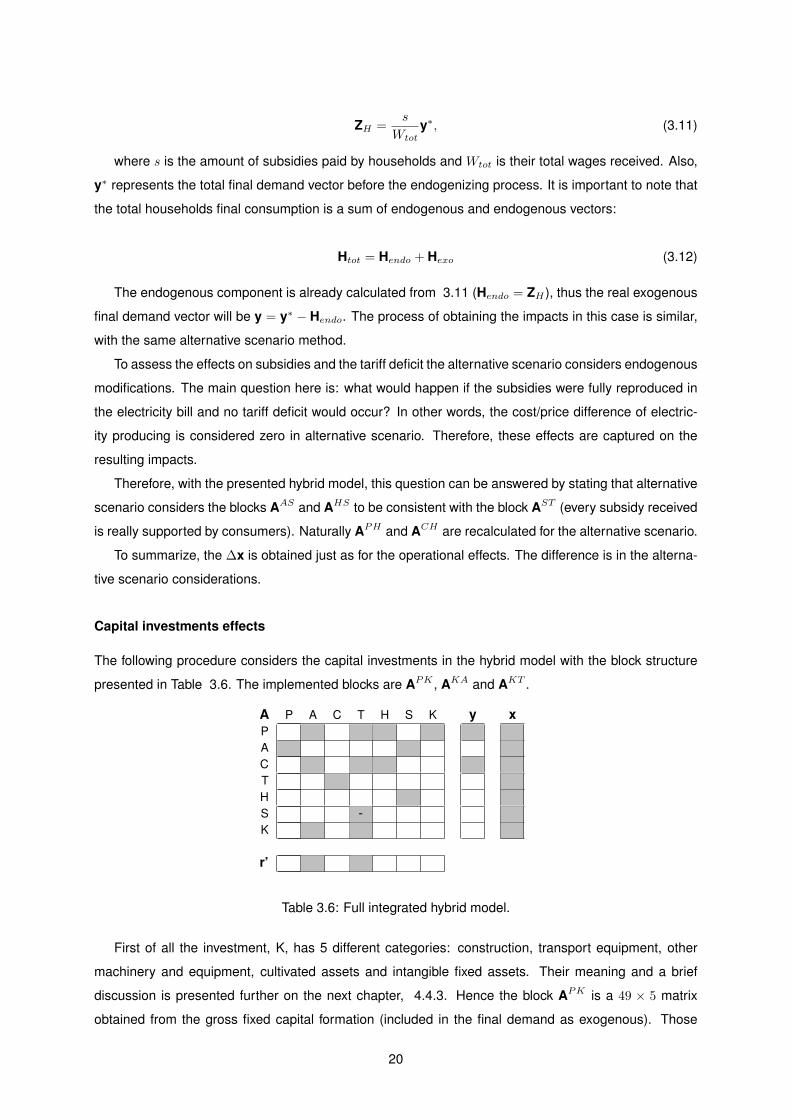
The following procedure considers the capital investments in the hybrid model with the block structure
presented in Table 3.6. The implemented blocks are APK , AKA and AKT .
A P A C T H S K y xPACTHS -K
r’
Table 3.6: Full integrated hybrid model.
First of all the investment, K, has 5 different categories: construction, transport equipment, other
machinery and equipment, cultivated assets and intangible fixed assets. Their meaning and a brief
discussion is presented further on the next chapter, 4.4.3. Hence the block APK is a 49 × 5 matrix
obtained from the gross fixed capital formation (included in the final demand as exogenous). Those
20
Page 41
values had to become endogenous according to a conversion key to disaggregate the 49 goods in those
5 categories. Obviously, just as the previous case with the endogenous households, the gross fixed
capital formation is removed from the final the demand as it is already considered inside the A matrix.
The AKA block is simply the consumption of fixed capital distributed across the 49 activities (without
counting the energy sectors: electricity and oil refining). However, the AKT block is more subtle. It
has to consider the investment expenditures related to the maintenance according to the consumption
of fixed capital. The investment portion related to the installation of new capacity power has to be
exogenous in order to contribute to the alternative scenario. The data manipulation to obtain this blocks
in detail is explained in the following chapter.
To sum, the reference scenario is obtained simply by xR = LRyR while the alternative scenario
includes a different approach:
xA = LRyA (3.13)
In this case the alternative scenario does not use the reference year final demand but a different
exogenous stimulus instead, yA. This alternative final demand vector does not include the investment
estimated to contribute to the installation of new capacity power (as it is considered only in the reference
final demand). Therefore, this analysis is possible for all of the 10 years, once the variable in this
alternative scenario is related to the exogenous stimulus and no previous year data is necessary. The
investment effects are thus isolated from every other effects.
21
Page 43
Chapter 4
Data and Assumptions
4.1 Overview and aggregation/disaggregation
The data gathering process is usually an intense and demanding step, because obviously it is intended
to find the most detailed and accurate data available. This is true for any study and/or research. In
the present work, this is no exception. The historical analysis requires a lot of different data sources to
interpret, cross information, evaluate compatibilities and apply some assumptions. To summarize, the
transition from raw to processed data (in the finished state) can be quite detailed and full of assumptions
that may need to be explained. This chapter 4 is dedicated to this mentioned process.
Detailed information has already been provided in the previous chapter, however, the fundamental
characteristics that should be retained before continuing are presented in the Table 4.1.
Model characteristics
Products 49Activities 49Technologies 18Carriers 42Final demand 5
Table 4.1: The model overview characteristics.
The model has 49 products and activities, 18 technologies (12 for generating electricity) and 42
carriers. The final demand has 5 components either for energy and economy. For economy it contains:
households; NPISH; government; GCF and exports. For energy the final demand includes: residential;
intermediate consumption (Rest of the Economy); stock variation; corrections and exports.
Sometimes the information required is available for n sectors or products while the goal should be
having it according to a classification of m sectors. The aggregation and disaggregation manipulating
methods provide the possibility to do the conversion of the desired information from n to m. If n > m, an
aggregation is what is required, thus the direction is towards a lower level of detail. However, if n < m a
disaggregation process has to be applied. Both these methods were used numerous times, hence it is
useful to briefly explain them in this introductory subsection for further reference.
23
Page 44
To start with, lets consider an aggregation. The first step is to establish the relation between the n
and m elements and build a bridge matrix (conversion matrix with 1’s and 0’s) that contains the identified
relation. For further use, lets call it the P matrix. Therefore, to aggregate is only necessary to multiply
the initial object by P. As an example, suppose M10×65 and it is intended to achieve a 10 rows and 49
columns matrix, M10×49. Here our n = 65 and m = 49. The aggregation would simply be:
M10×49 = M10×65P65×49 (4.1)
Disaggregation is more subtle, because it is about a conversion towards more detail. One can choose
do allocate the information equally (if one sector with data x is disaggregated into 3 other, each one of
them would have x/3). Regardless, this option is not very accurate and it can be misleading. What is
indeed required is called a proxy vector, v, to estimate a more accurate proportion. This vector has to
have the number of elements equal to m and it can be the output of those sectors, employment, capital
or whatever seems suitable. Consider P∗ to be the new bridge matrix with the new proportions and totj
the column j sum of the matrix resulting from diag(v)P. Each entry of the new proportional bridge matrix
is obtained as follows:
P ∗ij =
vjPij
totj(4.2)
Afterwards the process is similar to the aggregation method. The multiplication of the new proportions
matrix, P∗, by the object intended to be converted results in the desired dimension object.
4.2 Rest of the economy
The economy data gather is the most accessible part of the whole process. This is because there is data
in SUT format available for Portugal on the Eurostat database, for instance. Consequently, and consid-
ering our 2000 to 2010 year period, there was a change in the sectoral scheme from the years following
2006. In this case, from 1995 to 2006 the data was presented according to the Statistical Classification
of Economic Activities in the European Community (NACE), version 1.1 (59 sectors) and the following
years under the NACE 2 (65 sectors) conditions. The economic data was therefore arranged according
to this criteria and it was processed and modified to be a set of supply and use tables with 49 products
and activities 1. However, the GHG emissions were not included in the tables, although Eurostat also
contained this type of data by country and activities (following the same classification of NACE 1.1 and
NACE 2). For environmental concerns the emissions considered cover GHG such as carbon dioxide
(CO2), methane (CH4) and nitrous oxide (N2O). This data was further adapted to the 49 products and
sectors format using an appropriate conversion matrix. In this case both processes (59 and 65 to 49
sectors) were aggregations. Hence, the resulting vector containing the emissions was obtained accord-
ing to the aggregation method described above in which P is a 49 × 59 or 49 × 65 depending on the
1This processed version was given to me, and as mention in the acknowledgments, i have to thank Zeus Guevara and JoaoRodrigues for this data.
24
Page 45
conversion process to be before or after 2006. This operation is thus repeated for each one of the 10
years from 2000 to 2010.
Employment data was found on tables supplied by INE (available online). Although the information
was organized for 38 activity sectors, a equivalence key had to be constructed to disaggregate the data
into the 49 sectors. This was accomplished with proportional allocation (using Eurostat employment
proportions available from 2002 to 2010). The proportions from 2002 were assumed to be the same for
2001 and 2000 due to the lack of other accurate options. The disaggregation process was performed ac-
cording to the explanation provided in the previous section 4.1 where vt is the proxy used (employment
from eurostat relative to year t). In the end, the employment data for the 49 economic activities from
2000 to 2010 was processed and ready to be used. In addition, data for the fixed capital formation (in-
vestment) was required. This type of data is available from INE, (Statistics Portugal, National Accounts)
for 38 economy sectors. Therefore the equivalence key from 38 to 49 sectors was used and an identical
process as the one described above was conducted for each year (using economic output as proxy, v).
4.3 Characterization of the energy sector
It is within this sub chapter that the most important and significant part of the data gathering and as-
sumptions are made. This results from the disaggregation goal where more detail and information are
required. It is known that nowadays the energy sector plays a crucial role in society and in economy.
Considering this, and Portugal being a country mostly dependent on fossil fuel imports to meet the
energy demands, there has been an overall recognition that renewable have a significant developing po-
tential (NREAP 2010). As a result, the importance associated with this green sources is clearly known
mainly regarding electricity production.
4.3.1 Installed capacity and technology
To begin with, it was necessary to investigate the main technologies that would be responsible for the
electricity produced not only in Portugal mainland but also in the islands. The main division would be
to separate what is renewable and what are the conventional technologies. Sources as wind, solar,
hydro, biomass, waste and geothermal were first considered. In the following research steps fossil fuel
technologies, mostly thermoelectric were noted. Provided that, in Table 4.2 it is possible to see the main
electricity producing technologies considered for further analysis.
To explain these choices, a brief overview will be presented. Biomass dedicated includes power
plants that use wood and vegetal as well as animal waste. Those are facilities designed to produce
electricity by burning biomass residues. On the other hand, some plants may allow combined cycle
biomass (CHP), and that represents increased efficiencies in the whole process due to the re-use of the
released heat in the combustion cycle. Although the fuel is the same in principle, several differences
were identified, and the cost structure was no exception, as it will be discussed later on. Some doc-
uments present also this separation, as for instance yearly reports on DGEG database (DGEG 2013).
25
Page 46
Energy Technologies
Biomass DedicatedCHP
MUW Incineration
Biogas
Wind On-shore
Hydro SmallLarge
Geothermal Binary Cycle
Solar Photovoltaic
ThermoelectricFuel Oil (CCOT)Coal (PCC)Natural Gas (CCGT)
Table 4.2: Electricity generation technologies. Combined Heat and Power (CHP) allows heat supply aswell.
Similarly, municipal solid waste based on mostly the incineration of industrial residues also contributes
to electricity production in Portugal, even though as a smaller fraction. The use of biogas, is an emerging
technology since there are still goals that need to be achieved in our established road maps. In fact, the
main application of biogas is for electricity production (Miguel Ferreira & Malico 2012).
The potential in wind power is widely accepted and its continuous growth has been notorious over
the years (INEGI 2010). Additionally hydro power can be divided in two different categories: small scale
and large scale. This distinction is widely accepted in the 10MW capacity mark, i.e. small scale refers to
facilities with power capacity below 10MW and large scale is for the remaining plants with more than that.
This separate technology consideration within hydro power is important because i) the investment and
Operation and Maintenance (O&M) costs are not the same and they change significantly; ii) electricity
is produced under two different regimes, in which small scale hydro is a part of the SR and large scale
is considered as OR resulting in different policies, incentives and subsidies (discussed in more detailed
further).
Usually one of the greatest differences about consider just Portugal mainland or decide to include the
islands is connected with geothermal power. The possibility of producing electricity from this renewable
source depends on the region, due to geological properties. In particular, Azores is the only Portuguese
region where this is possible and, in fact, in S. Miguel this source meets about 40% of the population’s
electricity requirements (Alison Holm & Gawell 2010). For this reason Geothermal was included in the
characterization using a binary cycle conversion to produce electricity due to the working conditions
of these power plants (Ribeira Grande and Pico Vermelho). Another technology considered, and the
last renewable source is Solar Photovoltaics (PV). Portugal once had the biggest photovoltaic power
plant in the world (Moura, Amareleja power station) and the electricity produced from solar sources has
been growing in the recent years, making this inclusion in the characterization one mandatory choice.
To finish the electricity (and heat) producing technologies, the thermoelectric sector was added. It is
important to note that cogeneration (non-renewable CHP in this case) is included as a part of fuel oil
26
Page 47
and natural gas technologies. In the description Table 4.2, Combined Cycle Oil-Turbine (CCOT) and
Combined Cycle Gas-Turbine (CCGT) exposes the assumption that was made. To put it in another way,
after some research on these fossil fuel plants, it was observed that most thermoelectric systems do
work according to this cycles and assuming the costs (O&M and investment) associated with this type of
power stations is an accurate assumption. As for coal, Pulverized Coal Combustion (PCC) is the most
common cycle implemented in these coal power plants. To illustrate the evolution of each one of the
described technologies in Portugal, the Figures 4.1 and 4.2 are displayed in MW.
0
500
1000
1500
2000
2500
3000
3500
4000
4500
5000
2000 2001 2002 2003 2004 2005 2006 2007 2008 2009 2010
MW
Wind
SmallMhydro
LargeMHydro
Photovoltais
Geothermal
BiomassMdedicated
BiomassMCHP
MSW
Biogas
Figure 4.1: Evolution of the accumulated power capacities for each renewable energy technology con-sidered.
0
500
1000
1500
2000
2500
3000
3500
4000
4500
2000 2001 2002 2003 2004 2005 2006 2007 2008 2009 2010
MW
Coal
Fuel oil
Nat. Gas
Figure 4.2: Evolution of the accumulated power capacities for each conventional fossil fuel technologiesconsidered.
Over the 10 years period from 2000 to 2010 several power plants were built, some were improved
with new groups (more capacity) installation, others became non operational. The challenge is to dis-
cover the facilities profile, in the most accessible way possible, and create a database with information
such as the accumulated capacity installed and electricity produced over the years for each technology
described above. To obtain these values several sources were consulted, although the main database
was DGEG with yearly reports and tables available online. At the same time, some information was rela-
tive only to Portugal mainland, thus it was necessary to compare different documents (including Madeira
and Azores) to extract the desired information. After obtaining it, the evolution share was calculated
27
Page 48
summing the renewable electricity produced from all RES technologies versus the fossil fuel thermo-
electric contribution. The result is illustrated in Figure 4.3. The RES-E significant growth over the years
becomes clear, reaching over 50% in 2010. RES‐E Non RES‐E
0,0
10,0
20,0
30,0
40,0
50,0
60,0
70,0
80,0
90,0
100,0
2000 2001 2002 2003 2004 2005 2006 2007 2008 2009 2010
Historical electricty share
RES‐E Non RES‐E
Figure 4.3: Evolution of the electricity production share percentage by renewable sources vs. nonrenewable (fossil fuel).
4.3.2 Investment and O&M costs
Additionally, information on investment, operation and maintenance costs were also required. In order
to accomplish these costs and obtain a reference value for the selected technologies, the main sources
were EU (2008), Kaplan (2008), EIA (2013), NREL (2012), IEA & NEA (2010), among others. The costs
presented in each document seem to slightly change because they are very dependent on region, type
of plant, location, and several other characteristics of the project. Despite that, the values presented
in the Table 4.3 are reference costs chosen considering several documentation such as the citations
above.
The asymmetric tolerance ranges for investment costs are also presented. These were accomplished
by consulting several documents that had different values for investment (and different ranges). For
both O&M values no fixed range was obtained due to the nature of these costs (extremely dependent),
although the margins must be in average around the order of 10 to 20%. However, the reference values
were used and no statistical error analysis was conducted during this procedure (a further step adjusts
the absolute values to match the national accounts numbers on capital formation).
These values were prepared and had to converted in the same monetary unit (same reference year).
The investment costs are considered to be overnight costs, i.e. the power plant/station would require
that amount of money per capacity installed if it would be built overnight. Fixed O&M costs are expenses
fixed, hence do not change (at least significantly) from power plant to power plant. On the other hand,
the variable costs do, and they are dependent on the amount of electricity produced. It is important
to mention that both these operational and maintenance costs do not include fuel expenses (which
is of great importance for the thermoelectric technologies). However, this is actually not problematic,
28
Page 49
Technology Investment [e2005/kW] Fixed O&M [e2005/kW-yr] Variable O&M [e2005/MWh]
Biomass Dedicated 2400+770−430 67 10
Biomass CHP 5900+885−885 226 11
MUW 6200+930−930 250 5
Biogas 3140+2650−180 245*
Wind on-shore 1140+230−140 19 -
Small Hydro 3500+1300−1000 17 -
Large Hydro 1800+1300−450 8 -
Solar PV 4700+2200−600 13 -
Geothermal 3500+1500−1500 56 7
Fuel oil 900+200−350 45*
Coal 1265+175−265 60*
Natural Gas 635+95−155 25*
Table 4.3: Costs structure considered for each technology. The marked numbers (*) consider bothvariable and fixed O&M due to their different sources.
because the use of carriers by technologies is represented in energy units and therefore no double
counting occurs.
In order to asses the investment costs, the accumulated capacities were consulted (from the database
created with the available data) and from the installed capacities it would be assumed that for each kW
increase from one year to another the investment would be the price presented in Table 4.3. If there
was no capacity installation it is assumed that no investment occurred. Altogether, this assumption is
acceptable due to the constant power plants installation in technologies such as wind energy. From the
period 2000 to 2010 the conventional thermo power plants were considered individually because Natural
Gas was the only technology growing with several stations becoming operational over these years (see
Table 4.4). Therefore, it can be seen the reason why it was considered no investment took place from
2000 to 2010 in technologies as coal and fuel oil power plants. Furthermore, it is possible to compute ta-
bles with information referring to year by year monetary expenditures on investment (Gross fixed capital
formation) and by operating and maintaining every power station of each technology.
4.3.3 GHG emissions and employment
In general there are three ways for estimating the green house gas emissions: i) fuel-specific emission
factor coefficients; ii) direct measurement; iii) mass or carbon balance approach (Herold 2003). For
estimating the emissions of CO2, CH4 and N2O by each one of the technologies considered the first
method is selected. The data was gathered from IPCC 2006 Guidelines (Gomez et al. 2006) and the
coefficients are presented in Table 4.5. Note that the coefficients in the category ”Solid Biomass” were
also used for the combined cycle technology (assumed to be similar). As a result, knowing already
the electricity produced from each source and considering the efficiency in converting fuel (input) to
29
Page 50
Power Plant Cap.[MW] Year
Gas NaturalTapada do Outeiro II 990 1999 - PresentSOPORGEN 67 2000 - PresentENERGIN 43 2002 - PresentRibatejo 1176 2004 - PresentLares 826 2009 - PresentPego II 837 2010 - PresentFISIGEN 25 2010 - Present
Fuel OilCarregado 708 1969 - 2009,2010,2011*Tunes 165 1973-2010 - PresentSetubal 946 1979 - 2012Barreiro 64,5 1979 - 2009Central Termoelectrica de Porto Santo 19 1992 - Present
CoalSines 1180 1985-PresentTapada do Outeiro I 150 1959-2004Pego I 576 1993 - Present
Table 4.4: Thermoelectric power plants in Portugal and their capacities. The symbol (*) is intended tonote that in each year a facility group of 236 MW was closed.
electricity the GHG emissions in physical units (Tonnes) were calculated for the energy sector.
Technology/Fuel CO2 CH4 N2OMin Ref Max Min Ref Max Min Ref Max
Hard coal 95.00 100.00 105 0.30 1.00 3.00 0.50 1.50 5.00Crude oil 71.10 73.33 75.5 1.00 3.00 10.00 0.20 0.60 2.00Natural gas 54.30 56.10 58.3 0.30 1.00 3.00 0.03 0.10 0.30Solid biomass 66.00 80.70 100 10.00 30.00 100.00 1.50 4.00 15.00Biogas 46.20 54.60 66 0.30 1.00 3.00 0.03 0.10 0.30MSW 73.30 91.70 121 10.00 30.00 100.00 1.50 4.00 15.00
Table 4.5: GHG emission factors used per fuel-type/technology in tonnes per TJ of input (Gomez et al.2006).
Due to several policies and protocols already mention in early chapters, such as Kyoto, there has
been an obligation referring to CO2 emissions. Usually this results in another cost for the electricity
producers, which is the carbon emission tax price (e/Ton). In 2005 European Union Emission Trading
Scheme (EU ETS) was implemented targeting the reduction of GHG emissions. These values are
presented in Table 4.6 in current prices. Consequently, these emission costs can also be considered in
the further analysis as they were not included in the previous O&M expenditures mentioned. Therefore,
avoiding several amounts of carbon dioxide emissions can also be seen as avoiding money expenditures
on CO2 allowances. This could encourage the efforts to reduce the carbon emissions by electricity
producers in addition to the proclaimed environmental concerns.
In order to simplify the results display in the following chapter 5, the methane and nitrous oxide emis-
sions can be presented in carbon equivalent emissions. To accomplish this, Global Warming Potential
(GWP) is a relative measure that can be used. It measures the amount of heat a certain GHG traps in
30
Page 51
CO2 price 2005 2006 2007 2008 2009 2010
e/ton 21 17 1 18 13 14
Table 4.6: Carbon emission prices in current e/ton. From Reinaud (2007).
the atmosphere in comparison to the amount trapped by a similar mass of carbon dioxide. Hence, the
GWP for methane over 100 years is 25 and for nitrous oxide 298. In other words, it means that emissions
of 1 million metric tonnes of methane and nitrous oxide respectively is equivalent to emissions of 25 and
298 million metric tonnes of carbon dioxide (Forster et al. 2007).
Another key point is green jobs. They are still controversial, because although jobs can be created by
the renewable they could be destroyed elsewhere. Hence, one of the most important question is about
employment. So, in a similar way, data had to be found for each of these technologies that were chosen.
Direct jobs are related with the primary industry sector and include jobs in fuel production, manufactur-
ing, construction and O&M (Rutovitz & Harris 2012). For this model purpose the data required is just
for fuel handling (fossil fuel technologies) and O&M and it is described with detail in Rutovitz & Harris
(2012). This is because construction and manufacturing jobs will be described on the rest of the econ-
omy and therefore associated with each technology by the hybrid model built presented in the previous
chapter. The extracted data is presented in the Table 4.7.
Technology O&M [Jobs/MW] Fuel [jobs/PJ]
Dedicated Biomass 1.5 32.0Biomass CC 2.3 32.0MSW 1.5 32.0Biogas 1.5 32.0Wind 0.2 0.0Small hydro 2.4 0.0Large Hydro 0.3 0.0PV 0.3 0.0Geothermal 0.4 0.0Oil 0.1 22.0Coal 0.1 40.0Natural Gas 0.1 22.0
Table 4.7: Job creation data for each technology. From Rutovitz & Harris (2012).
4.3.4 Electricity subsidies, tarriffs and the tariff deficit
The special regime production, which includes cogeneration and renewable sources other than large
hydro plants, supplies power to REN under special ”Feed-in” tariffs decided by the government (Amorim
et al. 2013). In Table 4.8 these prices guaranteed to the special regime producers are presented and
in Figure 4.4 the graphical representation is displayed. No geothermal data was found, meaning that no
substantial subsidy is associated with this technology (assumption). ”Feed-in” tariffs have already been
discussed in previous chapters but now it is possible to have an idea of their values really received by
the producers per MWh of electricity generated.
31
Page 52
Technology 2000 2001 2002 2003 2004 2005 2006 2007 2008 2009 2010
RES CHP 44.00 47.75 55.50 80.00 81.00 79.00 82.00 86.00 91.00 90.00 90.50Other CHP 48.00 56.50 67.00 77.00 79.75 92.00 103.00 100.00 122.00 99.00 104.50Wind on 60.25 62.00 80.00 84.50 88.00 89.50 92.25 95.00 95.00 94.50 92.00Small hydro 54.50 65.50 75.75 78.75 80.00 82.00 84.75 89.00 89.00 88.00 89.00MSW 56.00 66.00 69.00 71.00 73.00 75.00 77.50 79.00 81.00 80.00 80.00Biomass 60.00 64.50 67.00 69.50 72.75 102.50 111.50 110.50 112.00 110.00 109.00Biogas 54.00 55.25 45.00 53.00 69.75 95.75 106.50 105.00 109.50 106.50 108.00Solar PV 0.00 0.00 0.00 520.00 522.50 520.00 380.00 330.00 337.50 302.50 305.00
Table 4.8: SR subsidies. ”Feed-in” tarrifs values in current prices [e/MWh] from 2000 to 2010 (Amorimet al. 2013).
The graphic representation of Table 4.8 is shown in Figure 4.4. The secondary axis, in the right
hand-side, is related to photovoltaic technologies (much higher than the ones for other technologies).
0
100
200
300
400
500
600
0
20
40
60
80
100
120
140
2000 2001 2002 2003 2004 2005 2006 2007 2008 2009 2010
€/M
Wh
Special Regime Subsidies ‐ FiTs
OtherMCHP
RESMCHP
WindMon
SmallMhydro
MSW
Biomass
Biogas
Solar
Figure 4.4: Special Regime. ”Feed-in” tarrifs values in current prices [e/MWh] from 2000 to 2010. Datafrom Amorim et al. (2013).
As it was mentioned before, the ordinary regime production, benefits from their own incentives, usu-
ally known as CMEC/PPA. They exist to support the investment costs of conventional thermo plants and
large hydro power power plants, and their average value per year is displayed in Table 4.9. The sub-
sidized OR production plants ratio was also applied to total MWh per technology to obtain the absolute
amount spent per year.
OR 2000 2001 2002 2003 2004 2005 2006 2007 2008 2009 2010
PPA/CMEC 48.4 48.0 52.2 46.0 55.9 67.7 59.1 67.8 97.9 73.7 62.1
Table 4.9: Ordinary Regime. Power Purchase Agreements (PPA) / CMEC values in current prices from2000 to 2010 (Amorim et al. 2013).
When observing the electricity bill, the price mentioned is not only due to the energy price acquired.
To explain, it contains three main components: the energy itself; grid connection tariffs and Custos de
Interesse Economico Geral (CIEG) (ERSE 2013). These shares are not constant over the several types
32
Page 53
of consumer. In fact, these CIEG contain other sub-divisions such as SR and OR production subsidies
expenses (at least part of them), other rents, among other components that differ from high voltage
consumer to a low voltage consumer (Abreu 2012). In Portugal, the responsible entities mention these
consumers in the literature as follows: Baixa Tensao (BT), Media Tensao (MT), Alta Tensao (AT) and
Muito Alta Tensao (MAT). See Table 4.10 for the detailed share values used. The BT is usually divided
into more detailed categories, and as a result the average of Baixa Tensao Normal (BTN) and Baixa
Tensao Especial (BTE) is expressed as BT to simplify the calculations.
Electricity bill components BT AT MT MAT
Energy 0.47 0.67 0.60 0.73Grid 0.28 0.15 0.23 0.08CIEGMunicipal Rents 0.06 0.00 0.00 0.00Costs SR 0.05 0.07 0.06 0.07Costs Autonomous Regions 0.04 0.02 0.03 0.00Costs OR (CMECS/PPA) 0.08 0.06 0.06 0.08Other 0.02 0.03 0.02 0.03
Table 4.10: Electricity costs decomposition [%]. Data from ERSE (2013).
These type of data (structural decomposition of the bill components) is very detailed and, was found
for 2 years. Therefore, it was assumed they remained constant from 2000 to 2010. According to the type
of customer it was estimated what was paid from each of the economic sectors including households.
From DGEG, it can be extracted, for this year range, data about the electricity consumed per activity
sector and depending on whether it is a low or high voltage consumer. The proportions were estimated
from this raw data tables. Hence, this proportions were applied to the historical use of electricity (in
GWh) per type of voltage customer. Moreover, the electricity prices over the years are displayed in Table
4.11.
e/MWh 2000 2001 2002 2003 2004 2005 2006 2007 2008 2009 2010
MAT 42.30 43.08 41.60 42.10 44.30 48.73 50.13 53.28 55.00 57.70 58.60AT 46.34 47.20 43.59 44.20 45.80 50.92 52.74 56.57 58.80 62.30 64.40MT 64.52 65.54 64.41 65.60 67.50 73.36 77.67 81.43 84.10 89.40 92.25BT 114.05 115.50 108.59 111.60 113.90 116.64 120.22 131.76 137.45 144.30 148.90
Table 4.11: Electricity prices evolution per type of consumer. Data source from DGEG.
The total amount paid by each activity sector was thus estimated. Then, using the costs share
decomposition in Table 4.10 the amount of subsidies paid for the SR production was simply obtained.
Note that the unprocessed activity sectors were 28 until 2007, 78 in 2008, 88 in 2009 and 85 in 2010.
As a result, several conversion matrices, P, had to be constructed from specific aggregation keys. The
resulting data can be consulted in the appendix section.
Within this time period from 2000 to 2010, several things have changed in the energy sector, specially
in the electricity area such as the transition to the ”free market” and the inclusion of several renewable
sources. Since 2006 and especially in 2008 with the substantial increase of fossil fuel prices the average
costs of electricity followed that behavior (BPI 2011). Despite that, the Portuguese Government wanted
33
Page 54
to keep electricity and energy in general at a rather low price (comparable to the real costs). The
producers costs were paid the full amount of these subsidies (because only a part of it was really paid
by the consumers) by EDP Servico Universal and REN. These entities supported these costs, while the
ordinary customer was charged less than it should be (ERSE had the prices regulated so that producers
could not charge more than the established price). Under those circumstances, the debt started to
increase, and is commonly known as tariff deficit in the energy sector. To summarize, this debt will be
paid in the following years, with interests, once the charged prices did not follow the real production,
transportation and distribution costs. It is a rather controversial issue, and some argue that this deficit
should be eliminated as fast as possible recurring to a loan with low interest rate (GEOTA 2013).
4.4 Energy and ROE interaction
The present section is dedicated to the explanation of the data gathering process and assumptions
connected to both energy and economy. The main goals here were to build the use of economic products
by technologies and the use of energy carriers by activities in the economy.
4.4.1 Use of products by technologies
To start with, let’s consider first the use of products by energy technologies. Although several documents
were consulted, not many information seemed to be available with the expected detail. Usually this type
of information could be gathered with more detail using specific surveys on a sample of power plant
facilities for each technology proposed. As this was very unlikely to succeed (not public information),
similarly data was found from Oliveira et al. (2013) and rearranged, thus obtaining the O&M costs share
presented in Table 4.12.
O&M costs share [%] Hydro Biomass Wind PV Geothermal Non RES-E
Real estate services 16.2 1.5 9.8 8.6 1.7 15.2Financial servies 6.5 0.5 6.1 23.0 16.7 12.9Telecommunications services 1.3 13.4 2.0 0.6 0.0 7.0Accommodation and food services 0.0 15.1 2.5 0.0 0.0 2.3Transport services 1.3 15.1 2.0 0.6 0.0 1.2Trade services 3.2 13.4 2.0 2.9 0.0 2.9Constructions 26.0 0.8 6.1 9.2 8.3 11.1Waste collection 0.0 16.8 0.0 0.0 0.0 0.0Water treatment 3.2 13.4 2.0 2.9 8.3 0.0Machinery and equipment 12.3 2.3 8.2 11.5 15.0 10.5Electrical equipment 12.3 2.3 8.2 10.9 16.7 10.5Fabricated metal products 11.7 2.8 8.2 11.5 16.7 8.8Basic metals 2.6 1.7 9.8 15.5 16.7 14.6Rubber and plastics products 3.2 0.8 32.8 2.9 0.0 2.9
Table 4.12: Use of economic products by the energy technologies. From Oliveira et al. (2013).
First of all, the technology description does not match the one discussed before. With this in mind,
some data had to be used for more than one technology. To explain, for example, hydro products use
34
Page 55
share is considered the same for small and large scale plants, biomass data is used not only for biomass
dedicated and CHP but also for biogas and waste. Moreover, NRES-E data is equally applied to fossil
fuel plants. The next step is based on the calculation of the absolute values of O&M per year for each
technology and allocate them according to this data. After establishing a key relating these products
to the 49 of Eurostat, the tables were computed and adjusted to match the national accounts on the
economic model. To explain, the normalized conversion matrix 49× 14 , P∗, was calculated according to
disaggregation method described in section 4.1. The vector vt (year t) is the use of the 49 products by
the ”Electricity and gas” sector and it is used as a proxy to perform proportional allocation. Under these
circumstances, the matrix Mt is obtained using the following expression:
Mt = P∗T diag(ct) (4.3)
These process is similar to the one described earlier for employment and it is has numerous appli-
cations throughout the whole data manipulation required for this work. The T matrix contains the O&M
share values presented in Table 4.12, while ct is the absolute O&M values in year t (calculated from
the costs gathered and installed capacities in Portugal). In order to have these resulting matrix, Mt,
matching with the economy values for the electricity sector, this matrix was adjusted. In addiction, the
remaining portion of these costs were allocated to another sector ”other”. Then, these remaining costs
in ”other” were disaggregated using proportional allocation (considering energy output as proxy) to the
technologies: natural gas distributed and electric grid. On the other hand, the ”Manufacture of coke,
refined petroleum products and nuclear fuels” (”Oil Refining” in short: see appendix A.4 for the clas-
sification list) use of products was identically distributed proportionally to the following technologies: oil
refinery, coal refinery, biodiesel and petrochemical. To ensure that this distribution criteria is valid INE
(2007) was consulted. To summarize, the final matrix, is a 49× 18 in monetary units containing the use
of products for each one of the 12 electricity generation technologies plus these 6 other technologies to
close the energy sector.
The total expenditure by energy technologies on economic products, in constant prices of 2002, is
shown in Figure 4.5.
These values do not include the use of energy products in monetary units ( products number 10 and
22: see Table A.3 in the appendix section). The growth of the total use reaches the maximum value of
5193 Me2002 in 2007. Since that year, these values get reduced revealing themselves as, perhaps, an
indicator for the crisis period.
4.4.2 Use of carriers by activities
The economic activities also use energy carriers. Therefore, this information also has to be included so
that the economy, energy and their interaction is described in the most accurate way possible. There
were 2 different reliable sources where this information could be found, one from INE and the other from
DGEG. The first only had 14 carriers for the 50 sectors required (49 activities plus households after
aggregation) and DGEG data had the 42 carriers required but for 24 activities. Although the raw data
35
Page 56
0
1000
2000
3000
4000
5000
6000
2000 2001 2002 2003 2004 2005 2006 2007 2008 2009 2010
TotalMexpenditureMonMproductsMbyMtechnologiesM[M€]
Figure 4.5: Use of economy products by technologies (except energy related) in Me2002 by year.
seemed to be available, the need for manipulation (e.g. establishing aggregation and disaggregation
keys with proportional allocation) was obvious. That is to say, maintain the dimensions required, i.e. 49
activities and 42 carriers. The DGEG source was compatible with the energy SUT used. Therefore, one
of the restraints was the row sum (use of carriers) and the other restrain was column sum (total sector
use of carriers).
Hence, an initial matrix, Mi, had to be transformed into another matrix, Mn, according to the desired
row and column sum vectors, un and vn (Okuyama et al. 2002). This is the original RAS procedure or
bi proportional technique. In the end, after evaluating the resulting matrix, it respected the constraints
(although it is an iterative method and the the result is defined with a tolerance) but the original table
obtained with proportional allocation (42 × 49) from DGEG was more reliable to use than this manipu-
lated RAS one. Consequently the final matrix used was indeed the one obtained from DGEG after a
proportional desegregation process (total use of carriers per sector as a proxy vector from INE data).
4.4.3 Breakdown of investment costs
Investment costs were estimated according to the procedure mentioned earlier on the present chapter
(installed capacities times the costs in Table 4.3). However the absolute values are not enough. To put it
differently, these costs have to be assessed to economy activities, i.e. cost breakdown per activity. This
process can be divided in two steps: first, gather the data shares with the raw categories and secondly,
manipulate them so that they match our economic sectors division. To find these data several technical
reports from several institutions were consulted such as Krohn et al. (2012) for wind energy technology,
IRENA (2012) and EIA (2010b) for hydro power plants. In addition, geothermal power plant investment
information comes from document sources such as EIA (2010a) and Henneberger (2013). The remain-
ing technologies breakdown is provided with some detail in NREL (2012). All of these gathered data (in
an intermediary step of manipulation) is provided in Table 4.13.
In order to evaluate the investment for the 12 electricity technologies some shares were considered
36
Page 57
Investment share allocation [%] Biomass Wind Hydro PV Geothermal Coal Nat. Gas
Construction 0.26 0.13 0.40 0.07 0.79 0.61 0.58Transport equipment 0.02 0.04 0.02 0.04 0.01 0.01 0.01Other machinery and equipment 0.38 0.74 0.29 0.82 0.10 0.13 0.18Cultivated assets 0.00 0.00 0.00 0.00 0.00 0.00 0.00Intangible fixed assets 0.15 0.04 0.07 0.02 0.11 0.08 0.06Owners cost 0.19 0.05 0.23 0.05 0.00 0.17 0.17
Table 4.13: Most significant fractions of the investment costs breakdown structure per energy technology.
the same. To explain, biomass share was considered the same for biomass dedicated, biomass CHP,
MSW and biogas; hydro power share was equally used for large and small power plants; and fuel oil has
the same share as natural gas technology (literature assumption). Considering that T is the technology
investment share matrix (fixed over time) created from sources described above while the vector c is
the absolute values of investment for each technology in year t, the new investment matrix for the 12
electricity technologies is
Mt = PT diag(ct) (4.4)
The P matrix is used to aggregate 12 assets (NACE A10 plus transportation and owner’s costs)
into 6, and the matrix resulting from PT is displayed in Table 4.13. To summarize, the data was first
manipulated to match the 10 sector NACE division, A10, and further aggregated according to the de-
scribed process. Afterwards the resulting matrx was adjusted to match the values from the gross fixed
capital formation Tables (”Electricity, gas, steam and hot watter supply” sector) provided by the Statistics
Portugal, National Accounts (INE). In the end, the whole process is repeated for each year.
Although some categories are self explanatory it is preferred to briefly discuss them. To start with,
construction activities have the most share for geothermal technology. The injection wells and systems
for the pipelines and the construction of power plant itself justify this superior share of 79%. Trans-
portation material was assumed to be 5% of the allocated shares for ”Industry, energy, water supply
and sewerage” in the A10 classification. The following sector, ”other machinery and equipment”, also
contains specialized equipments such as boilers, turbines, steam engines, and so on. Hence, solar pho-
tovoltaics and wind energy have the two highest shares on this sector due to the turbines, basic metals
and the high capital requirement for solar panels (the modules and the structure). Cultivated assets are
not a significant portion of the capital investment, and therefore have no percentage share for each one
of the technologies. In fact this asset is only applied to agriculture, forestry and fishing. The” intangible
fixed assets” activity sector concern the financial and insurance activities, real estate activities, admin-
istrative and support service activities among others. However, owner’s cost definition may differ in the
literature. One of the possible definition states that these costs are related to the development, pre-
liminary feasibility and engineering studies, environmental studies and permitting, legal fees, insurance,
property taxes during construction, and the electrical interconnection (including transmission system)
(EIA 2013). Despite that, this category of costs is not considered in the further analysis.
To summarize, it was explained how the total investment by technology, category and year were
37
Page 58
estimated. Now, the detailed process on data manipulation to estimate the maintenance and capacity
power installation investment is presented. Recall the previous chapter where the investment costs are
added in the model, 3.2.3. Technology x has one specific vector Kxi containing the average proportions
for each investment category i:
Kxi =
2010∑t=2000
kit
5∑i=1
2010∑t=2000
kit
(4.5)
From each one of these vectors a proportions matrix (each column sum is 1) is obtained (technology
as columns and categories of investment as row).
Thus, to estimate the investment related to the maintenance, the proportions matrix is applied to the
consumption of fixed capital for each year. The resulting matrix is used as the endogenous block for
investment in technologies. Afterwards, the total investment matrix is subtracted from the investment re-
lated to maintenance. The resulting matrix is assumed to be the investment expenditure by category and
technology directly related to the installation of new capacity power. This is the exogenous investment
considered discussed previously in the method description.
The installed power on renewable energies and on other power plants (mainly natural gas) is more
significant on recent years. This fact is confirmed, as expected, in the historical evolution of both portions
of the investments. The total investment expenditure related to maintenance and associated to the
installed power is displayed in the Figure 4.6.
0
500
1000
1500
2000
2500
2000 2001 2002 2003 2004 2005 2006 2007 2008 2009 2010
Maintenance Installed Capacity
Figure 4.6: Total investment expenditure in the energy sector related to the maintenance and the in-stalled capacity in Me2002 by year.
The endogenous investment related to the maintenance is smaller and piratically constant over the
years which is understandable. The investment in constructing new power plants, wind farms, hydro
damns, etc as well as installing more capacity power is rather large, reaching its peak in 2009 with more
than 2000 Me2002 spent on the improvements of the energy sector.
38
Page 59
Chapter 5
Results
5.1 Scenarios and structure
Portugal, as many other worldwide countries, has been facing numerous modifications in the energy
sector over the years. In addition to the technologies mix development, subsidies to electricity producers
and capital investment also contribute to the overall structure as seen in chapter 3 . These modifications
are applied to what is understood as an integrated system of different axis interacting with each other
E3.
Therefore, it is considered three different effects. First the effect related to the energy sector devel-
opment year by year (technologies). Secondly, the effect resulting from the capital investment (towards
capacity installation) in the energy sector. The third one is related to the subsidies and tariff deficit, i.e.,
what would happen if the subsidies paid to the electricity producers were supported consumers (no debt
scenario where electricity costs are represented in its price). These three different effects combined
provide an answer to the Portuguese energy policy applied during this 10 years time line.
The economic, social and environmental impacts are calculated recurring to alternative scenarios.
These scenarios are built considering the different effects mentioned above. The first alternative sce-
nario considers that the energy sector remained constant from the previous year until the year studied
(same technology description). The second alternative scenario provides an alternative view to what
would have happened if no capital investment in the energy sector would occur. Thirdly, the alternative
scenario considers that no debt (tariff deficit) would occur once the subsidies are completely paid by
consumers in the same year.
This chapter structure is organized to be followed with increasingly more detail, i.e., results keep
getting more disaggregated. Hence, this chapter will start with general results and impacts of the Por-
tuguese energy policy (effect combination) in section 5.2. After, within this subsection, the net impacts
are presented for the energy sector and the rest of economy (ROE) considering different types of im-
pacts. The final section 5.3 intends to disaggregate the results by type of effect, and within each
subsection (each for effect), the results are displayed for every economic activity and each energy tech-
nology.
39
Page 60
The economy model consists in 49 activities and products. Hence, to ensure an easily understand-
able display of results those activities were converted to a system of 10 (A10 classification). After the
”raw” results were obtained the aggregation process was applied and the results can be presented ac-
cording to the description provided in the appendix section, Table A.5.The results for the energy sector
are shown for 14 technologies. Besides the 12 electricity producing technologies (Table 4.2), there is
oil refining as number 13 and the residual one is called as ”other”. This final category is an aggrega-
tion of the remaining 5 technologies (coal refining, natural gas distributed, electric grid, biodiesel and
petrochemical - see A.1) due to their relevance assumed in this work.
5.2 Total impacts
In this section the total impacts are presented. First, the overall results are displayed for each type of
impact. Afterwards, the total separated impacts disaggregated only by effect, i.e, operational, capital
investment and subsidies/tariff deficit are shown. The Table 5.1 shows the observed absolute impacts
in the reference scenario. The purpose of this table is to provide an insight about the Portuguese reality
GVA [Me2002] Employment [103] CO2eq [Mton]Year Energy ROE Energy ROE Energy ROE
2000 2383 65475 18 5559 22 542001 2504 114423 17 5620 22 532002 2606 115141 15 5658 26 542003 2807 114382 15 5631 21 532004 2884 116241 14 5623 23 542005 2759 117148 13 5619 26 542006 3018 118649 13 5622 23 522007 3117 126920 13 5692 21 502008 3423 127144 12 5707 20 492009 3002 144086 12 5561 20 442010 3456 147049 11 5464 15 44
Table 5.1: Reference scenario impacts for each year and impact type.
regarding both energy and economy between 2000 and 2010.
5.2.1 Overall
The most general and fundamental question that motivated this thesis work is related the evaluation of
the impacts of Portuguese energy policy. Combining the considered effects, the results (in the most
aggregated way possible) that provide an answer to this formulated question are presented in Table 5.2.
The economic impacts studied are related to the GVA which is proportional to the GDP and this is
a key indicator of the country whole economy condition. From observing the table, the national energy
policy generated economic output until 2009. Afterwards, these policies costed 278.02 Me2002. However
note that comparing to the absolute values in Table 5.1, these impacts represent less than 1%. The
social impacts follow the same behavior, generating employment mainly due to investments associated
40
Page 61
Year GVA[Me2002] Employment [103] CO2eq [Mton]
2000 125.45 12.76 0.182001 579.04 26.06 -0.362002 81.80 2.37 1.852003 123.08 10.00 -2.762004 223.66 10.37 1.052005 395.77 19.31 0.772006 320.36 22.62 -1.632007 973.96 42.90 -1.262008 599.33 28.52 -0.072009 39.15 13.35 0.122010 -278.02 -0.82 -4.60
Table 5.2: Total impacts of the Portuguese energy policy.
with capacity installations (as it will be clarified in the following subsections). In 2010 the total result
accounts for the loss of 820 jobs. Although in 2010 the impacts start to be negative for economy and
employment, the environmental impacts show that the future seems to be ”greener’. In fact 6 out of 10
analyzed years show a cleaner environment, culminating in 4.60 Mton of GHG avoided emissions into
the atmosphere.
The following subsections will disaggregate the Table 5.2 by effect for economic, social and environ-
mental impacts.
5.2.2 Economic impacts
In Table 5.3 the net contribution of each effect regarding the economic impacts is shown. Note that
in the operational analysis (model with O&M costs) there are no results for the year 2000. This is
because naturally the alternative scenario requires data from the year preceding the year to be analyzed.
Therefore, 1999 data for the energy sector would be necessary, and the timeline of this study ranges
from 2000 to 2010, thus truncating the results for 2010 in this case.
Operational Capital Cost/Price dif.Year Energy ROE Energy ROE Energy ROE
2000 - - 10.7 400.9 -19.8 -266.32001 16.9 59.5 14.9 963.8 -20.3 -455.82002 25.9 1.8 8.3 549.6 -21.6 -482.22003 -64.9 67.0 9.6 564.0 -21.1 -431.52004 73.7 7.2 11.6 649.4 -24.0 -494.32005 59.9 51.9 15.1 902.1 -28.7 -604.62006 -56.7 31.5 16.0 877.1 -27.7 -519.92007 4.2 375.0 21.1 1176.7 -27.6 -575.42008 108.0 -128.1 27.2 1291.4 -34.1 -665.02009 72.8 -59.6 17.2 938.5 -30.9 -898.82010 20.0 -149.4 15.4 807.0 -35.9 -935.0
Table 5.3: Total economic impacts, GVA, by type of effect. Monetary units in Me2002.
Observing the Table, operational results have positive or negative values depending on the energy
sector technology mix development. On the other hand, capital investment impacts are, as expected,
41
Page 62
always positive, adding up the GVA. However, the fact that the subsidies payed to the electricity (and
heat) producers are not fully supported by activities and households generate debt that have a negative
impact on GVA.
5.2.3 Social impacts
In Table 5.4 the net contribution of each effect regarding the social impacts is shown. Just as the
previous subsection, operational net impacts for 2000 are not available.
Operational Capital Cost/Price dif.Year Energy ROE Energy ROE Energy ROE
2000 - - 0.07 34.79 -0.12 -21.982001 -0.20 2.26 0.09 45.66 -0.14 -21.612002 -0.40 -0.11 0.04 25.83 -0.13 -22.872003 -0.43 2.43 0.05 28.35 -0.11 -20.282004 -0.85 1.87 0.05 32.31 -0.12 -22.892005 -1.51 2.57 0.06 46.12 -0.14 -27.802006 0.51 0.65 0.06 45.41 -0.12 -23.882007 -1.42 14.44 0.08 54.63 -0.11 -24.722008 -0.60 -4.87 0.09 60.73 -0.12 -26.702009 0.66 -1.50 0.06 42.60 -0.12 -28.352010 -2.11 -6.05 0.05 36.04 -0.12 -28.63
Table 5.4: Total employment impacts (103 jobs) by type of effect
The positive or negative contributions is maintained by the same type of effects. In other words, cap-
ital investment towards capacity installation tends to generate more jobs in the ROE activities (which is
comprehensive, e.g., construction, manufacture, etc). In addition, the impacts captured by the electricity
cost/price difference effects are negative. As a result there is job destruction, growing year by year rep-
resenting the higher difference in what is received by the producers (subsidies) and what is really paid
by the consumers.
5.2.4 Environment impacts
In Table 5.5 the net contribution of each effect regarding the environmental impacts is shown.
For CO2eq emissions, the behavior of these effects is similar as in the previous impacts discussed.
For example, the operational effect shows that the energy sector has developed towards a cleaner sec-
tor and from 2008 further the reductions are even visible on the ROE. Capital investment obviously
contributes to additional emissions while subsidies/tariff deficit avoids emissions (much smaller contri-
bution).
Note that the row sum (for each year) for economic, social and environmental impacts in Tables 5.3,
5.4 and 5.5 respectively produce the total impacts in Table 5.2.
42
Page 63
Operational Capital Cost/Price dif.Year Energy ROE Energy ROE Energy ROE
2000 - - 0.08 0.35 -0.18 -0.082001 -0.73 0.05 0.11 0.48 -0.18 -0.092002 1.81 0.01 0.07 0.26 -0.21 -0.102003 -2.87 0.01 0.06 0.30 -0.16 -0.092004 0.89 0.03 0.08 0.35 -0.19 -0.112005 0.48 0.00 0.12 0.52 -0.27 -0.092006 -1.94 0.02 0.10 0.48 -0.22 -0.072007 -1.84 0.18 0.12 0.54 -0.18 -0.072008 -0.47 -0.04 0.14 0.57 -0.20 -0.072009 -0.01 -0.03 0.10 0.37 -0.21 -0.102010 -4.69 -0.05 0.06 0.33 -0.16 -0.09
Table 5.5: Total environmental impacts. Emissions of CO2eq in Mton by type of effect.
5.3 Effect disaggregation
The level of detail continues to increase while the disaggregation level follows. The following subsections
display the impacts for each technology in the energy sector and each activity considered. Besides that,
these results are divided by type of effect allowing the displaying of results with much more detail.
5.3.1 Operational
Economic impacts
The differences between reference and alternative scenarios in the energy sector are presented in Table
5.6 using constant prices of 2002, Me2002. Once the operational effects are hereby addressed the 2000
year is not available for the reasons presented in section 5.2.
Technologies 2001 2002 2003 2004 2005 2006 2007 2008 2009 2010
1 Dedicated Biomass 0.0 3.2 0.7 1.2 0.3 0.9 6.3 0.4 11.8 22.42 Biomass CC -0.4 -1.5 7.1 -1.9 -3.3 6.1 2.9 -2.3 4.6 13.03 MSW -1.2 0.4 0.4 -0.5 2.1 -0.2 -0.2 0.0 0.3 -0.54 Biogas 0.0 0.0 0.0 0.2 1.8 -5.8 16.1 12.5 2.6 6.75 Wind 1.9 1.5 2.2 5.7 13.9 19.0 20.3 35.5 29.2 22.06 Small hydro 1.3 -1.6 3.1 -6.0 -3.6 7.8 -5.8 0.2 3.2 5.37 Large Hydro 40.6 -115.4 139.8 -106.9 -86.5 101.0 -13.6 -55.7 23.6 119.78 PV 0.0 0.0 0.0 0.0 0.0 0.0 0.3 0.3 2.1 1.09 Geothermal 0.0 0.0 0.0 0.0 1.2 0.2 2.1 -0.1 -0.2 0.1
10 Oil 9.9 30.7 -139.2 0.0 15.7 -97.7 -17.6 -32.1 -28.9 -14.611 Coal -19.0 18.3 -29.3 6.4 -4.7 -16.8 -43.2 -9.8 13.4 -102.412 Natural Gas -6.0 32.7 3.1 55.8 47.5 1.2 18.9 58.8 -21.8 -24.013 Oil Refining -1.6 0.0 -0.4 0.5 -0.7 0.1 -0.3 -7.3 -3.1 8.414 Other -8.6 57.4 -52.5 119.3 76.3 -72.6 17.9 107.7 36.1 -37.5
Net 18.5 23.8 -73.1 74.7 59.1 -57.7 -20.9 97.4 53.5 -21.9
Table 5.6: Disaggregated net impacts for the technologies regarding the GVA in Me2002.
Note that the negative values, just as the analysis processed before, indicate loss while positive
numbers indicate positive contribution (economic growth). Considering this, it is expected that technolo-
43
Page 64
gies that had a significant growth in these years have positive values (e.g. wind energy, photovoltaics,
biomass dedicated and even natural gas). As explained previously in 3.1.2, the alternative scenario
uses the energy technology coefficients matrix of the previous year, thus indicating what would have
happened if the energy sector characterization remained the same.
The consequently less importance of the fossil fuel plants (such as oil and coal) is also notorious
when observing the overall structure of these results. The net results displayed in table 5.6 provide an
interesting proof that the diversification of technologies may not always end up in economic growth of
the energy sector. As an example, see 2008, 2009 and 2010. In 2008 and 2009 the positive net value
indicates that the transition 2007-2008 and 2008-2009 was positive in economic terms and it enabled
97.4 and 53.5 Me2002 more of GVA. However, in 2010, the positive value states that the transition 2009-
2010 revealed to be a potential loss of 21.9 Me2002 worth of value added in the energy sector. This is
justified due to the different importance of the technologies. If in one year the use of coal technologies
decrease to allow the production of energy from wind, biomass or hydro, the total value added may
reflect this exact importance of conventional energy sources.
The same type of results are also obtained for the rest of the activities in the economy and they are
shown in Table 5.7. The list with the description of these 10 activities can be revisited in the appendix
section, A.5.
Activities 2001 2002 2003 2004 2005 2006 2007 2008 2009 2010
1 Agriculture 0.2 -0.2 0.4 0.2 0.2 0.0 0.5 -0.7 0.0 -0.92 Industry 20.3 -1.0 4.9 -21.1 -1.8 -2.9 80.9 -26.0 -17.3 -32.53 Construction 2.7 -0.6 4.4 1.8 -0.6 0.1 57.3 -12.9 -12.7 -28.34 Trade 17.7 3.3 10.3 17.1 14.9 12.8 102.7 -10.8 -8.8 -29.65 Communication 0.5 0.2 2.5 0.0 0.6 0.6 13.8 -1.1 1.0 -3.46 Financial 8.0 5.9 17.5 3.7 2.4 20.9 58.0 -34.4 -28.9 -17.47 Real Estate 2.3 -0.4 2.4 -0.5 0.4 0.6 8.5 -2.7 -3.3 -9.98 Services 6.4 -4.0 18.9 4.4 28.8 -0.7 46.3 -33.1 9.2 -30.19 Government 1.0 -1.3 4.8 1.3 5.7 0.0 3.8 -5.6 0.9 4.0
10 Arts 0.3 -0.1 0.9 0.3 1.2 0.0 3.1 -1.0 0.3 -1.4
Net 59.5 1.8 67.0 7.2 51.9 31.5 375.0 -128.1 -59.6 -149.4
Table 5.7: Disaggregated net impacts for activities regarding the GVA in Me2002.
The activities in which the impacts are more frequently notorious are: industry (2), construction (3),
transportation (4) and professional and technical activities (8). Financial and insurance activities (6) also
become significantly more important in the recent years which is expected due to the many new energy
related projects planned.
The net values (total year sum) can be analyzed identically to the energy results. Until 2007, every
yearly transition in the energy sector revealed to be advantageous against the counter scenario in which
these modifications have not occurred. However, from 2008 until 2010, the total value added in the
economy seems to be higher in the scenario which the energy sector had stayed the same. This effect
could be related to the growth of renewable technologies.
44
Page 65
Social impacts
The following results are related to the social impacts, i.e. employment creation or destruction. These
impacts are displayed for each energy technology in number of jobs in Table 5.8.
Technologies 2001 2002 2003 2004 2005 2006 2007 2008 2009 2010
1 Dedicated Biomass 0 35 8 12 2 10 54 3 125 1982 Biomass CC -21 -69 239 -63 -107 144 67 -45 79 2623 MSW -15 4 5 -5 19 -29 -27 0 20 -294 Biogas 0 0 0 9 17 -3 14 14 4 135 Wind 10 8 14 39 85 112 111 162 130 996 Small hydro 85 -97 152 -448 -385 368 -456 17 175 2557 Large Hydro 264 -1145 717 -846 -1270 651 -97 -516 186 5388 PV 0 0 0 0 1 0 4 7 19 119 Geothermal 0 0 0 0 6 1 6 0 -1 0
10 Oil 63 183 -663 0 83 -361 -69 -127 -116 -5611 Coal -624 507 -900 174 -113 -404 -1105 -219 324 -340212 Natural Gas -35 173 13 245 199 4 68 199 -81 -9113 Oil Refining 90 1 -18 26 -45 7 -8 -91 -225 7814 Other -13 -2 1 2 0 10 16 -8 17 16
Net -197 -399 -432 -855 -1509 510 -1420 -605 657 -2108
Table 5.8: Disaggregated employment net impacts (number of jobs) for the technologies.
When considering the positive or negative signs, the interpretation remains similar as in the previ-
ous cases. Positive numbers indicate job creation while negative terms reveal a certain number of jobs
destroyed. The growth of wind power in the electricity producers mix is quite visible in the direct employ-
ment creation. As an example, the energy sector development from 2000 to 2001 created 10 direct jobs
in wind power. Eventually, in 2009, these growth represented 130 more jobs. This is a clear indicator
that from year to year renewables such as wind have been growing in our energy mix (while 2008 had
2862 MW installed, in 2009 it grew up to 3535 MW).
For example, natural gas to produce electricity and/or heat from combined cycles grew with the con-
struction of Ribatejo, Lares and Pego II power plants in 2005, 2009 and 2010 (Table 4.4), respectively.
These facilities contributed to the creation of jobs in natural gas, among other not mentioned smaller
plants. The energy development from 2004 to 2005 allowed 199 more jobs in this technology. In fact,
natural gas is an exception to the fossil fuel technologies production mix decrease over the years. See
for example coal, due to job creation in other technologies (mainly renewable) the job destruction is
clearly identified. To illustrate, consider 2010 and the 3402 jobs lost in coal thermoelectric plants. This
high number of job destruction in coal in 2010 contributed largely to the total net value of job destruction
in that same year (destruction of fossil fuel plants jobs).
All things considered, the net values are always negative (except 2006 and 2009) meaning that the
insertion and growth of new technologies would cost more jobs relatively to conventional technologies.
The 2006 exception occurred because the growth in employment of hydro power, either large and small
was big enough to compensate the coal and oil employment destruction. The significant growth of
photovoltaics occurs in the transition 2008 to 2009 (120 MW installed). This difference is also observed
when observing that 19 direct jobs are thus created in photovoltaics. In the same transition, biomass
45
Page 66
dedicated and biogas also had their highest impact on job creation due to their real development. Despite
the trend of hydro power, small and large plants, is to become more and more significant over time, when
assessing employment the results seem to change yearly. This is a result of the several dams that were
decommissioned and others that were upgraded. These oscillations obviously have their impact on
employment as it can be seen in Table 5.8.
One interesting aspect about the creation and destruction of employment in the energy sector is that
there are also repercussions in the Rest of the Economy (ROE) activities. The impacts on employment,
that result from the described energy changes as an alternative scenario, are shown in Table 5.9.
Activities 2001 2002 2003 2004 2005 2006 2007 2008 2009 2010
1 Agriculture 20 0 70 30 60 0 150 -90 20 -902 Industry 840 -50 180 670 -80 -130 2940 -960 -670 -11203 Construction 170 -40 320 130 -40 0 3630 -830 -840 -19204 Trade 720 160 410 660 630 550 4020 -370 -340 -11005 Communication 10 10 60 0 20 20 320 -30 30 -806 Financial 80 80 120 90 50 250 830 -440 -290 -1207 Real Estate 10 0 10 -10 0 0 40 -10 0 -108 Services 360 -230 1050 250 1680 -50 1910 -1900 550 -15809 Government 30 -50 160 40 180 10 110 -190 30 110
10 Arts 20 10 50 10 70 0 490 -50 10 -140
Net 2260 -110 2430 1870 2570 650 14440 -4870 -1500 -6050
Table 5.9: Comparison between reference and alternative scenarios for employment in activities due tooperational effects. See A.5 for activities description.
Due to the energy sector, the activities in which the social impacts are higher are the industry (2),
construction (3), wholesale, retail, transportation and accommodation and food services (4) and profes-
sional and scientific technical activities (8). One thing that is important to mention is that it is normal that
in the year t + 1 the total energy production is higher than in the year t. Energy requirements such as
the electricity production grew from about 44 TWh in 2000 to 54 TWh in 2010. Therefore the total output
from one year to the other also influences the results on the several impacts. The energy demand gets
higher, but the mix also becomes diversified. This diversification of technologies is what is studied when
observing these results. The net jobs values are higher in absolute terms and they keep growing in this
time period, which might reveal the increasing significance of the energy sector in the full economy.
Environment impacts
The second type of impacts studied are related to the environment. The GHG emissions policies have
became continuously more demanding concerning their requirements. Table 5.10 shows the differ-
ences, in Kton of CO2eq (accounts for carbon dioxide, methane and nitrous oxide), between the reference
and the alternative scenarios.
The total directs emissions presented as ”Net” in Table 5.10 reveals the Portuguese reality towards
a greener future. Note that, if the demand requirements are higher, naturally the electricity production
has to meet those demands. Therefore, more emissions would occur in the conversion process. As
46
Page 67
Technologies 2001 2002 2003 2004 2005 2006 2007 2008 2009 2010
1 Dedicated Biomass 0.0 38.9 6.7 10.3 2.8 9.6 60.5 3.3 123.8 197.62 Biomass CC -20.4 -82.5 249.4 -81.1 -194.9 252.0 112.8 -93.1 207.2 409.83 MSW -12.1 4.3 3.7 -4.0 20.0 -31.5 -25.1 -0.1 18.0 -21.24 Biogas -0.1 0.2 0.2 4.3 11.1 -1.9 8.3 7.7 1.8 4.95 Wind 0.0 0.0 0.0 0.0 0.0 0.0 0.0 0.0 0.0 0.06 Small hydro 0.0 0.0 0.0 0.0 0.0 0.0 0.0 0.0 0.0 0.07 Large Hydro 0.0 0.0 0.0 0.0 0.0 0.0 0.0 0.0 0.0 0.08 PV 0.0 0.0 0.0 0.0 0.0 0.0 0.0 0.0 0.0 0.09 Geothermal 0.0 0.0 0.0 0.0 0.0 0.0 0.0 0.0 0.0 0.0
10 Oil 149.6 526.0 -1778.7 -0.5 281.8 -1391.6 -237.6 -428.3 -436.0 -177.711 Coal -886.7 883.2 -1355.4 291.3 -243.0 -814.0 -1984.9 -412.8 645.3 -5040.012 Natural Gas -71.6 443.3 31.7 624.7 673.0 13.7 201.1 616.8 -259.6 -230.913 Oil Refining 126.1 2.2 -26.8 43.1 -67.5 10.2 -12.5 -152.2 -344.3 135.114 Other -18.4 -3.0 0.8 2.5 -0.5 14.9 26.9 -13.3 26.5 27.8
Net -734 1813 -2868 891 483 -1939 -1851 -472 -17 -4695
Table 5.10: Comparison between reference and alternative scenarios for direct CO2eq emissions (Kton)due to operational effects.
already mentioned before, in 2010, the demands were about more 10 TWh than in 2000. Despite that,
since 2006 the results show that the emissions have been reduced. For instance, in 2006, the energy
sector development avoided 1.9 Mton of CO2eq of direct emissions. The same interpretation is valid for
the following years.
The extra emissions would not only have represented environment contamination/pollution but would
also express themselves as potential taxes around 29 Me2002 in 2006, 1.6 in 2007, 7.1, 0.2 and 54.6
Me2002 in the following years (carbon prices from Table 4.6). These costs could have been smaller in
reality because of the emission caps for each power plant. However, these expenditures were estimated
considering that each avoided ton would be priced as settled in the EU ETS scheme.
In the following Table, 5.11, the activities CO2eq emissions impacts is displayed in tonnes.
Activities 2001 2002 2003 2004 2005 2006 2007 2008 2009 2010
1 Agriculture 376 23 898 399 860 57 2216 -1423 294 -12592 Industry 28070 5221 19 20290 -4372 -733 66344 -16726 -21389 -355463 Construction 935 -200 1655 665 -202 18 12376 -2528 -2722 -65544 Trade 17232 3423 2259 7127 3027 17031 91948 -13011 -9859 -82035 Communication 24 6 94 -1 22 21 588 -42 39 -1206 Financial 56 41 109 161 95 164 887 -521 -337 -1087 Real Estate 15 -2 13 -3 2 3 50 -13 -5 -158 Services 326 -167 947 233 1464 -21 2594 -1511 392 -13169 Government 95 -41 317 88 431 -5 521 -364 54 300
10 Arts 20 -6 52 15 70 2 260 -65 19 -101
Net 47150 8299 6361 28975 1398 16537 177784 -36203 -33513 -52921
Table 5.11: Comparison between reference and alternative scenarios for indirect CO2eq emissions (ton)due to operational effects
Most of the entries in Table 5.11 are positive, which turn up to be indicators of the indirect emissions
resulting from the technological growth year by year. Activities related to industry, trade (which includes
transportation) and construction are the most influenced by energy development.
The energy sector became indisputably cleaner from 2008 further, and the reductions are clearly
47
Page 68
observed in Table 5.10. It is important to note, however, that the differences in the energy sector are
higher (kton) and considering both direct and indirect impacts, Portugal became clearly a successful
country towards GHG emission reduction (just as it was stated in 5.2).
5.3.2 Capital investment
Economic impacts
The effect to be addressed and presented with more detail in this subsection is the capital investment.
These effects are related to the investment towards capacity installation ( e.g. wind farms, power plants
and other facilities ). Therefore, if no investment had occurred, there would be associated impacts. The
order of results display remains the same as in the previous case, thus hereby presenting the economic
impacts. In Table 5.12 the impacts disaggregated by technology are presented, consistently in Me2002.
Technologies 2000 2001 2002 2003 2004 2005 2006 2007 2008 2009 2010
1 Dedicated Biomass 0.0 0.0 0.0 0.0 0.0 0.0 0.0 0.1 0.1 0.1 0.22 Biomass CC 0.1 0.1 0.0 0.1 0.1 0.1 0.1 0.2 0.2 0.1 0.23 MSW 0.0 0.2 0.1 0.1 0.2 0.2 0.0 0.0 0.0 0.0 0.04 Biogas 0.1 0.0 0.0 0.0 0.0 0.0 0.2 0.2 0.3 0.2 0.25 Wind 0.0 0.0 0.0 0.0 0.1 0.1 0.3 0.5 0.9 0.7 0.76 Small hydro 0.1 0.1 0.0 0.1 0.0 0.0 0.1 0.1 0.1 0.1 0.17 Large Hydro 0.8 1.3 0.4 0.9 0.7 0.4 0.9 1.1 1.0 0.8 1.28 PV 0.0 0.0 0.0 0.0 0.0 0.0 0.0 0.0 0.0 0.0 0.09 Geothermal 0.0 0.0 0.0 0.0 0.0 0.0 0.0 0.0 0.0 0.0 0.0
10 Oil 1.2 1.6 0.9 0.7 0.8 1.2 0.8 1.0 1.0 0.5 0.411 Coal 0.9 1.1 0.6 0.7 0.8 1.0 1.1 1.1 1.3 0.9 0.312 Natural Gas 1.0 1.2 0.7 0.9 1.2 1.8 1.9 2.6 3.6 2.2 1.813 Oil Refining -0.1 -0.2 0.1 0.1 0.1 0.2 0.2 0.4 0.9 0.1 0.714 Other 6.6 9.4 5.2 6.0 7.6 10.1 10.5 13.8 17.6 11.3 9.5
Net 10.7 14.9 8.3 9.6 11.6 15.1 16.1 21.1 27.2 17.2 15.4
Table 5.12: Disaggregated economic impacts per technology due to capital investment effects. GVA inMe2002.
The effect of capital investment in the energy sector contributes to additional economic output, in
this case GVA is presented. It is relevant to see the significant growth in wind and other technologies,
although geothermal and PV show no variation. Natural gas reaches its maximum value in 2008 which
is understandable to the investment in new CCGT plants. In the ”other” technology this higher value is
due mostly to the electric grid and the natural distribution grid.
In Table 5.13 the impacts disaggregated by activities are presented, same monetary units, Me2002.
The effect of investment is the one related to the installation of new power capacity. From the above
table, it can be seen that the impacts are higher, naturally, in the construction related activities. Industry
and trade also show a relatively high economic impact due to investment effects. The net behavior of
these impacts follows the investment expenditure, however note that although the maximum investment
occurred in 2009 (see figure 4.6) the highest impact economic impact is seen the year before, in 2008.
48
Page 69
Activities 2000 2001 2002 2003 2004 2005 2006 2007 2008 2009 2010
1 Agriculture 0.7 8.0 4.4 4.5 5.1 7.3 7.5 8.2 9.4 7.7 6.12 Industry 87.0 184.6 98.7 103.8 120.6 173.8 177.0 244.3 324.1 239.1 207.73 Construction 159.2 355.3 184.7 210.4 238.3 361.6 354.6 488.6 489.3 308.1 270.74 Trade 72.3 159.6 87.0 85.5 102.2 137.4 138.9 192.3 253.2 199.8 169.55 Communication 12.1 26.5 22.7 19.8 24.6 25.9 22.4 18.9 11.9 8.3 6.76 Financial 15.3 47.4 31.2 33.1 38.3 50.5 50.3 64.4 63.4 44.3 41.37 Real Estate 2.5 81.1 57.0 45.9 51.1 56.7 44.8 69.6 49.0 65.0 48.88 Services 27.1 63.4 41.0 38.8 44.5 57.1 51.6 61.9 63.3 48.4 40.29 Government 18.4 26.7 15.0 15.2 16.2 22.9 22.4 21.2 21.6 13.7 12.8
10 Arts 6.3 11.2 7.9 6.9 8.5 9.0 7.7 7.3 6.2 4.2 3.4
Net 400.9 963.8 549.7 564.0 649.4 902.1 877.1 1176.7 1291.4 938.5 807.0
Table 5.13: Disaggregated economic impacts per activity due to capital investment effects. GVA inMe2002.
Social impacts
The impact on job creation or destruction is once again addressed, but now in response to capital
investment. In Table 5.14 the number of jobs created on the disaggregated technologies is shown.
Technologies 2000 2001 2002 2003 2004 2005 2006 2007 2008 2009 2010
1 Dedicated Biomass 0 0 0 0 0 0 0 1 1 1 22 Biomass CC 4 4 2 2 3 3 3 4 4 2 43 MSW 2 3 1 1 2 2 2 2 3 2 24 Biogas 0 0 0 0 0 0 0 0 0 0 05 Wind 0 0 0 0 0 1 2 3 4 3 36 Small hydro 4 5 2 3 3 3 4 5 6 4 47 Large Hydro 7 9 4 5 5 6 6 8 10 6 58 PV 0 0 0 0 0 0 0 0 0 0 09 Geothermal 0 0 0 0 0 0 0 0 0 0 0
10 Oil 7 10 6 3 3 6 3 4 4 2 111 Coal 33 37 18 21 23 25 25 28 30 23 1112 Natural Gas 6 7 4 4 5 7 7 9 12 8 713 Oil Refining 9 12 6 6 7 11 9 11 12 9 614 Other 1 0 0 0 0 0 0 0 0 0 0
Net 72 87 43 45 52 64 60 75 85 62 46
Table 5.14: Disaggregated social impacts (number of jobs) per technology due to capital investmenteffects.
The energy sector comparing to the ROE has a small fraction of employment. The investments only
represent effects of a couple dozens of direct jobs. Note that although most of the investment is directed
toward technologies other than fossil fuels, the job rate in those are higher, therefore the impacts on jobs
in technologies such as coal for are higher.
In Table 5.15 the number of jobs created on the disaggregated activities due to investment in the
energy sector is shown.
Recall the E3 interaction and more precisely, keep in mind the energy-economy. Building a new
power plant, or even other non-energy project requires activities or other services. Investing to increase
the installed capacity power by building new plants, or even upgrade existing ones create jobs. This
table shows exactly this effect, the job creation in ROE (one may call them indirect jobs). Construction
related activities clearly reveal the highest impacts towards employment.
49
Page 70
Activities 2000 2001 2002 2003 2004 2005 2006 2007 2008 2009 2010
1 Agriculture 0.55 0.71 0.39 0.41 0.45 0.61 0.58 0.71 0.82 0.63 0.432 Industry 6.15 7.94 4.20 4.42 5.02 7.15 7.07 9.15 12.08 9.22 7.223 Construction 17.04 23.06 12.86 15.39 17.27 25.94 25.74 30.96 31.69 20.52 18.324 Trade 5.55 7.29 3.95 4.01 4.76 6.48 6.63 7.73 10.27 7.95 6.535 Communication 0.55 0.65 0.57 0.51 0.64 0.68 0.58 0.44 0.29 0.21 0.186 Financial 0.62 0.77 0.46 0.44 0.49 0.63 0.61 0.70 0.65 0.47 0.397 Real Estate 0.34 0.37 0.25 0.20 0.22 0.25 0.20 0.32 0.23 0.10 0.078 Services 2.81 3.46 2.28 2.16 2.51 3.16 2.85 3.33 3.38 2.63 2.129 Government 0.74 0.91 0.52 0.50 0.56 0.78 0.77 0.77 0.79 0.51 0.48
10 Arts 0.44 0.50 0.35 0.31 0.39 0.44 0.38 0.52 0.53 0.36 0.30
Net 34.79 45.66 25.83 28.35 32.31 46.12 45.41 54.63 60.73 42.60 36.04
Table 5.15: Disaggregated social impacts (103 jobs) per activity due to capital investment effects.
Environment impacts
The environmental impacts are now considered when associated with capital investment effects. In
Table 5.16 these impacts, CO2eq emissions, are presented disaggregated for the technologies.
Technology 2000 2001 2002 2003 2004 2005 2006 2007 2008 2009 2010
1 Dedicated Biomass 0.00 0.00 0.11 0.12 0.18 0.27 0.35 0.81 0.98 1.45 1.892 Biomass CC 3.23 4.34 2.69 2.54 3.49 5.36 4.98 6.72 7.85 6.46 5.543 MSW 1.60 2.08 1.13 1.21 1.32 1.94 1.98 2.22 2.45 1.76 1.164 Biogas 0.00 0.00 0.00 0.00 0.02 0.06 0.06 0.12 0.19 0.15 0.125 Wind 0.00 0.00 0.00 0.00 0.00 0.00 0.00 0.00 0.00 0.00 0.006 Small hydro 0.00 0.00 0.00 0.00 0.00 0.00 0.00 0.00 0.00 0.00 0.007 Large Hydro 0.00 0.00 0.00 0.00 0.00 0.00 0.00 0.00 0.00 0.00 0.008 PV 0.00 0.00 0.00 0.00 0.00 0.00 0.00 0.00 0.00 0.00 0.009 Geothermal 0.00 0.00 0.00 0.00 0.00 0.00 0.00 0.00 0.00 0.00 0.00
10 Oil 16.71 23.97 16.08 8.86 11.95 20.76 11.56 13.01 13.14 7.46 4.5611 Coal 41.67 52.26 31.29 31.37 37.94 53.52 51.04 50.67 56.24 45.49 16.8212 Natural Gas 10.67 14.54 10.08 8.65 13.68 25.35 21.45 27.64 37.88 26.35 17.5913 Oil Refining 10.40 16.74 9.25 9.58 11.80 15.94 13.36 17.31 19.77 13.90 11.1414 Other 0.65 0.23 0.01 0.01 0.03 0.03 0.09 0.27 0.25 0.32 0.34
Net 84.94 114.15 70.64 62.34 80.40 123.25 104.88 118.77 138.75 103.32 59.15
Table 5.16: Disaggregated environmental impacts (CO2eq in Kton) per technology due to capital invest-ment effects.
The results displayed follow a structure that it is obviously expected. The technologies with higher
emission factors show the most differences. However, biomass technologies do have an higher emis-
sion factor of methane and nitrous oxide, therefore the equivalent carbon emissions are also significant
(although much less than conventional energy sources).
Building a new wind farm, or a new power plant requires activities that generate their own emissions.
Therefore, even though wind energy does not contribute directly to the carbon emissions, the related
activities do. This is true for every power plant, every project (energy related or not). In this case,
the energy sector developed quite fast in Portugal, and during this time period. The positive entries in
the tables exposes this fact. Just as in the previous employment analysis, construction is one of the
activities with highest impacts on environmental concerns. However, the emission factor of industry
related activities (e.g. manufacturing) is considerably higher making it the activity with highest impacts
over the years, between approximately 60% to 70% of net impacts.
50
Page 71
Activities 2000 2001 2002 2003 2004 2005 2006 2007 2008 2009 2010
1 Agriculture 7.39 8.98 5.27 5.06 5.59 7.60 7.30 9.58 10.94 8.17 6.072 Industry 224.91 297.14 163.07 178.98 210.14 325.24 310.89 380.62 408.26 255.21 234.843 Construction 81.30 124.13 66.40 79.37 90.55 133.52 117.23 105.51 96.10 66.15 62.644 Trade 34.85 45.66 25.25 27.77 33.75 47.01 42.32 41.08 48.83 34.12 24.005 Communication 0.93 1.27 0.79 0.76 0.89 0.94 0.74 0.80 0.48 0.32 0.246 Financial 0.24 0.32 0.21 0.22 0.35 0.47 0.49 0.65 0.67 0.48 0.427 Real Estate 0.42 0.55 0.32 0.26 0.26 0.31 0.24 0.41 0.24 0.10 0.078 Services 2.57 3.43 1.95 2.09 2.39 3.04 2.50 3.00 2.94 2.26 1.759 Government 1.81 2.21 1.17 1.11 1.17 1.67 1.53 1.51 1.38 0.86 0.76
10 Arts 0.50 0.62 0.41 0.38 0.46 0.49 0.40 0.53 0.45 0.33 0.25
Net 354.92 484.30 264.85 296.01 345.56 520.27 483.64 543.69 570.28 368.02 331.05
Table 5.17: Disaggregated environmental impacts (CO2eq in Kton) per activity due to capital investmenteffects.
5.3.3 Electricity cost/price difference
Economic impacts
The effect to be addressed and presented with more detail in this subsection is the subsidies paid to the
electricity producers and the tariff deficit. In this effect the alternative scenario considers that all there
would be no tariff deficit, meaning that the consumers would be paying the real price of electricity (the
subsidies would be fully supported by consumers). The disaggregated economic impacts per technology
and activity is provided in Tables 5.18 and 5.19, respectively.
Technologies 2000 2001 2002 2003 2004 2005 2006 2007 2008 2009 2010
1 Dedicated Biomass 0.00 0.00 -0.03 -0.03 -0.04 -0.05 -0.06 -0.12 -0.14 -0.25 -0.512 Biomass CC -0.19 -0.18 -0.17 -0.22 -0.23 -0.24 -0.29 -0.31 -0.34 -0.35 -0.543 MSW 0.00 -0.30 -0.31 -0.31 -0.34 -0.42 -0.02 -0.03 -0.05 -0.05 -0.074 Biogas -0.31 0.00 0.00 0.00 0.00 -0.02 -0.38 -0.36 -0.41 -0.41 -0.415 Wind -0.04 -0.05 -0.07 -0.08 -0.14 -0.31 -0.48 -0.66 -1.11 -1.34 -1.686 Small hydro -0.11 -0.12 -0.10 -0.13 -0.09 -0.07 -0.14 -0.09 -0.10 -0.13 -0.197 Large Hydro -1.68 -2.03 -1.11 -2.15 -1.48 -0.82 -1.73 -1.62 -1.31 -1.47 -2.838 PV 0.00 0.00 0.00 0.00 0.00 0.00 0.00 0.00 -0.01 -0.03 -0.049 Geothermal 0.00 0.00 0.00 0.00 0.00 -0.01 -0.01 -0.03 -0.04 -0.03 -0.04
10 Oil -2.66 -2.70 -2.98 -1.93 -2.13 -2.67 -1.73 -1.57 -1.50 -1.06 -1.0511 Coal -1.83 -1.70 -1.88 -1.65 -1.87 -2.12 -1.93 -1.56 -1.69 -1.73 -0.8012 Natural Gas -2.15 -2.07 -2.36 -2.38 -3.10 -4.14 -4.07 -4.22 -5.48 -4.73 -5.1213 Oil Refining 0.28 0.31 -0.36 -0.32 -0.30 -0.36 -0.41 -0.61 -1.62 -0.29 -2.0414 Other -11.15 -11.45 -12.26 -11.88 -14.28 -17.49 -16.34 -16.43 -20.30 -19.05 -20.63
Net -19.83 -20.29 -21.64 -21.09 -24.01 -28.72 -27.59 -27.59 -34.08 -30.90 -35.94
Table 5.18: Disaggregated economic impacts per technology due to electricity cost/price differencealternative scenario effects. GVA in Me2002.
The same proportions between energy and rest of the economy is maintained. In other words, the
impacts on the energy sector are significantly smaller than the ones in the activities. In the energy sector,
the electric grid and natural gas distribution grid (a part of ”other”) have the highest economic impact
due to these Cost/Price dif. scenario. The natural gas technology receives both subsidies from SR and
OR (PPA) depending whether it is co-generation (CHP) or thermoelectric.
The activities where the impacts are more notorious are trade related, real estate and government.
The total net impacts on the ROE activities tends to increase. This fact can be explained, due to the
increasing difference between electricity costs and the price to the consumers (increasing of the tariff
51
Page 72
Activities 2000 2001 2002 2003 2004 2005 2006 2007 2008 2009 2010
1 Agriculture -2.8 -14.2 -14.8 -12.7 -14.7 -15.4 -15.5 -13.2 -16.4 -18.5 -19.42 Industry -20.1 -28.6 -30.8 -28.8 -32.1 -24.7 -18.4 -30.4 -29.8 -34.5 -41.73 Construction -42.3 -65.9 -64.5 -53.0 -58.9 -72.1 -60.0 -70.0 -49.0 -43.9 -41.94 Trade -49.9 -81.6 -91.1 -79.2 -96.2 -120.7 -102.1 -138.6 -118.4 -124.5 -133.35 Communication -2.5 -4.3 -5.0 -4.5 -5.3 -6.8 -6.2 -7.3 -14.3 -15.4 -16.06 Financial -18.0 -41.4 -45.3 -44.5 -51.3 -65.8 -62.6 -67.1 -86.3 -91.6 -101.67 Real Estate -1.9 -53.0 -53.4 -48.3 -52.7 -67.4 -58.3 -62.3 -72.2 -277.6 -281.38 Services -16.1 -32.4 -33.8 -30.4 -35.3 -45.6 -39.1 -39.2 -79.5 -81.7 -84.69 Government -100.9 -119 -127.0 -114.5 -130.1 -164.2 -139.1 -130.0 -176.8 -187.2 -192.5
10 Arts -11.7 -15.5 -16.6 -15.5 -17.7 -21.9 -18.6 -17.3 -22.5 -23.9 -22.8
Net -266.3 -455.8 -482.2 -431.5 -494.3 -604.6 -519.9 -575.4 -665.0 -898.8 -935.0
Table 5.19: Disaggregated economic impacts per activity due to electricity cost/price difference alterna-tive scenario effects. GVA in Me2002.
deficit).
Social impacts
The social impacts that arise from the subsidies/tariff deficit are now addressed. In Tables 5.20 and 5.21
the jobs destruction disaggregated by technology and activity in the economy is presented, respectively.
Technologies 2000 2001 2002 2003 2004 2005 2006 2007 2008 2009 2010
1 Dedicated Biomass 0 0 0 0 0 0 -1 -1 -1 -3 -42 Biomass CC -11 -8 -8 -11 -8 -8 -7 -7 -7 -6 -113 MSW -1 -4 -3 -1 -4 -4 -3 -3 -3 -3 -44 Biogas 2 0 0 2 0 0 0 0 0 -1 -15 Wind 4 0 0 4 -1 -2 -3 -4 -5 -6 -86 Small hydro -4 -7 -6 -4 -7 -7 -6 -7 -7 -7 -97 Large Hydro -10 -13 -11 -10 -12 -12 -11 -12 -12 -12 -138 PV 0 0 0 0 0 0 0 0 0 0 09 Geothermal 0 0 0 0 0 0 0 0 0 0 0
10 Oil -11 -17 -18 -11 -8 -14 -6 -6 -6 -4 -411 Coal -67 -56 -52 -67 -50 -51 -46 -40 -38 -42 -2712 Natural Gas -13 -12 -12 -13 -14 -17 -14 -15 -19 -17 -1913 Oil Refining -16 -17 -17 -16 -16 -22 -19 -18 -20 -20 -1914 Other 3 0 0 3 0 0 0 0 0 0 -1
Net -124 -136 -129 -124 -119 -138 -118 -113 -119 -122 -120
Table 5.20: Disaggregated social impacts (number of jobs) per activity due to Cost/Price dif. alternativescenario effects.
The effects of these alternative scenario related to the subsidies are negative, and this effect asso-
ciated with employment impacts result in job destruction. This jobs are destructed in the future, once
in reality the debt related to the energy, and more precisely the electricity sub sector, accumulates and
it is payed in the form of rents with interest rate. So the fact that this tariff deficit is accumulating and
it is not really supported by households and activities , results in negative impacts (employment is no
exception).
Despite the fact that in 2010 the activities with more job losses are trade, services and government,
there is not one main activity where the job destruction can be mentioned as evident during these 10
years.
52
Page 73
Activities 2000 2001 2002 2003 2004 2005 2006 2007 2008 2009 2010
1 Agriculture -3.2 -3.0 -3.0 -2.7 -2.8 -3.1 -2.9 -2.6 -2.0 -2.5 -2.42 Industry -2.0 -2.0 -2.1 -1.8 -2.1 -2.3 -1.9 -2.1 -2.1 -2.3 -2.33 Construction -4.5 -4.3 -4.5 -3.9 -4.3 -5.2 -4.4 -4.4 -3.2 -2.9 -2.84 Trade -3.2 -3.2 -3.6 -3.2 -3.8 -4.7 -3.9 -4.9 -3.7 -4.0 -4.45 Communication -0.1 -0.1 -0.1 -0.1 -0.1 -0.2 -0.2 -0.2 -0.4 -0.4 -0.46 Financial -0.7 -0.7 -0.7 -0.6 -0.6 -0.9 -0.8 -0.8 -0.9 -0.9 -0.97 Real Estate -0.3 -0.2 -0.2 -0.2 -0.2 -0.3 -0.3 -0.3 -0.3 -0.4 -0.48 Services -1.6 -1.7 -1.8 -1.6 -1.9 -2.4 -2.1 -2.1 -4.2 -4.4 -4.59 Government -4.8 -4.8 -5.2 -4.7 -5.3 -6.6 -5.6 -5.4 -7.4 -7.9 -8.2
10 Arts -1.6 -1.6 -1.7 -1.6 -1.8 -2.3 -2.0 -2.0 -2.4 -2.6 -2.3
Net -22.0 -21.6 -22.9 -20.3 -22.9 -27.8 -23.9 -24.7 -26.7 -28.4 -28.6
Table 5.21: Disaggregated social impacts (103 jobs) per activity due to electricity cost/price differencealternative scenario effects.
Environment impacts
The environmental impacts associated with the alternative scenario analysis in which the subsidies/tariff
deficit is considered are now discussed. The Tables 5.22 and 5.23 show the CO2eq emissions avoided
(negative values) in the energy technologies and economy activities, respectively.
Technologies 2000 2001 2002 2003 2004 2005 2006 2007 2008 2009 2010
1 Dedicated Biomass 0.0 0.0 -0.3 -0.3 -0.4 -0.6 -0.6 -1.1 -1.2 -2.6 -4.42 Biomass CC -7.9 -8.1 -9.3 -7.7 -9.8 -13.8 -11.9 -12.1 -13.9 -15.7 -17.13 MSW -3.2 -3.1 -3.3 -2.9 -2.9 -4.0 -3.6 -3.1 -3.1 -3.2 -2.74 Biogas 0.0 0.0 0.0 0.0 0.0 -0.1 -0.1 -0.2 -0.3 -0.3 -0.35 Wind 0.0 0.0 0.0 0.0 0.0 0.0 0.0 0.0 0.0 0.0 0.06 Small hydro 0.0 0.0 0.0 0.0 0.0 0.0 0.0 0.0 0.0 0.0 0.07 Large Hydro 0.0 0.0 0.0 0.0 0.0 0.0 0.0 0.0 0.0 0.0 0.08 PV 0.0 0.0 0.0 0.0 0.0 0.0 0.0 0.0 0.0 0.0 0.09 Geothermal 0.0 0.0 0.0 0.0 0.0 0.0 0.0 0.0 0.0 0.0 0.0
10 Oil -37.7 -40.7 -51.1 -24.7 -30.3 -48.0 -24.7 -21.1 -19.9 -15.9 -12.711 Coal -84.3 -79.1 -90.8 -76.1 -84.4 -110.6 -93.5 -71.5 -71.3 -83.0 -39.512 Natural Gas -24.1 -24.7 -32.0 -24.1 -34.7 -58.6 -45.8 -44.9 -57.5 -56.3 -49.213 Oil Refining -22.2 -24.1 -25.6 -23.6 -26.7 -33.1 -29.0 -29.3 -33.6 -31.3 -33.014 Other -0.7 -0.2 0.0 0.0 -0.1 -0.1 -0.2 -0.5 -0.5 -0.7 -0.9
Net -180.2 -180.1 -212.4 -159.4 -189.4 -269.0 -209.4 -183.8 -201.3 -209.1 -159.9
Table 5.22: Disaggregated environmental impacts (CO2eq in Kton) per activity due to electricity cost/pricedifference alternative scenario effects.
As seen in numerous tables presented before the impacts on the energy sector are much smaller
that the ones in the economy. This is explained because it is a reduced portion of the full economy (see
Table 5.1 and compare). However, when GHG emissions are considered this difference is not observed.
In fact the energy sector, as described in this thesis, accounts for percentages varying in this timeline
from approximately 35% to 48% of the ROE emissions. Environmental impacts due to this effect is most
evident on agriculture, industry, construction and trade activities. As for technologies the same facts as
the ones observed in the previous environmental analysis are once again confirmed. This means that
fossil fuel plants (conventional energy sources) and oil refining avoided the most emissions contributing
to the biggest share on this environmental impacts.
Note that if the ’Net” rows from all the disaggregated tables presented in this section are collected
53
Page 74
Activities 2000 2001 2002 2003 2004 2005 2006 2007 2008 2009 2010
1 Agriculture -46.2 -43.2 -43.9 -35.7 -39.8 -42.5 -41.5 -37.7 -28.6 -35.6 -36.32 Industry 46.0 36.7 31.8 19.7 25.9 64.4 63.7 47.9 44.3 13.0 12.43 Construction -21.6 -23.0 -23.2 -20.0 -22.4 -26.6 -19.8 -15.1 -9.6 -9.4 -9.74 Trade -47.8 -46.0 -48.7 -46.0 -55.8 -72.6 -61.5 -51.9 -54.3 -44.9 -41.15 Communication -0.2 -0.2 -0.2 -0.2 -0.2 -0.2 -0.2 -0.3 -0.6 -0.6 -0.66 Financial -0.3 -0.3 -0.3 -0.3 -0.5 -0.6 -0.6 -0.8 -1.0 -1.0 -1.07 Real Estate -0.3 -0.4 -0.3 -0.3 -0.3 -0.4 -0.3 -0.4 -0.4 -0.4 -0.48 Services -1.7 -1.8 -1.7 -1.7 -2.0 -2.5 -2.0 -1.9 -3.7 -3.9 -3.79 Government -8.0 -8.6 -9.1 -8.1 -9.4 -11.3 -8.5 -8.3 -10.4 -11.1 -10.3
10 Arts -0.9 -0.9 -0.8 -0.8 -0.9 -1.1 -0.9 -1.0 -0.9 -1.0 -0.9
Net -81.0 -87.7 -96.3 -93.2 -105.3 -93.5 -71.7 -69.4 -65.1 -95.0 -91.6
Table 5.23: Disaggregated environmental impacts (CO2eq in Kton) per technology due to electricitycost/price difference alternative scenario effects.
and transposed, the Tables in 5.2.2, and are obtained. To sum, the level of detail is thus concluded
with a disaggregated insight on technologies and activities impacts due to the three different effects that
compose the Portuguese energy policy interpretation.
54
Page 75
Chapter 6
Conclusions
6.1 Achievements
The disaggregation of the energy sector and thus the characterization of the several technologies was
one of the main milestones of the work. Achieving the technological description regarding issues such as
subsidies and tariffs to electricity producers, both O&M and investment costs as well their decomposition,
gases emission factors and to try to able to replicate the Portuguese energy reality between 2000 and
2010 was indeed a major portion of this work (although with a lot of assumptions). Therefore, the data
manipulating step associated with the gathering process revealed to be quite extensive and it is clearly
worth mentioning.
Although the results obtained, as seen in the previous chapter, can provide a significant level of detail
the main question is related to the general impacts of the Portuguese energy policy. Hence, the major
result provides information on how this policy and the several modifications and implementations that oc-
curred during these 10 years affected the whole economy (energy sector included). The environmental
impacts are without a doubt positive, meaning that the energy policy allowed the development towards a
greener future (GHG emissions are indeed reduced, specially observed in 2010). Economic and social
impacts have also been positive, until 2009. From that year further, the impacts switch signs, thus having
negative impacts both on employment (job destruction) and economic growth (GVA). However, note that
these overall net impacts originated by the energy sector are not even on the 1% of the whole economy.
The national energy policy was conceived considering three different type of effects: operational,
capital investment and subsidies related to the tariff deficit. The increasingly negative impacts related to
the tariff deficit seem to explain the impacts sign switch in 2010, possibly forecasting a future with total
negative impacts regarding employment and economic growth.
Isolating these effects also provide important information on how technologies or activities behave
towards selected type of impacts. Operational (O&M) effects show that the increasing mix of renewable
sources in the energy sector is not always positive regarding social and economic concerns. In fact,
renewable energies do create jobs, however other jobs are destructed elsewhere (mainly fossil fuel -
conventional source plants). From 2008 to 2010, the net results show job destruction on technologies
55
Page 76
and on ROE activities. However, when comparing the reference to the alternative scenario where the
available technology mix in the system (technology characterization in the energy sector, O&M effects)
is considered the same from one year to the following, it is necessary to take in consideration the impor-
tance of several factors, such as the natural sources availability. Therefore, factors as rain Hydroelectric
Index (which translates into the Productibility HydroelectricIndex, PHI) may distort the results obtained
for these technologies (small and large hydro).
Isolating the capital investment effects, the impacts are positive. This means that, investing towards
the installation of new power capacity (building or upgrading plants) creates employment, enhances
economic growth and generates additional CO2eq emissions. The activities related to construction re-
veals the highest impact on job creation. Industry and trade activities however show the highest impacts
towards environmental concerns. When the electricity cost/price difference effects are isolated, these
show clearly negative impacts on the whole economy, i.e., the fact that debt is being generated prevents
economic growth and destructs jobs. Government and real estate related activities are the ones that
reveal the most notorious negative economic impacts.
The several initially proposed goals were achieved, meaning that the economic, social and environ-
mental impacts were obtained for isolated effects that compose the Portuguese energy policy.
6.2 Future Work
This thesis had a lot of assumptions necessary to obtain the data in the required conditions. Studies
based on Input-Output do need a lot of information, and when disaggregating an entire sector such as the
energy one, accuracy and detail is rather important. In addition this is an historical work, thus requiring
continuous information for the whole time period between 2000 and 2010. To enhance the validity of the
results obtained, more detailed/accurate data would be fundamental. However, as discussed for many
countries such as Portugal these informations may be not available. Surveys or similar processes could
be performed in order to estimate with much more accuracy the use of economic products by energy
power plants associated technologies.
Despite of this limitations, for future work it is intended to publish a scientific paper presenting the
main steps and results of this thesis.
56
Page 77
Bibliography
Abreu, J. F. C. A. (2012), A factura electrica: As tarifas e precos da energia electrica e o defice tarifario
em portugal, Master’s thesis, Universidade Catolica Portuguesa, Faculdade de Direito.
Alison Holm, Leslie Blodgett, D. J. & Gawell, K. (2010), Geothermal Energy: International Market Up-
date, Technical report, Geothermal Energy Association.
Amorim, F., Martins, M. V. M. & Silva, P. P. (2010), ‘A new perspective to account for renewables impacts
in Portugal’, In: Energy Market (EEM), 7th International Conference on the European, Madrid,Spain,
23-25 June.
Amorim, F., Vasconcelos, J., Abreu, I. C., Silva, P. P. & Martins, V. (2013), ‘How much room for a
competitive electricity generation market in Portugal?’, Renewable and Sustainable Energy Reviews
18, 103–118.
BPI (2011), ‘O sector electrico em portugal continental’.
Bullard, C. & Herendeen, R. (1975), ‘The energy costs of goods and services’, Energy Policy 1, 268–277.
Cleveland, C. J. (1999), ‘Biophysical economics: From physiocracy to ecological economics and industry
ecology’, John M. Gowdy and Kozo Mayumi (eds.), Bieconomics and Sustainability: Essays in Honor
of Nicholas Georgescu-Roegen. Cheltenham, UK: Edward Elgar pp. 125–154.
Cumberland, J. H. (1966), ‘A regional interindustry model for analysis of development objectives’, Papers
of the Regional Science Association 17, 65–94.
DGEG (2013), Renovaveis. Estatisticas Rapidas, Technical report, Direccao Geral de Energia e Geolo-
gia.
Dias, A. M. & Domingos, E. (2012), ‘Department of foresight and planning, input– output matrices inte-
grated systems for Portugal, 2008 (in Portuguese)’.
Duchin, F. (1992), ‘Industrial input-output analysis: Implications for industrial ecology’, Proceedings of
the National Academy of Sciences 89, 851–855.
EIA (2010a), Renewable Energy Essentials: Geothermal, Technical report, International Energy Agency.
EIA (2010b), Renewable Energy Essentials: Hydropower, Technical report, International Energy Agency.
57
Page 78
EIA (2013), Updated Capital Cost Estimates for Utility Scale Electricity Generating Plants, Technical
report, U.S. Energy Information Association.
ERSE (2013), ‘Nota informativa: Composicao dos precos de electricidade para 2013’.
EU (2008), Energy Sources, Production Costs and Performance of Technologies for Power Generation,
Heating and Transport, Technical report, European Union Comission.
Forster, P., Ramaswamy, V., Artaxo, P., Berntsen, T., Betts, R., Fahet, D. W., Haywood, J., Lean, J.,
Lowe, D. C., Myhre, G., Nganga, J., Prinn, R., Raga, G., Schulz, M. & Dorland, R. V. (2007), ‘Changes
in atmospheric constituents and in radiative forcing’, In: Climate Change 2007: The Physical Science
Basis. Contribution of Working Group I to the Fourth Assessment Report of the Intergovernmental
Panel on Climate Change. [Solomon, S., D. Qin, M. Manning, Z. Chen, M. Marquis, K.B. Averyt,
M.Tignor and H.L. Miller (eds.)]. Cambridge University Press, Cambridge, United Kingdom and New
York, NY, USA.
GEOTA (2013), Reforma fiscal ambiental: fiscalidade e incentivos no sector energetico, Technical report,
Grupo de Estudos de Ordenamento do Territorio e Ambiente.
Gomez, D. R., Watterson, J. D., Americano, B. B., Ha, C., Marland, G., Matsika, E., Namayanga, L. N.,
Osman-Elasha, B., Saka, J. D. K. & Treanton, K. (2006), IPCC Guidelines for National Greenhouse
Gas inventories Volume 2: Energy, Technical report, Intergovernmental Panel on Climate Change.
Gowdy, J. M. & Miller, J. L. (1968), ‘An input-output approach to energy efficiency in the usa and japan
(1960–1980)’, Energy 16, 897–902.
Gretton, P. (2013), ‘On input-output tables: uses and abuses’, Staff Research Note, Productivity Com-
mission, Canberra.
Henneberger, R. (2013), ‘Costs and Financial Risks of Geothermal Projects’, Geothermal exploration.
Best Practices Launch event. Instanbul 27 March 2013.
Herendeen, R. & Plant, R. L. (1981), ‘Energy analysis of four geothermal technologies’, Energy 6, 73–82.
Herold, A. (2003), Comparison of CO2 emission factors for fuels used in greenhouse gas inventories
and consequences for monitoring and reporting under the ec emissions trading scheme, Technical
report, European Topic Center on Air and Climate Change.
IEA (2009), Energy policies of IEA countries: Portugal, Technical report, International Energy Agency.
IEA & NEA (2010), Projected costs of generating electricity, Technical report, International Energy As-
sociation and Nuclear Energy Association.
INE (2007), Classificacao Portuguesa das Actividades Economicas Rev. 3, Technical report, National
Statistics Institute.
INEGI (2010), Wind Farms in Portugal, Technical report, Instituto de Engenharia e Gestao Industrial.
58
Page 79
IRENA (2012), Renewable Energy Technologies Cost Analysis: Hydropower, Technical report, Interna-
tional Renewable Energy Agency.
Just, J. (1974), ‘Impacts of new energy technology using generalized input-output analysis’, Michael
Macrakis (ed.) pp. 113–127.
Kaplan, S. (2008), Power Plants: Characteristics and Costs, Technical report, Congressional Research
Services.
Krohn, S., Morthorst, P.-E. & Awerbuch, S. (2012), The Economics of Wind Energy, Technical report,
European Wind Energy Association.
Lamberti, R. J. & Silva, P. P. (2012), ‘The challenges of determining the employment effects of renewable
energy’, Renewable and Sustainable Energy Reviews 16, p.4667–4674.
Lehr, U., Nitsch, J., Kratzat, M., Lutz, C. & Edler, D. (2007), ‘Renewable energy and employment in
Germany’, Energy Policy 36, p.108–117.
Leontief, W. (1936), ‘Quantitative input and output relations in the economic system of the united states’,
Review of Economics and Statistics 18, 105–125.
Leontief, W. (1941), ‘The structure of american economy 1919–1939. new york: Oxford university press.’,
New York: Oxford University Press .
Leontief, W. (1970), ‘Environmental repercussions the economic structure: An input-output approach’,
The Review of Economics and Statistics 52(3), 262–271.
Leontief, W. (1989), ‘Input-output and technological change’, Economic Systems Research 1, 287–295.
Liang, S., Wang, C. & Zhang, T. (2010), ‘An improved input–output model for energy analysis: A case
study of Suzhou’, Ecological Economics 69, p.1805–1813.
Alvarez, G. C. (2013), ‘Study of the effects on employment of public aid to renewable energy sources’,
Procesos de Mercado VII(I).
Markaki, M., Roboli, A., Michaelides, P., S.Mirasgedis & D.P.Lalas (2013), ‘The impact of clean energy
investments on the Greek economy: An input–output analysis (2010–2020)’, Energy Policy 57, p.263–
275.
Miguel Ferreira, I. P. M. & Malico, I. (2012), ‘Biogas in portugal: Status and public policies in a european
context’, Energy Policy 43, 267–274.
Miller, R. E. & Blair, P. D. (2009), Input-Output Analysis Foundations and Extensions, 2 edn, Cambridge
University Press, Cambridge, UK.
Miyazawa, K. (1976), ‘Input-output analysis and the structure of income distribution’, Springer. .
NCAER (2013), ‘Report on estimating jobs in the wind sector using IO analysis in Gajurate state, India’.
59
Page 80
NREAP (2010), ‘Portugal - National Renewable Energy Action Plan’.
NREL (2012), Cost and performance data for power generation technologies, Technical report, National
Renewable Energy Laboratory.
Okuyama, Y., Hewings, G. J., Sonis, M. & Israilevich, P. R. (2002), ‘An econometric analysis of bipropor-
tional properties in an input-output system’, Journal of Regional Science 43, 361–388.
Oliveira, C., D.Coelho, Silva, P. P. & C.H.Antunes (2013), ‘How many jobs can the RES-E sectors gener-
ate in the Portuguese context?’, Renewable and Sustainable Energy Reviews 21, p.444–455.
Philbert, C. (2011), Interactions of policies for renewable energy and climate, Technical report, Interna-
tional Energy Agency.
Proenca, S. & Aubyn, M. S. (2009), ‘A hybrid top-down/bottom-up model for energy policy analysis in a
small open economy-the Portuguese case’, Discussion paper No 52.
Proenca, S. & Aubyn, M. S. (2013), ‘Hybrid modeling to support energy-climate policy: Effects of feed-in
tariffs to promote renewable energy in Portugal’, Energy Economics 38, p.176–185.
Reinaud, J. (2007), CO2 allowance & electricity price interaction: Impact on industry’s electricity pur-
chasing strategies in Europe, Technical report, International Energy Agency.
Ribeiro, F., Ferreira, P., Araujo, M. & Braga, A. C. (2013), ‘Public opinion on renewable energy tech-
nologies : the Portuguese case’, 1st International Conference on Energy & Environment : bringing
together Economics and Engineering, ICEE, Porto, Portugal.
Rutovitz, J. & Harris, S. (2012), ‘Calculating global energy sector jobs: 2012 methodology’, Prepared for
Greenpeace International by the Institute for Sustainable Futures, University of Technology, Sydney.
Silva, P. P., Henriques, O. & Coelho, D. (2012), ‘Employment effects and renewable energy policies:
applying io methodology to Portugal’, In: Proceedings of the 14th INFER annual conference, Coimbra,
Portugal, 10–12 May.
Strout, A. (1967), Technological Change and U.S. Energy Consumption, PhD thesis.
Tarancon, M. A. & Rıo, P. D. (2007), ‘Assessing energy-related CO2 emissions with sensitivity analysis
and input-output techniques’, Energy 37, p.161–170.
Winter, J. & Moore, M. C. (2013), ‘The ’green jobs’ fantasy: Why the economic and environmental reality
can never live up to the political promise’, SPP Research Paper 6(31).
60
Page 81
Appendix A
List of classifications used
Energy technologies
1 Dedicated biomass 10 Fuel oil2 Biomass CC 11 Coal3 MSW 12 Natural gas4 Biogas 13 Oil refining5 Wind 14 Coal refining6 Small hydro 15 Natural gas distribution7 Large hydro 16 Electric grid8 PV 17 Biodiesel9 Geothermal 18 Petrochemical
Table A.1: List of the 18 energy technologies considered.
Energy carriers
1 Coal and anthracite 22 Gas coke2 Anthracite 23 Blast furnace gas3 Coke 24 Tar4 Crude 25 Petrochemicals gases5 Waste and intermediates 26 Hydrogen6 Liquefied petroleum gas 27 Electricity7 Motor gasoline 28 Electricity distributed8 Oil 29 Heat9 Jets 30 Industrial waste
10 Diesel oils 31 Solar thermal11 Fuel oil 32 Firewood and vegetable waste12 Naphtha 33 MUW13 Petroleum coke 34 Sulfite liquors and related14 Lubricants NE 35 Other renewables15 Asphalts NE 36 Biogas16 Paraffins NE 37 Biodiesel17 Solvents NE 38 Biodiesel distributed18 Propylene NE 39 Hydro power19 Natural gas 40 Wind power20 Natural gas distributed 41 Solar power21 City gas 42 Geothermal
Table A.2: List of the 42 energy carriers considered.
61
Page 82
Products
1 Products of agriculture, hunting and related services2 Products of forestry, logging and related services3 Fish and other fishing products; services incidental of fishing4 Mining and quarrying5 Food products, beverages and tobacco products6 Textiles, wearing apparel and leather products7 Wood and products of wood and cork (except furniture)8 Pulp, paper and paper products9 Printed matter and recorded media
10 Coke, refined petroleum products and nuclear fuels11 Chemicals, chemical products and man-made fibres12 Rubber and plastic products13 Other non-metallic mineral products14 Basic metals15 Fabricated metal products, except machinery and equipment16 Machinery and equipment n.e.c.17 Computer, electronic and optical products18 Electrical machinery and apparatus n.e.c.19 Motor vehicles, trailers and semi-trailers20 Other transport equipment21 Furniture; other manufactured goods n.e.c.22 Electrical energy, gas, steam and hot water23 Collected and purified water, distribution services of water24 Construction work25 Trade, maintenance, retail sale and repair of motor vehicles26 Wholesale trade and commission trade, except of motor vehicles and motorcycles27 Retail trade, except of motor vehicles; repair services of personal and household goods28 Hotel and restaurant services29 Land transport; transport via pipeline services30 Water transport services31 Air transport services32 Supporting and auxiliary transport services; travel agency services33 Post and telecommunication services34 Financial intermediation services, except insurance and pension funding services35 Insurance and pension funding services, except compulsory social security services36 Services auxiliary to financial intermediation37 Real estate services38 Renting services of machinery and equipment without operator and of personal and household goods39 Computer and related services40 Research and development services41 Other business services42 Public administration and defense services; compulsory social security services43 Education services44 Health and social work services45 Sewerage; waste collection and management, treatment and disposal; materials recovery46 Membership organization services n.e.c.47 Recreational, cultural and sporting services48 Other services49 Private households with employed persons
Table A.3: List of the 49 economy products considered.
62
Page 83
Activities/Industries
1 Agriculture, hunting and related service activities2 Forestry, logging and related service activities3 Fishing, operating of fish hatcheries and fish farms; service activities incidental to fishing4 Mining and quarrying5 Manufacture of food products, beverages and tobacco products6 Manufacture of textiles, wearing apparel and leather products7 Manufacture of wood and of products of wood and cork, except furniture;8 Manufacture of pulp, paper and paper products9 Publishing, printing and reproduction of recorded media
10 Manufacture of coke, refined petroleum products and nuclear fuels11 Manufacture of chemicals and chemical products12 Manufacture of rubber and plastic products13 Manufacture of other non-metallic mineral products14 Manufacture of basic metals15 Manufacture of fabricated metal products, except machinery and equipment16 Manufacture of machinery and equipment n.e.c.17 Manufacture of computer, electronic and optical products18 Manufacture of electrical machinery and apparatus n.e.c.19 Manufacture of motor vehicles, trailers and semi-trailers20 Manufacture of other transport equipment21 Manufacture of furniture; manufacturing n.e.c.22 Electricity, gas, steam and hot water supply23 Collection, purification and distribution of water24 Construction25 Sale, maintenance and repair of motor vehicles and motorcycles; retail sale services of automotive fuel26 Wholesale trade and commission trade, except of motor vehicles and motorcycles27 Retail trade, except of motor vehicles and motorcycles; repair of personal and household goods28 Hotels and restaurants29 Land transport; transport via pipelines30 Water transport31 Air transport32 Supporting and auxiliary transport activities; activities of travel agencies33 Post and telecommunications34 Financial intermediation, except insurance and pension funding35 Insurance and pension funding, except compulsory social security36 Activities auxiliary to financial intermediation37 Real estate activities38 Renting of machinery and equipment without operator and of personal and household goods39 Computer and related activities40 Research and development41 Other business activities42 Public administration and defense; compulsory social security43 Education44 Health and social work45 Sewerage; waste collection and management, treatment and disposal; materials recovery46 Activities of membership organization n.e.c.47 Recreational, cultural and sporting activities48 Other service activities49 Private households with employed persons
Table A.4: List of the 49 economy activities considered.
63
Page 84
A10 Classification
1 Agriculture, forestry and fishing 6 Financial and insurance2 Industry, water supply and sewerage 7 Real estate3 Construction 8 Professional, scientific and technical activi-
ties; administrative and support service4 Wholesale and retail trade, repair of motor
vehicles and motorcycles; transportation andstorage; accommodation and food service
9 Public administration and defense; compul-sory social security; education; human healthand social work
5 Information and communication 10 Arts; entertainment; repair of householdgoods and other services
Table A.5: A10 classification of activities description.
64