Economic Capital for Life Insurance Companies - soa.org · In 2008, the Society of Actuaries (SOA)...

Economic Capital for Life Insurance Companies

October 2016

2

© 2016 Society of Actuaries


Caveat and Disclaimer The opinions expressed and conclusions reached by the authors are their own and do not represent any official position or opinion of the Society of Actuaries or its members. The Society of Actuaries makes no representation or warranty to the accuracy of the information. Copyright ©2016 All rights reserved by the Society of Actuaries

SPONSOR Committee on Finance Research

AUTHORS

Ian Farr, FIA

Adam Koursaris, FIA

Mark Mennemeyer, FSA, MAAA

3


TABLE OF CONTENTS

Section 1: Acknowledgements .................................................................................................................................. 4

Section 2: Background and Scope .............................................................................................................................. 5 2.1 Background .............................................................................................................................................................. 5 2.2 Scope ........................................................................................................................................................................ 5 2.3 Fundamentals .......................................................................................................................................................... 5

Section 3: EC Methodology and Modeling ............................................................................................................... 12 3.1 Main Considerations .............................................................................................................................................. 12 3.2 The Liability Runoff Approach ............................................................................................................................... 17 3.3 The Finite Risk Horizon Approach ......................................................................................................................... 19 3.4 Contrasting runoff and finite horizon approaches............................................................................................... 21 3.5 Risk Aggregation .................................................................................................................................................... 22 3.6 Pros and Cons of EC Approaches .......................................................................................................................... 25 3.7 Prevalence of Approaches ..................................................................................................................................... 27

Section 4: Risk Calibration and Validation ............................................................................................................... 30 4.1 Risk Metrics ............................................................................................................................................................ 30 4.2 Risk Factors ............................................................................................................................................................ 32

Section 5: Influence of Market and Supervisory Developments ............................................................................... 39 5.1 Global Financial Crisis ............................................................................................................................................ 39 5.2 Solvency II............................................................................................................................................................... 39 5.3 Own Risk and Solvency Assessment ..................................................................................................................... 40 5.4 Global Capital Standards ....................................................................................................................................... 40 5.5 U.S. Federal Regulatory Activities ......................................................................................................................... 41

Section 6: Applications of Economic Capital ............................................................................................................ 42 6.1 Capital Adequacy ................................................................................................................................................... 42 6.2 Capital Allocation ................................................................................................................................................... 42 6.3 Risk Appetite .......................................................................................................................................................... 43 6.4 Performance Measurement .................................................................................................................................. 44 6.5 Strategic Planning .................................................................................................................................................. 45 6.6 Pricing ..................................................................................................................................................................... 45 6.7 Mergers & Acquisitions ......................................................................................................................................... 45

Section 7: Implementation and Communication ..................................................................................................... 46 7.1 Objectives ............................................................................................................................................................... 46 7.2 Constraints ............................................................................................................................................................. 47 7.3 Governance ............................................................................................................................................................ 48 7.4 Validation ............................................................................................................................................................... 48 7.5 Reporting ................................................................................................................................................................ 49

4



Section 1: Acknowledgements The authors would like to thank the Society of Actuaries for commissioning this research report describing economic

capital practices and theory for life insurance companies. In particular, the practitioners composing the Project

Oversight Group (POG) provided structure and valuable feedback throughout the development of this report. Members

of the POG were:

Nate Deboer

James Berger

Steve Marco

Dennis Radliff

Bob Reitano, Chair

Steven Siegel

Several colleagues provided insightful discussions to support the development of this report, especially Graeme Lawson

and Frederic el Cherif.

The authors also wish to thank Barbara Scott for her assistance coordinating this project, as well as other members of

the Committee on Financial Research for their sponsorship.

5


Section 2: Background and Scope

2.1 Background

In recent years, EC has continued to grow in importance, and the insurance landscape has continued to evolve.

Influences from regulatory initiatives in many different countries and the 2008 financial crisis have given risk and

capital increased prominence, while improved computing capabilities have expanded the calculation techniques and

the applications of EC.

In 2008, the Society of Actuaries (SOA) commissioned Willis Towers Watson to develop a research paper on economic

capital (EC), examining the mechanics and implementation of EC methods employed by insurance companies. A

significant finding of that report was that no global consensus had yet emerged on the definition of EC or how to

calculate it. While significant progress has been made since 2008, this finding remains true today.

Consequently, the SOA has commissioned Willis Towers Watson to develop this research paper, designed as a

refreshed edition of the 2008 EC report for life insurance companies. However, this report is accessible as a standalone

document with no assumption that the reader is familiar with the previous edition.

2.2 Scope

This paper aims to address key questions on the calculation of economic capital for long-term life insurers. It discusses

the drivers of economic capital, the development of an internal EC framework and the uses of EC within an insurance

company. It concentrates on the features that make long term life insurance business unique within the financial

landscape.

2.3 Fundamentals

It is useful to introduce some terminology and ideas that will be used in this report to help frame the discussion.

2.3.1 What do we mean by capital?

For an EC calculation we distinguish between the available capital—i.e., the excess of assets over liabilities held by the

insurer—and the required capital – i.e., the amount of assets in excess of liabilities needed to withstand future adverse

outcomes. The capital ratio is the available divided by the required capital.

Because numerous accounting systems exist, the initial (time 0) valuation of assets and liabilities used on a company’s

balance sheet will not necessarily agree with the baseline valuation that is preferred for EC purposes. Differences arise

from accounting conventions (e.g., GAAP, statutory, fair value, economic), the inclusion of different subsets of the

assets and liabilities and different methodologies applied to value those assets and liabilities.

While time 0 accounting conventions may affect the quoted available, required and capital ratio, the most important

feature of EC results is that the correct total asset requirement (liabilities plus required capital) at time 0 is derived.

6


A more important aspect of the EC calculation is the set of assumptions used for future balance sheet evaluation (and

whether future balance sheets are considered or not). The choice of this valuation metric directly affects the total asset

requirement. For example total assets required at time 0 to cover a market-consistent value of liabilities in one years’

time may be higher than those required to cover a future GAAP value.

2.3.2 What makes capital “economic”?

The term “economic capital” is frequently used in different and contradictory ways. The debate often lies along

geographic lines but for many is rooted in strong philosophical views.

The common, basic element of EC is that it attempts to measure a capital requirement based on the most realistic

assessment of future economic risks that the company faces. These risks may be market-based, such as interest rates

and asset returns, or insurance-based such as mortality, morbidity or policyholder actions. To measure the capital

requirement, a joint, real-world, distribution of risks is projected into the future, and the effect of those risks on the

company’s financial condition is measured. The capital required to cover these outcomes with a specified degree of

security is then calculated.

This is typically the point where broad agreement ends. Some practitioners argue that a long term projection should be

used (typically for the life of the existing policyholders) and the risk to resulting net cash flows measured. Others

propose a measurement of assets and liabilities after a shorter projection time horizon (such as 1 year). Many hybrid

time horizons, measurement systems and adjustments are applied in practice.

Asset and liability measurement at time 0 for EC

Example 1: Some regimes may include some or all intangible assets, measure assets at book rather than

market value and include prudent margins in the assessment of liabilities.

Example 2: In Solvency II, assets and liabilities are notionally measured at market / market-consistent value (for

both base and stressed valuations) but on the company’s balance sheets IFRS values are used which can differ

significantly from these values.

Example 3: When using a run-off calculation of economic capital the modeler may derive the total market

value of assets required to meet future liability cash flows across a range of scenarios. A time 0 liability

valuation is often not necessary for this calculation. To calculate the available capital, required capital and

capital ratio, some base liability value must be subtracted from the total asset values. Because there is no

“natural” liability valuation as in a 1 year projection, an average or median present value of future cash flows is

often used as the liability valuation.

Example 4: Using differing base liability valuation metrics will affect the solvency ratio. In particular, increasing

the base liability value while keeping the total asset requirement the same will impact the company’s solvency

ratio by altering the split between assets backing liabilities and assets supporting capital requirements. This

measurement therefore requires careful specification and interpretation.

7


In this paper we propose that the litmus test for an economic capital model is the use of a realistic projection of

economic risk, coupled with a realistic assessment of the implications for the company. We intentionally use this broad

definition to encompass a number of varieties in this class.

2.3.3 What is an economic valuation?

The concept of “economic accounting” or “economic valuation principles” is often equated with fair-value, embedded

value or market-consistent valuation of liabilities to approximate the price that would be agreed by two independent

parties conducting an arm’s length transaction. These bases typically use risk-free market interest rates for discounting

promised liability cash flows and make allowance for the value of options and guarantees the insurer has sold with

reference to market option prices. Sets of principles have been published1 for the embedded valuation of insurers and

their liabilities, promoting an “economic” assessment of assets and liabilities as one that is independent of any

regulatory or accounting framework, thereby enabling a consistent assessment of risks across different companies and

geographies.

1 CRO Forum. European Embedded Value Principles http://www.cfoforum.nl/letters/eev_principles.pdf CRO Forum. Market Consistent Embedded Value Principles http://www.cfoforum.nl/downloads/MCEV_Principles_and_Guidance_October_2009.pdf

Realistic risk assessment

Example 1: Some systems of capital calculation apply simple factors to the quantity of assets or liabilities held

to calculate the capital that is required to be held. For example a fixed 10% of reserves factor is applied in

respect of interest rate risk. We do not classify this as a realistic risk assessment because it does not take

account of the specific risks faced by the company, is not based on current market data or historical analysis

and is not updated frequently.

Example 2: A projection of interest rate risks may be over a short or long time horizon. Either of these qualify

under our definition of economic capital, as long as the assessment of risks under these horizons is a realistic

best estimate of what interest rates are likely to do over the period. The risk model and calibration may come

from either an internal or external source.

Within each of these examples, additional factors for consideration include:

The way that risk is assessed over the projection horizon should be done in light of the asset and

liability profile. Complex, geared exposures need more sophisticated and granular risk assessment

methods.

Margins for prudence are usually minimized to promote a realistic assessment of risk, but

sensitivities for model and parameters uncertainties are useful and common.

Risk premia and term premia are important parts of run-off EC models, but their inclusion is often

challenged because of the difficulty in estimating long term average returns and mean reversion

effects.

8


Some practitioners, however, argue against the use of a fair value risk assessment for EC models, with arguments

following three lines: that these bases are inappropriate for the valuation of many types of life insurance liabilities;

that short-term market-value volatility is inappropriate for the measurement of long term economic risk; and that they

do not appropriately recognize the long term nature of their business and their ability to hold assets and liabilities for

the long term. These arguments and their implications are explored in detail in Section 3.

This report promotes a general definition, in which economic capital is measured consistently with the economics of

the company; taking into account the objectives, business plan, management actions, constraints, economic

circumstances and regulatory regime which the company faces. This means that the valuation basis should allow a

company to realistically assess its risks in a way that provides a meaningful perspective across a potentially diverse set

of exposures.

Along with this economic definition, the authors believe that two further questions are needed to develop an economic

capital framework – why is capital held, and who are the stakeholders?

2.3.4 Why is capital held?

Capital is held to allow the company to meet its objectives with a greater degree of certainty; therefore, an EC

framework should start with a detailed consideration of the objectives of the business. A basic and fundamental

objective is the protection of existing policyholders – ensuring their policy benefit payments are made with a high

degree of certainty is a moral imperative. There are also a number of objectives linked to other stakeholders.

Regulatory bodies act as policyholders’ agents in ensuring that payments are made; so as well as convincing

policyholders that capital levels are sufficient, it is equally necessary to satisfy regulators that this is true. Additionally,

to the extent that new and existing policyholders’ interests are represented by other agents such as financial advisors

or rating agencies, it is clear that capital is held to attract favorable assessments by these representatives.

Economics of the company

Example 1: A firm which uses a buy-and hold strategy for fixed interest investment and which closely matches

its assets and liabilities may consider a runoff EC model (defined further in Section 3) more appropriately

aligned with its long term focus, emphasizing risks such as defaults over the investment horizon.

Example 2: A firm which regularly hedges market exposure and undertakes a more active investment strategy

may have a greater concern with market fluctuations over a shorter-term risk horizon.

In reality, insurance firms exhibit elements of both examples. Even a buy-and-hold strategy is regularly

monitored and rebalanced, and even an insurer with an active trading department is still motivated by long-

term objectives. One guiding factor is how the firm behaves during adversity. While banks tend to trade out of

individual risk exposures (e.g., swap corporate bonds for treasuries), more common insurance approaches are

to run off the book as it is or to trade the book to a firm with greater financial security. The latter approach

suggests a strong focus on the tradeable value of the insurance portfolio, suggesting market-based values

cannot be ignored, even for buy-and-hold strategies.

9


Failure to meet these objectives ultimately results in significant costs to shareholders, so it is important to consider the

manner of failure and the consequences for the company. A model can then be built that reflects these dynamics

under the real-world distribution of risk.

Obviously having insufficient assets to meet policyholder benefit payments as they fall due would be a ruinous event,

but this is rarely the mechanism of life insurance company failure. Long before this happens, a forward looking

assessment should reveal that assets are expected to be insufficient to meet future liability payments. Both assets and

liabilities may then be transferred to an insolvency scheme or the company remediated through other means. Before

this event, it is likely that available capital would fall below minimum regulatory required capital levels, resulting in

removal of authorization to write new business, restrictions on management actions, forced liquidations, or capital

raising in unfavorable conditions. Even before this, it is likely that financial strength and credit ratings would be

downgraded, making it difficult to attract new business profitably or refinance debt. As well as the direct implications,

the associated drain on management resources and attention results in a significant financial drag.

Avoiding these frictional costs of distress is therefore important to profits and to this extent, shareholders’ profit

motive also encourages them to be well capitalized.

In addition, higher capital levels give added flexibility in the operation of the company and its ability to assume risk and

take advantage of opportunities as they arise. They may also give a competitive advantage of being well capitalized in

adverse market conditions when peers are under pressure. For example, a company which invests in safe treasuries

may hold more capital than needed so that they could change investment strategy later into corporate bonds at

favorable prevailing spreads, or launch a new, capital intensive line of business. Holding capital above the mathematical

optimal also allows a buffer for model risk or un-modelled outcomes such as changes in the regulatory regime, changes

in the views, and assumptions of management, parameter uncertainty etc.

10


The discussion above, and indeed much of the discussion in this report, is framed in the context of shareholder-owned

insurance companies. However, it should be noted that most of the discussion and conclusions being made are usually

as relevant for mutual insurers, albeit with a slightly different perspective.

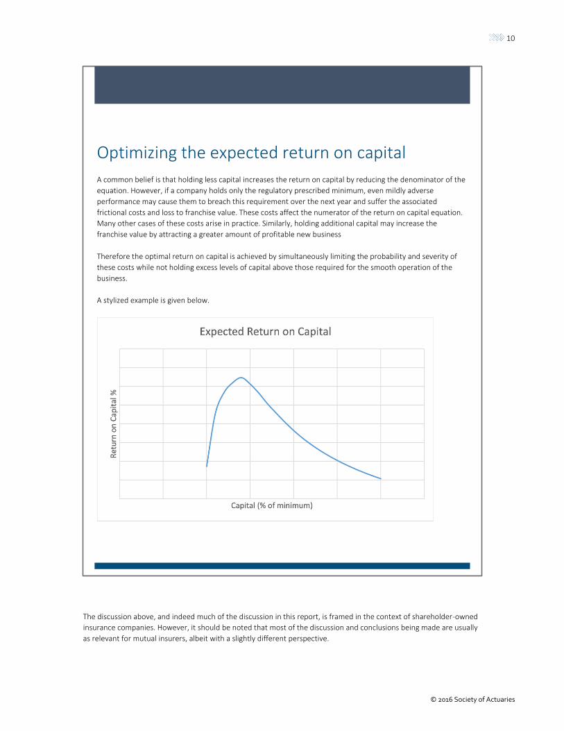
Optimizing the expected return on capital

A common belief is that holding less capital increases the return on capital by reducing the denominator of the

equation. However, if a company holds only the regulatory prescribed minimum, even mildly adverse

performance may cause them to breach this requirement over the next year and suffer the associated

frictional costs and loss to franchise value. These costs affect the numerator of the return on capital equation.

Many other cases of these costs arise in practice. Similarly, holding additional capital may increase the

franchise value by attracting a greater amount of profitable new business

Therefore the optimal return on capital is achieved by simultaneously limiting the probability and severity of

these costs while not holding excess levels of capital above those required for the smooth operation of the

business.

A stylized example is given below.

11


2.3.5 For whom is the EC calculation performed?

Economic capital is the amount of capital required by a company to ensure that certain goals are met with a high

degree of certainty, under a realistic assessment of future risk.

The specific goals, certainty and timeframe depend on the primary stakeholder of interest. This leads to various flavors

of economic capital: Internal economic capital is the type which we will concentrate on for the majority of this report.

This is the assessment of the capital required under the company’s own internal risk assessment, valuation

methodology, objectives, etc. The most important feature of this type of assessment is that the model reflects the

company’s own views business plan and planned management actions. In some publications, the terms “risk capital” or

“internal capital” would be used as an appropriate substitute.

Regulatory economic capital is calculated primarily for a regulator. These bodies’ have the objective of ensuring the

conformity, simplicity and prudence of the model used. They are therefore likely to be more prescriptive in the

application of rules and most interested in the implications to policyholders. Under a prescribed set of economic

assumptions and valuation / projection rules. We classify the Solvency II standard formula and the NAIC Risk Based

Capital regime as broadly falling under this category. We therefore consider a Solvency II internal model to be a mix of

regulatory and internal economic capital assessment since the rules for valuation and risk measurement are strictly

defined and the economic risk assessment, although nominally internal, is heavily guided by regulators.

12


Section 3: EC Methodology and Modeling

3.1 Main Considerations

At its core, economic capital is about projecting a future evolution of the world and the potential impact of adverse

events on business performance, including both the associated costs and the resulting actions taken. The fundamental

question to answer is then how much money would be required today to survive some adversity.

A number of challenges underlie this question, most notably the fact that the underlying variables are difficult to

observe and are altered by actions undertaken over time. This introduces subjective elements into the development of

economic capital models and raises questions about the ability to codify a single global framework, leading many

practitioners to embrace a variety of models that can be built to reflect varying views. Some important areas for

consideration in developing economic capital models are listed and discussed below:

The objectives of the company

The risk drivers that will be used

The risk evolutions that will be considered

Management and policyholder actions assumed

The time horizon for projection

The valuation metrics used

The statistical risk measure

The confidence level

The inclusion of new business

A number of these choices are significant both on their own and in the context of the other choices made. The

following sections discuss each in turn.

3.1.1 Setting objectives

Developing a modelling framework involves asking the questions, “What objectives will define the capital calculation?”

and, “How to reflect these objectives in our capital model?”

These objectives and measures should reflect the real-world behaviors of the company, the mode of possible failure

and the business plan that they follow.

For example, many insurers with long term liabilities follow a buy-and-hold strategy for corporate bond investment

with cash flows used to meet liability payments. Under this strategy the risk to policyholders is that asset cash flows are

insufficient. This includes the impact of possible defaults, rebalancing of the portfolio, re-investment of net proceeds

and potential forced sales to meet policy liability payments or other liquidity requirements. A model that reflects these

risks realistically may choose a cash flow measure as the primary objective and therefore use a long-term, real world

runoff model to measure the primary capital requirement, motivated by the belief that policyholders are better

protected in this way.

Conversely, a company may have a similar set of liability payments but actively hedge market exposures or plan to sell

or hedge risky assets under stress to de-risk and maintain solvency. In this case market risk is of primary importance

and a market-consistent measure is of primary importance. For example the cost of matching risk-free cash flows in 1

year can be calculated, as well as the cost of re-insuring mortality risk etc. In any case some residual risk will remain –

for example, expenses and un-hedgeable policyholder risk. This risk will remain on the insurer’s balance sheet and the

capital available should cover these risks after the cost of de-risking is accounted for.

Other models propose a cost of transfer model. In this case the model tries to estimate the cost of transferring the

assets and liabilities to a willing third party. If this transfer happens then it is usually assumed that the transfer happens

at market- and market-consistent values plus a cost of capital to reflect the third party’s required return on the extra

capital they would need to hold for any remaining risks.

13


3.1.2 Risk drivers

Life insurance companies are subject to a large number of risks. On an individual basis, these risks could include the life

or death of each policy and the performance of each security invested in. As building a model is necessarily a

simplification of reality, the dimensionality of the problem must be reduced to create a representation of reality that is

tractable, understandable and useful in measuring and managing risks. There is some art involved in reducing a highly

complex system to the smallest number of risk factors without excluding features important to the current and future

risk exposures of the entity.

The process involves a combination of grouping and classifying risk families, identifying underlying processes, collapsing

highly correlated risks, grouping exposures into indices, and imposing a structural view of the risk’s dynamics based on

our understanding of its nature. Historical data analysis, expert judgement, academic research and peer benchmarking

all play a part in this process. A balance between model complexity, tractability and usefulness must govern the

selection of risk drivers.

For example, when determining the number of interest rate factors to be used in a 1 year stress model, a modeler will

typically analyze historical data by exploratory methods such as principal components analysis, determining the

number of underlying factors that explain a high percentage of the changes in market yield curves. Typically 2 or 3

factors are found to represent a suitably high percentage of the underlying market risk. They should then consider how

these factors relate to their underlying asset-liability position. For example, the third factor may explain only 2% of the

change in the overall curve but may drive most of the risk in the net value of assets position due to the complex cash

flow profile of assets and liabilities. In this case at least the first 3 factors should be retained as relevant for the EC

calculation. After this analysis, more complex models may be considered that integrate economic structure and logic

into the interest rate model, while retaining the required model complexity.

This simplification of the real world should represent the insurer’s views of how each risk behaves as well as the

underlying dynamics. Then, once these risks are combined into a larger model for measuring the effect that they have

on the solvency of the organization, the model should both mirror expectations and provide new insight into the

complex risk effects, enabling deeper investigations into the dynamics of the enterprise. As each organization is unique

in its business model, product exposure and risk management practices, it is therefore expected that each organization

may have its own unique set of risk factors – retaining the features that are important to the company and simplifying

or eliminating others.

3.1.3 Risk evolutions

After determining the risk factors to include in the EC model, the next step is to develop stresses of these risk factors

and test their effect on the company. This is done through various combinations of stress and scenario testing,

stochastic modelling or historic data analysis.

Stress and scenario testing is common in risk models. These are generally hand-crafted scenarios of the evolution of

risk, formulated by developing a narrative around the scenario – such as a global market crash, natural disasters or

historic periods of market turbulence. These are useful what-if analyses that give insight into the dynamics of the

business and aid our thinking, planning and decision making.

However the use of a small number of scenarios has many limitations. It is very difficult to assign probabilities to these

scenarios and therefore to give an overall confidence for any capital adequacy result derived from them. Further, it is

difficult to check whether the economic scenarios being considered are actually the most important ones for the

business. For example, a smaller equity shock, coupled with a larger interest rate move, may be both more likely and

more severe in relation to profits than a market crash scenario. The ability to test only a small number of scenarios is

especially limiting where exposures are highly geared, with large offsetting asset and liability positions, or in the

presence of complex hedging programs.

Using a stochastic set of scenarios overcomes this challenge. Assigning a joint distribution to the risk factors and then

simulating random outcomes from this distribution produces scenarios that display a wide range of characteristics and

combinations. Passing these scenarios through a model of the enterprise enables an assessment of the risks for the

14


business under many different future evolutions of the world, giving a more accurate view of which scenarios pose the

most risk.

In any method of developing scenarios, there are many human and data biases involved, such as a tendency to ignore

or discount scenarios that deviate from past experience and exclude data from “non-representative” economies. This

manifests clearly in hand-picked scenarios. Because a stochastic model includes more scenarios, more diverse events

and more extreme scenarios in its random outcomes some of these biases and blind-spots can be avoided. However,

another danger lies in the calibration of risk models related to limited imagination and understanding of the world. This

applies equally to deterministic, or stochastic models. Indeed, stochastic models may be seen as more dangerous in

this sense because the assumptions and limitations of the models are more difficult to communicate and require a

greater time commitment to fully understand.

3.1.4 Management and policyholder actions

Management actions may be important to include in the EC model, as they could significantly affect the level of capital

required. They should be as realistic as possible to reflect the actual actions that would be taken by management, both

in benign and extreme market conditions, as it is particularly these actions that will dictate the losses experienced by

the company in the scenarios that drive the required capital.

The management actions assumed in the model should, however be limited to those documented and approved at the

appropriate oversight level. It would be counter-productive, for example to assume in the model that management will

dispose of equity holdings after a market crash if this is not the intention. Such an assumption would lead the company

to underestimate the risk borne and the capital required to support the stated business plan.

Conversely, if risk mitigation strategies are in place which would lead to a reduction in required capital (e.g. dynamic

hedging strategies on VA business), these should not be omitted in the interest of simplicity or prudence. The presence

of these actions will affect the riskiness of each business unit and the diversification of risk between them. Extra

prudence in the measurement of risk or allocation of capital for these products will have the effect of reducing their

risk adjusted return and ultimately lead to sub-optimal decisions. The willingness to commit to management actions is

therefore related to the return on capital. Executing de-risking strategies as conditions deteriorate may involve selling

when markets are down and buying again as they rise, thus resulting in losses. Dynamic hedging is a prime example of

this, but taking out additional reinsurance as a pandemic event unfolds would have similar consequences. Thus, the

presence of management actions in the EC framework can lead to both lower capital and lower returns.

The requirement for only fully approved and documented risk mitigation strategies to be included in the EC model is

often at odds with the need for flexibility and the exercise of context-specific professional judgement – having an

approved rule in place and included within a regulatory EC model could limit the ability of management to exercise

their best discretion when those circumstances appear. In the right environment, this discussion of economic

circumstances and resulting actions can lead to fruitful results – producing a view of EC under a variety of assumptions,

including a minimum set of management actions and an optimal quantitative, efficient-markets view would promote

valuable discussion and should ultimately lead to both enhanced strategic decisions and capital efficiency. In this

process, scenario specific rules chosen to reduce or optimize the level of capital required can be a valuable input to

managements risk contingency planning and improve the speed and quality of reactions to extreme events as they

unfold.

Where extensive reliance on management actions is made, the economic model and assumptions should be realistic

enough to allow the complexity of the management actions to be faithfully modelled, including their possible pitfalls

and limitations.

15


3.1.5 The time horizon

After determining what to project, the next question is how long to project it. Other things being equal, a longer

projection horizon should lead to a more conservative assessment of capital (using the same percentiles, accounting

convention and including intermediate assessments).

Often the time horizon chosen says less about how long the company will remain well capitalized and more about the

valuation metrics used, management actions assumed and business planning horizon.

One approach is to project forward for the lifetime of all business on the books. This is theoretically appealing, as it

matches the long term nature of typical life insurance policies. The risk profile of certain types of business may change

significantly in the future too. For example as rider benefits are taken up or returns locked in, an existing block of

business may naturally become riskier without any change to risk management policy or practice. Using a longer time

horizon can help ensure that the capital held is appropriate to cover the business through this evolution.

In reality, however, the choice of a time horizon is usually driven by the type of accounting measures used, the

business planning horizon and the risk mitigation strategies undertaken or planned. Some considerations for choosing

the time horizon are:

Where only cash flows are used without intermediate or terminal valuation, is a full runoff of the business

required?

Alignment of the business planning period and the EC projection period allows the projection to have a basis in

more formalized business plans, which helps management with the alignment of risk appetite to the levels of

economic capital required. This alignment would be difficult over a longer time horizon.

Considerations of the time horizon over which risk mitigation actions would or could be taken should influence the

choice of time horizon. For example, if all risks are fully hedgeable in capital markets in a short time horizon and a

market consistent liability measure is used, then a short projection period maybe sufficient to describe the risks

faced. In contrast, if a valuation measure is used that does not recognize losses for a number of years (like some

book value accounting systems), then a longer projection period which allows the full evolution of risks to unfold

may be needed.

3.1.6 Valuation metric for intermediate valuations

Where EC models use a valuation metric for assessment of intermediate value of assets required, there are a number

of alternatives that are possible. For example, a market consistent measure may be used to value assets and liabilities

consistently with the market prices of assets and derivatives. Many insurers use a “market based” measure of value in

addition to or instead of this stricter market consistent measure. This type of valuation typically attempts to account

for the company’s own view of the economic value of the value of assets and liabilities by making adjustments to

market discount rates, implied volatilities etc. to reflect the unique features and business plans of the company. For

example, where the assets backing a particular liability portfolio are very actively traded or hedged in the market, it is

usual to use pure market consistent techniques to value both. However where liabilities are long term and the assets

are considered to be hold-to-maturity, it is common to adjust either asset or liability valuations to diverge from strict

market-consistent pricing.

Other valuation measures may be used. For example accounting measures which take assets at book value and try to

discount liabilities on a consistent basis are also sometimes used as intermediate measures in practice. The precise

valuation metric used should be linked to the objectives of the economic capital model. Rather than being dogmatic

about the exact definition of value or capital, we believe that the size of, and change in the capital measures over time,

are often the most useful outputs from an EC model.

Other intermediate metrics that may be measured in the economic capital projection include statutory reporting

requirements like regulatory capital or insurance reserves. More complex capital models may integrate multiple

16


objectives into the calculation. Section 6.3 introduces this idea in the context of multiple valuation measures within a

risk appetite framework.

3.1.7 The statistical risk measure

The choice of statistical risk measure is an important choice for the model design. While a line-up of statistical risk

measures are available, the two most common in use are value-at-risk (VaR) and conditional tail expectation (CTE). CTE

is also known as tail value-at-risk (TVaR).

The VaR measure is a straightforward percentile of the loss that an insurance company may experience. It prescribed in

the Solvency II standard formula and almost universally adopted in companies using internal models. Alternative

approaches are permitted within internal models but only if offering greater security than the VaR metric. While VaR

has a number of advantages (see end of this section), it does have some shortfalls. Technically speaking, it is not a

coherent2 risk measure – which is to say that it does not satisfy a number of desirable properties of risk measures. Most

important among these is that it does not consider the size of losses in excess of the measured percentile. This means

that a company may be exposed to low probability events that would cause losses only slightly more than their

available assets or at a scale that could devastate a national or global financial system - without any difference in their

capital requirement. This feature is a clear incentive to take on low probability, high severity risks which give a higher

return on capital profile in a VaR based EC model. These are in many ways the most dangerous risks because of the

difficulty in estimating their probability of occurrence.

More mathematically, the VaR measure in general lacks the property of sub-additivity, meaning that in some cases this

measure can fail to reward diversification of risks, particularly in the presence of events with low probability and high

severity3. This is problematic both in theory and in practice, limiting the ability to allocate risk to the business units,

products and sources from which it arises.

These limitations are solved by using a CTE metric, measured as the probability weighted average of possible losses in

excess of a given percentile. This corrects the failure of VaR to consider and allocate capital to extreme risks. It also

allows better recognition and allocation of diversification benefits.

This improvement in theoretical coherence comes at a cost for practical implementation. There is greater difficulty in

explaining the measure to a non-technical audience, or sometimes even to a technical audience. In addition, a CTE is

more difficult to handle numerically – for accurate assessment it is required to measure the whole tail of the risk

distribution and the effect on the company in all extreme circumstances. Any model limitations or quick

approximations which could be acceptable in a VaR model could end up unintentionally driving the capital result under

a CTE measure.

3.1.8 The confidence level

The aim of insurance regulation and capital is not to have a zero failure system, as the only way to ensure this would be

to avoid all risk entirely. Instead, the objective is to reduce the likelihood of failures up to the point where the marginal

cost of additional failure prevention exceeds the additional benefit of safety. Some compromises may be necessary in

this decision, as different stakeholders may have different tolerances for failure.

Risk appetite statements and fundamental corporate philosophies should ultimately drive the decision of selecting a

confidence level by contemplating the vision for what the company aims to achieve and the implications of succeeding

or failing in this mission. Translating this from an abstract exercise into a tangible decision requires an understanding of

2 Artzner, “Coherent Measures of Risk” https://people.math.ethz.ch/~delbaen/ftp/preprints/CoherentMF.pdf

17


the likelihood and severity of risks; therefore, EC models play an important, and often iterative, role in informing this

decision.

Where a multi-year measure is used, the confidence used should (other things being equal) reasonably be lower

because it relates to a probability of ruin over a longer horizon. To put it another way, providing the same level of

protection against company failure over a longer horizon requires more resources than providing against company

failure over a shorter horizon. This further highlights the important relationship between modeling assumptions and

modeling implementation.

3.1.9 New business

Including new business in the projection may be important, especially for longer term models and companies writing

significant volumes. The reason relates to the tendency of management to write new business up to their comfortable

capitalization levels. For example, in good times the business may generate a high level of surplus capital. It would then

be natural to write new business or make extra distributions to policyholders or shareholders to enhance the return on

capital. If these features are not included in the long term projection these scenarios would tend to never see ruin,

whereas if a more realistic path were incorporated, they would be as likely as other scenarios to ruin because risk

would be increased to the point where they were as risky as average paths. This feature may have the effect of

significantly understating risk in a runoff model. Over time, however, new business should also increase available

capital in scenarios where it is written profitably. Achieving a sufficiently realistic representation within a runoff EC

model is needed.

A 1 year or intermediate term model aligned with the business planning horizon is more tractable in this context

because it can point to an explicit business plan and agreed actions for the management of the business. There is less

uncertainty about future management plans, insurance regulations, market regimes etc.

3.1.10 Putting it all together

Once all the above factors are considered, constructing an economic capital model is a task of representing the views

and needs of the company in a coherent, realistic and parsimonious way.

In practice, two broad methodologies have emerged as the most common: a liability runoff approach and a finite risk

horizon approach. Most insurers calculating EC today do so following one (or sometimes both) of these approaches.

While specific definitions and calculation approaches can vary widely, the two approaches can broadly be defined as

follows:

The liability runoff approach, where EC represents the current market value of assets required to pay all future

policyholder benefits, and associated expenses, at the chosen security level (expressed on a VaR or CTE basis), less

the current value of the liabilities (typically defined on a mean or best estimate basis).

The finite risk horizon approach, where EC represents the current market value of assets required to ensure that

the value of liabilities (typically market consistent), can be covered at a finite point in the future (typically one

year), at the chosen security level, less the current value of the liabilities.

3.2 The Liability Runoff Approach

While there are a number of approaches to implementation, the liability runoff approach is typically performed using a

stochastic simulation method as follows:

A set of (typically 1,000 or more) future scenarios for the runoff of the business is defined. The scenarios include

specifications for economic and demographic conditions, including risk drivers such as interest rate scenarios and

18


asset default rates. Mortality levels and other insurance risk drivers may also be included in the stochastic

scenario generation process.

The scenario distribution is a realistic assessment of the future risks and returns expected on each asset class or

risk driver.

Projected asset and liability cash flows are developed for each scenario, including realistic management actions,

product rules and policyholder behavior.

Intermediate valuations or required reserves for each time period and scenario are calculated (as required by the

capital definition)

Under each scenario, the level of assets required at the beginning of the scenario to satisfy all obligations through

to the end of the projection is determined.

These obligations may include paying policyholder cash flows, debt payments and dividends; having sufficient

funds available to meet regulatory reserve or capital requirements; having sufficient funds available to maintain a

minimum credit rating or other management objectives.

Assessing many of these intermediate objectives implies a nested stochastic calculation within the EC model. For

example, assessing a reserve which is calculated as a runoff CTE within the runoff EC model may require 1,000

scenarios repeated at each projection year.

The level of required assets includes consideration of the investment returns earned on those assets (including

investment strategy and re-investment considerations). This is equivalent to discounting future excess obligations

at the return earned on the excess capital assets.

The level of “required assets” for all scenarios is then ranked to form a distribution.

EC is defined by applying the chosen risk metric (e.g., VaR or CTE) to this distribution of total required asset levels

and deducting the current value of the liabilities, measured on the selected basis (typically mean or best

estimate).

Insurers using a runoff approach are increasingly pursuing the development of fully integrated stochastic models, in

which demographic and economic assumptions vary stochastically within the same model. This has distinct advantages

for capturing risk interactions within the EC model. For example, scenarios with high longevity and low interest or

investment returns will lead to a capital requirement in excess of the sum of the requirements should either of these

events occur in the scenario individually. This interaction drives the capital result. This level of integration makes use of

relatively new models of the stochastic evolution of insurance risks such as stochastic mortality and morbidity models

or predictive models for policyholder behavior4. These stochastic models of insurance risk are a significant

improvement on older approaches for including insurance risk in runoff models. Under these approaches, a stress

would generally be conducted for mortality rates (for example) at time 0 and the effect on insurers’ liability value

determined. This static, T0 stress would then need to be combined with the runoff risk calculation in a necessarily

approximate way.

The liability valuation basis used to define EC under the runoff approach can vary, with a different valuation basis

resulting in a different split between liabilities and EC (but the same level of total “required assets”). In practice, mean

or best estimate liability valuation bases are popular choices of liability valuation basis. Note that the most important

measure for the purpose of policyholder protection is the required assets; the split of required assets between

liabilities and EC is unimportant from this perspective, although will be relevant if EC is to be used in other contexts.

A few different variations of the liability runoff approach are observed in practice, in particular the inclusion of

requirements to meet interim solvency measures during the runoff. In its basic form, the liability runoff approach

considers the asset level currently required to pay all claims and expenses throughout the runoff period, and does not

explicitly take into account solvency levels at interim dates. Without any checks of interim solvency, there is an implicit

assumption that adverse experience in earlier time periods can be offset against positive experience in later time

periods. Put another way, the methodology allows the insurer to become technically insolvent in interim years

providing it rebounds before the end of the runoff. This ignores the potential impact of regulatory intervention or

reputational damage at times of technical insolvency.

4 Cainrs, Blake, Dowd Modelling and Management of Mortality Risk: A Review

19


Alternatively, the liability runoff approach can incorporate a check on solvency at interim points during the runoff. This

raises the additional questions as to what measure of interim solvency should be used and how frequently it should be

assessed. If the economic principles underlying the methodology are to be maintained, an economic basis of interim

solvency would be required, which can be computationally intensive.

3.3 The Finite Risk Horizon Approach

The finite risk horizon approach is typically performed as follows:

An economic balance sheet is developed as of the valuation date. The difference between the value of assets and

value of liabilities gives the economic value of net assets, i.e., the available capital at the valuation date measured

on an economic basis.

For a number of real world scenarios, assets and liabilities are projected forward over the length of the risk

horizon (e.g., one year), at which point a projected economic balance sheet is developed. The resulting projected

economic value of net assets (positive or negative) is then discounted to the valuation date using the projected

earned investment return over the year in that scenario.

A negative discounted value quantifies the additional initial asset value the insurer needs to hold to ensure it

remains solvent on an economic basis at the end of the year under that scenario. A positive discounted value

quantifies the excess initial asset value over the amount needed to ensure solvency on an economic basis at the

end of the year. The discounted value (of the projected economic value of net assets) is therefore subtracted from

the value of assets at the valuation date to give the required assets for that scenario.

As with the runoff approach, the finite risk horizon approach can be implemented using stochastic simulation. The

steps described above are performed for a large number of real world scenariosperhaps 100,000 or more given the

higher security levels that would typically be used under shorter risk horizons. This gives a distribution of required

assets by scenario, from which the overall level of required assets can be determined (i.e., by calculating the chosen

risk measure at the target confidence level). The EC requirement is then determined by deducting the initial value of

the liabilities from the required assets.

It is also common to implement the finite risk horizon approach using stress tests as an approximation to stochastic

simulation. This has tended to be more common for business with significant financial options and guarantees where

the market-consistent value of liabilities requires the use of a risk neutral stochastic valuation. To implement a

stochastic risk horizon approach to EC would therefore lead to computationally challenging “stochastic on stochastic”

calculations (although proxy modeling techniques have now been developed to overcome this, as discussed in Section

7).

With a stress testing approach to implementation, the full, accurate multi-dimensional distribution of required capital

described is not developed. Rather a limited number of stress scenarios are run, where the scenarios have each been

calibrated to the chosen security level. Scenarios are chosen to explore each of the key risks, and the capital results for

each risk are typically combined using a correlation matrix.

It is important to note that even under the finite risk horizon approach, a runoff projection is still required, since a

terminal value of liabilities at the end of the risk horizon is needed. Future uncertainty surrounding the risk beyond the

risk horizon is captured within the value of the liabilities at the end of the year. This may consist of both the time value

of options and guarantees as well as the cost of capital required to support that uncertainty.

While the finite risk horizon approach originated with the banking industry’s use of short term market consistent

calculations, it has also been adopted by many European multinational insurers and their global subsidiaries, which

include many significant North American insurers. It is now being adopted as the basis for insurer solvency regulation

across Europe under Solvency II. A number of large North American insurers are also adopting this approach to EC

calculations.

20


Due to the common use of a mark-to-market balance sheet, the finite risk horizon approach can be sensitive to market

conditions and prices. Some consider that this results in market movements, particularly those driven by changes in

market sentiment, having undue influence in setting capital requirements, given the long-term nature of a life

insurance business. Others see the link to market prices as an advantage, both because they reveal the true market

volatility of the balance sheet and because these prices may be very relevant when assessing risk management options

available in adverse scenarios.

3.3.1 Market consistent approach for terminal valuation

Market consistent or similar valuation methodologies have become the most common method of allowing for terminal

balance sheet valuation globally. This adoption has been largely driven by European regulators who have mandated its

use in Solvency II capital calculations (although adjustments are allowed that make the result closer to market-based

than market consistent).

The use of a terminal valuation methodology in an EC perspective implies it can be used as the basis for securing the

payment of benefits to policyholders or capturing a view of the liability. Any measure that does not realistically relate

to these objectives is of little practical use. This does not prevent the use of multiple valuation metrics for different

other purposes in the model, for example, statutory reserves may serve as intermediate tests within a projection that

could trigger certain regulatory or management actions or require balance sheet strengthening. However, the ultimate

valuation metric that drives the capital requirement must relate to the ability to pay claims.

A market-consistent measure has many theoretical virtues and addresses many of the issues with a runoff approach,

but some substantial questions and issues remain. For background, a brief summary of market consistent valuation

practices is included below for the purpose of highlighting elements important to the EC calculation.5

In a market consistent valuation, the insurer aims to value liabilities in a way that is consistent with market prices. This

means that:

Future cash flows that are certain or guaranteed are discounted at market risk-free interest rates. While there is

some debate between whether treasury or swap rates should form the basis of this risk free discount rate, this

debate is beyond the scope of this paper.

Where liabilities have contingent cash flows such as embedded options or variable guarantee features, their value

is included in the liability valuation in a way that is consistent with the market prices of similar options or using

similar valuation methods.

Assets are accounted for at market observed prices (or using a mark-to-model basis where prices are not readily

observable).

There is an allowance for the cost of capital, for non-hedgeable risks, that a willing buyer would need to hold to

take on the liabilities.

In theory this valuation basis gives a valuation of an insurer that is consistent with market prices and therefore gives a

value close to that which a willing buyer and seller in the market would transfer the assets and liabilities of the

company in an arms-length transaction. This should also give a valuation for assets and liabilities which can be “locked-

in” through risk transfer or capital markets transactions. For example, bonds or swaps should be able to be purchased

to exactly match guaranteed cash flows; derivatives traded that exactly pay for options offered to policyholders;

reinsurance purchased that removes the risk of adverse mortality and morbidity experience etc. Some risks however

remain, such as policyholder behavior, for which there are a very limited set of willing buyers.

The benefit of this argument for EC purposes is that, when considering risk to the market consistent balance sheet over

some time period (e.g. 1 year), the insurer should be able to completely de-risk the balance sheet at that point. This

means there would be no need to consider future economic risk (because there would be none, and any risk would be

5 Wilson, Value and Capital Management: A Handbook for the Finance and Risk Functions of Financial Institutions

21


assumed voluntarily or at the discretion of the regulator who would be in control at that point). This also means that

the terminal value measure is aligned with actions that can or would be taken in the market to mitigate risk and protect

the company in adverse circumstances.

There are, however, issues with this approach. When looking at market based rates and prices, it is usual to analyze

frequently traded assets and liquid derivatives. While these are more standardized, traded and compared, they are

fundamentally different from insurance liabilities. This has led to concern from many insurance companies who argue

that this valuation measure does not take account of the economics of long term insurance contracts. In particular, the

insurance company has use of the policyholder funds for long periods of time with no obligation to return it without

penalty (or very low likelihood of significant outflows due to policyholder behavior). Over this time the shareholders

benefit from the investment returns earned on the backing assets. This long term funding and the option to change

investment strategy have value to the company. However, a formal, consistent and broadly agreed framework for its

measurement has not been developed – some argue for an addition of a liquidity premium to reflect asset or liability

illiquidity; others for a recognition of the excess returns that are expected to be earned by holding the assets over the

long term. Whatever the underlying theory, the mechanism of the adjustment is typically represented by an addition to

the risk free rate for discounting liability cash flows.

Conversely, holding life insurance liabilities attracts a regulatory (and economic) capital requirement. The cost of

holding this capital against risks that cannot be perfectly hedged is often included in valuations (both base and

stressed) for economic capital purposes. In this way, both the benefit and cost of the specific business environment can

be reflected in the valuation measure.

In addition to identifying the rate at which cash flows should be discounted, there are issues related to the

completeness of markets for benchmarking liabilities. For example, life insurers typically have liabilities that go out for

many years longer than the assets available for benchmarking. Even where swap rates are quoted for the full term of

the liabilities, there are questions by many of the validity of these quoted rates or the willingness of banks to transact

at these prices in sizeable volumes. Some models address this through the liquidity premium or comparable

adjustments to risk-free rates.

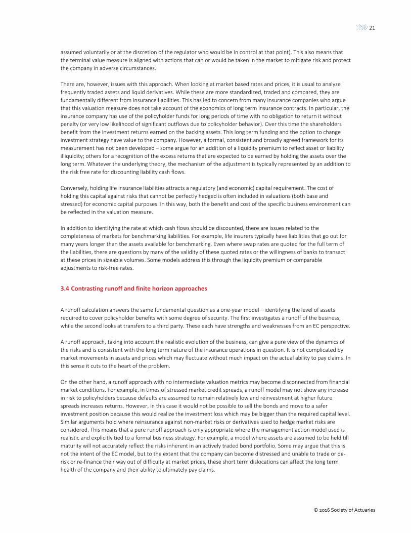
3.4 Contrasting runoff and finite horizon approaches

A runoff calculation answers the same fundamental question as a one-year model—identifying the level of assets

required to cover policyholder benefits with some degree of security. The first investigates a runoff of the business,

while the second looks at transfers to a third party. These each have strengths and weaknesses from an EC perspective.

A runoff approach, taking into account the realistic evolution of the business, can give a pure view of the dynamics of

the risks and is consistent with the long term nature of the insurance operations in question. It is not complicated by

market movements in assets and prices which may fluctuate without much impact on the actual ability to pay claims. In

this sense it cuts to the heart of the problem.

On the other hand, a runoff approach with no intermediate valuation metrics may become disconnected from financial

market conditions. For example, in times of stressed market credit spreads, a runoff model may not show any increase

in risk to policyholders because defaults are assumed to remain relatively low and reinvestment at higher future

spreads increases returns. However, in this case it would not be possible to sell the bonds and move to a safer

investment position because this would realize the investment loss which may be bigger than the required capital level.

Similar arguments hold where reinsurance against non-market risks or derivatives used to hedge market risks are

considered. This means that a pure runoff approach is only appropriate where the management action model used is

realistic and explicitly tied to a formal business strategy. For example, a model where assets are assumed to be held till

maturity will not accurately reflect the risks inherent in an actively traded bond portfolio. Some may argue that this is

not the intent of the EC model, but to the extent that the company can become distressed and unable to trade or de-

risk or re-finance their way out of difficulty at market prices, these short term dislocations can affect the long term

health of the company and their ability to ultimately pay claims.

22


A one-year model, at least when implemented using market consistent valuations, is inherently more aligned with

financial markets and therefore with market-based risk mitigation strategies that can be or are being undertaken. This

may include financial derivatives, reinsurance or securitization transactions. This alignment is also beneficial from a

transparency and comparability point of view. The disadvantage being that this strict adherence to market principles

may come at the cost of consistency with long term insurance-specific features or the actual business model of the

insurer.

To bridge the gap between one year and run-off views, adjustments have been made in both directions. Market-based

valuation approaches (particularly in Solvency II) have employed an addition to the risk-free discount rate that varies

with the economic environment. For example, when credit spreads are high, the spread adjustment increases. These

adjustments are applicable only for certain classes of business.

This spread adjustment attempts to correct the market-consistent regime in a way that is cognizant of the particular

type of insurance portfolio under consideration. The effect is to assume that the insurer is only exposed to changes in

default or downgrade expectations (measured cumulatively over the life of the portfolio) on credit-risky bonds and that

changes in bond prices or spreads from other sources (like changes in actual or perceived liquidity; changes in risk

premium demanded by investors; changes in markets’ default expectations etc.) are offset by the adjustment made on

the liability discounting side. The end results is a set of assumptions (and an effect) very similar to the starting point of

a runoff cash flow model – that the company is exposed to the risk of cumulative defaults but that changes in the

market prices of assets or spreads are not important for the company’s ability to pay claims.

Under either regime, the company’s expectation of future (average and worst case) defaults can be dependent on

market observed values – to the extent that the company believes that market prices reliably embed expectations of

future performance. Viewed another way, both the adjusted market-based and runoff cash flow methodologies embed

strong assumptions about the mean reversion of asset returns after extreme market events.

This mean reversion theme is present in other senses too. A runoff model will typically make an assumption about the

expected level of yield curves based on historic experience that is different from the future level implied by the long

end of the initial market yield curve. Whereas the Solvency II adjusted market-based model incorporates these effects

by ignoring parts of the initial yield curve and extrapolating quickly to real world expectations. The effects of both are

to introduce a type of mean reversion into the measurement of capital that diverge strict short term market pricing or

market implied risk levels.

The nature of this mean reversion assumption is highly subjective and difficult to reliably estimate. The evidence for

these effects is also mixed and dependent on the particular time periods, asset types and economies included.

Other than these important effects, the models behave in different ways. A runoff model looks at the tail of the

outcomes over time whereas a one-year model looks at the average after a big stress and change in expectations.

These approaches naturally vary in the levels of capital they output and in the sensitivity of the capital result to changes

in economic conditions. From a consistency sense, where companies have a strong view about long term investment

and mean reversion of returns, the runoff model is a more natural model choice, allowing the user to directly input

their assumptions and observe the result based on the full dynamics of the projection, whereas the market based

adjustments are more difficult to estimate and often derived by equating to the result of a runoff projection with

limiting assumptions about future actions.

An additional consideration is the degree to which the capital estimates produced by these two types of models vary

with changes in market conditions and therefore promote or defend against cyclicality in global capital markets. Pure

market consistent one-year regimes may promote more cyclical investment markets if companies exposed to these

regimes and therefore larger swings in capital ratios are encouraged to sell risky assets more quickly in times of

distress. When one-year or runoff cash flow regimes are compared, the degree of cyclicality varies and is inherently

controlled by the degree of mean reversion or equivalent market adjustments assumed.

3.5 Risk Aggregation

23


3.5.1 Overview

Risk aggregation refers to the process by which risk exposures or capital requirements at lower levels (e.g., individual

risks, business units, or geographic regions) are consolidated to higher levels (e.g., the enterprise total or various

subtotals). Typically the required EC result for the total enterprise is less than the sum of the individual risk exposures

due to diversification benefits, which arise from imperfect correlation between risks—loosely speaking, the likelihood

of two extreme events occurring simultaneously is generally lower than the likelihood of each one occurring

individually. A special case of this is offsetting risks, when risks are negatively correlated. For example, an insurer who

writes both life insurance (negatively impacted by an increase in mortality) and payout annuities (positively impacted

by an increase in mortality) to similar classes of individuals will generally experience a reduction in overall mortality risk

exposure.

Diversification across distinct business portfolios is influenced by the relative shapes of the loss functions with respect

to risks. If loss functions are nonlinear—meaning the impact of a stress scenario grows at an increasing rate as the size

of the stress increases—then diversification ratios are generally lower under more extreme risk metrics because the

increasing contribution of the nonlinear variable has a greater influence on the total capital result. This impact on

aggregation generally becomes more pronounced as the loss function becomes steeper.

Although a range of aggregation techniques are used in practice, they can broadly be classified into two approaches.

3.5.2 The Flat Correlation Matrix Approach

Under the correlation matrix approach, standalone capital is calculated for individual risk factors—often by

deterministic stress testing at a targeted confidence level—and then aggregated by multiplying the capital results

through a correlation matrix using a formula similar to the following:

𝐸𝐶𝑡𝑜𝑡𝑎𝑙 = √𝐸𝐶𝑅𝑖𝑠𝑘1

2 + 𝐸𝐶𝑅𝑖𝑠𝑘22 + 2 × 𝐶𝑜𝑟𝑟(𝑅𝑖𝑠𝑘1, 𝑅𝑖𝑠𝑘2) (3.1)

This can be generalized to multiple risks using standard matrix algebra:

𝐸𝐶𝑡𝑜𝑡𝑎𝑙 = √𝐶𝑇(𝑀𝐶) (3.2)

Where C is a column vector of standalone capital amounts by risk, and M is a correlation matrix for those risks. Due to

the formulas involved, this approach is also referred to as “sum of squares aggregation” or the “variance-covariance

approach.”

The advantage of the correlation matrix approach is its ease of calculation; however, it has some limitations.

Correlation assumptions are often set by some combination of historical data or expert forecasts that analyze the

relationship between risk scenarios; however, these correlations are applied not to the scenarios themselves, but

instead to the standalone capital amounts. The implication of this approach is that balance sheets respond linearly to

risk scenarios, which can be a severe approximation for some types of business, creating a diversification amount which

is a function of individual exposures rather than the underlying relationship between risk drivers.

Another limitation is that consistency of correlations is not enforced. All correlation matrices, regardless of the

application, must be positive semi-definite (PSD), which is a mathematical property to ensure that correlations are

internally consistent—otherwise, it could contain impossible relationships where two highly correlated risks are

24


oppositely correlated with a third risk. Although non-PSD correlation matrices are meaningless in reality, the

aggregation formula will continue to “work” in the sense that the calculation can be performed and a total EC result

produced. The burden to separately check the matrix falls entirely on the user of the formula, which is both easy to do

and easy to overlook.

An extension of the correlation matrix approach is the “tiered correlation matrix approach” or “stepwise aggregation.”

Under this approach, individual risk factors are grouped into categories (e.g., market risk and insurance risk).

Aggregation is first performed within each category, then across risk categories, with both steps using Equation 3.2 The

advantage of a tiered approach is that fewer correlation assumptions are required:

Exhibit 3.1: Correlation Assumption Structure

The disadvantage of a tiered approach is the calibration of correlation assumptions between risk categories. Although

data may be limited, the theoretical concept of a correlation between any two individual risks is straightforward; in

contrast, it is difficult to explain the mathematical interpretation of a correlation between two (or more) matrices, and

consequently it can be challenging to create and validate the higher level assumptions.

Some companies also use this type of approach to measure aggregation and diversification between geographic

regions or lines of business by declaring correlations between these elements of the corporate structure. From a

calibration perspective, this shares a similar disadvantage with the tiered correlation structure in that it is unclear

mathematically what is actually being measured in a correlation between two portfolios, which themselves are not

random variables but rather are a set containing different random variables. Nonetheless, once these correlations are

defined, the matrix multiplication calculation is straightforward to perform as an approximation, though reconciliation

with risk diversification calculations can be an additional challenge.

3.5.3 The Scenario Aggregation Approach

The scenario aggregation approach involves the use of integrated scenarios containing multiple risk factors. Because

the resulting financial impact from any given scenario reflects an aggregate result across the risks, EC calculated from

the distribution of scenario results implicitly reflects diversification benefits. Note that scenario aggregation does not

eliminate the need for correlation assumptions; rather, it pushes that assumption out of the aggregation function and

into the scenario file creation process.

The dependency structure underlying the projection scenarios may be more complex than a simple correlation matrix,

and the use of copulas is growing. While a detailed discussion of copulas is outside the scope of this report, in an EC

context they effectively serve as dynamic correlation matrices, with the ability to increase (or decrease) the strength of

the dependency associated with tail events. For example, the belief that markets crash together during periods of

Market

Risks Ris

k 1

Ris

k 2

Ris

k 3

Ris

k 4

Ris

k 5

Risk 1 1.00 # # # #

Risk 2 # 1.00 # # #

Risk 3 # # 1.00 # #

Risk 4 # # # 1.00 #

Risk 5 # # # # 1.00

Insurance

Risks Ris

k 6

Ris

k 7

Ris

k 8

Ris

k 9

Risk 6 1.00 # # #

Risk 7 # 1.00 # #

Risk 8 # # 1.00 #

Risk 9 # # # 1.00

Risk

Categories Mark

et

Insura

nce

Market 1.00 #

Insurance # 1.00

All Risks Ris

k 1

Ris

k 2

Ris

k 3

Ris

k 4

Ris

k 5

Ris

k 6

Ris

k 7

Ris

k 8

Ris

k 9

Risk 1 1.00 # # # # # # # #

Risk 2 # 1.00 # # # # # # #

Risk 3 # # 1.00 # # # # # #

Risk 4 # # # 1.00 # # # # #

Risk 5 # # # # 1.00 # # # #

Risk 6 # # # # # 1.00 # # #

Risk 7 # # # # # # 1.00 # #

Risk 8 # # # # # # # 1.00 #

Risk 9 # # # # # # # # 1.00

All-risk correlation assumptions Tiered correlation assumptions

25


financial stress can be reflected by an individuated T-copula, which contains a standard correlation matrix-style

dependency assumption plus additional parameters to increase tail dependence.

3.5.4 Measurement of the Diversification Benefit

While most EC calculations will give an overall capital requirement, it is useful and informative to additionally measure

the amount of diversification benefit achieved by the company through exposure to imperfectly correlated risks. A

benefit to companies with many sources of risk is that their capital requirement will be lower, on aggregate than

companies with highly concentrated risk. This recognizes the phenomenon that it is unlikely that an insurer will lose

money on all risk simultaneously. So to the extent that the risks are uncorrelated or negatively correlated, capital held

against one risk is able to offset losses from other risks. This diversification effect makes companies with many lines of

business and well diversified portfolios more capital efficient than companies with lesser diversification.

The standard method to assess the level of diversification benefit is to analyze each individual risk on a stand-alone

basis. The total un-diversified capital requirement is the sum of these risks, representing the amount which would be

held if all risks were perfectly correlated. The diversification benefit is the total capital minus the actual EC

requirement. This calculation is generally straightforward to perform and analyze but masks a large degree of model

definition and risk driver assumptions in its execution.

The level at which risk drivers are defined makes a difference to the calculated diversification benefit. Although, when

done correctly, the level of granularity does not significantly influence aggregate results, the diversification benefit will

be reported as the difference between those aggregate results and the lowest level of granularity available, thereby

being influenced by the model structure. For example, if 100 different equity assets are modeled explicitly, there will

be some measurable diversification between them; in contrast, if an equity portfolio were modeled as a single unit,

inherent diversification between the individual assets would correctly be captured at the portfolio level, but

information would not be available to explicitly report those diversification benefits. For this reason, diversification

benefits and diversification ratios may be useful as internal metrics, but they are less meaningful for external reporting.

This conclusion is even more pronounced when looking across different insurer types or industries.

3.6 Pros and Cons of EC Approaches

3.6.1 Risk Management

The risk that policyholders do not receive their contractual entitlements in full is a function not only of the level of

capital held by the organization but also of the way the organization is managed. Turning this around, the EC required

by an organization can be seen to be a function of the actions it will take in managing risk as well as the selected level

of security. This interaction between the calculated EC measure and the strategies adopted for managing risk within

the organization is an important aspect and one in which the two primary approaches to EC take very different

approaches.

The finite risk horizon approach examines a short period (e.g., one year) during which adverse experience emerges and

during which there is an explicit assumption that limited management actions are taken. Such actions would typically

be limited to a degree of trading of assets, to the extent that the organization has specific programs or strategies in

place to perform such trades as markets develop (e.g., dynamic hedging strategies). At the end of the one-year period

there is an assumption that the risk can be “closed out” by market transactions, through risk reduction (e.g., hedging of

market risks), risk transfer (e.g., reinsurance) or through a sale of the portfolio to a third party. This ability to close out

the risks at the end of the year is what commonly drives the use of a market consistent balance sheet.

Risk emergence over a longer time horizon is not examined directly by the finite risk horizon approach (although the

valuation of the liabilities does bring in information about these risks and how they might be managed). Similarly, the

multitude of other management actions which are available over the longer term are excluded from the calculation,

26


including variation in the asset strategy, the reinsurance strategy, the volume and pricing of new business, and the

ability to raise additional capital or restrict shareholder dividend payments.

This is not to say that organizations adopting a finite risk horizon approach do not recognize the need to address

longer-term risk issues and their potential consequences in terms of capital. They typically prefer to address such issues

through a scenario analysis of projected EC assessments over a business planning cycle (e.g., three to five years),

bringing in all the range of management actions that might reasonably be taken in each scenario. So, for example, a

prolonged period of poor equity returns might be considered, revealing a deteriorating capital and security position if

no action were to be taken. However, the management actions described above may be available in such a scenario,

and it would appear reasonable for management to rely on their utilization, instead of holding additional capital at the

outset to cover such a risk.

The stochastic liability runoff approach on the other hand does bring in all risks during the runoff of the portfolio, albeit

often only those relating to the existing portfolio (sometimes with a limited number of years’ new business also

included). A number of the actions available to management during that period may also be allowed for through

formulae included in the stochastic model. However, it is very rare for the full range of such actions to be incorporated,

as it is difficult to allow formulaically for such actions as additional capital raising and increased utilization of

hedging/reinsurance, as the capital position of the organization varies over time; also for the ability to vary new

business volume and prices in circumstances where new business is modeled.

In this context a number of pros and cons can be observed.

The finite risk horizon approach gives strong recognition to the fact that an organization’s principal ability to

control risk in the short term is through trading assets and/or liabilities, including through reinsurance and

portfolio/business transfer. However, the lack of data available to calibrate a distribution of market-consistent

prices for non-hedgeable liabilities such as mortality/morbidity may be regarded as a potentially significant

weakness.

The liability runoff approach, on the other hand, can give insufficient recognition to this ability to control risk

through asset/liability trading, unless sophisticated algorithms are built into the model to allow for it.

The finite risk horizon approach relies on deterministic adverse scenario analysis to examine longer term risks and

their management. This has a weakness in that it is reliant for its completeness on management’s scenario

selection (as opposed to using a stochastic scenario generation process), but has a strong advantage in allowing

management to make a realistic assessment and communication of all the risk management actions it might take

in such a scenario. Management can then make a conscious choice between taking such action and holding

additional capital, additional to initial EC assessment, effectively to cover their preference not to take such

management action.

The liability runoff approach aims to build longer-term management actions into the stochastic model, although in

practice this can be difficult to perform comprehensively. While this approach removes the reliance on

management scenario selection, stochastic projections of longer-term risk emergence and management thereof

can be less clear and more difficult to analyze than with a deterministic equivalent. There is a risk that EC can be

overstated through the omission of actions that might reasonably be taken, or alternatively that the reason for the

high capital requirement (a preference for, or an assumption of, less risk management action) is not clearly

understood. In addition, in an environment where management changes can occur fairly frequently, making

assumptions as to management actions over the longer term can be considered speculative.

Regardless of risk management actions that may be taken in the future, the reality of capital management and

regulatory reporting is that required capital will be calculated on (at least) an annual basis. When applied over a

one-year time period, the finite risk horizon approach acknowledges this reality and better aligns itself with the

actual management of the company. In contrast, the liability runoff approach attempts to find the amount of

capital today that will provide sufficient protection for the lifetime of the portfolio, thus ignoring the reality that

capital levels will be annually reevaluated.

A finite risk horizon approach to EC assesses the quantum of risk over a similar time period as is typically used for

shorter-term performance measurement purposes. This allows the consistent assessment of risk, capital and

performance. A liability runoff approach to EC can result in a timing mismatch with short-term performance being

compared with risk and capital assessments based on a longer-term horizon.

27


A pure liability runoff approach is based on a projection of cash flows and therefore avoids the need to agree upon

and communicate a specific balance sheet definition. However, this advantage largely disappears if interim

solvency checks are implemented.

In summary, both approaches to EC allow longer-term risk issues to be addressed, but in different ways.

3.6.2 Calibration

It is generally viewed as easier to calibrate EC to a target security level under a finite risk horizon approach, and there is

a significant body of statistics available regarding corporate bond defaults against which a reasonable calibration can be

made. These statistics relate primarily to annual rates of default and take into account all risks to which the

organization is exposed over that time period. The more limited data available regarding insurer defaults are

determined in a similar way. These datasets are therefore derived from the same situation as is represented in a one-

year approach to EC, including new business.

Calibration of a liability runoff approach to an external data source is more difficult as:

The block of business (and therefore the risk exposure) will typically be reducing over time

The projection would typically not include all risks for all time periods; in particular, new business may be included

for only a limited time period, if at all.

Therefore, there will not typically be external statistics available against which to calibrate the target security level, and

some approximations will need to be made. In addition, different lines of business run off over different periods and

may need different calibrations.

3.6.3 Aggregation

Under the finite risk horizon approach, all risks are measured over the same time horizon, thus ensuring consistent

aggregation of risks and facilitating arguments for diversification benefits (as any offsets occur in the same time

period). Providing strong justification of diversification benefits to rating agencies and regulators is critical to correctly

assessing the overall requirements, including recognition of diversification between different lines of business.

Under the liability runoff approach, if no interim solvency assessments are made, the approach will implicitly assume

that short term losses on one line can be offset against longer term profits on another. Justifying this, and the

consequent diversification benefits, can be challenging. The issue goes away if interim solvency assessments are

included.

3.7 Prevalence of Approaches

In 2014 Willis Towers Watson conducted a global insurance ERM survey covering risk management practices in the

insurance industry. Responses were received from chief risk officers and other insurance executives or professionals.

The charts in this section are derived from that survey, with results filtered to represent life insurance and reinsurance

business.

In all geographic regions, a one-year risk horizon approach is the most popular EC methodology. This reflects both the

influence of Solvency II, discussed further in Section 5.2, as well as some of the practical risk management and

calibration advantages discussed in Section 3.6.

28


Exhibit 3.2: EC Approaches

Question: What primary measure of risk do you use to calculate economic capital?

For those using a finite risk horizon approach, a market consistent balance sheet is the most popular.

Exhibit 3.3: Balance Sheet Measures

Question: What basis do you use for the terminal balance sheet in your economic capital calculation (for those organizations who

calculate economic capital using a fixed risk horizon)

For those using a liability runoff approach, the incorporation of these checks is growing, though practice remains

varied.

0% 10% 20% 30% 40% 50% 60%

Market-consistent balance sheet with or withoutsome allowance for liquidity premiums or matching

GAAP or IFRS balance sheet

Regulatory balance sheet

Other

North America Global

0%

20%

40%

60%

80%

100%

Value at Risk orRisk of Ruin

Tail Value at Riskor Conditional

Tail Expectation

Other

Global North America

0%

20%

40%

60%

80%

100%

One year Two to fiveyears

Other fixedterm

Run-off ofportfolio

Global North America

29


Exhibit 3.4: Interim Solvency Checks

Question: Which of the following most closely resembles your approach to checking interim solvency or cash-flow deficiencies in your economic capital calculation?

0% 10% 20% 30% 40% 50% 60%

The capital metric is based on the greatest presentvalue of accumulated deficiencies

The capital calculation includes explicit checks forinterim solvency using a projected balance sheet atintermediate tiem periods prior to the end of the

projection

The capital calculation includes explicit checks forcash-flow deficiencies (net of reinvestment or

borrowing strategies) at intermediate time periodsprior to the end of the projection

There are no explicit checks for interim solvency orinterim cash flow deficiencies

North America Global

30


Section 4: Risk Calibration and Validation To assess risk calibration approaches, Willis Towers Watson conducted a survey in 2015 among U.S. life insurers

regarding their economic capital calculations. Chief risk officers, EC model owners, and other professionals within the

risk function were asked to document significant risk calibration and methodology assumptions for their EC models.

The following sections contain main findings from the survey.

4.1 Risk Metrics

The majority of North American survey respondents use VaR as their primary risk measure, followed by CTE. One

insurer reported using both VaR and CTE. The most popular percentile for VaR measurement was 99.5% with smaller

numbers using 99.0% or 99.7%. Some respondents measured a number of different percentiles in a VaR framework.

Even though the majority of 99.5% VaR users were not subject to Solvency II regulations, we see an increasing trend

towards global harmonization. This has benefits in comparability and standardization globally which are particularly

relevant to large groups with global concerns.

Similarly, the majority of respondents indicated a 1 year measurement time horizon

There was more divergence between companies in the way they measured assets and liabilities at the projection

horizon. A broad split of methodologies including market-consistent valuations, accounting measures and statutory

capital were used. The majority of respondents, however used a cash flow based measure other than a pure market-

consistent measure. Of those responses indicating the use of cash flows, many indicated fair, economic or other

market-based methodologies.

Risk Metric in EC Model

VaR 99.5% CTE VaR Other

Time Horizon in EC Model

One Year Portfolio Runoff Other

31


These differing approaches are best illustrated by the valuation of assets and liabilities within the economic capital

framework. Most insurers use a market value basis for assets with discounting of liabilities based on either treasuries or

swap rates. However, most also include some form of addition to the risk free curve for liability valuation such as an

(il)liquidity premium or similar adjustment and most adding a risk margin to the liability valuation in respect of non-

market or non-hedgeable risks or both.

Valuation Basis in EC Framework

Cash Flows GAAP/IFRS Earnings

Statutory Reserves Statutory Capital

Market Consistent Embedded Value Other Embedded Value

Other

Asset Valuation Approach in EC Framework

Market Value

Book Value

Other (please comment)

Risk Free Rate in EC Framework

Treasuries Swaps Other

32


For the most part, insurers do not currently vary the (il)liquidity premium under stresses to market conditions. This has,

to date proved a contentious point for Solvency II regulations.

4.2 Risk Factors

The following charts show the aggregated risk assumptions provided by survey participants for those answering on a 1

year risk basis. Each chart contains the interquartile range measured across the respondents for relevant percentiles. In

most cases, stresses are actually applied instantaneously to the assets and liabilities rather than incorporating a true 1

year roll-forward.

4.2.1 Equity Risk

The survey responses show an equity risk inter-quartile range of 42 – 47% fall in equity values (median -45%) at the

99.5th percentile.

Liquidity Premium in EC Framework

No

Yes - constant addition to risk free curve

Yes - dynamic under market stress

Yes - other (please describe)

Inclusion of Risk Margin in EC Framework

No

Yes - for all risks

Yes - for non-market risks

Yes - for non-market/hedgeable risks

33


4.2.2 Interest Rates

Interest rate risk was reported in different directions by different companies, indicating that companies may be

exposed to either increases or decreases in interest rates; however, the data for decreases was generally skewed by

various applications of a floor and did not produce meaningful analysis. At the 99.5th percentile, a median rise of

190bps was reported.

-50.0%

-40.0%

-30.0%

-20.0%

-10.0%

0.0%

75.00% 99.00% 99.50%

Rel

ativ

e ch

ange

in e

qu

ity

ind

ex

Percentile

Equity Risk Stress Calibration

0.0%

0.5%

1.0%

1.5%

2.0%

2.5%

3.0%

0.75 0.9 0.995 0.999

Ab

solu

te m

ove

men

t in

rat

e

Percentile

10 Year Spot Rate Risk Calibration

34


4.2.3 Equity and Interest Rate Implied Volatility

For companies who model equity implied volatility in their EC framework, most assume an increase of around 17% in

equity implied volatility under stressed conditions. This stress size was similar for interest rate implied volatility.

4.2.4 Credit Risk

While most companies modelled credit default risk and rated it as either high or medium importance, less than half of

companies considered changes to credit spreads as a risk driver in their models.

0.0%

5.0%

10.0%

15.0%

20.0%

Equity Volatility (99.5%) Interest Volatility (99.5%)

Ab

solu

te c

han

ge in

imp

lied

vo

lati

lity

Percentile

Implied Volatility Risk Calibration

0% 20% 40% 60% 80% 100%

Credit Default Risk : Importance in Model

High

Medium

Low

Not Modeled

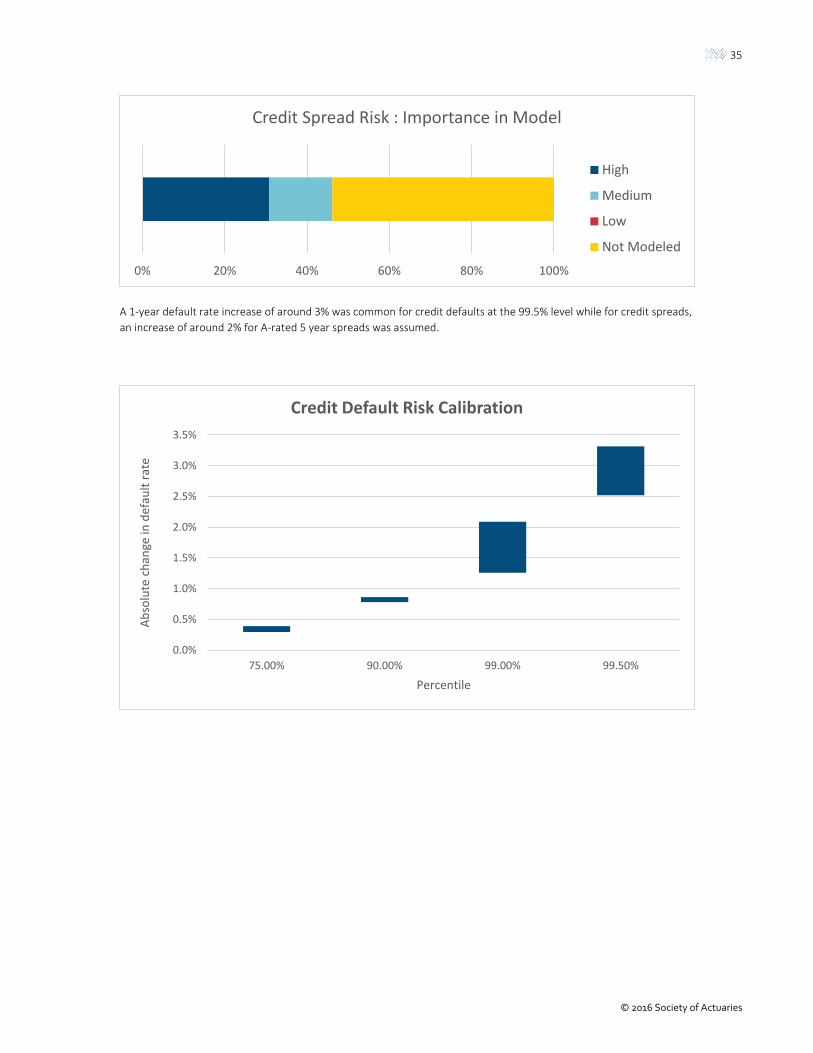
35


A 1-year default rate increase of around 3% was common for credit defaults at the 99.5% level while for credit spreads,

an increase of around 2% for A-rated 5 year spreads was assumed.

0% 20% 40% 60% 80% 100%

Credit Spread Risk : Importance in Model

High

Medium

Low

Not Modeled

0.0%

0.5%

1.0%

1.5%

2.0%

2.5%

3.0%

3.5%

75.00% 90.00% 99.00% 99.50%

Ab

solu

te c

han

ge in

def

ault

rat

e

Percentile

Credit Default Risk Calibration

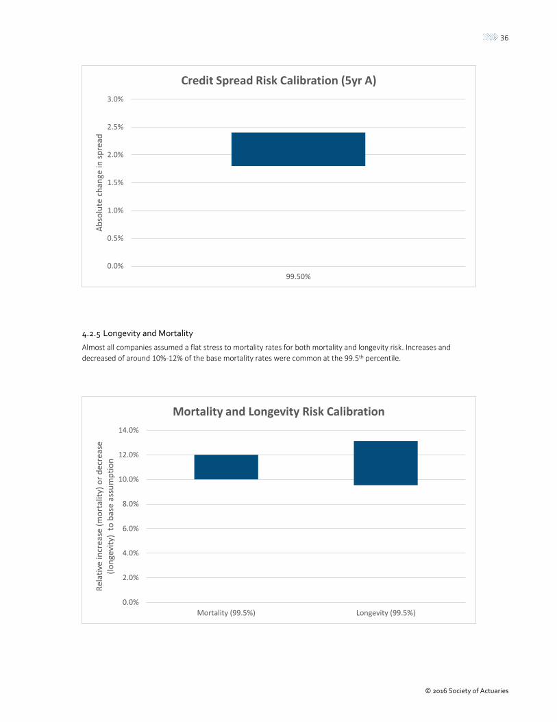
36


4.2.5 Longevity and Mortality

Almost all companies assumed a flat stress to mortality rates for both mortality and longevity risk. Increases and

decreased of around 10%-12% of the base mortality rates were common at the 99.5th percentile.

0.0%

0.5%

1.0%

1.5%

2.0%

2.5%

3.0%

99.50%

Ab

solu

te c

han

ge in

sp

read

Credit Spread Risk Calibration (5yr A)

0.0%

2.0%

4.0%

6.0%

8.0%

10.0%

12.0%

14.0%

Mortality (99.5%) Longevity (99.5%)

Rel

ativ

e in

crea

se (

mo

rtal

ity)

or

dec

reas

e (l

on

gevi

ty)

to

bas

e as

sum

pti

on

Mortality and Longevity Risk Calibration

37


Where companies modelled mortality improvements, an increase (or decrease) in improvement rates of between 0.5%

and 0.75% was assumed. Values in the charts below show the absolute value of assumptions provided. Slightly higher

improvement rates for older ages were assumed by some respondents.

Median excess deaths of around 14 per 10,000 lives were assumed for a mortality catastrophe at the 99.5% level.

Where lapse rates were stressed, this was generally applied as a percentage increase to base lapse rates. At the 99.5%

level this was typically around a 25% increase. Many companies reported using dynamic lapse stresses instead of or in

addition to these lapse factors which did not have simple quantification and / or varied by product type.

0.0%

0.2%

0.4%

0.6%

0.8%

99.50%

Ab

solu

te a

dd

itio

nal

imp

rove

men

t

Mortality Improvement Risk Calibration (Male Age 50)

0.00%

0.05%

0.10%

0.15%

0.20%

99.50%

Percentile

Mortality Catastrophe Risk Calibration

38


Companies stressing expenses generally applied expert judgement to derive the stress levels. Most experts agreed that

around a 10% increase in expenses was correct.

. . .

0.0%

5.0%

10.0%

15.0%

20.0%

25.0%

30.0%

99.50%

Rel

ativ

e ch

ange

in b

ase

lap

se r

ates

Percentile

Lapse Risk Calibration

10.2%

10.3%

10.4%

10.5%

10.6%

10.7%

10.8%

10.9%

11.0%

11.1%

99.5%

Rel

ativ

e ch

ange

in u

nit

exp

ense

s

Percentile

Expense Risk Calibration

39


Section 5: Influence of Market and Supervisory Developments

As economic capital models are primarily designed to follow useful and realistic economic principles, they need not

strictly follow the frameworks promoted by solvency regulation or supervisory bodies. Nonetheless, market and

supervisory developments have an important influence on EC developments, for example, several European insurers

seek to develop internal EC models that qualify for equivalence under Solvency II regulation.

This section of the report is designed as an introduction to some of the most relevant developments, focusing

specifically on their influence to EC practitioners. The details of these developments are expected to evolve over time;

therefore, this section, which was initially drafted in 2015, may go out of date more quickly than other sections of this

report, and readers who are interested in detailed supervisory guidance should consult the relevant regulator or

supervisory authority identified below.

5.1 Global Financial Crisis

Much has been written about the causes and effects of the global financial crisis of 2008. Despite a few notable

struggles by major insurance groups, it is generally believed that the insurance industry suffered less—at least in the

immediate aftermath—than the banking industry, largely attributable to the fact that short-term liquidity is less critical

for long-term insurance products. Insurers also were not as heavily invested in the subprime mortgaged-backed

financial instruments that led to large scale write-downs by financial institutions.

However, this is not to say insurers did not feel the effects of the financial crisis. In the years following the initial crisis,

the general economic slowdown and low interest rate environment put a strain on insurance products, as insurers

struggled to fund embedded guarantees and crediting rates amidst realized and unrealized investment losses. Having

observed potential adverse outcomes on both the asset and the liability side of the balance sheet, risk managers grew

skeptical of the ability of most regulatory models to adequately reflect complex risk profiles. Insurers also came to

realize their pre-2008 EC models were not adequately designed to meet the demands of risk management. The

importance of frequent sensitivity testing and solvency monitoring has been a major driver in subsequent

developments, using techniques and methodology considerations described throughout this report.

The global financial crisis also led to the development of new supervisory frameworks in local and international

jurisdictions. The following sections provide high level overviews of some of those frameworks in terms of their

influence on EC development. They are not meant to provide detailed supervisory guidance, which is beyond the scope

of this report.

5.2 Solvency II

The Solvency II Directive provides a major update to solvency regulations for European insurers. Implemented January

1, 2016 but under lengthy development for many years leading up to the effective date, insurance practitioners around

the globe watched the details unfold and worked to remain informed of the requirements and rationale. As a group-

wide initiative, Solvency II has an impact not just on European domestic insurers, but also on any subsidiary with a

European parent or any company wishing to explore the competitive landscape in Europe. The high-profile nature of

the development and testing phases caused rating agencies and regulators to take note even if they were not directly

impacted, and several European and non-European insurers used this as an opportunity to explore how their risk

management practices aligned with qualitative and quantitative recommendations.

The economic capital measurement under Solvency II is based on a 1-year risk approach targeting a 99.5th percentile

(although some flexibility is afforded to internal model companies), and indeed, many EC models around the world now

reflect similar approaches whether or not they are used for Solvency II reporting .

40


Solvency II is based on a market value of assets and market-consistent value of liabilities measure, with risk assessed

over a 1 year timeframe. However, numerous adjustments to true market-consistent valuation of liabilities are used.

These include material adjustments to the risk-free yield curve in the form of the matching adjustment and volatility

adjustment, and an extrapolation of the risk free yield curve at longer durations.

Solvency II also introduced the concept of an “internal model,” which allows for principles-based development of a

capital model subject to a rigorous regulatory approval process. This concept has contributed to a modeling spectrum

ranging from regulatory prescribed capital to internal economic capital, partly blurring the boundary between the two.

Other regulatory regimes are at least following suit with various principles-based initiatives under exploration.

5.3 Own Risk and Solvency Assessment

The Own Risk and Solvency Assessment (ORSA) is a regulatory requirement for insurers to self-assess their risk and

solvency position, generally on an annual basis. Guidelines in the U.S. are defined by the National Association of

Insurance Commissioners (NAIC), and similar requirements are coming into effect in most major insurance markets

around the globe.

Quantitative aspects of the ORSA include an assessment of risk exposure and a projection of future capital needs under

normal and stressed environments. As of the writing of this paper, many U.S. insurers are preparing their first ORSA

filing and are consequently relying on existing models—including those used for regulatory cash flow testing, GAAP

accounting, or economic capital—as they establish processes to meet the reporting requirements. In many cases,

insurers are finding that existing actuarial models do a good job of projecting cash flows (as they were designed to do)

but are limited in their ability to project capital requirements, which involves a more complex distribution of possible

scenarios to account for risk in the tail. Due to the emphasis on the ‘O’ in ORSA, which gives insurers flexibility to

perform these assessments according to internally relevant metrics and valuation bases, the use of EC is likely to

continue growing for this purpose.

5.4 Global Capital Standards

Largely driven by the International Association of Insurance Supervisors (IAIS), global capital initiatives are currently

underway to promote solvency among large insurance groups designated as Global Systemically important Insurers (G-

SIIs) or Internationally Active Insurance Groups (IAIGs).

Requirements for G-SIIs include the Basic Capital Requirement (BCR). Sharing fundamental similarities to the NAIC Risk-

Based Capital framework (RBC), the BCR is a factor-based calculation, in which capital requirements are determined by

prescribed factors applied to certain measurements of size, varying by product. The most notable departure from RBC

is the use of a “current estimate,” as opposed to book value, for measuring some types of liability values, which may

influence the selection of an underlying valuation basis for EC models. Though it is too early to tell how pervasive the

BCR’s influence will be, the simplistic nature of the calculation, the limited number of G-SIIs to which the BCR is applied,

and the IAIS’s indication that the BCR may be a temporary measure all suggest this will not significantly influence EC

methodology for most insurers.

Requirements for IAIGs will include the Insurance Capital Standard (ICS). As of the writing of this report, the ICS is in the

early stages of development, and several methodology options are being explored. A one-year risk horizon seems to be

a tentative option, reflecting the influence of Solvency II, and both GAAP and market value measurements have been

proposed as the basis for valuations. Again, it is too early to tell if the ICS will be implemented as planned or how

influential it will be, but the intended application to internationally active groups suggests many insurers (whether or

not they are designated IAIGs) may consider adopting all or parts of the ICS calculation into their EC frameworks.

41


5.5 U.S. Federal Regulatory Activities

In the U.S., the Dodd-Frank Wall Street Reform and Consumer Protection Act (more simply known as Dodd-Frank) gives

authority to the Financial Stability Oversight Council (FSOC) to identify and monitor risks to the financial system. As part

of this undertaking, FSOC is responsible for identifying Systemically Important Financial Institutions (SIFIs), who are

then subject to requirements including the Comprehensive Capital Analysis and Review (CCAR). Though most

commonly associated with banks, the SIFI scope spans non-banking institutions, including insurers.

CCAR requirements include a series of stress tests to determine capital adequacy under possible future economic

scenarios. Both base and adverse scenarios are included; however, there are only five scenarios in total. For this

reason, CCAR is useful for supplemental risk analysis, but it lacks the ability to attribute risk to individual risk drivers or

the interactions between them, which would be required for many of the EC applications discussed in Section 6.

Therefore, it is unlikely to have a strong influence on the development of EC models.

42


Section 6: Applications of Economic Capital

Implementation of EC will only add value to an insurer if it is used effectively within business operations. Business

utilization of EC is a requirement for some regulatory regimes (e.g., Solvency II internal models), and additionally, many

insurers are choosing to emphasize such use in their rating agency reviews and ORSA summary reports, and indeed,

S&Ps Level III review requires insurers to pass the use test. Most generally, EC has direct applications as a risk

management tool designed to better inform strategic decision for insurers. The principal areas in which EC can be used

in this way are considered below.

6.1 Capital Adequacy

Capital adequacy is the core use of EC for most insurers—providing a measure of capital that truly captures the risk of

the insurer’s own portfolio, free from the distortions of regulatory reserving and capital requirements and the

simplified approximations within most rating agency models.

Effective use of EC in measuring capital adequacy requires the EC measure to be integrated into the capital

management process, with potential EC requirements along a number of scenario paths being developed and capital

funding strategies developed to address these. Strategies also need to be developed for addressing fluctuations in

experience over time, which will result in variations in the difference between actual capital held and the EC

requirement. Typically actual capital is targeted to remain within a band based on the EC calculation, with action being

taken if EC falls outside this band—either to raise or refund capital or to modify the risk profile of the company to align

it better with the available capital.

Acceptance of the EC calculations by regulators and rating agencies is necessary for achieving its business benefits, and

EC often features strongly in discussions on capital adequacy with these third parties. The EC results would usually only

be presented at a high level—perhaps for the company overall or by major business segment—but there would also be

a discussion of the underlying methodology, models and assumptions, with the company explaining clearly why the

approach and results appropriately reflect the underlying risk profile of the company. EC also often plays a significant

role in presentations to shareholders and investment analysts, typically as part of the insurer’s overall risk and financial

management framework

6.2 Capital Allocation

Target capital levels are often defined and calculated at an aggregate level. To facilitate management against these

targets, it is necessary to allocate these capital amounts down to more granular levels of the business or risk drivers. A

desirable property for capital allocation methods is additivity, such that if each line of business is holding their exact

allocated amounts of target capital, then the enterprise is also operating at its target level, which requires in particular

a mechanism for allocating diversification benefits. Since diversification is a property of interactions between different

risks or lines of business, decisions must be made to identify the best mechanism to achieve this, and in practice, two

methods have emerged as most common within the life insurance industry:

Pro-rata allocation involves allocating total diversified capital (or diversification benefits) in proportion to

standalone capital amounts. This is the simplest method to implement and, unlike some other approaches, does

not require the use of stochastic scenarios; however, it implicitly assumes that all lines of business have similar risk

profiles and may therefore distort results whenever this is not true.

Euler allocation starts from diversified capital calculated at the aggregate level and identifies a range of scenarios

that produce a similar loss amount. These scenarios could be significantly different (e.g., a large equity fall or a

global pandemic could each reduce available surplus to near zero), and in the presence of Monte Carlo simulation

models, a large number of such scenarios could exist. The technique is then to take an average across each of

these scenarios to identify the risk drivers or loss amounts corresponding to more granular levels, possibly with a

43


minor scaling adjustment to ensure additivity is preserved. This approach ties allocated amounts directly to risk

profiles, and for this reason it has grown in popularity over recent years. The disadvantage is that a large number

of simulations may be required, and negative capital amounts might be allocated to low risk parts of the business,

which can be challenging to explain.

6.3 Risk Appetite

EC is a key measure of risk from a policyholder perspective and therefore frequently features as an important

component of an insurer’s risk appetite framework and in the monitoring processes implemented to ensure the insurer

remains within that risk appetite. To do this, target ranges (including, in particular, upper limits) for EC utilization need

to be established for each geography, business unit and/or risk, and actual EC monitored against these target ranges

(e.g., by way of a risk dashboard). The setting of such ranges and limits needs to take into account the expected level of

diversification between risks as well as the level of granularity. For example, to the extent that limits are set for legal

entities that have restrictions on capital transfers, the limits should be reviewed in total to ensure they are still aligned

with company tolerances.

Use of EC for this purpose requires an ability to update EC (and available capital) on a frequent basis to reflect the

changing risk profile of the organization. For insurers with a very rapidly changing risk profile, this potentially implies

daily or weekly updating for market risk movements, albeit with some approximation likely.

EC may also play a role alongside broader capital objectives, with multiple tiers of capital held to meet higher order

needs. For example, the first tier may serve to protect policyholders’ benefits, with subsequent tiers aiming to maintain

credit ratings, then to establish buffers to ensure regulatory compliance for reserves and capital, and so on. Two

examples of such a multi-tiered objective statement might be:

Capital tier / objective order

Example 1 Example 2

1 Meet policyholder cash flows as they fall due with a 95% certainty over the life of the business

Meet policyholder cash flows as they fall due with a 95% certainty over the life of the business

2 Meet debt payments as they fall due with a 90% certainty

Maintain capital to support or exceed current rating level with a 90% certainty

3 Ensure regulatory capital ratio above 200% with a 90% certainty over the next 5 years

Ensure objective 2 is met with an 80% certainty over the next 5 years

. . . In the first example the company takes a regulatory view of meeting requirements – ensuring they comply with a

high certainty with all requirements. In the seconds the company takes an economic view of requirements, ensuring

they will be well capitalized on their internal EC basis even under stress conditions.

The level of certainty that is desired for each objective depends on balancing the costs of failure and the cost of

retaining extra capital. Capital above the regulatory minimum required is therefore held to protect or enhance the

interests of a number of stakeholders and to increase shareholder returns by avoiding the costs of failure to meet the

company’s objectives. Conversely, holding higher levels of capital can be seen as having a cost for the business relating

to tax, investment costs and potentially agency effects, thus reducing shareholder value. Additional capital also reduces

the value of the “shareholder put option”—the shareholders’ rights to walk away from the company once its liabilities

44


exceed its assets. Using a model of the costs of failure, an expected return on capital to shareholders can be found and

optimized.

In order to assess the amount of capital required under this multi-tiered definition, relatively sophisticated models are

required. For example, risks could be projected over the life of the existing policies in a number of scenarios forming a

real world distribution. At each future time step in the projection, asset and liability cash flows would be produced,

possibly along with reserve valuations and regulatory capital requirements. The shortfall in each period is then

assessed, and the capital requirement is identified to eliminate the shortfall with some certainty for each of the

objectives. The company’s business model may also necessitate adjustments to this approach. For example, a company

with a sizeable hedging program may have corresponding market risk and liquidity risk, reducing the focus on cash

flows and increasing the focus on default risk.

These considerations support a view of capital which is more complex than protecting policy benefit payments. In this

view, capital can be thought of as having a hierarchy of utility at increasing amounts. These tiers are specific to each

company and should relate closely to their business objectives and operating environment. Each tier should have a

specific trigger and objective for the company. The complexity of this structure can grow quickly; therefore,

establishment of EC models is an important foundational step.

6.4 Performance Measurement

Improved performance measurement is a commonly cited reason given by companies for wanting to calculate EC. In

broad terms, a higher level of EC for one business unit compared to another signifies a higher level of risk and

therefore suggests that a higher level of reward should be expected. At a more detailed level, however, insurers are

exposed to risks of many types, with the balance varying significantly between business units, and it is generally

accepted that the appropriate level of reward for risk varies by the nature of that risk. In particular, diversifiable risks

attract lower returns than those that cannot be diversified (often referred to as systematic risks).

It is important to note that by itself, EC does not represent a measure of business performance, but rather gives a

measure of the risk related to the business. In order to use EC to measure performance, it needs to be incorporated in,

or combined with, some related measure of return. In practice there are two broad approaches adopted by companies

when using EC in performance measurement.

One approach involves calculating a return on capital, using EC as the (risk-adjusted) capital measure in the

denominator of the calculation. This is a measure of Return on Risk-Adjusted Capital (RORAC). Consideration then

needs to be given to the appropriate measure of return to be used in the formula and whether this also needs to be

risk adjusted (taking into account the nature of the risks in each business segment). The measure of return used will

have a critical impact on the results and on the relative perception of different business units. A true economic

measure of performance requires an economic return to be used. In practice non-economic measures such as GAAP

earnings are sometimes used as the “return” in the formula; the potential impact this might have on results (compared

to an economic return) should, however, be carefully considered before following this route.

An alternative approach to measuring performance on a risk-adjusted basis involves the inclusion of EC as the measure

of required capital within a value-based measure, such as embedded value (EV). Companies calculating EV are

increasingly using EC for this purpose rather than statutory or rating agency based capital.

The EC-based performance measures mentioned above are also starting to be used in incentive compensation

schemes, although this has not been that common to date. Indeed this can in many respects be considered the critical

test as to whether EC, and ERM more generally, is fully embedded within the business. Given the push from rating

agencies and regulators for such embedding of EC, it seems likely that risk-adjusted measures will increasingly become

part of the incentive compensation structure of insurers.

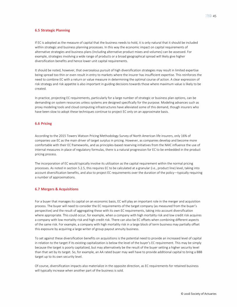
45


6.5 Strategic Planning

If EC is adopted as the measure of capital that the business needs to hold, it is only natural that it should be included

within strategic and business planning processes. In this way the economic impact on capital requirements of

alternative strategies and business plans (including alternative product mixes and volumes) can be assessed. For

example, strategies involving a wide range of products or a broad geographical spread will likely give higher

diversification benefits and hence lower unit capital requirements.

It should be noted, however, that overzealous pursuit of high diversification strategies may result in limited expertise

being spread too thin or even result in entry to markets where the insurer has insufficient expertise. This reinforces the

need to combine EC with a return or value measure in determining the optimal course of action. A clear expression of

risk strategy and risk appetite is also important in guiding decisions towards those where maximum value is likely to be

created.

In practice, projecting EC requirements, particularly for a large number of strategic or business plan options, can be

demanding on system resources unless systems are designed specifically for the purpose. Modeling advances such as

proxy modeling tools and cloud computing infrastructures have alleviated some of this demand, though insurers who

have been slow to adopt these techniques continue to project EC only on an approximate basis.

6.6 Pricing

According to the 2015 Towers Watson Pricing Methodology Survey of North American life insurers, only 16% of

companies use EC as the main driver of target surplus in pricing. However, as companies develop and become more

comfortable with their EC frameworks, and as principles-based reserving initiatives from the NAIC influence the use of

internal measures in place of regulatory formulas, there is a natural progression for EC to be embedded in the product

pricing process.

The incorporation of EC would typically involve its utilization as the capital requirement within the normal pricing

processes. As noted in section 5.2.5, this requires EC to be calculated at a granular (i.e., product line) level, taking into

account diversification benefits, and also to project EC requirements over the duration of the policy—typically requiring

a number of approximations.

6.7 Mergers & Acquisitions

For a buyer that manages its capital on an economic basis, EC will play an important role in the merger and acquisition

process. The buyer will need to consider the EC requirements of the target company (as measured from the buyer’s

perspective) and the result of aggregating these with its own EC requirements, taking into account diversification

where appropriate. This could occur, for example, when a company with high mortality risk and low credit risk acquires

a company with low mortality risk and high credit risk. There can also be EC offsets when combining different aspects

of the same risk. For example, a company with high mortality risk in a large block of term business may partially offset

this exposure by acquiring a large writer of group payout annuity business.

To set against these diversification benefits on acquisitions is the potential need to provide an increased level of capital

in relation to the target if its existing capitalization is below the level of the buyer’s EC requirement. This may be simply

because the target is poorly capitalized, but may alternatively be the result of the buyer setting a higher security level

than that set by its target. So, for example, an AA rated buyer may well have to provide additional capital to bring a BBB

target up to its own security level.

Of course, diversification impacts also materialize in the opposite direction, as EC requirements for retained business

will typically increase when another part of the business is sold.

46


Section 7: Implementation and Communication

7.1 Objectives

An insurer’s objectives for calculating EC, including how the results are to be used in the business, will have an

important influence on the appropriate implementation approach, most notably on the level of detail and frequency of

the calculation. It is likely that trade-offs will need to be made, for example, between the accuracy of the EC results and

the timeliness of their availability for business utilization.

7.1.1 Capital Adequacy

When EC is primarily used for capital adequacy, there is less pressure to present results at detailed levels and a greater

focus on group or entity level results. This can allow a less granular approach to modelling, including removing the need

to allocate asset pools to liability blocks. Following this route can however, lead to difficulties in understanding and

validating results. Because there will often be a need to discuss the capital adequacy results at Board meetings and

with external third parties, an approach that is easily communicated has advantages, which is one reason why VaR

metrics may be chosen over CTE in spite of the theoretical advantages of the latter.

7.1.2 Risk Management

In addition to capital adequacy, EC is an important measure of risk from a policyholder perspective and therefore

frequently plays a central role in insurer’s risk appetite framework. For this purpose, EC needs to be captured not only

at the corporate level but also at a more granular level, with the precise decomposition of EC being determined by the

insurer’s risk management structure and monitoring processes. For example, in some insurers management control of

all risks lies with the business units, whereas in others market and credit risks are managed at the corporate level, with

business units primarily being responsible for insurance and operational risks. Either way, a process for the allocation of

EC at a more granular level is normally required.

The decision to use EC to monitor and control risk at an operational level can also have significant implications for the

model design and choice of systems. EC needs to be calculated at (or allocated down to) a detailed level and needs to

be calculated at a frequency appropriate to the risk being captured. For example, weekly or daily updates may be

needed where EC is used to monitor asset/liability or hedging exposures, given the rapid pace of market movements

and the potential changes in asset exposure. Indeed, if EC is to be used to monitor the trading activities of individual

staff (including potential fraud), a link to real time asset data is likely to be needed. Advances in modeling approaches

(e.g., the use of proxy models) are permitting the direct use of EC for such purposes.

7.1.3 Performance Measurement

The use of EC for performance measurement requires a level of granularity appropriate to the performance

management framework (e.g., typically by business unit) and a frequency of calculation appropriate to the pace of

change in risk profile. In addition, there will be a strong need to demonstrate the consistency of the EC metric across

different risks and lines of business if it is to be applied uniformly, and it must be perceived as a robust and objective

measurement. These motivations can lead to a more centralized and governed process for setting parameters than

would otherwise be the case. Finally, the approach must be capable of clear explanation to the individuals affected.

47


7.1.4 Other Strategic Objectives

EC is often implemented with the objective of providing management with a better informed basis from which it can

make risk-based decisions, including hedging, reinsurance and mergers and acquisitions. For EC to be a useful tool in

this regard, companies need to ensure it can be applied at a sufficient level of granularity and determined at a

sufficient level of accuracy to be applied to the range of possible decisions with which they are, or could be, faced. For

example, an approximate approach to EC that did not reflect the full detail of asset/liability mismatches would be of

limited use in determining detailed asset strategy.

Strategic support in pricing and other decisions requires a process for allocating EC down to the product level, including

the level of diversification credit considered appropriate. It also requires the projection of the chosen (allocated)

measure of EC over the term of the products being modeled, allowing in a reasonable way for the changes in risk

profile over that term. Modeling developments have now reached a stage that feasibly allows for the direct projection

of EC metrics without limited necessity for approximations, leading to a growth in this area of practice.

7.2 Constraints

In addition to considering the primary objectives for calculating EC, insurers are often faced with resource constraints

that further influence the design of the EC framework.

A company facing budget or time constraints may opt for a less sophisticated initial approach if the implementation can

be maintained in a way that still meets the highest priority objectives. In this situation, companies often consider

phased implementations, first demonstrating the value that is achieved from the initial model, and then expanding the

model to adopt increasing sophistication over time. Ultimately, the added sophistication should lead to more accurate

and more useful results to justify the use of additional resources.

While system constraints have reduced over time, increases in computing capacity and improved systems design are

frequently matched by increased demands on the part of users (whether for more complex calculations or faster

runtimes), so system challenges may continue to constrain EC implementations. A particular issue is the potential need

to calculate a projected economic balance sheet for business with embedded optionality, either in the context of a

one-year EC time horizon or as an intermediate solvency check within a runoff approach. If a stochastic approach to EC

is adopted, this theoretically requires “stochastic on stochastic” modeling, which remains highly system intensive even

with the latest hardware and software. As a result, companies have often implemented simpler approaches to EC, such

as stress testing based approaches. These give a good indication of overall EC requirements and of the exposure to

specific risk factors, although careful thought needs to be given to how the impact of the different risk drivers is

aggregated (for example by the examination of combined risk scenarios).

The use of proxy models has emerged as a leading technique to address system constraints, and when properly

calibrated, can lead to a high degree of accuracy at significantly reduced runtime. Proxy modeling identifies polynomial

functions relating movements in risk drivers to changes in value as calculated by a full run of the asset-liability systems.

After these functions are validated, they can be used for rapid revaluation of balance sheet metrics without the need to

rerun the underlying models. These approach can be used for intermediate reporting (e.g., weekly or monthly), and

more sophisticated calculations are used periodically (e.g., semi-annually or annually) to ensure the proxy functions

remain valid.

Finally, limited availability of skilled staff can restrict an insurer’s options when embarking on an EC implementation.

This constraint may apply separately in the implementation phase and on an ongoing basis. In implementation,

companies may simply find they do not have sufficiently skilled or knowledgeable staff. On an ongoing basis, the

company may not be able to justify the cost of a dedicated EC team on a full-time basis as may be required to maintain

some of the more sophisticated EC approaches. In implementation, many companies make use of external consultants

to provide the expertise, while at the same time training the company’s staff to manage much of the process on an

ongoing basis.

48


7.3 Model Governance

Governance is a critical factor in determining the success of an EC implementation, both in the development phase as

well as on an ongoing basis as enhancements are made. Successful EC implementation involves a significant amount of

active participation and direction by senior management. With key decisions around the implementation and use of EC

being driven from the top, there is ownership and buy-in of EC at the leadership level of the organization.

On an operational level, there needs to be a clear business owner of EC, which typically falls under the responsibility of

a senior executive. This role is an important strategic one and includes providing the overall strategy and guidance on

use of EC within the organization. It should be viewed as distinct from, but related to, the role of those who physically

run the models and perform the calculations on a day-to-day basis.

In addition to senior level buy-in, buy-in across all levels of the organization is important. Generally, this is readily

achieved with effective communication coming from the senior management or even the board of directors, where

ultimate responsibility lies. Internal and external communication is integral to a successful EC implementation.

Internally, an effective top-down communication plan can help secure buy-in at all levels of the organization. The

details of the communication are typically tailored to the audience and can include topics such as the rationale for the

company’s decision to implement EC, the short-term and long-term plans for EC within the company, the overall EC

methodology, the modeling requirements and the expected involvement from the business. Training at various levels

within the organization is also considered an important aspect of internal communication. The communication of

specific information, coupled with training, can be particularly important in influencing the behavior and thinking of the

people in the business lines who will ultimately be responsible for making EC become part of the normal operations of

the business.

Bottom-up communication can also be important by giving the business managers the opportunity to react and provide

feedback to the top-down EC communication from senior management. This process may include allowing those within

the business to contribute to the development of the EC methodology and related decisions. In these situations, a

challenge for many companies can be deciding on when to involve businesses and to what extent to involve them.

In establishing the internal infrastructure and processes for implementing EC and calculating it on an ongoing basis, a

question many insurers face is to what extent the work should be maintained at the corporate level by a dedicated

ERM team versus being pushed down into business units or product owners. There are certain aspects that are typically

advantageous to remain at the centralized level. For example, setting out the high-level methodology, aggregating

results, and reporting in a consistent manner often requires a high level, centralized view to ensure consistency. In a

similar way, many insurers prefer to centrally coordinate certain risk calibration decisions, especially those related to

generating economic scenarios. In contrast, modeling decisions related to how scenarios are measured within a

product line and what type of product features must be captured are usually pushed out to local experts. Overall, these

are largely cultural decisions with a range of implementations in practice.

7.4 Validation

Validation, encompassing both the initial implementation of the model as well as its ongoing use, is critical for

obtaining confidence in the results. A validation framework often includes, but is not limited to, a review of the

following components:

Intended use of the model

Soundness of the EC methodology

Calibration of stress scenarios

Usefulness and accuracy of model outputs

Quality of documentation

Ownership, governance, change procedures and sign-off

49


EC models are often based on existing cash flow projection models used for other purposes (e.g., for calculating

embedded value), and consequently these underlying models may already have been subject to testing appropriate to

those purposes. Validation of models to be used for EC purposes, however, typically needs to be extended to include

detailed examination of results in the adverse tail of the distribution, which will be influential drivers of the EC results.

In particular, the validity of management actions (such as credited rate assumptions or asset strategy) and policyholder

behavior assumptions should be reviewed in the context of extreme scenarios being examined.

One particular aspect of validation often referred to in the context of EC implementation is the back testing of the

models against actual historical data. This is primarily used to test the calibration of the risk factor distributions and

correlation assumptions, although it can also serve as a test on other assumptions and parameters in the model. In

some cases it may not strictly be possible to fully back test an EC model due to the extreme confidence levels

involved—for example, testing a one-year approach calibrated to a 99.5% confidence level would require several

hundred years of historical data to derive meaningful results. However, even in these cases, meaningful reasonability

checks can still be performed to analyze how available experience compares to risk factor calibrations. For example, it

is fully possible that a 1-in-200 year event may have occurred within the last 50 years, so such an observation would

lead to a careful review, but not necessarily a change, of the EC assumptions; observing 10 of these events would

almost certainly lead to a change.

A thorough treatment of validation techniques is beyond the scope of this report and could be covered in an entire

report on its own. Additional details can be found in publications dedicated specifically to this topic, for example, the

North American Chief Risk Officer Council published “Model Validation Principles Applied to Risk and Capital Models in

the Insurance Industry” in December 2012.

7.5 Reporting

It is important for reporting needs to influence model development. Companies that fail to clearly define their

reporting requirements can fall into a trap where the desire for increasingly advanced calculations drives model

development, often at the cost of decreased reporting capabilities. Models can quickly grow in complexity or

granularity, and even though calculations may indeed become more accurate, this does not translate to added value if

the reports can no longer be produced on time or in a format that can be communicated effectively.

As with other types of models, the usefulness of EC depends on the ability to extract reliable and timely results. Ideally,

results should be available according to different splits of the business, aligned with how EC is used for business

applications. For example, a “risk report” might show EC results allocated to major risk categories across all lines of

business, while a “business unit report” might show EC results allocated to each line of business, then further drilled

down to unique risk drivers. Similar reports can be produced for different geographic regions and other relevant

management attributes. Early adopters of EC tended to build models that produced these results on an annual basis,

which limited the usefulness of the model. As programs have matured, they are now producing results monthly or

more frequently for certain applications, allowing management to make risk decisions in response to near-real-time

movements in the economic or business environment.

Date post:	02-Aug-2019
Category:	Documents
Upload:	hatruc
View:	216 times
Download:	0 times

Economic Capital for Life Insurance Companies - soa.org · In 2008, the Society of Actuaries (SOA)...

Documents