Page 1
Partnership for America’s Economic Success | Page 1
Economic Costs of Early
Childhood Poverty
By
Greg J. Duncan, Northwestern University
Ariel Kalil, University of Chicago
Kathleen Ziol-Guest, Harvard University
Issue Paper #4
Page 2
Partnership for America’s Economic Success | Page 2
This report is based on a paper co-authored by Greg Duncan of Northwestern University, Ariel
Kalil of the University of Chicago, and Kathleen M. Ziol-Guest of Harvard University. The
authors gratefully acknowledge the peer reviews and advice of Rucker Johnson, Michael Foster,
and Richard Wertheimer. The views expressed are those of the authors, and not necessarily
those of the reviewers, Northwestern University, the University of Chicago, Harvard University,
or The Pew Charitable Trusts.
The Partnership for America’s Economic Success was created by a group of business leaders,
economists, advocates, and a dozen funders in order to document the economic impacts to the
nation of proven investments in children from before birth to age five. The Partnership has been
funded by the Buffet Early Childhood Fund; Robert Dugger; George Gund Foundation; Horace
Hagedorn Foundation; Paul Tudor Jones; Ohio Children‟s Foundation; Peppercorn Foundation;
The Pew Charitable Trusts; PNC Financial Services Group, Inc.; Scholastic, Inc.; The Schott
Foundation for Public Education; and Anonymous. The Partnership is managed by The Pew
Charitable Trusts.
1025 F Street, NW, Suite 900 Washington, DC 20004
(202) 552-2000 | www.PartnershipforSuccess.org | [email protected]
Release Date: February 28, 2008
Page 3
Partnership for America’s Economic Success | Page 3
Contents
Executive Summary 4
Economic Costs of Early Childhood Poverty 6
Appendix on Procedures 11
References 32
Endnotes 33
Page 4
Partnership for America’s Economic Success | Page 4
Executive Summary
More than four million infants, toddlers and preschoolers lived in poverty in the United States in
2005. Our paper focuses on this question: What economic benefits would a policy provide that
brought poor children’s prenatal-through-age 5 family incomes up to the poverty line but made
no other concurrent changes in the socioeconomic status of those children’s families?
We first calculate simple differences in a number of adult outcomes between individuals whose
early childhood incomes were below, close to and well above the poverty line. Relative to
children with early childhood incomes exceeding at least twice the poverty line, poor children
complete nearly two fewer years of schooling, work 25% fewer hours, earn only about half as
much, receive $750 more per year in food stamps, and are more than twice as likely to report
poor overall health or high levels of psychological distress. Poor males are nearly twice as likely
to be arrested, and their rates of incarceration are three times as high, as those of males in higher-
income families. For females, early poverty is associated with a nearly $200 increase in annual
cash assistance from the AFDC or TANF programs and a five-fold increase in the likelihood of
bearing a child out of wedlock prior to age 21.
We next attempt to estimate the causal connections between early poverty and these adult
outcomes and find that links between early childhood poverty and five outcomes – completed
schooling, labor-market hours and earnings, and receipt of income from both the food stamp and
AFDC/TANF cash assistance programs – proved strong enough to pass our rigorous statistical
tests.
In the case of adult work and earnings, we estimate that eliminating poverty in early
childhood (through annual income transfers that average $4,326 between the prenatal
year and age 5 and bring poor children‟s family income just up to the poverty line) would
boost annual work hours by 12.4% percent and earnings by 28.7% percent per year. In
dollar terms, this amounts to lifetime earnings increases of between $53,000 and
$100,000 per child, depending on the assumed duration of the poverty effect.
Bringing poor children up to 150% of the poverty line from their prenatal year to age
5 would cost $7,066 per year, and would increase lifetime earnings by between
$105,000 and $193,000, again, depending on the assumed duration of the poverty effect.
Nationally, there are roughly 4 million young adults of any given age. With 366,800 of
them estimated to have spent their early childhoods in poverty, the aggregate earnings
benefit of eliminating poverty from the prenatal year through age 5 for children
born each year amounts to between $20 billion and $36 billion.
In the case of food stamps, we estimate that eliminating poverty in early childhood would
reduce lifetime food stamp receipt in adulthood by at least $1,600. For cash assistance
from the old AFDC or newer TANF programs, eliminating early poverty for females is
estimated to lead to lifetime reductions of at least $1,250. These translate into
aggregate taxpayer saving of between $590 million and $230 million for eliminating
poverty from the prenatal year through age 5 for children born each year.
Page 5
Partnership for America’s Economic Success | Page 5
In the case of education, we estimate that eliminating poverty in early childhood would
boost completed schooling by about one-fifth of a year. Some of the financial benefits of
this boost are reflected in the earning increases and reductions in cash assistance
described above. The dollar value of a number of other likely benefits – such as greater
civic involvement, or, for children, the happiness of spending childhood in a non-poor
household – is difficult to quantify.
From a taxpayer perspective, eliminating poverty from the prenatal year through age 5
provides three measureable benefits: more tax revenue (between $10,600 and $20,000 per
poor child), and fewer expenditures on food stamps ($2,000 per poor child) and cash
welfare ($1,600 per poor female child).
Page 6
Partnership for America’s Economic Success | Page 6
Economic Costs of Early Childhood Poverty
Some 4.1 million infants, toddlers and preschoolers lived in poverty in the United States in 2005.
For a family of three, this meant that total income was less than $15,577; many poor families had
income well below that amount.1 Ample research shows that, relative to non-poor children, poor
children will be less successful in school and, as adults, in the labor market; have poorer health;
and be more likely to commit crimes and engage in other forms of problem behavior.2 Despite
these associations, it is far from clear to what extent poverty itself is the cause of these
differences. Our paper focuses on estimates of the long-run impacts of low income early in life,
net of correlated family factors. Specifically, our policy question is: What economic benefits
would a policy provide that brought poor children’s prenatal-to-age 5 family incomes up to the
poverty line but made no other concurrent changes in the socioeconomic status of those
children’s families?
The potential for detrimental impacts from early childhood poverty is obvious. Emerging
evidence from human and animal studies highlights the critical importance of infancy and early
childhood for brain development and for setting in place the structures that will shape future
cognitive, social, and emotional outcomes.3 Poverty and its attendant stressors have the potential
to shape the neurobiology of the developing child in powerful ways, which may lead directly to
poorer physical and mental health later in life. Poverty in early childhood can also reduce
material investments in children‟s learning and development, as well as interfere with the
development of strong parent-child bonds and supportive parenting practices. Such a lack of
material and emotional resources in the family environment can compound and amplify the
neurobiological disadvantages that many poor children already face. The sensitivity of early
childhood to environmental influences has been demonstrated in a wide range of infant, toddler,
and preschooler intervention studies. Taken together, they show that early-life interventions may
well be the most effective and cost-efficient approaches to promoting human capital
development.4
Our study draws on national data from the Panel Study of Income Dynamics (PSID) to estimate
linkages between income early in childhood and later life outcomes. The PSID is the longest-
running longitudinal study of household income in the United States and offers detailed
economic and demographic information across the life course. Ours is the first study to link
high-quality income data across the entire childhood period with adult outcomes measured as
late as age 37.
Our strategy is to measure income in every year of a child‟s life from the prenatal period through
age 15, distinguishing income early in life (prenatal through 5th
year) from income in middle
childhood and adolescence. Our analyses relate an array of adult achievement, social assistance,
health and behavior measures to these childhood stage-specific measures of income, plus a host
of relevant control variables. The adult outcomes we consider include educational attainment,
earnings, work hours, receipt of food stamps and cash assistance, non-marital childbearing,
crime, and mental and physical health. With details provided in an appendix, our approach
employs the following procedures.
Page 7
Partnership for America’s Economic Success | Page 7
Adult outcomes that might be linked to childhood poverty
We examine impacts of early childhood poverty on a diverse set of adult achievements,
behaviors and health conditions, all of which either add to the productive capacity of the nation
or drain its resources. As reflected by completed schooling, work hours, and earned income, the
productivity of workers is an obvious economic component of adult attainment. Poverty early in
childhood may hinder the acquisition of formal schooling and job-related skills, reduce labor-
market productivity, and limit a worker‟s access to high-wage jobs.
Behaviors that impose notable costs on society include crime and teen non-marital childbearing,
so we also estimate impacts of early poverty on arrests and incarceration for males and, for
females, the likelihood of a non-marital birth prior to age 21.
Poor job skills, limited participation in the labor market, and early childbearing may increase the
likelihood and amount of public assistance receipt from programs like food stamps and
AFDC/TANF cash assistance programs.
Poor physical and mental health can also drain society‟s resources, partly by reducing its
potential productivity (which should be reflected in part by lower earnings), but also through the
costs to the healthcare system of treating such health problems. Accordingly, we estimate the
impacts of poverty early in life on poor overall health, as well as on the likelihood of showing
high levels of psychological distress in adulthood.
Linking early childhood poverty to adult outcomes
Figure 1 shows striking differences in these outcomes, depending on whether childhood income
prior to age 6 was below, close to, or well above the poverty line. Compared with children whose
families had incomes of at least twice the poverty line during their early childhood, poor children
complete two fewer years of schooling, work 424 fewer hours per year, earn about half as much,
receive $750 per year more in food stamps as adults, and are about twice as likely to report poor
overall health or high levels of psychological distress. Poor males are more than twice as likely
to be arrested and have rates of incarceration that are two times as high as those of males in
higher-income families. For females, poverty is associated with a nearly $200 annual increase in
cash assistance and a six-fold increase in the likelihood of bearing a child out of wedlock prior to
age 21.
The strong associations between poverty and adult outcomes shown in Figure 1 do not prove that
early poverty itself is the cause of these differences. Perhaps family economic conditions later in
childhood are what really matter. Or perhaps some third factor, such as inadequate parental
education, is the cause of family poverty as well as lower child achievement, worse behavior,
and poorer health. If so, then eliminating early childhood poverty, but failing to boost parental
schooling, would not improve the life chances of the children concerned. We employ statistical
techniques to account for as many confounding factors as possible in order to isolate the impact
of early poverty itself.
Our statistical models relate the adult achievement, behavior, and health measures to a given
child‟s average family income between conception and age 5. We express the estimated impacts
as improvement in adult outcomes that would result from increasing poor children‟s family
Page 8
Partnership for America’s Economic Success | Page 8
income by $4,326 per year between the prenatal year and age 5. The $4,326 figure is chosen
because, as explained below, it is the annual increase in income we estimate to be required to
bring poor children‟s early childhood income up to the poverty line. We also estimate benefits
associated with increasing income to 150% of the poverty line, which would require annual
expenditures of $7,066 per family.
As shown in Table 1, the links between early childhood poverty and five outcomes – completed
schooling, labor-market hours and earnings, receipt of food stamps, and, for females, receipt of
cash assistance – proved strong enough to pass our rigorous statistical tests. For most of the
remaining outcomes, increases in early childhood income were estimated to be beneficial, but the
magnitudes of the effects were not large enough for us to be confident that they were real.
How important are the earnings and public assistance impacts? Closing the early-childhood
poverty gap is estimated to increase adult labor market earnings by 29%, potentially quite an
important increase in long-run earnings. As shown in Table 1, the average earnings of adults
whose early childhoods are spent in families with incomes below the poverty line amount to
$17,115; 28.7% of that figure is $4,919. With that increase sustained over the 13 years between
age 25 and 37, the increment to lifetime earnings is over $63,000. If sustained over a 30-year
working life, the increment is nearly $150,000. Several refinements of this estimate are required,
some of which would result in these simple calculations overstating the lifetime earnings impact
and others of which would lead to underestimates. As explained in the appendix, we estimate
the total value of the earnings impacts to range between $53,000 (if, as appears likely, it is
sustained between ages 25 and 37) and $100,000 (if sustained through age 54).
Nationally, there are roughly four million young adults of any given age. With 366,800 (9.1%) of
them estimated to have spent their early childhoods in poverty, the aggregate earnings benefit
of eliminating poverty from the prenatal year through age 5 for children born each year
amounts to between $20 billion and $36 billion.
In the case of public assistance, we estimate that eliminating poverty in early childhood would
reduce the value amount of food stamps received by $1,600. For cash assistance from the
AFDC/TANF program, the reduction for females is estimated to be $1,200 per year. This
translates into reductions of $590 million and $230 million, respectively, for poor children
born each year.
Page 9
Partnership for America’s Economic Success | Page 9
Figure 1: Early adult attainments, program participation, health, and
behavior by poverty status between the prenatal year and age 5
0
10
20
30
40
50
60
Years of
completed
schooling
Earnings
(in 1000
dollars)
Work hours
(in 1000
hours)
Food stamps
(in 100
dollars)
AFDC/TANF
(in 100
dollars)
females
Poor health High
psychological
distress
Ever arrested
(males)
Ever
incarcerated
(males)
Non-marital
birth prior to
age 21
(females)
Mean
or
Perc
en
t
Below the poverty line Close to the poverty line Well above the poverty line
Note: “Close to the poverty line” includes average cash incomes 1-2 times the poverty line. “Well above the poverty line” includes
incomes that averaged at least twice the poverty line. In 2005, the poverty line for a family of three was $15,736.
Page 10
Partnership for America’s Economic Success | Page 10
Table 1: Impacts of Additional Income on Adult Outcomes for Children Who Are Poor When They are Young
We estimate that it would take $4,326 per year to eliminate early childhood poverty
An added $4,326 of annual income prior to age six…
is estimated to change outcomes for poor
children from…
to…
Years of schooling completed 11.8 years 12.0 years, or an increase of .18 years
Annual earnings $17,115 $22,027 or an increase of 29%
Annual work hours 1,512 hours 1,700 or an increase of 12%
Food stamps $810 $666 or a decrease of 18%
AFDC/TANF (females only) $231 $87 or a decrease of 62%
Percent with “fair” or “poor”
overall health
12.9% 10.8%, a non-significant change
Percent with high levels of
psychological distress
6.0% 4.0%, a non-significant change
Percent ever arrested (males
only)
28.1% 28.2%, a non-significant change
Percent with non-marital birth
before age 21 (females only)
52.4% 52.4%, a non-significant change
Note: “non-significant” indicates that we could not be confident that the estimated relationship between the added income and the
change in the given outcome was different from zero.
Page 11
Partnership for America’s Economic Success | Page 11
Appendix on Procedures
We sought to estimate the influence of low family income prior to school entry on children‟s
adult achievement, health and behavior. To secure these estimates, we used 1968-2005 data from
the Panel Study of Income Dynamics (PSID), which has followed a nationally-representative
sample of families and their children since 1968 (http://psidonline.isr.umich.edu/). Our general
strategy was to select children observed in the PSID between the prenatal year and at least age
21, use the PSID‟s careful annual measurements of family income to compute average income
during both the early (prior to age six) and later periods of childhood, and then relate childhood
income to the children‟s adult earnings, completed schooling, crime, non-marital childbearing,
physical health, and mental health.
Sample
We selected all PSID sample individuals who were tracked in the annual interviews between
their prenatal year and at least age 21. Drawing on PSID interviewing waves 1968-2005, this
amounted to the eight cohorts born between 1968 and 1975. We required these individuals to be
in response families in at least 12 of the 17 years from the prenatal period to age 15. Additional
sample restrictions varied along with the dependent variable. In the case of completed schooling,
we required that completed schooling be observed when the individual was 25 or older. In the
case of crime, information about the individual had to have been gathered in 1995, the year in
which crime questions were asked. In the case of earnings, work hours, and program assistance
the individual had to have been observed at least once after age 25. In the case of physical
health, information about the general health of the individual had to have been gathered at age 21
or later. In the case of mental health, the individual had to have responded to the 2003 interview
wave questions on psychological distress.
Childhood Income
We used the PSID‟s edited measure of annual total family income, inflated to 2005 levels using
the Consumer Price Index. To adjust for the time value of money, we further discounted all
income amounts to the child‟s birth year, using a discount rate of 3%. We averaged these annual
income measures across three periods: the prenatal year5 through the calendar years in which the
child turned 5; ages 6-10; and ages 11-15. To account for a differential impact of increments to
low as opposed to higher family income, we allowed the coefficients on average income within
each childhood period to have distinct linear effects for average incomes up to $25,000 and for
incomes $25,000 and higher.
Adult Outcomes
Dependent variables in our analyses spanned achievement, health, and behavioral domains. The
adult work hours and natural logarithm of the child‟s adult earnings was gleaned from all
available reports of annual earned income and work hours reported by or for the child when the
child was age 25 or older. As with childhood income, we inflated the dollar values of earnings to
2005 price levels using the Consumer Price Index (CPI) and discounted all earnings amounts to
Page 12
Partnership for America’s Economic Success | Page 12
age 25, using a discount rate of 3%. To adjust for age and calendar year effects, we regressed all
of these earnings observations, including those reporting zero earnings, on age and calendar year
dummies, obtained residuals, and then used the sum of the residuals and the overall sample mean
earnings, averaged across all available years for a given individual and then logged, as our
dependent variable.
Years of completed schooling are based on the most recent report of schooling available in the
data. In all cases, the report was taken when the individual was at least 22 years old and in most
cases the individual was at least 25.
Food stamp and AFDC/TANF are measured at the household level and are taken from all
available surveys when the child was age 25 or older.6 We created calendar-year values of both
programs, inflated the values to 2005 price levels using the CPI, and discounted all values to age
25 using a discount rate of 3%. Like average annual earnings, we adjust for age and calendar
year effects by regressing all food stamp and AFDC/TANF values on age and calendar year
dummies, obtained the residuals, and calculated the average residuals and sample mean values
across all available years for a given individual.
Our measure of poor overall health was based on the most recent response to the question “I
have a few questions about your health, including any serious limitations you might have. Would
you say your health in general is excellent, very good, good, fair, or poor?”7 Individuals are
considered in poor health if they responded that their health was either fair or poor.
Our measure of psychological distress was based on responses to a 2003 administration of the K-
6 Non-Specific Psychological Distress Scale, developed by Dr. Ronald Kessler of the Harvard
Medical School. It includes six items, ranging from „All of the Time‟ = 4, 'Most of the Time' = 3,
'Some of the Time' = 2, 'A Little of the Time' = 1, and 'None of the Time' = 0. The questions are:
“Now, I am going to ask you some questions about feelings you may have had over the past 30
days. Please answer using one of the following choices: all of the time, most of the time, some of
the time, a little of the time, none of the time. In the past 30 days, about how often did you feel:
i) so sad nothing could cheer you up?; ii) nervous?; iii) restless or fidgety?; iv) hopeless?; v) that
everything was an effort?; vi) worthless? The scores are summed; a score of 13 or higher is
considered to be the threshold for the clinically significant range of the distribution of
nonspecific psychological distress, which we refer to here as “high distress.”8
Our crime outcomes consisted of responses to questions asked in the 1995 interviewing wave
regarding past arrests and time in jail. A dichotomous “arrest” outcome was coded for an
affirmative response to the question: “Not counting minor traffic offenses, (has he/has she/have
you) ever been booked or charged for breaking a law?” A dichotomous “jail” outcome was
coded for an affirmative response to the question: “(Has he/Has she/Have you) ever spent time in
a corrections institution like a jail, a prison or a youth training or reform school?” Owing to the
infrequency of arrest and incarceration among females, this analysis was restricted to males.9
Our teen birth outcome is based on a dichotomous indicator of whether the individual (females
only) reported a non-marital birth prior to her 21st birthday in the PSID‟s fertility and marital
histories.
Page 13
Partnership for America’s Economic Success | Page 13
Control Variables
To avoid attributing to income what should be attributed to correlated determinants of both
childhood income and our outcomes of interest, we included the following control variables in
all of our regressions: i) dummy variables for seven of the eight birth years; ii) race (black, other,
with white the reference category); iii) child sex (male=1); iv) whether the child‟s parents were
married and living together at the time of the birth; v) the age of the mother at the time of the
birth; vi) whether the child lived in the South at the time of the birth; vii) the total number of
siblings born to the child‟s mother; viii) years of completed schooling of the household head
(usually the father in two-parent households, the mother in single-parent households) of the
child‟s household in the birth year; and ix) the head‟s score on a sentence completion test
administered in the 1972 interviewing wave. Because we used the most recently available report
of self-rated health, this analysis also includes calendar year dummy variables for when the
individual‟s report was taken.
Regression Procedures
All of our regressions were run in STATA and adjusted for the PSID‟s complex survey
stratification and clustering using STATA‟s svy commands. Continuous outcomes (ln earnings,
work hours, and completed schooling) were analyzed with OLS; measures with substantial
concentrations of zeroes (food stamp and AFDC/TANF receipt) were analyzed with Tobit
regressions;10
dichotomous outcomes (poor health, high distress, ever arrested, ever jailed, and
non-marital birth before age 21) were analyzed with logistic regression. The arrest and
incarceration models are only run on males, whereas the AFDC/TANF and non-marital
childbearing models are only run on females. To facilitate their interpretation, logistic regression
coefficients and standard errors are expressed in the tables in the form of marginal effects on the
probabilities of the given event occurring.
Descriptive Statistics
Case counts, means, and standard deviations of all of our outcome variables are provided in
Appendix Table 1, and these are the data used in Figure 1. The summary statistics presented in
Appendix Table 1 are weighted using the weight for the year in which the outcome was
measured (high distress, arrest, and incarceration), or the most recent weight of the PSID for
earnings, work hours, food stamp and AFCD/TANF receipt, and non-marital childbearing.
Appendix Table 2 presents the weighted means and standard deviations of the control variables.
Descriptive statistics are presented for both the overall sample and for children whose prenatal-
to-age-5 incomes averaged: i) below the official poverty line; ii) between one and two times the
poverty line; and iii) more than twice the poverty line. The final column of Appendix Tables 1
and 2 provides information on the statistical significance (at p<.05 or below, two-tailed test) of
the mean differences across the three groups.
In almost every case, the mean outcomes for children with prenatal to age-5 incomes below the
poverty line are significantly worse than outcomes for children with incomes more than twice the
poverty line. These differences are not significant for high distress or incarceration. In the case
of schooling, the difference between those who were poor and those with early childhood
Page 14
Partnership for America’s Economic Success | Page 14
incomes greater than 200% of the federal poverty threshold is greater than one standard deviation
in size. Differences in earnings exceed one standard deviation, children who were poor receive
12 times the value of food stamps, and women who were poor receive over five times more
AFDC/TANF.
Appendix Table 2 reports the weighted descriptive statistics of the childhood period income
measures and control variables for the total sample, as well as by poverty status in early
childhood. Not surprisingly, children with average annual incomes below poverty in the earliest
period have lower average income in all three periods compared to the other two groups.
Additionally, the poorest children are less likely to be White and born into an intact family, and
more likely to be born in the South, have younger mothers, have more siblings, and have
household heads with lower test scores and educational attainment compared with their higher
income counterparts.
Regression Results
Results from our various regression models of adult outcomes are summarized in Appendix
Tables 3 (with the achievement outcomes), 4 (with public assistance and health outcomes), and 5
(with behavioral outcomes). Coefficients and standard errors for the childhood-stage-specific
income variables are presented first. For each stage‟s income, two coefficients are presented, the
first reflecting the estimated effect of an additional $10,000 of annual income in the given stage
for children whose income in that stage averaged less than $25,000, and the second reflecting
comparable effects for higher-income children. The column labeled “Different slopes” reports
results from a statistical test of the null hypothesis of equal within-period slopes. Regression
coefficients and standard errors on the other two pairs of income segments, as well as the other
variables in the models, are also shown in the tables. The final row shows results for a test of
equality of all three <$25,000 segment slopes.
Appendix Table 3 shows that additional income in the prenatal-to–age- 5 period for the lowest-
income children is associated with significantly greater schooling, earnings, and work hours in
adulthood. In particular, an additional $10,000 per year of family income is associated with an
increase of .42 years of schooling, 435 additional work hours and an increase in the natural
logarithm of adult earnings of .584 – or 79.3%.11
The p-values reported in the “Different slopes”
column indicates that the slopes for those with incomes less than $25,000 per year in the
respective period is significantly different from the slope for those with incomes greater than
$25,000 in the same period. For example, in the case of schooling, the p < .05 indicates that the
slope on annual income between prenatal and age 5 under $25,000 (.416) is significantly
different than the slope on annual income between prenatal and age 5 over $25,000 (.008). The
final row of Table 3 indicates that the three coefficients on the <$25,000 spline slopes across the
childhood stages are significantly different from one another in the case of work hours and
earnings (p<.10), but not schooling.12
Appendix Table 4 presents findings from Tobit spline regressions for food stamps for the entire
sample and AFDC/TANF receipt for women, and the marginal effects from logistic spline
models for poor health and high distress. These findings suggest that increases in income in the
early childhood period are associated with large and statistically significant reductions in both
Page 15
Partnership for America’s Economic Success | Page 15
food stamps (for a combined male and female sample) and in AFDC/TANF (females only).13
In
the case of food stamps, the coefficient implies a $340 decrease in annual food stamp use for a
$10,000 increase in early childhood income for those below $25,000. For AFDC/TANF, the
corresponding reduction for the female sample is $338. In both cases, the slopes between the two
income segments in early childhood are significantly different from one another.
Appendix Table 5 presents marginal effects for the behavioral outcomes for men (arrests and
jail) and women (non-marital childbearing). The early childhood income segments are not
statistically significant in any of these models.
How Robust are the Results?
Estimated effects from regression models such as ours are sometimes sensitive to small changes
in assumptions or construction of measures. We investigated this possibility in the following
ways.
First, we worried that our estimates of the effects of early childhood income might be sensitive to
the age range chosen to represent early childhood, perhaps because particular years (e.g., the
prenatal year or ages 4-5) are more important than others. We experimented with various ways of
grouping the prenatal and early childhood years and found no consistently powerful subset of
years.
Second, since discounting income in not common in studies such as ours, we estimated
undiscounted models and models using a 5% discount rate. Again, the results proved insensitive
to these changes. For example, in our log earnings models, discount rates of 0%, 3% and 5%
produced coefficients (standard errors) on the low-income slope for early-childhood income of
.54 (17), .58 (.19) and .55 (.16).
Third, our data only cover earnings and public assistance receipt between ages 25 and up to age
37 for those in the earliest cohort, so it is uncertain how many years the earnings and assistance
increments could be sustained. We estimated a model in which the spline segments were
interacted with the average age at which earnings are measured, and we estimated a near zero
coefficient (-.003 per year of average age) and a standard error of .014. This indicates that the
proportionate effect of early poverty does not change with age, so our estimated impacts can be
assumed to persist for at least the 13-year period (age 25-37) covered in our data. In the case of
food stamps and AFDC/TANF, the interaction was positive and, in the case of AFDC/TANF,
statistically significant, indicating that the impact of early childhood income becomes less
negative with age. In light of this, we chose to confine our estimates of public assistance to the
age 25-37 span of the data.
Fourth, we estimated sibling (family fixed-effects) models relating sibling differences in
childhood-stage specific income differences to sibling differences in earnings, hours worked,
schooling, and our other outcomes. We found that sibling variability was not sufficient to
produce reasonably precise estimates of the income splines.
Page 16
Partnership for America’s Economic Success | Page 16
Fifth, weighting and survey design adjustments can sometime produce substantial changes in
coefficients and standard errors. Some of the results proved sensitive to weighting. In the case of
earnings, we report a weighted coefficient of .584; the corresponding unweighted, but survey-
sampling adjusted, coefficient is .251 (p < .05). Similarly, the coefficient for completed
schooling declines to .207, the coefficient for annual work hours declines to 182, and smaller
coefficients are seen in the food stamp and AFDC/TANF results. This sensitivity is worrisome
and suggests that there may be interactions between early income and demographic
characteristics associated with PSID weights.14
For the unweighted earnings model, we found a
fairly large and statistically significant difference in the coefficients of whites and blacks, with
larger effects for whites than blacks. For the hours worked model, as well as the government
assistance model for women, we found non-significant differences between blacks and whites.
Given the population perspective taken in our analysis, and the design of the weights to produce
population estimates, we report the weighted results. Use of the unweighted earnings coefficients
would cut our estimated earnings-related benefits of eliminating early childhood poverty by
about half.
Appendix Table 6 presents some additional analysis designed to investigate the robustness of the
prenatal-to-age-5 low-income coefficients is a number of ways. The coefficients and standard
errors in the first column are the same as those presented in the regression tables (Appendix
Tables 3 through 5). In the second column, we include all of the control variables, but exclude
income from the other childhood stages (age six to ten and age 11 to 15). This almost certainly
overstates the unique contribution of early childhood income, but it gives some idea of the role
played by holding later childhood income constant.
The third column includes all of the basic controls and the three sets of income splines, as well as
two additional variables to proxy for unobserved family characteristics that may be associated
with low family income and the outcomes being measured. We use the 1968-72 average
response to an interviewer observation regarding the cleanliness of the respondent‟s dwelling and
the 1968-72 average of an index of parental expectations for children. The fourth column
includes the basic controls and income segments, as well as stage-specific controls for the
average annual work hours of the mother.
The fifth column repeats the Appendix Tables 3 through 5 analyses, except that childhood
income is not discounted – a change that has very small effects on estimated coefficients. The
sixth column presents the coefficients and standard errors from regressions that include all of the
basic controls, but in this case maternal earnings have been subtracted from all three stage-
specific income variables. This helps to address the methodological challenge posed by the fact
that childhood income is a function of mothers‟ earnings, and that mothers‟ labor supply
decisions have implications for the amount of time mothers can spend with their children and
may be affected by how successful the child‟s development is viewed by the family.
Finally, the last column includes both the basic controls, as well as a measure of permanent
childhood income (all-childhood-year average between prenatal and age 15) and just the early
childhood component. In this case, the coefficient on the early income component shows the
coefficient difference from permanent income.
Page 17
Partnership for America’s Economic Success | Page 17
In virtually all of these specifications,15
early childhood income continues to be a significant
predictor of adult earnings. Since these earnings effects drive the benefit/cost calculations, we
are confident that our general conclusions regarding the economic benefit to eliminating poverty
early in childhood are robust.
What About Costly Outcomes in Childhood?
We have focused our efforts on estimating links between poverty early in life and adult
outcomes. While childhood outcomes, such as achievement test scores, might also be affected by
poverty, it is not clear how test score differences should be treated in estimating the economic
costs of early-childhood poverty. Suppose that higher test scores benefit society in two ways – by
making workers more productive and by reducing the chance that a youth would commit costly
crimes. Since our analysis already includes these outcomes, attempting to add some independent
estimate of the economic value of test scores would double-count benefits.
In other cases, such as avoiding grade failure or assignment to special education classes, the
social benefits are more straightforward, since providing teachers and classrooms for an extra
year of class or for special education services is costly for taxpayers.16
Lacking a reliable
measure of grade failure and special education for our cohorts, we conducted an analysis of these
outcomes using data from the PSID‟s 1997 and 2002 Child Development Supplements. Our
models paralleled those used in estimating the adult outcome models. We examined whether the
child had to repeat a grade or was ever assigned to a special education class. Our key
independent variable was average annual income between the prenatal year and age 5. Control
variables were similar to those in the adult regressions, with one important exception: since
grade failure and assignment to special education could happen shortly after age 5, we did not
control for income after age 5.
In the case of grade repetition, the coefficients suggested that an additional $10,000 of family
income between the prenatal year and age 5 was associated with a 1.6 percentage point drop in
the probability of grade failure, although the coefficients were not statistically significant at
conventional levels (p = .14). Experimentation with alternative sample definitions and treatment
of missing data produced results that were, at best, at the margin of statistical significance.
Likewise, in the case of special education, the sign of the low-income coefficients was consistent
with the hypothesis of lower rates of placement in special education, but in this case, the
statistical significance was even less (p = .33). Given the statistical insignificance of these
coefficients, we did not include school-related benefits that might be associated with the
elimination of early-childhood poverty.
How Convincing are the Regression Estimates?
Among the many approaches to estimating the causal impacts of childhood income on adult
outcomes, ours is more sophisticated than some but less sophisticated than others. It is the first
study to link high-quality income data across the entire childhood period with adult outcomes
measured as late as age 37. On the other hand, the incomes we observe are determined, in part,
by the actions of parents and other family members, which leaves them open to omitted-variable
bias. Our list of control variables includes a parent‟s test scores (as well as schooling), which
Page 18
Partnership for America’s Economic Success | Page 18
helps reduce bias. More important, and unusual for studies such as ours, is that our estimates of
the impacts of early childhood income control for income in middle childhood and adolescence.
It is difficult to think of omitted variables correlated strongly with our outcomes and with early
childhood income that would not also correlate with income at other stages. The usual suspects,
such as genetic influences, are as likely to affect later and early childhood income, and thus be
controlled, in some degree, by our inclusion of income in other childhood stages. Nevertheless,
the possibility of lingering omitted-variable bias remains.
Translating Regression Results into Aggregate Effects
Given the scaling of the income measures, the regression results presented in the appendix tables
provide estimates of the adult impacts of adding $10,000 per year to the family incomes of
children in low-income families across the early childhood period. In order to translate these
effect sizes into those likely to result from the elimination of poverty in early childhood, we
undertook the following steps.
First, we obtained Current Population Survey (CPS) estimates of the U.S. “poverty gap” for
families with children under age 6.17
The gap is calculated as the total amount of money that
would need to be added to family income to bring every poor family‟s income just up to the
poverty line.18
In terms of cash income, this gap amounted to $30.5 billion in 2004 for the 3.415
million poor U.S. families with young children. Using an expanded definition of income
(“disposable income,” in Census Bureau terminology) that includes near-cash benefits and
subtracts taxes, the gap amounted to $19.0 billion for the 2.622 million families with young
children who were poor in terms of disposable income.
We next converted these family-based estimates to child-based estimates. In the CPS, the
average number of children under age 6 per poor family was 1.44 – a figure virtually identical to
its counterpart in the PSID. Dividing, one obtains the 2004 poverty gap per poor child under age
6 of $6,196 using cash income and $5,043 using disposable income.
Since our interest is in poverty gaps across the seven-year period between the prenatal year and
the child‟s sixth birthday, we needed to convert single-year poverty gaps into seven-year poverty
gaps. We used the PSID for this purpose, drawing data from all PSID individuals born between
June 1992 and June 1997 whose cash incomes were observed across the prenatal-to–age- 5
period.19
We calculated seven-year poverty gaps for these individuals as the amount of money
(in 2005 dollars) needed to bring their seven-year total cash incomes up to their corresponding
seven-year total poverty thresholds. We also calculated CPS-type single-year poverty gaps using
the PSID and obtained a conversion factor (5.35) in going from single-year to seven-year poverty
gaps. Using this conversion factor, we calculated that it would require a total of $33,149 to bring
poor children‟s families up to the poverty line across the entire period up to age 5. Converting to
an annual amount and adjusting for a 3% discount factor, this amounts to an average poverty
gap of $4,326 per year. Corresponding calculations show that it would take $7,066 per year
to bring children with families below 150% of the poverty line up to that threshold.
With these per-child annual poverty gaps and the regression results from Appendix Tables 3-5 in
hand, we can develop estimates of the economic impacts of closing the poverty gap during early
Page 19
Partnership for America’s Economic Success | Page 19
childhood. We explain our procedures separately for the three outcomes that appeared to be
affected by early childhood income – adult earnings and food stamp and AFDC/TANF receipt.
Regression results presented in Appendix Table 3 show that an additional $10,000 per year of
family income is associated with an increase in the natural logarithm of adult earnings by .584 –
or 79.3%. (Analyses not shown in the table found that this percentage increment was nearly
identical for males and females.) Based on the CPS and PSID, it appears that closing the poverty
gap would cost $4,326, rather than $10,000, per year, so the log earnings impact of closing the
gap is e.4326*.584
, or 28.7%.
Key questions are: to what earnings amount and for what period of time should the 28.7%
increment be applied? We developed two estimates of earnings gains, the first assuming that the
28.7% gains last 13 years – over the 25-37 year age span covered by our data – and the second
that the gains last the 30 years from age 25 to 54. With regression results indicating that the
proportionate impact of early childhood poverty increased over the ages for which we are able to
track the sample (ages 25 to 37), the 13-year assumption seemed a solid lower bound. Using the
$17,114 observed earnings for sample individuals who were poor in early childhood and
applying a 3% discount rate beginning at age 25 produces a 13-year earnings gain estimate of
$53,884. If the gains were to persist for 30 years, the $17,114 earnings average held for the full
30 years,20
and we discount back to age 25 at 3%, then the 30-year gain amounts to $99,308. The
corresponding gains from raising family income to 150% of the poverty level are $105,000 and
$193,000. Thus:
We estimate that eliminating early childhood poverty among today’s young adult
workers would boost the lifetime earnings of each by an average of between $53,000
and nearly $100,000.
Nationally, there are roughly four million young adults of any given age. With
366,800 (9.1%) of them estimated to have spent their early childhood in poverty, the
aggregate earnings benefit of eliminating early childhood poverty for all children
born in a given year amounts to between $20 billion and $36 billion.
Raising poor children to 150% of the poverty level, which many believe is necessary
to allow a family to provide the “basics,” is estimated to boost lifetime earnings by
between $105,000 and $193,000.
In the case of food stamps and AFDC/TANF, regression results presented in Appendix Table 4
show that an additional $10,000 per year of family income is associated with a decrease in
annual food stamp receipt of $339 and a decrease of $265 for female AFDC/TANF receipt.
When these average annual amounts are translated into per child savings from
eliminating early childhood poverty, they total $1,600 and $1,250.
For the 366,800 adults of any given age estimated to have spent their early
childhood in poverty, the aggregate benefit of eliminating early childhood poverty
for all children born in a given year amounts to $820 million.
Page 20
Partnership for America’s Economic Success | Page 20
When income is raised to 150% of poverty, lifetime reduction in food stamp receipt
comes to $2,603, and cash welfare benefits are reduced by $2,041.
Costs and Benefits
We have estimated the cost of closing the early childhood poverty gap to be $4,326 per child per
year, for a seven-year total of $33,149 per child. Corresponding earnings benefits have been
estimated to range from $53,000 to $100,000 per child, savings owing to reduced food stamp
expenditures to be $1,600, and reduced AFDC/ TANF expenditures to be $1,250 per female.
It is tempting to conclude that the earnings and public assistance benefits of eliminating early
childhood poverty alone are sufficient to justify the $33,149 cost. That conclusion is not
necessarily warranted, however, for several reasons. A first consideration is the temporal nature
of the costs and benefits. The cost of poverty reduction early in childhood precedes the onset of
earning and public assistance benefits by two decades. Any positive discounting of future costs
and benefits will lead to a reduction in the size of benefits relative to costs.
If we retain the estimates of benefits, which have been discounted back to age 25, we need to
estimate an age 25 counterpart figure for the $33,149 cost. At a reverse discount rate of 3%, a
dollar at birth is worth $2.09 at age 25, so the $33,149 cost21
of eliminating poverty in early
childhood translates into a $69,281 cost at age 25. This, then, is the cost figure to be compared
with the $53,000 to $99,000 earnings benefit, the $1,600 reduction in food stamps, and the
$1,250 reduction in AFDC/TANF. Using 150% of the poverty line as the income threshold, the
corresponding cost of eliminating low income in early childhood is $113,000, which would then
be compared to earnings increases of between $105,000 and $193,000, with AFDC/TANF
reductions of $2,041 and food stamp reductions of $2,603.
A second consideration is the perspective from which costs and benefits should be viewed. Cost-
benefit accounting typically distinguishes costs borne by and benefits accruing to the poor child
(and his or her family) and the rest of society (commonly referred to as “taxpayers”). Summing
across these two groups provides estimates of total social costs and benefits. Although
policymakers sometimes choose to focus only on taxpayers‟ costs and benefits, economic logic
stresses the need to compare total resource costs, regardless of the degree to which they are
borne by taxpayers or participants, and total benefits, regardless of whether they are enjoyed by
taxpayers or only by participants. If total benefits exceed total costs, then the program constitutes
a worthy social investment. Who pays and who benefits may be important politically, but not
economically.
Suppose we adopt a taxpayer’s perspective. As mentioned above, the cost of eliminating poverty
prior to age 6 is $69,281. The higher earnings generated by this transfer will benefit taxpayers in
the form of higher tax revenues. Assuming that 20% of earned income is taxed away by Social
Security, Medicare, and income taxes,22
the $53,884 earnings benefit would generate $10,777 for
taxpayers. At the high end, $99,308 in higher earnings generates $19,861 in tax revenues.
The reductions in food stamps and AFDC/TANF expenditures are an obvious benefit to
taxpayers. In fact, taxpayer benefits are likely to be somewhat larger than the reduction in paid
benefits, since administrative costs should fall as well. Some estimates suggest that
administrative costs account for 28% for the food stamp program in 200123
and that these costs
Page 21
Partnership for America’s Economic Success | Page 21
amount to about 30% of AFDC/TANF benefits24
. This implies that the $1,600 reduction in Food
Stamp benefits estimated to result from the elimination of early-childhood poverty translates into
a $2,000 benefit per poor child in Food Stamp savings. For AFDC/TANF, the taxpayer benefit is
$1,600 (=$1,250 times 1.30). All told:
Total taxpayer benefits of eliminating early childhood poverty range from $14,200
and $23,600 per poor child.
Taxpayer benefits of bringing poor children’s family income up to 150% of poverty
is correspondingly greater, with increased tax revenue accounting for most of the
increase and reductions in AFDC/TANF adding smaller sums.
It proved impossible to quantify the education impacts that we estimated. Education‟s role in
boosting earnings, reducing social assistance, promoting health, and reducing crime or out-of-
wedlock childbearing are already included in our estimates of poverty‟s impacts on those
outcomes. Still other possible social benefits, such as better citizenship or higher social
integration for the children of our target children, have not been included.
From the poor child’s perspective, the poverty-eliminating transfer will eventually generate
higher after-tax earnings but it will also have the more immediate benefit of enabling families of
the children to meet more basic needs and, more generally, lead happier lives. It is difficult to
attach a dollar value to this increase in utility.
Page 22
Partnership for America’s Economic Success | Page 22
Appendix Table 1: Weighted Descriptive Statistics of Adult Outcomes by Prenatal to Age 5 Poverty
Total Sample
Income below the
official poverty line
Income between one
and two times the
poverty line
Income more than
twice the poverty
line
Significant
Differences
(A) (B) (C)
Mean or % SD
Mean or
% SD
Mean or
% SD
Mean or
% SD
Completed schooling 13.40 2.14 11.81 1.81 12.94 2.07 14.10 1.96 A<B,C; B<C
Unweighted n 1,397 338 499 560
Earnings (2005$ not
discounted) 34462.80 30815.19 17114.60 14440.33 29810.31 21762.53 40752.37 35467.50 A<B,C; B<C
Unweighted n 1,111 234 388 489
Annual work hours 1887.33 700.72 1512.88 764.52 1942.70 737.35 1936.66 639.59 A<B,C
Unweighted n 1114 234 389 491
Food stamps (2005$
not discounted) 202.92 702.62 810.77 1343.83 205.32 681.16 65.84 343.96 A>B,C; B>C
Unweighted n 1,271 287 452 532
AFDC/TANF (2005$
not discounted; women
only) 117.77 593.42 231.02 855.55 197.54 771.77 41.85 318.03 A>C
Unweighted n 649 171 221 257
Poor health 7.64% --- 12.90% --- 9.01% --- 5.53% --- A>C
Unweighted n 1,292 285 465 542
High distress 3.74% --- 5.96% --- 3.03% --- 3.77% --- ns
Unweighted n 769 149 256 364
Arrested (men only) 16.49% --- 28.09% --- 17.48% --- 13.38% --- A>C
Unweighted n 796 173 290 333
Incarcerated (men only) 8.78% --- 13.87% --- 10.70% --- 6.59% --- ns
Unweighted n 796 173 290 333
Page 23
Partnership for America’s Economic Success | Page 23
Total Sample
Income below the
official poverty line
Income between one
and two times the
poverty line
Income more than
twice the poverty
line
Significant
Differences
Nonmarital birth
(women only) 18.58% --- 52.42% --- 20.51% --- 8.34% --- A>B,C; B>C
Unweighted n 836 217 297 322
Note: Significant differences column indicates the mean differences are significant in tests using STATA survey analysis and weights.
A<B signifies that the mean of those less than the poverty line is statistically significantly smaller than those between 1 and 2 times
the poverty line at p < .05 (two-tail). A>B signifies that the mean of those less than the poverty line is statistically significantly larger
than those between 1 and 2 times the poverty line at p < .05 (two-tail).
Page 24
Partnership for America’s Economic Success | Page 24
Appendix Table 2: Weighted Descriptive Statistics of Control Variables by Prenatal to Age 5 Poverty
Total Sample
Income below the
official poverty line
Income between one
and two times the
poverty line
Income more than
twice the poverty
line Differences
(A) (B) (C)
Mean or
% SD
Mean or
% SD
Mean or
% SD
Mean or
% SD
Prenatal to age 5 average
annual income (2005$) 49149.55
27774.31 22582.36
14558.32 37018.05
12208.31 63927.41
28445.47 A<B,C; B<C
Age 6 to age 10 average
annual income (2005$) 58733.15
35850.14 26343.56
20024.47 47527.24
20750.76 74521.94
38021.07 A<B,C; B<C
Age 11 to age 15 average
annual income (2005$) 69630.27
48154.03 30753.18
25557.08 56093.30
28824.19 88635.29
53041.92 A<B,C; B<C
White 77.16% --- 34.64% --- 75.11% --- 90.03% --- A<B,C; B<C
Black 16.59% --- 54.17% --- 18.67% --- 5.06% --- A>B,C; B>C
Other minority 5.21% --- 10.86% --- 5.77% --- 3.32% --- A>C
Male 53.32% --- 53.16% --- 52.79% --- 53.69% --- ns
Born into intact family 85.35% --- 49.33% --- 84.24% --- 95.85% --- A<B,C; B<C
Born in the South 31.47% --- 50.65% --- 35.26% --- 23.88% --- A>B,C; B>C
Age of mother at birth 25.41 5.88 24.56 7.07 24.27 6.31 26.34 5.04 A,B<C
Number of siblings 2.25 1.80 3.67 2.88 2.56 1.67 1.67 1.10 A>B,C; B>C
Household head test score
(1972) 9.57 2.14 7.76 2.44 9.36 1.93 10.20 1.85 A<B,C; B<C
Household head schooling
(1972) 11.77 3.38 8.39 3.89 11.07 2.99 13.14 2.57 A<B,C; B<C
Unweighted n 1,723 419 629 675
Note: Significant differences column indicates the mean differences are significant in tests using STATA survey analysis and weights.
A<B signifies that the mean of those less than the poverty line is statistically significantly smaller than those between 1 and 2 times
the poverty line at p < .05 (two-tail). A>B signifies that the mean of those less than the poverty line is statistically significantly larger
than those between 1 and 2 times the poverty line at p < .05 (two-tail).
Page 25
Partnership for America’s Economic Success | Page 25
Appendix Table 3: Coefficients and Standard Errors from OLS Spline Models of Childhood Income and Completed Schooling
and Adult Earnings and Annual Work Hours
Years of completed
schooling
ln Earnings (age 25-37) Annual hours worked (age
25-37)
Childhood income (in $10,000) Different
slopes?
Different
slopes?
Different slopes?
Annual income prenatal to age 5 <$25K .416*
(.178)
p < .05 .584**
(.191)
p < .01 435.5**
(102.9)
p < .001
>$25K .008
(.051)
.032*
(.014)
17.0
(8.8)
Annual income age 6-10 <$25K .279
(.172)
ns .118
(.137)
ns -61/0
(101.7)
ns
>$25K -.003
(.060)
.021
(.022)
9.1
(10.7)
Annual income age 11-15 <$25K .128
(.185)
ns .087
(.097)
ns 123.9
(67.9)
p < .10
>$25K .101**
(.048)
.000
(.019)
-15.2
(9.2)
Other variables
Black .757**
(.269)
.179
(.119)
4.4
(72.2)
Other minority .101
(.400)
-.091
(.266)
-306.6
(153.8)
Child is male -.423**
(.105)
.541**
(.066)
535.6**
(44.4)
Child born into intact family .700**
(.240)
.006
(.091)
-31.7
(75.5)
Child born in South -.191
(.176)
-.116
(.077)
-62.9
(49.5)
Page 26
Partnership for America’s Economic Success | Page 26
Years of completed
schooling
ln Earnings (age 25-37) Annual hours worked (age
25-37)
Age of mother at time of birth .035*
(.014)
-.002
(.008)
-3.4
(6.7)
Number of siblings -.150**
(.053)
-.035
(.025)
-12.0
(14.8)
Household head test score in 1972 .060
(.045)
-.014
(.014)
-21.2
(15.7)
Household head schooling in 1972 .136**
(.030)
.034*
(.012)
8.7
(10.5)
Birth year dummies included? Yes Yes Yes
Regression statistics
R-squared .244 .225 .230
Number of observations 1,383 1,085 1,103
p level of test of equality for the three
<$25K spline segments
.538 .070 .022
Notes: * indicates p<.05; ** p<.01
Sample consists of PSID children born between 1968 and 1975. Incomes are in 2005 dollars and are discounted back to the birth year
using a 3% interest rate. Earnings are in 2005 dollars and are discounted back to age 25 using a 3% interest rate. Childhood incomes
are scaled in $10,000. Data in the “Different slopes?” column show p-levels of test of equality of within-period <$25K and >$25K
slopes.
Page 27
Partnership for America’s Economic Success | Page 27
Appendix Table 4: Coefficients and Standard Errors from Spline Models of Transfer Program Participation and Health
Annual Food Stamp
receipt (age 25-37)
Annual AFDC/TANF
receipt
(females; age 25-37)
Poor Health High distress
Childhood income
(in $10,000)
Different
slopes?
Different
slopes?
Different
slopes?
Different
slopes?
Annual income prenatal
to age 5
<$25K -340**
(110)
p < .01 -338**
(126)
p < .01 -.021
(.019)
ns -.020
(.011)
p < .10
>$25K 15
(16)
18
(12)
.004
(.004)
.000
(.002)
Annual income age 6 to
age 10
<$25K -239*
(99)
p < .05 -77
(107)
ns -.036*
(.015)
p < .05 .015
(.009)
ns
>$25K -8
(19)
-13
(21)
.011*
(.005)
.006*
(.002)
Annual income age 11 to
age 15
<$25K -184*
(81)
p < .05 124
(94)
ns .016
(.016)
p < .10 -.023
(.014)
ns
>$25K -3
(14)
-14
(15)
-.025**
(.004)
-.008**
(.002)
Other variables
Black 215**
(81)
602**
(93)
.035
(.025)
-.019*
(.008)
Other minority -2
(118)
123
(145)
-.012
(.033)
.004
(.017)
Child is male -162**
(50)
---
(---)
.024
(.013)
-.002
(.009)
Child born into intact
family
5
(86)
297**
(103)
.026*
(.013)
-.002
(.013)
Child born in South -40
(58)
-204**
(64)
.006
(.012)
.016
(.009)
Page 28
Partnership for America’s Economic Success | Page 28
Annual Food Stamp
receipt (age 25-37)
Annual AFDC/TANF
receipt
(females; age 25-37)
Poor Health High distress
Age of mother at time of
birth
-11*
(5)
-11
(6)
.000
(.001)
.000
(.000)
Number of siblings 17
(16)
10
(17)
-.003
(.003)
-.001
(.002)
Household head test
score in 1972
1
(14)
20
(16)
.004
(.003)
-.004*
(.002)
Household head
schooling in 1972
-12
(10)
9
(12)
-.004
(.002)
.001
(.001)
Birth year dummies
included?
Yes Yes Yes Yes
Regression statistics
R-squared .029 .027 NA NA
Number of observations 1,258 642 1,275 769
p-level of test of equality
for the three <$25K
spline segments
.531 .022 .192 .084
Notes: * indicates p<.05; ** p<.01
Sample consists of PSID children born between 1968 and 1975. Incomes are in 2005 dollar and are discounted back to the birth year
using a 3% interest rate. Food stamps and AFDC/TANF are in 2005 dollars and are discounted back to age 25 using a 3% interest rate.
Childhood incomes are scaled in $10,000. Data in the “Different slopes?” column show p-levels of test of equality of within-period
<$25K and >$25K slopes. Coefficients from Tobit spline regressions presented for the food stamp and AFDC/TANF analysis.
Marginal effects from logistic spline regressions presented for poor health and high distress. Poor health regression also includes year
of report dummy variables.
Page 29
Partnership for America’s Economic Success | Page 29
Appendix Table 5: Marginal Effects and Standard Errors from Logistic Spline models
of Childhood Income and Arrests, Jailed, and Nonmarital Births
Ever Arrested
(males)
Ever Jailed
(males)
Nonmarital Birth
(females)
Childhood income (in $10,000) Different
slopes?
Different
slopes?
Different
slopes?
Annual income prenatal to age 5 <$25K .008
(.047)
ns -.001
(.016)
ns .004
(.042)
ns
>$25K -.011
(.014)
.007
(.007)
.011
(.013)
Annual income age 6-10 <$25K .002
(.061)
ns .030
(.027)
ns -.001
(.027)
ns
>$25K .025
(.015)
-.005
(.007)
-.010
(.013)
Annual income age 11-15 <$25K -.038
(.064)
ns -.035
(.025)
ns -.025
(.022)
ns
>$25K -.018
(.013)
-.006
(.006)
-.032*
(.007)
Other variables
Black -.044
(.035)
-.010
(.017)
.164**
(.063)
Other minority -.073
(.065)
-.020
(.033)
.099
(.100)
Child born into intact family -.107
(.072)
-.036
(.051)
.014
(.027)
Child born in South -.005
(.048)
-.013
(.024)
-.041
(.031)
Age of mother at time of birth -.007*
(.003)
-.005*
(.002)
-.007*
(.003)
Page 30
Partnership for America’s Economic Success | Page 30
Ever Arrested
(males)
Ever Jailed
(males)
Nonmarital Birth
(females)
Number of siblings .022*
(.011)
.006
(.008)
.020*
(.009)
Household head test score in 1972 .000
(.008)
.005
(.004)
-.008
(.008)
Household head schooling in 1972 -.008
(.005)
-.006*
(.003)
-.003
(.004)
Birth year dummies included? Yes Yes Yes
Regression statistics
Pseudo R-squared NA NA NA
Number of observations 796 796 825
p level of test of equality for the three <$25K
spline segments
.084 .492 .360
Notes: * indicates p<.05; ** p<.01
Sample consists of PSID children born between 1968 and 1975. Incomes are in 2005 dollar and are discounted back to the birth year
using a 3% interest rate. Childhood incomes are scaled in $10,000. Data in the “Different slopes?” column show p-levels of test of
equality of within-period <$25K and >$25K slopes.
Page 31
Partnership for America’s Economic Success | Page 31
Appendix Table 6: Coefficients and Standard Errors on Average Annual Income Prenatal to Age 5 <25K
for Various Model Specification Robustness Checks
Basic regression No controls for
age 6 to 15
income
Include two
measures of home
cleanliness and
expectations
Include stage-
specific
maternal
employment
hours
No
discounting
of stage-
specific
incomes
Exclude
maternal
earnings from
all childhood
income
measures
Controls for
permanent
(prenatal to
age 15)
income
Completed
schooling
.416*
(.178)
.706**
(.236)
.312
(.160)
.399*
(.172)
.396*
(.190)
-.027
(.169)
-.104
(.312)
ln Earnings .584**
(.191)
.746**
(.152)
.573**
(.185)
.577**
(.192)
.581*
(.212)
.337**
(.195)
.445
(.231)
Annual hours
worked
436**
(103)
470**
(82)
454**
(102)
431**
(104)
460**
(115)
232**
(64)
370**
(149)
Annual Food
Stamp receipt
-340**
(110)
-695**
(94)
-371**
(117)
-347**
(116)
-328*
(127)
-165*
(78)
-103
(167)
Annual
AFDC/TANF
receipt
(females only)
-338**
(126)
-370**
(119)
-435**
(154)
-400*
(154)
-451**
(166)
-108
(99)
-368
(224)
Poor health -.021
(.019)
-.028
(.020)
.017
(.021)
.023
(.021)
.008
(.028)
.004
(.013)
-.005
(.033)
High distress -.020
(.011)
-.040**
(.016)
-.009
(.011)
-.018
(.011)
-.018
(.010)
-.009
(.006)
-.048*
(.018)
Arrested .008
(.047)
-.012
(.045)
-.004
(.044)
.006
(.049)
.021
(.049)
.014
(.042)
.056
(.090)
Incarcerated -.001
(.016)
.003
(.016)
-.003
(.017)
.000
(.015)
.004
(.019)
.008
(.018)
.008
(.027)
Non-marital
childbearing
.004
(.042)
-.034
(.042)
.009
(.044)
.013
(.042)
.006
(.044)
.012
(.032)
.047
(.052)
Notes: * indicates p<.05; ** p<.01
Marginal effects reported for the dichotomous outcomes, Tobit coefficients reported for program participation outcomes.
Page 32
Partnership for America’s Economic Success | Page 32
References
Belfield, C., Nores, M., Barnett, S. and Schweinhart, L. 2005. The High/Scope Perry Preschool
Program: Cost–Benefit Analysis Using Data from the Age-40 Follow-Up. The Journal of
Human Resources, 41:162-90.
Chambers, J.G., Parrish, T. B., & Harr, J. J. 2004. What are we spending on special education
services in the United States? Center for Special Education Finance.
http://csef.air.org/publications/seep/national/AdvRpt1.PDF. (March 4, 2004).
Cunha, Flavio, Heckman, J. J., Lochner, L., & Masterov, D. 2005. Interpreting the evidence on
life cycle skill formation. In E. Hanushek and F. Welch, eds. Handbook of the Economics
of Education. North Holland.
Druss, B., Marcus, S., Olfson, M., Tanielian, T., Elinson, L., & Pincus, H. 2001. Comparing the
national economic burden of five chronic conditions. Health Affairs, 20 (6), 233-241.
DuMouchel & Duncan. 1983. Using Sample Survey Weights to Compare Various Linear
Regression Models. Journal of the American Statistical Association, 78(383): 535-543.
Holzer, H., Schanzenbach, D., Duncan, G. and Ludwig, J. 2007. The Economic Costs of Poverty
in The United States: Subsequent Effects Of Children Growing Up Poor. Center for
American Progress, Washington, D.C., 2007.
Logan, C., Rhodes, W. and Sabia, J. 2006. “Food Stamp Program Costs and Error Rates, 1989-
2001.” Contractor and Cooperator Report No. 15, Electronic Report from the Economic
Research Service, U. S. Department of Agriculture.
Mincer, J. 1974. Schooling, experience and earnings. New York: Columbia University Press.
Shonkoff, J., & Phillips, D., eds. 2000. From neurons to neighborhoods: The science of early
childhood development. Washington, DC: National Academy Press.
Page 33
Partnership for America’s Economic Success | Page 33
Endnotes 1 This is the 2005 OMB poverty threshold. See http://www.census.gov/hhes/www/poverty/threshld/thresh05.html.
2 Holzer, Whitmore-Schanzenbach, Duncan, and Ludwig (2007).
3 Shonkoff and Phillips (2000).
4 Cuhna, Heckman, and Masterov (2005).
5 With income reported for calendar years and conceptions occurring continuously, there was some imprecision in
matching income to the prenatal year. If a child was born prior to July 1, we took the prenatal year to be the prior
calendar year. If the birth was after July 1, then the prenatal year was considered to be the year in which the birth
occurred. Similarly, we defined “under age 6” as the last calendar year before the child‟s sixth birthday. Thus
defined, our “early childhood” period consists of seven calendar years. 6 It is common for adults under age 25 to be recipients of income from these programs. We chose 25 as our starting
point since it appears that early childhood income does not become a significant correlate of transfer income receipt
until about age 25 and it was difficult to assign transfer income sources to individual household members prior to
around age 25. 7 We also ran our models using a continuous measures of health assigning integer values of 1-5 for these respective
categories and with an alternative scaling of excellent=100, very good=85, good=70, fair=30, and poor=0. In neither
case did significant impacts of early income emerge. 8 As with our general health measure, we also analyzed a continuous measure of distress and failed to find
significant impacts of early-childhood income. 9 Some PSID respondents are incarcerated at the time of the survey. The PSID attempts to secure interviews with
these potential respondents in all such cases. 10
Since the STATA Tobit procedure does not allow for svy adjustments, we estimated our Tobit models with
weights. Tobit procedures also do not allow for the Huber-White correction. 11
e..584
= 1.793, which corresponds to a 79.3 percent increase. 12
We tested several alternative schooling specifications, including completed schooling by age 21, on time high
school graduation (by age 18 or 19), had dropped out of high school as of age 21, and had attended some college as
of age 21. In the case of completed schooling by age 21, we found that the coefficient on early income was .338 and
statistically significant (p < .05). 13
When we ran separate food stamp models for males and females, we found a much larger and statistically
different effect of early poverty for females than for males. The respective coefficients and standard errors for
females were -$551 (182) and for males were -$200 (86). The females coefficient has a p<.01; the male coefficient
has a p=.02. 14
DuMouchel and Duncan (1983). 15
An exception is in the last column‟s test of the difference in the effect of early childhood income from
“permanent” childhood income. The p-level of this difference is .06. 16
Chambers, Parrish, and Harr (2004). 17
Arloc Sherman of the Center for Policy and Budget Priorities kindly provided us with these estimates. 18
In effect, this assumes no behavioral responses (e.g., working and earning less) to the increased income. 19
A disposable income counterpart to the CPS is not available in the PSID. 20
Note that this is quite a conservative assumption since real earnings typically increase with age and work
experience, although more so for higher- than lower-skilled workers (Mincer, 1974). 21
The $33,149 cost has already been discounted back to the birth year. 22
A single person earning $25,000 and receiving no other income pays about 14% of it as Federal Income taxes and
close to 8% in Social Security and Medicare taxes. 23
Logan et al. (2006). 24
Belfield et al. (2005).


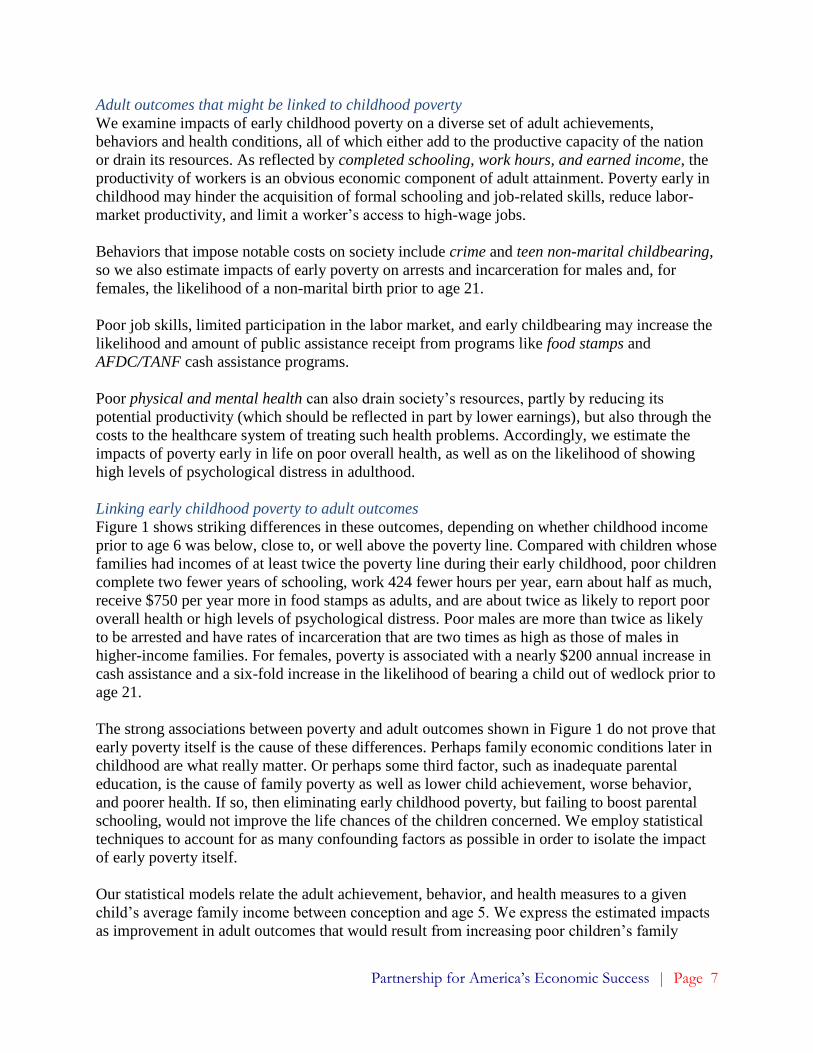


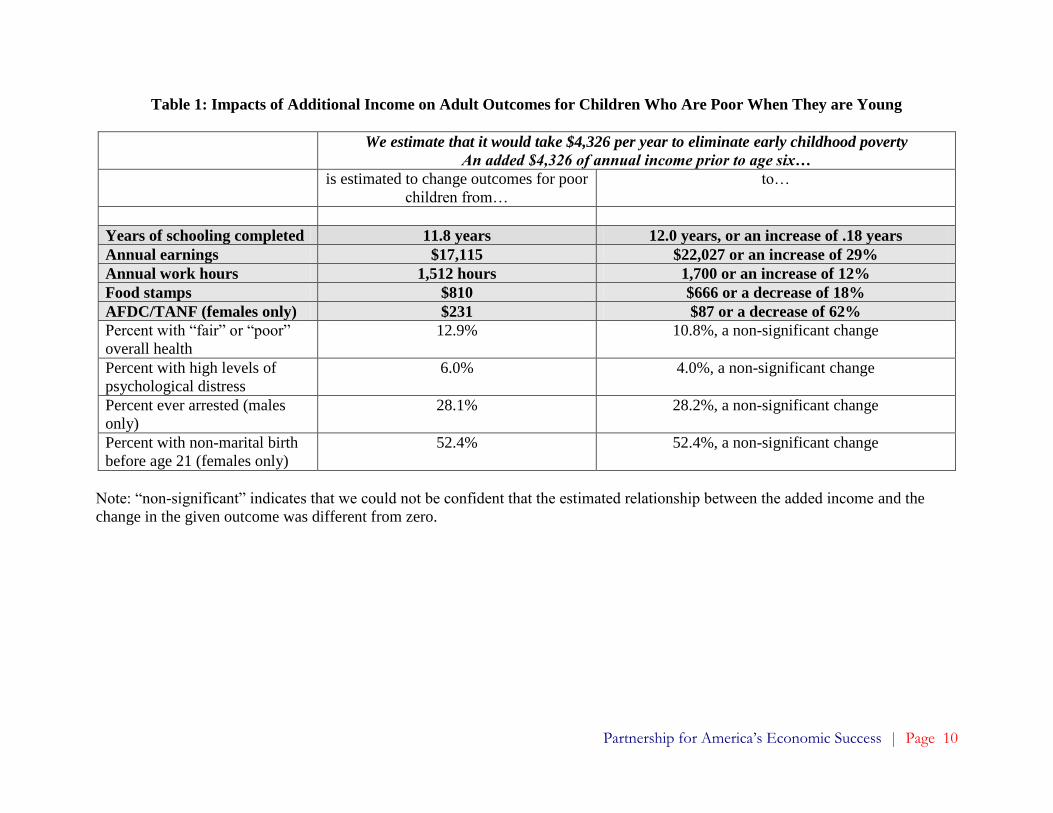


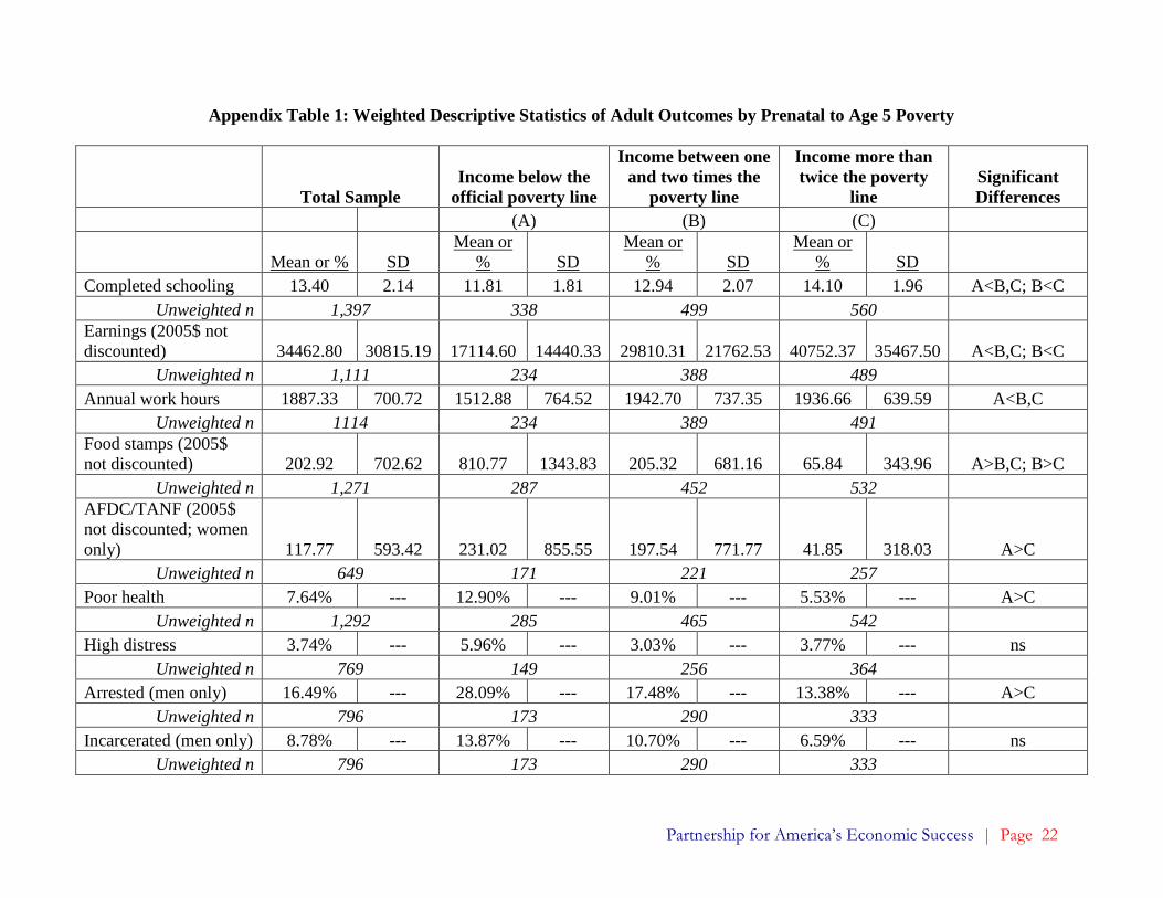


![The economic costs of childhood poverty in the United …home.uchicago.edu/ludwigj/papers/HolzerEtAlChildhoodPoverty.pdf · Downloaded By: [Duncan, Greg] At: 23:01 4 March 2008 The](https://static.documents.pub/doc/80x56/5a77ed7f7f8b9a1b688e51b9/the-economic-costs-of-childhood-poverty-in-the-united-home-downloaded-by.jpg)


