Economic Deregulation And Corporate Dividend Policy

Wayne State University

Wayne State University Dissertations

1-1-2012

Economic Deregulation And Corporate DividendPolicyXinghua GaoWayne State University,

Follow this and additional works at: http://digitalcommons.wayne.edu/oa_dissertations

This Open Access Dissertation is brought to you for free and open access by DigitalCommons@WayneState. It has been accepted for inclusion inWayne State University Dissertations by an authorized administrator of DigitalCommons@WayneState.

Recommended CitationGao, Xinghua, "Economic Deregulation And Corporate Dividend Policy" (2012). Wayne State University Dissertations. Paper 593.

http://digitalcommons.wayne.edu/?utm_source=digitalcommons.wayne.edu%2Foa_dissertations%2F593&utm_medium=PDF&utm_campaign=PDFCoverPages

http://digitalcommons.wayne.edu/?utm_source=digitalcommons.wayne.edu%2Foa_dissertations%2F593&utm_medium=PDF&utm_campaign=PDFCoverPages

http://digitalcommons.wayne.edu/oa_dissertations?utm_source=digitalcommons.wayne.edu%2Foa_dissertations%2F593&utm_medium=PDF&utm_campaign=PDFCoverPages

http://digitalcommons.wayne.edu/oa_dissertations?utm_source=digitalcommons.wayne.edu%2Foa_dissertations%2F593&utm_medium=PDF&utm_campaign=PDFCoverPages

http://digitalcommons.wayne.edu/oa_dissertations/593?utm_source=digitalcommons.wayne.edu%2Foa_dissertations%2F593&utm_medium=PDF&utm_campaign=PDFCoverPages

ECONOMIC DEREGULATION AND CORPORATE DIVIDEND POLICY

by

XINGHUA GAO

DISSERTATION

Submitted to the Graduate School

of Wayne State University,

Detroit, Michigan

in partial fulfillment of the requirements

for the degree of

DOCTOR OF PHILOSOPHY

2012

MAJOR: BUSINESS ADMINISTRATION

(Finance)

Approved by:

___________________________________

Advisor Date

___________________________________

___________________________________

___________________________________

___________________________________

ii

ACKNOWLEDGEMENTS

I would like to express my deep appreciation and gratitude to my advisor, Dr. Ranjan

D’Mello, for his patient guidance, mentorship, and support. I would not have been able to

accomplish this dissertation without his constant stimulation and inspiration. I am truly fortunate

to have had the opportunity to work with him and learn from him.

I would like to thank my committee members, Dr. Mbodja Mougoué, Dr. Margaret

Smoller, and Dr. Li Way Lee for their challenging comments and insightful suggestions which

are invaluable to the completion of this dissertation.

I would also like to thank my fellow Ph.D. students, Dr. Yonghong Jia and Dr. Mark

Gruskin for their intriguing ideas on difficult issues. Working together with them contributes to

my intellectual growth during the years of my Ph.D. study.

Thanks also go to Dr. Tim Butler, the former Ph.D. program director, for his help,

encouragement and support.

iii

TABLE OF CONTENTS

Acknowledgements ........................................................................................................................ iii

List of Tables ................................................................................................................................ viii

List of Figures ................................................................................................................................ xi

Economic Deregulation and Corporate Dividend Policy................................................................ 1

1. Introduction and Motivation ................................................................................................. 1

2. A Brief Introduction to Regulation and Deregulation in the U.S. .......................................11

3. Literature Background and Theoretical Predictions ........................................................... 15

3.1 Information content of dividend and the signaling hypothesis ........................................ 15

3.2 Agency cost theory of dividends and free cash flow hypothesis ..................................... 20

3.3 The clientele theory .......................................................................................................... 23

3.4 Dividend policy of regulated firms .................................................................................. 24

3.5 Deregulation effects on different aspect of corporations ................................................. 27

4. Hypotheses Development ................................................................................................... 29

4.1 Evolution of firms’ propensity to pay dividend in response to economic deregulation .. 29

4.2 Evolution of dividend payout in response to economic deregulation .............................. 30

4.3 Evolution of sensitivity of corporate dividend policy to earnings ................................... 32

iv

4.4 Evolution of information content of dividend policy changes ......................................... 32

4.5 Evolution of corporate financing activities in response to deregulation .......................... 34

5. The Industry Matching Method and the Three “Snapshot” Periods................................... 35

6. Data, Sample, Variable Definition, and Descriptive Statistics ........................................... 38

6.1 Data and sample construction .......................................................................................... 38

6.2 Sample distribution and dynamic changes ....................................................................... 38

6.3 Key variable definitions ................................................................................................... 41

6.4 Descriptive Statistics ........................................................................................................ 43

7. Empirical Tests ................................................................................................................... 43

7.1 Effects of deregulation on firms’ propensity to pay dividends ........................................ 44

7.1.1 Time trends in dividend payment along deregulation process .................................. 44

7.1.2 Dynamic changes of deregulated firms along deregulation process ......................... 45

7.1.3 Evolution of deregulated firms’ characteristics ......................................................... 47

7.1.4 Multivariate analysis of determinants of dividend payment ..................................... 51

7.1.5 Out of sample analysis to differentiate deregulation effects on propensity to pay.... 54

7.1.6 Which is to blame, dividend abandonment or failure to initiate?.............................. 58

7.1.7 Convergence of determinants of whether to pay between deregulated and non-

regulated firms .................................................................................................................... 60

v

7.1.8 Summary and discussion ........................................................................................... 63

7.2 Evolution of dividend payout ratio in response to deregulation ...................................... 64

7.2.1 Total deregulated firms .............................................................................................. 65

7.2.2 New entrants .............................................................................................................. 66

7.2.3 Surviving firms .......................................................................................................... 66

7.2.4 Convergence of determinants of how much to pay between deregulated and non-

regulated firms .................................................................................................................... 69


7.3 Effects of deregulation on speed of adjustment of dividend policy toward optiaml levels

................................................................................................................................................ 74

7.3.1 Lintner’s (1956) model and Fama and Babiak’s (1968) model ................................. 75

7.3.2 Regression models to test change in speed of adjustment of dividends .................... 76

7.3.3 Empirical results on change in speed of adjustment of dividends toward optimal

levels for deregulated firms ................................................................................................ 78

7.3.4 Empirical results on change in speed of adjustment of dividends toward optimal

levels for surviving deregulated firms ................................................................................ 80

7.3.5 Robustness check using three “snapshot” periods .................................................... 82


7.4 Effects of deregulation on information content of dividend policy changes ................... 83

7.4.1 Evolution of cumulative abnormal returns (CARs) around announcement of dividend

changes and dividend responsive coefficients .................................................................... 84

vi

7.4.1.1 Dividend change sample and data ....................................................................... 84

7.4.1.2 Evolution of cumulative abnormal returns (CARs) around the announcement of

dividend changes ............................................................................................................. 85

7.4.1.3 Dividend response coefficient to excess announcement returns along the

deregulation process........................................................................................................ 88

7.4.2 Evolution of relations between dividend changes and future earnings changes ....... 90

7.4.2.1 Sample and data .................................................................................................. 91

7.4.2.2 Test of relations between dividend changes and future earning changes using

linear model .................................................................................................................... 92

7.4.2.3 Test of relations between dividend changes and future earnings levels using

linear model .................................................................................................................... 93

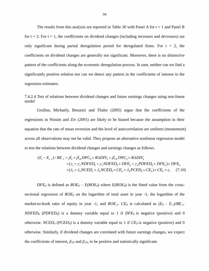
7.4.2.4 Test of relations between dividend changes and future earnings changes using

non-linear model ............................................................................................................. 94

7.4.2.5 Test of relations between dividend changes and future earnings levels using non-

linear model .................................................................................................................... 95


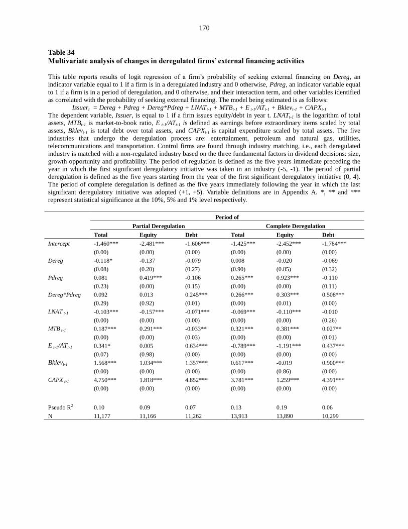
7.5 Effects of Deregulation on Corporate Financing Activities ............................................. 97

7.5.1 Evolution of frequency of external financing ............................................................ 97

7.5.2 Multivariate analysis of financing activities in response to economic deregulation . 99

7.5.3 Summary and discussion ......................................................................................... 101

8. Conclusions ...................................................................................................................... 102

vii

Appendix A. Variable Definitions ............................................................................................... 104

Appendix B. Figures ................................................................................................................... 104

Appendix C. Tables ..................................................................................................................... 104

References ................................................................................................................................... 171

Abstract ....................................................................................................................................... 185

Autobiographical Statement…….………………………………………………………………187

viii

LIST OF TABLES

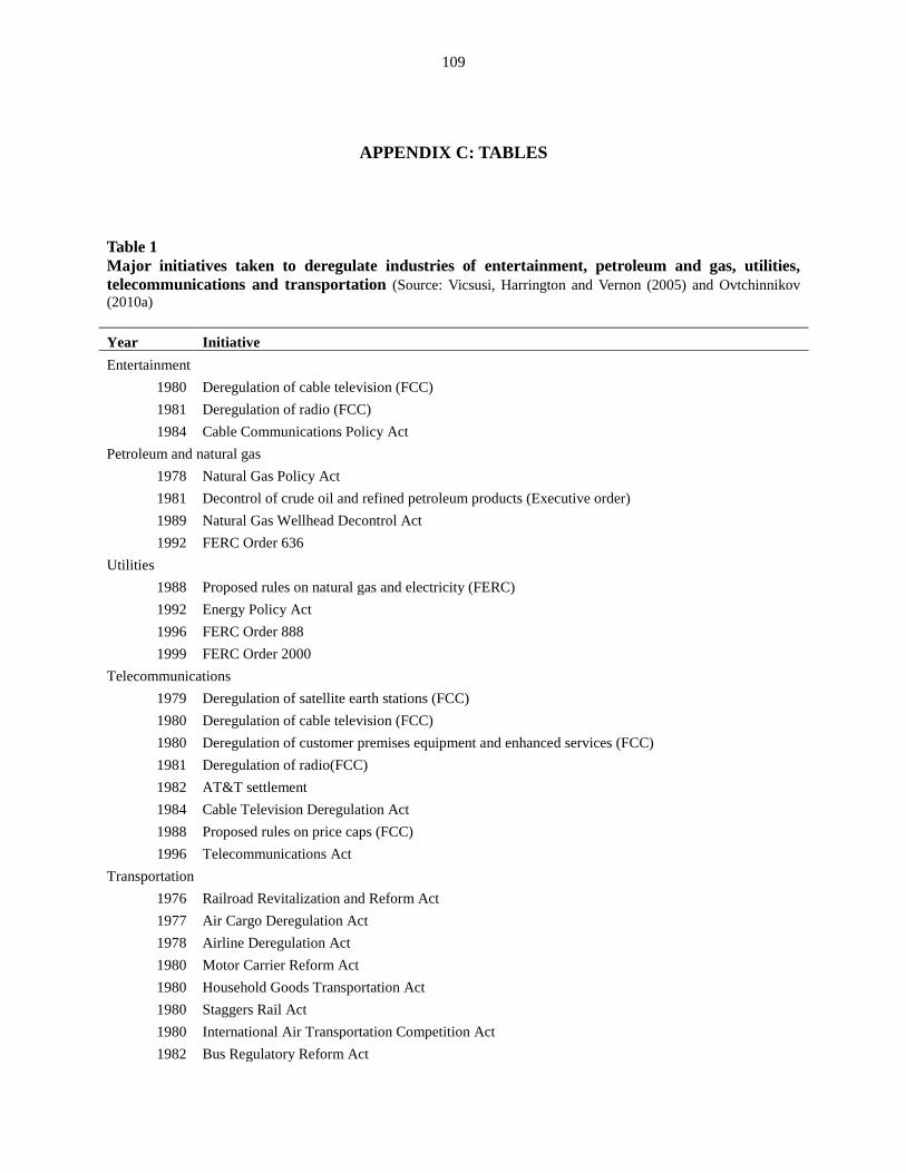
Table 1: Major initiatives taken to deregulate industries of entertainment, petroleum and natural

gas, utilities, telecommunications and transportation ……………………….……..…108

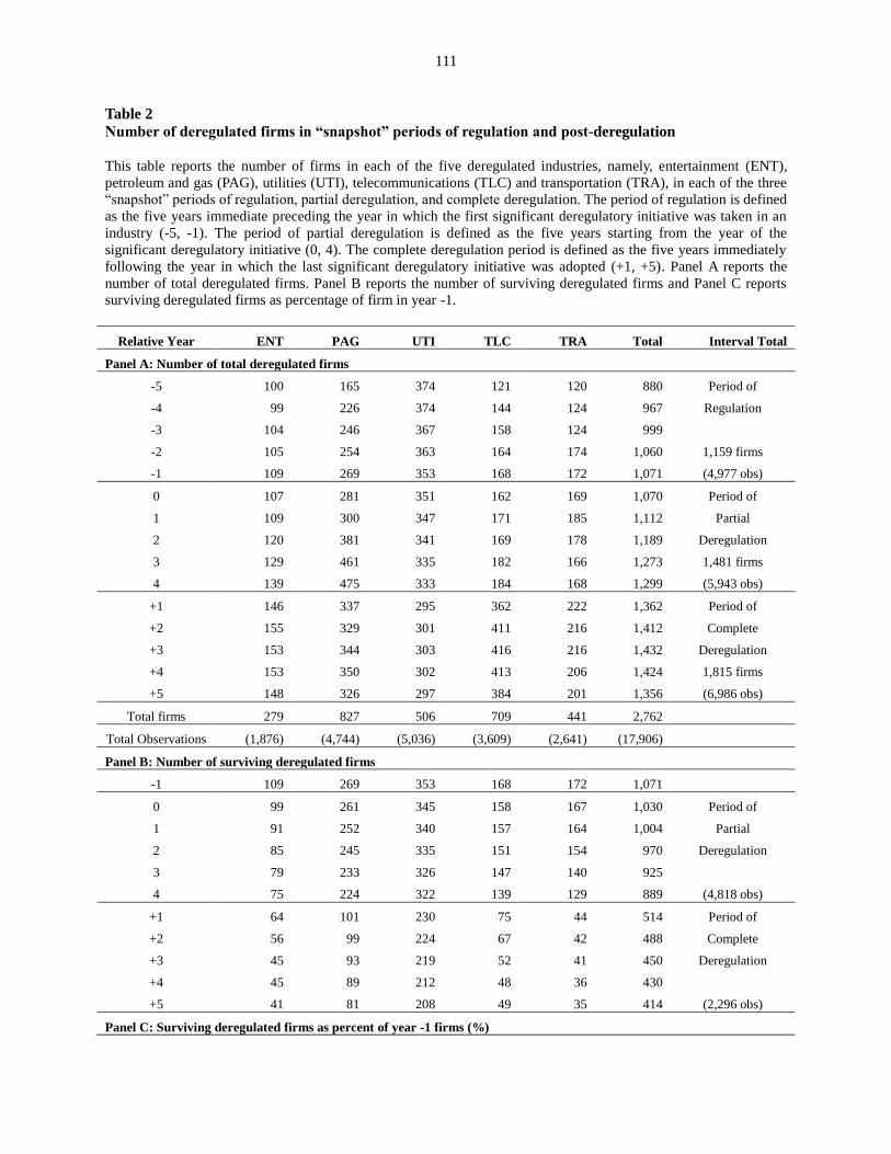
Table 2: Number of deregulated firms in “snapshot” periods of regulation and post-deregulation

.................................…………………………………………………………………..….……..109

Table 3: Number of new entrants, exits and existing firms in year t relative to year -1 in

deregulated industries…………………………………………………………..……...111

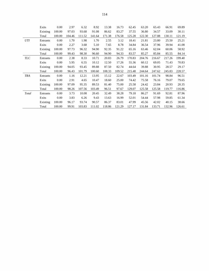
Table 4: Number and percentage of new entrants, exits and existing firms in post-deregulation

“snapshot” periods relative to year -1 for deregulated industries……………...….…...113

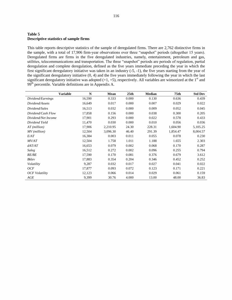
Table 5: Descriptive statistics of sample firms………………………………………………....114

Table 6: Dynamic changes of dividend payers and non-payers in year -1 over the process of

deregulation……………..…………………………………………………………..…115

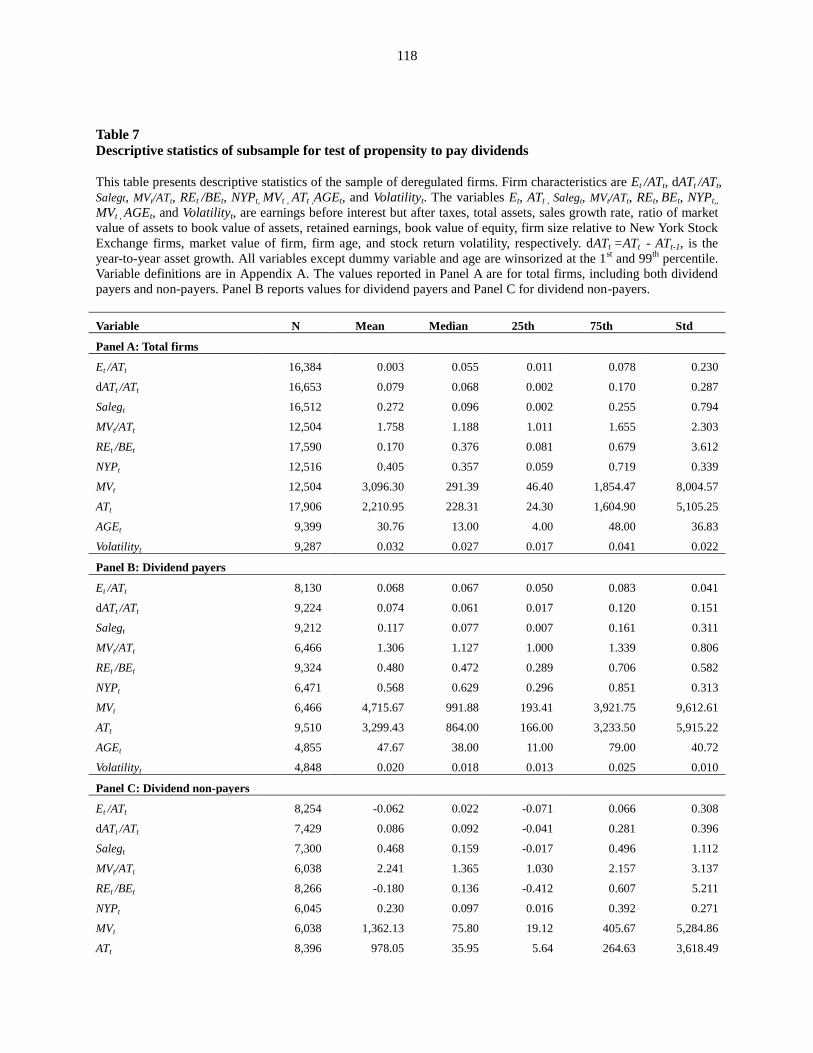
Table 7: Descriptive statistics of subsample for test of propensity to pay dividends………..…116

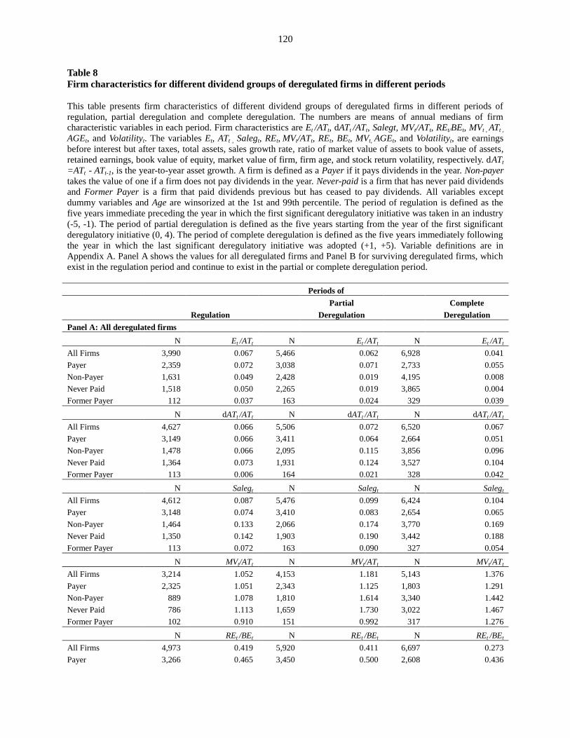
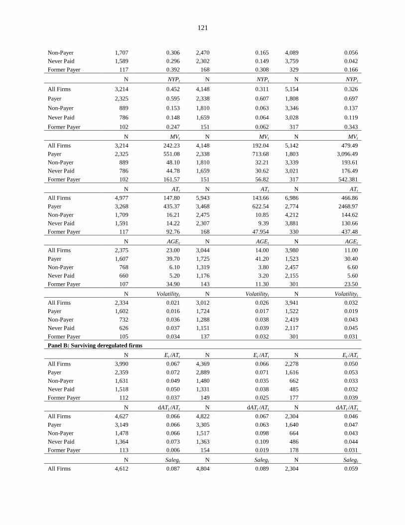
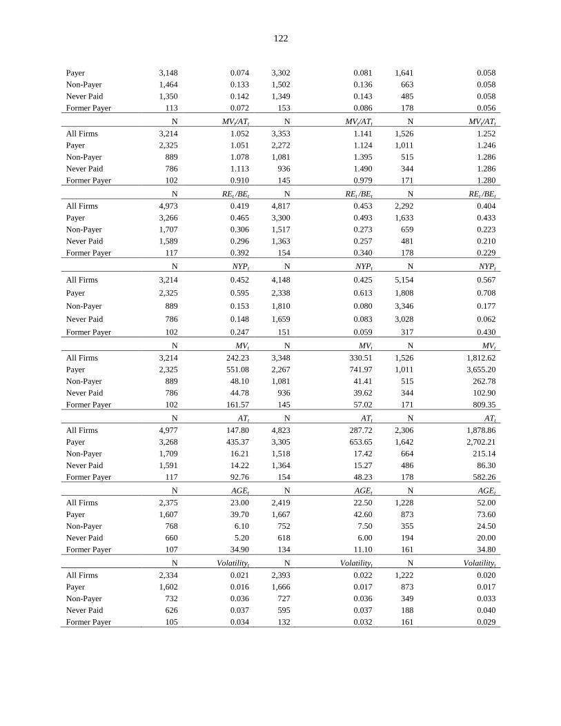
Table 8: Firm characteristics for different dividend groups of deregulated firms in different

periods……………………………………………………………………….…..….....118

Table 9: Logit regressions to explain deregulated firm decision to pay or to not pay dividends in

three periods…………………………………………………………………..…..…...121

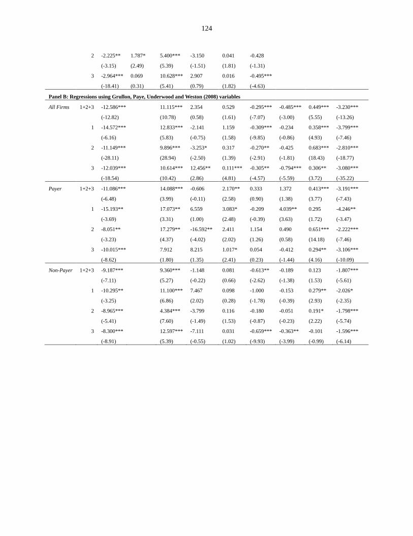
Table 10: Out of sample estimates from logit regressions of the effect of changing firm

characteristics and deregulation on percent of firms paying dividends……...…..….123


characteristics and deregulation on percent of firms paying dividends using all

Compustat firms as controls………………..………………………………..……...125


characteristics and deregulation on percent of firms paying dividends using eight

randomly selected industries as controls………………….…………………...….…127

Table 13: Dividend abandonment versus failure to initiate………………………………….…129

Table 14: Convergence of determinants of propensity to pay dividends for partial and complete

deregulation periods…………………….…………..………………….……………130

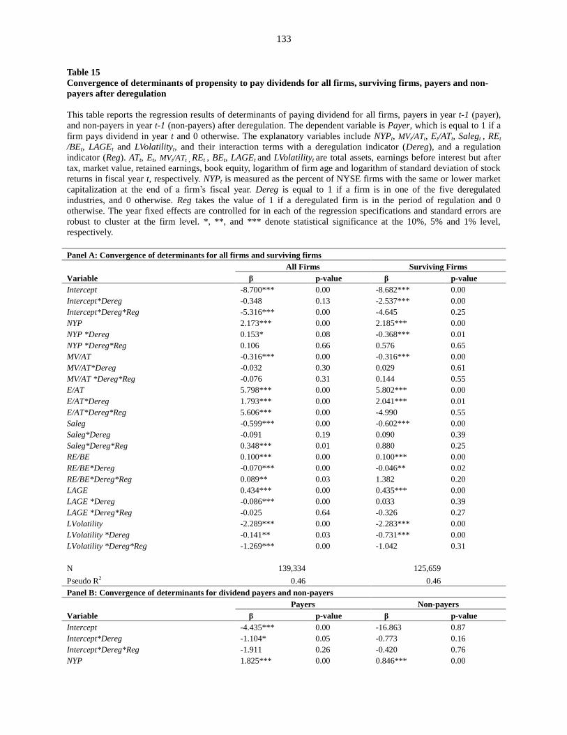
Table 15: Convergence of determinants of propensity to pay dividends for all firms, surviving

ix

firms, payers and non-payers post deregulation……….……...……………….….…131

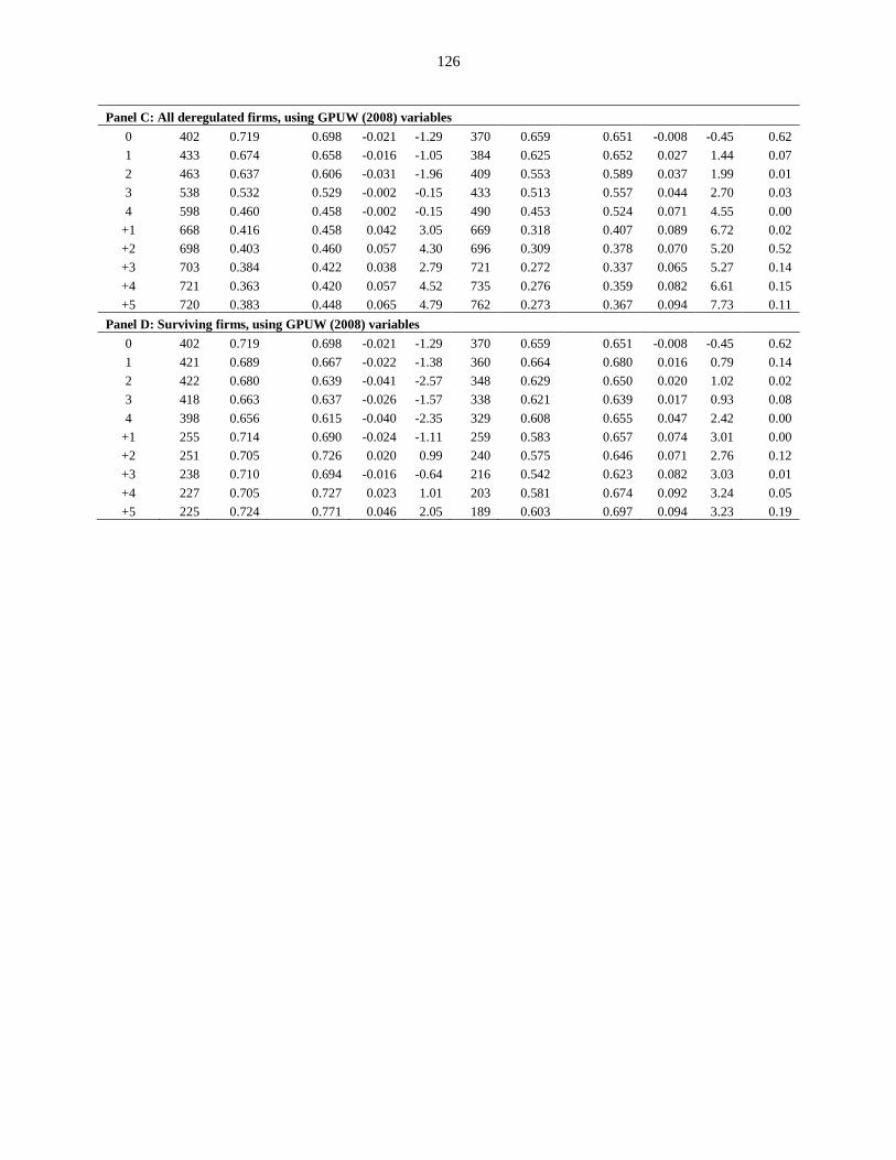
Table 16: Estimation of effect of regulatory changes on firm dividend payout in “snapshot”

periods…………………………….………………………….………….…….…….133

Table 17: Difference-in-differences estimation of effect of regulatory changes on firm dividend

payout in “snapshot” periods………………………….…….………….……….…..134

Table 18: Robustness check of difference-in-differences estimation of effect of regulatory

changes on firm dividend payout……………….………………….………….…….135

Table 19: Difference-in-differences estimation of effect of regulatory changes on firm dividend

payout, 1966-2008……………………………..………….……………….……...…136

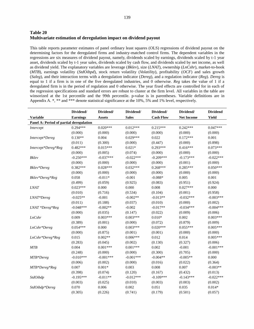
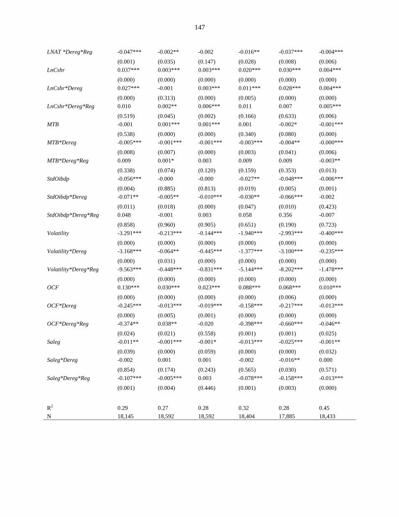
Table 20: Multivariate estimation of deregulation impact on dividend payout……..….………137

Table 21: Robustness check on multivariate estimation of deregulation impact on dividend

payout: excluding observations with negative earnings, net income or cash flow.….143

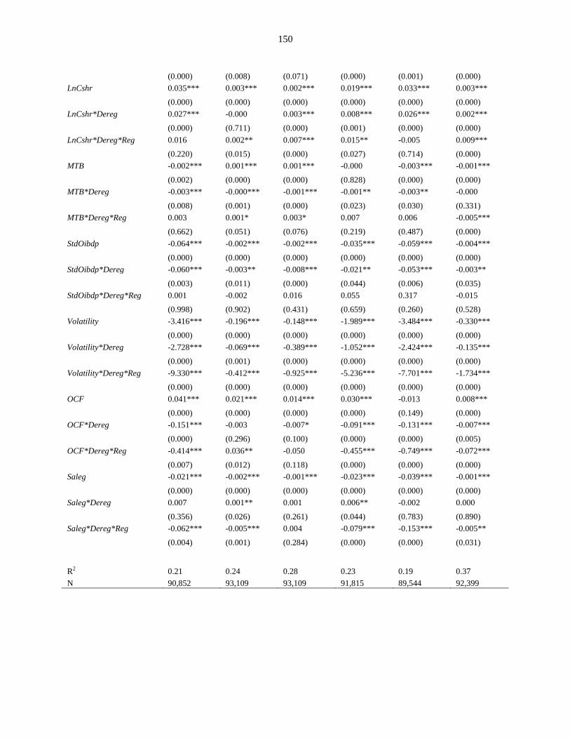
Table 22: Robustness check on multivariate estimation of deregulation impact on dividend

payout: using all Compustat firms from 1966 to 2008…………...……….……....…146

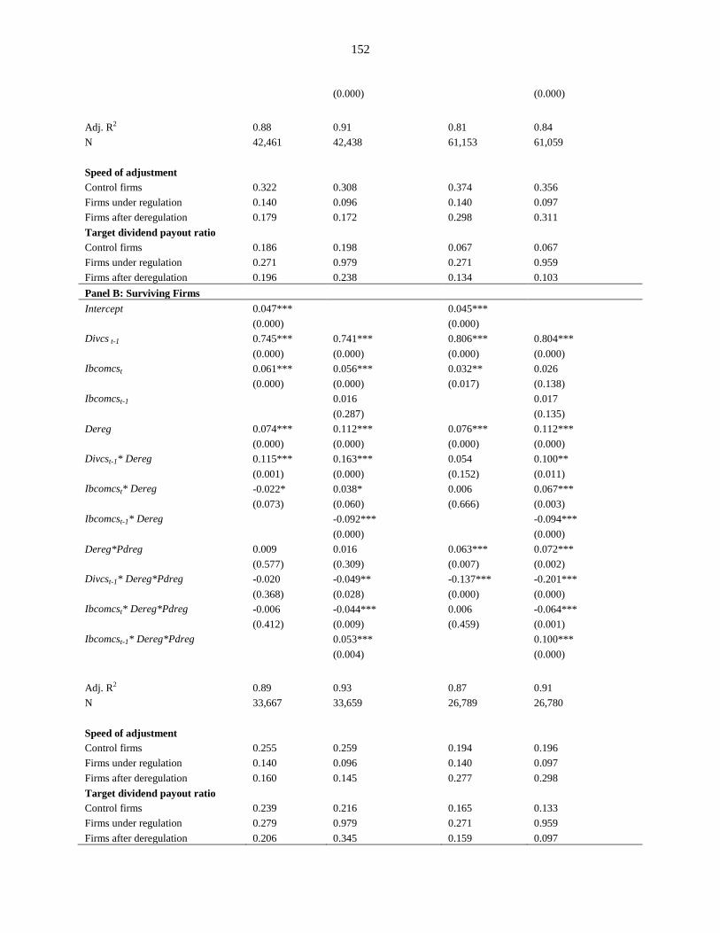
Table 23: Regression-based evidence based on Lintner and Fama-Babiak models of partial

adjustment of dividend policy, 1966-2008………………….….…………….….…..149

Table 24: Regression-based evidence based Lintner and Fama-Babiak models of partial

adjustment of dividend policy in “snapshot” periods……………….…..…….……..151

Table 25: Magnitude of dividend increases and decreases during the process of deregulation

…………………………………………………………………………………………..……....153

Table 26: Dividend announcement CARs during different periods of the deregulation process

…………………………………………………………………………………………….…….154

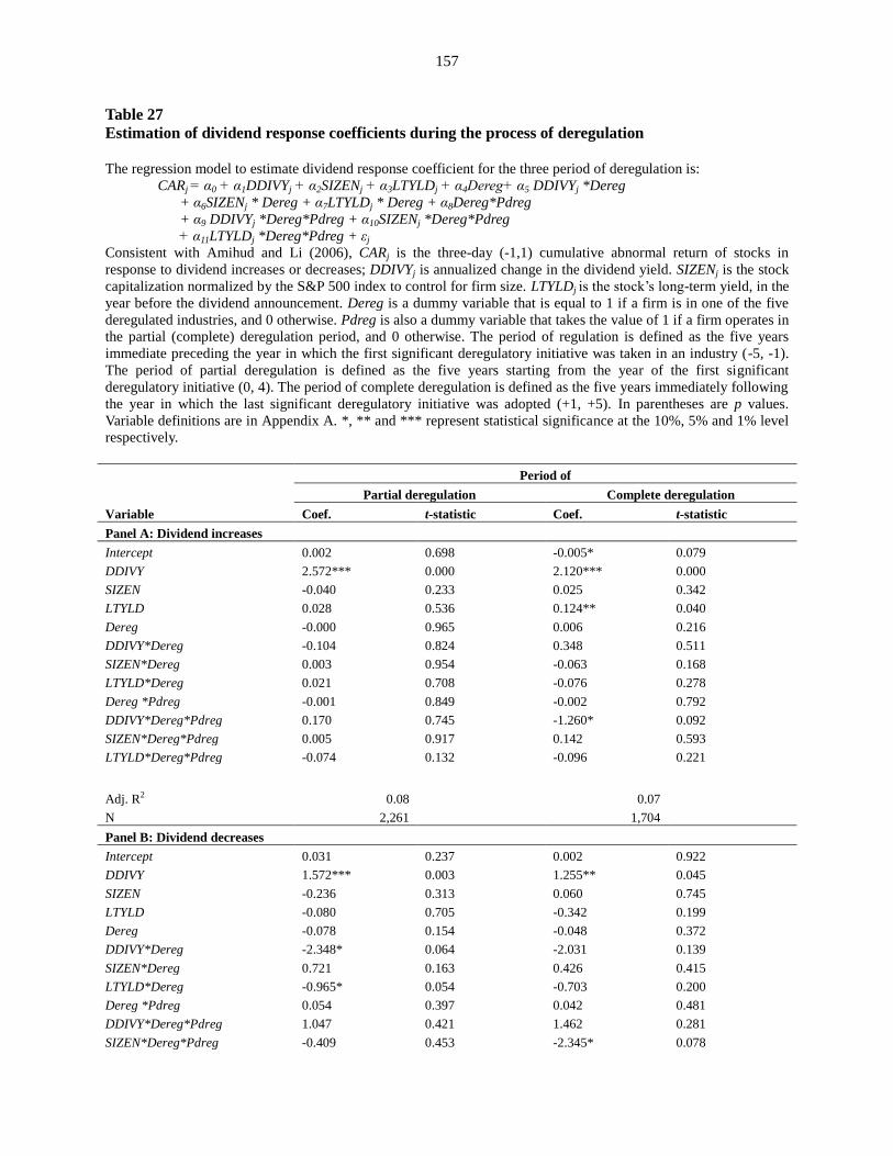
Table 27: Estimation of dividend response coefficients during the process of deregulation

…………………………………………………………………………………………….….....155

Table 28: Summary statistics of the subsample of firms that increase, decrease or maintain

dividends…………………..…………….……………………………………….….157

Table 29: Regressions of future earnings changes on dividend changes using linear model

…………………………………………………………………………………………..…..…..158

Table 30: Regressions of future earnings levels on dividend changes using linear model

………………………………………………………………………………………….………160

x

Table 31: Regressions of future earnings change on dividend changes using nonlinear model

……..…………………………………………………………………………………………...162

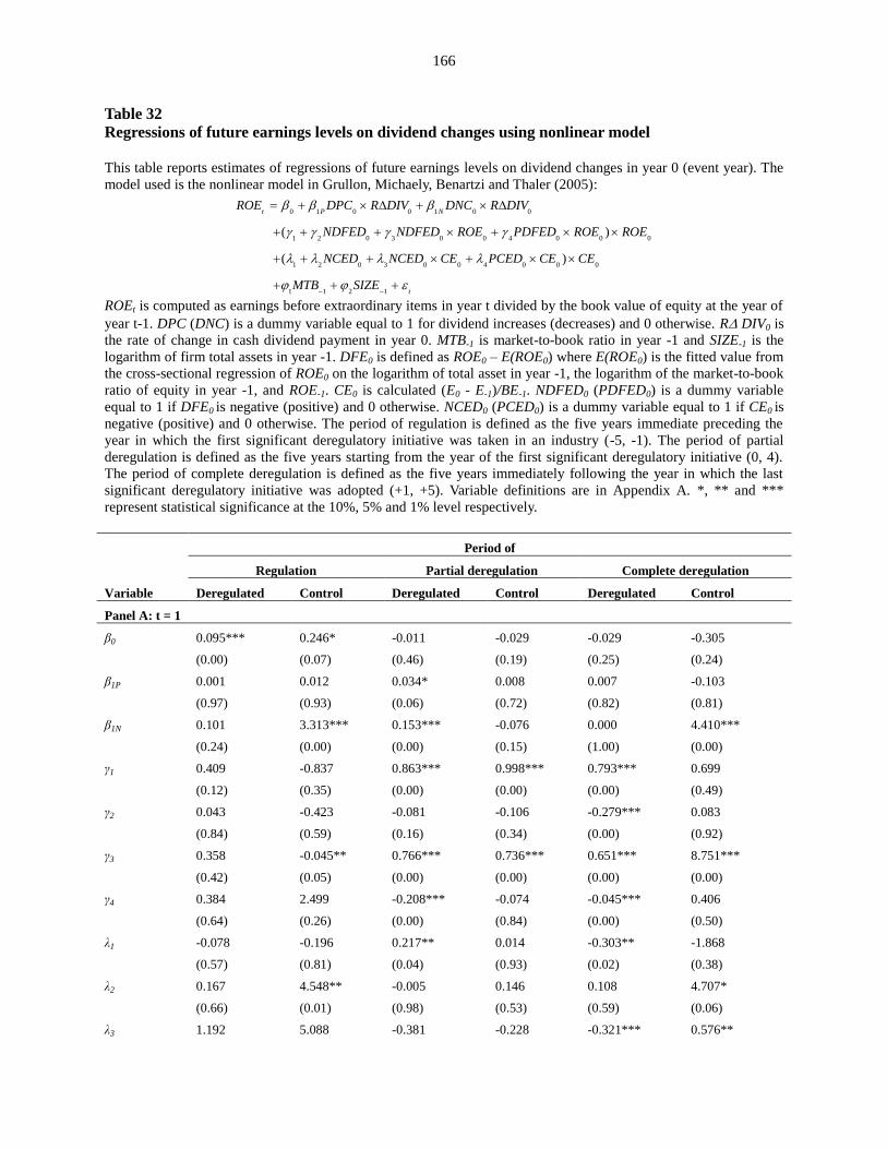
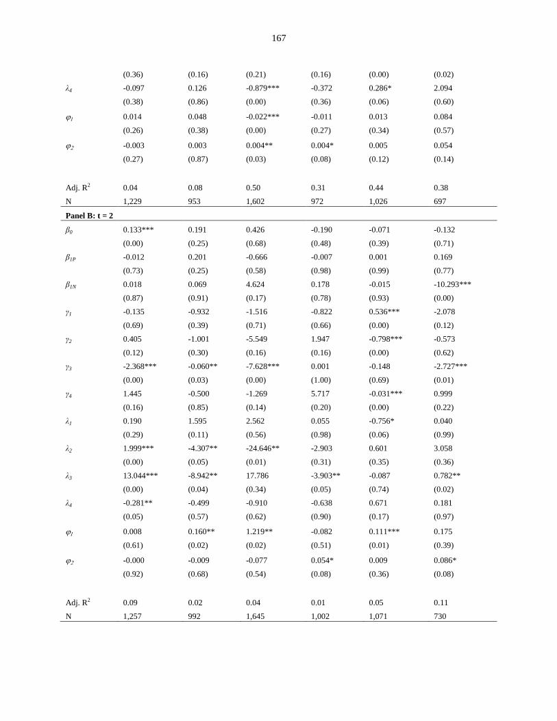
Table 32: Regressions of future earnings levels on dividend changes using nonlinear model

……...……………………………………………………………………………………..…….164

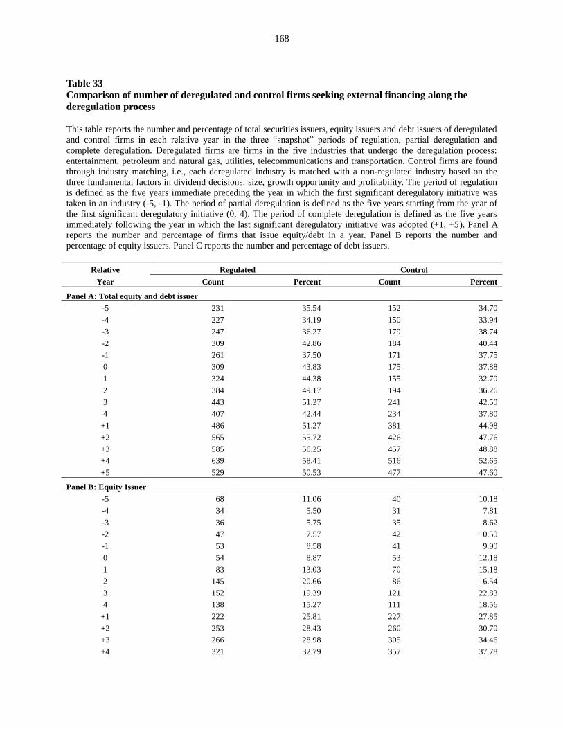
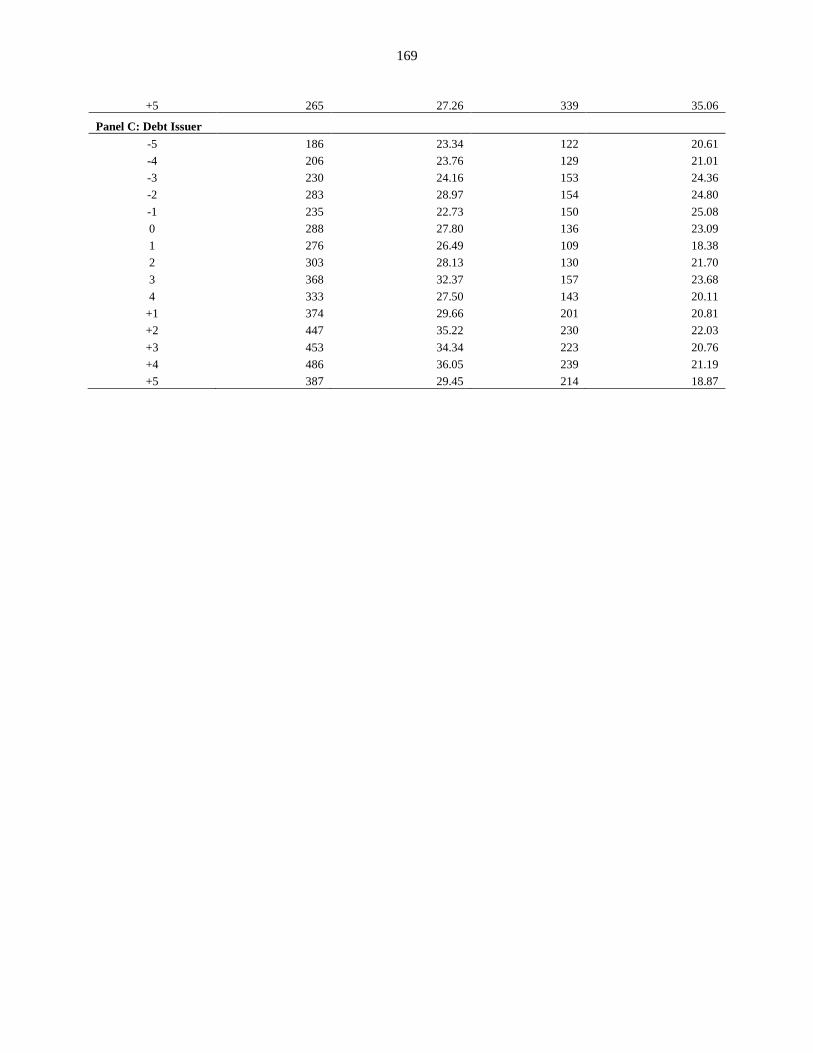
Table 33: Comparison of number of deregulated and control firms seeking external financing

along the deregulation process…………………..…….…………………………….166

Table 34: Multivariate analysis of changes in deregulated firms’ external financing activities

………..………………………………………………………………………….…………..…168

xi

LIST OF FIGURES

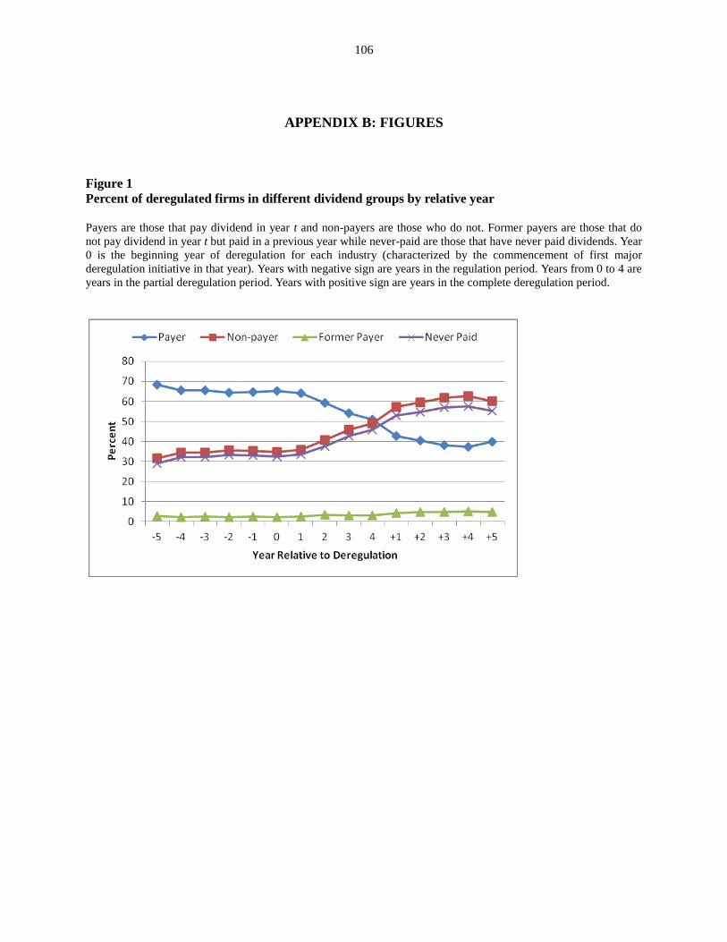
Figure 1: Percent of deregulated firms in different dividend groups by relative year………….105

Figure 2: Dividend payouts of all deregulated firms and control firms…………….…………..106

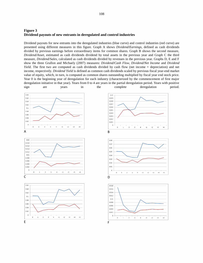
Figure 3: Dividend payouts of new entrants in deregulated and control industries………...…..107

.

1


1. Introduction and Motivation

Why did firms pay dividends even though dividends were subject to higher taxation than

other means of income distribution? This question has been puzzling financial economist for

decades. Miller and Modigliani (1961) propose a theory of irrelevance based on the perfect

financial world assumptions, in which a firm’s value is not affected by its dividend policy.

Although a relaxation of the assumptions leads to predictions otherwise, the seminal work of

Miller and Modigliani (1961) has inspired a growing academic interest in exploring firms’

dividend policy. Voluminous studies have attempted to answer the fundamental question – “why

do firms pay dividends” and its accompanying question – “how do firms formulate their dividend

policy.”

Generally speaking, three theories have been developed around the questions concerning

corporate dividends. The information content theory posits that dividends reveal a firm’s

proprietary information that is unable to be disclosed directly through other means and that

dividends also reflect managers’ forecast of corporate earnings prospects (see, e.g., Bhattacharya

(1979); Miller and Modigliani (1961); Miller and Rock (1985)). Its variant signaling hypothesis

further suggests that firms use dividends to signal their quality in order to differentiate

themselves from lower quality firms (see, e.g., Healy and Palepu (1988); Lang and Litzenberger

(1989)). The agency theory argues that firms distribute cash flows in the form of dividend to

shareholders to minimize agency costs to the extent that hoarding cash tacitly encourages

managers to overinvest (in projects with negative net present value), facilitates their perquisite

2

consumption, and insulates them from capital market monitoring and discipline (Jensen and

Meckling (1976); Jensen (1986); and Easterbrook (1984)). This function of dividends is all the

more important when the market for corporate control is severely constrained by regulations in

the regulated industries, and dividends thus serve as an alternative to the threat of takeover as a

way of reducing agency costs.1 The tax-based clientele theory suggests that firms pay out

dividends to attract target investor constituencies in different tax brackets. For example, high

dividends are used to attract informed institutional investors that are tax-advantaged and can

furnish more effective monitoring (see, e.g., Allen, Bernardo and Welch (2000); Redding (1997);

Shleifer and Vishny (1986)), and firms may initiate or omit dividends to cater to changing

demands of investors (Baker and Wurgler (2004)).

There are two major theories concerning how firms formulate their dividend policy,

which have their antecedents in the capital structure literature: the trade-off theory and the

pecking order theory. The trade-off theory (see, for example, Fama and French (2002); Kraus and

Litzenberger (1973); Myers (1984)) suggests that firms balance the costs and benefits of paying

dividends to derive an optimal dividend policy. Specifically, they consider the benefits of

reduced agency costs associated with dividend payout and the costs of possible future cash

shortage and potential increased conflicts between equity and debt holders. The pecking order

theory suggests that firms prefer internal financing to safe debt, safe debt to risky debt, and

finally risky debt to equity financing. As such, given profitability, firms like to retain a greater

portion of operating income rather than dispense it through dividend payment to shareholders.

This theory implies that there is no optimum dividend payout.

Despite intensive research and theoretical development, empirical evidence from testing

1 It is documented in the literature that corporate takeover activities are significantly restricted in regulated industries,

the utilities industry in particular. For details, see, e.g., McLaughlin and Mehran (1995) and Cox and Portes (1998).

3

predictions of some of these theories appears to be weak or sometimes contradictory. For

example, empirical tests indicate that dividend changes are at best poor predictors of future

earnings levels or earnings changes (see, for example, Benartzi, Michaely and Thaler (1997);

Grullon, Michaely, Benartzi and Thaler (2005)). Also, although empirical evidence is largely

consistent with agency explanations that dividends dissipate firms’ discretionary cash flows to

help reduce agency costs, questions arise as to why the more tax-advantageous share repurchase

should not be used completely in lieu of dividend payment, given that repurchase achieves the

same goal of disgorging cash without committing the firm to regular cash outlays. As for the

clientele theory, contradictory evidence is provided by, among others, Grinstein and Michaely

(2005), which shows that although institutions choose to stay away from firms that do not pay

dividends, they in fact prefer those firms that pay fewer dividends, which is somewhat

inconsistent with the tax-based clientele hypothesis. Further, while Michaely, Thaler and

Womack (1995) fail to detect any significant institutional clientele migration following dividend

omissions, Brav and Heaton (1998) do find pension funds reduce their holdings of dividend-

omitting stocks in conformity with the strict “prudent man” rule after the enactment of the

Employee Retirement Income Security Act of 1974 (ERISA). Interestingly, Hoberg and Prabhala

(2009) challenge the “catering” theory of Baker and Wurgler (2004) by contending that the

relation between transient investor fads of dividends and dividend changes disappears after

controlling for the risk factor.

Yet making the dividend issue even more puzzling and complicated is the evidence

presented by Fama and French (2001). They report strikingly disappearing dividends – that is,

during the two decades between 1978 and 1999, cash dividend-paying firms drop from 66.5

percent to 20.8 percent. There is some evidence that this declining propensity to pay dividends

4

also occurs outside the U.S., although the evidence is not as compelling as in the U.S. (Denis and

Osobov (2008)).2 As such, it appears that dividends have remained largely the same puzzle as

described in Black (1976).3 The mixed evidence has left the most fundamental question of why

firms pay dividends largely unanswered.

Economic deregulation, which swept the U.S. from the 1970s to the 1990s, offers a

unique setting to study the dividend issue. The deregulation process, hailed as “one of the most

important experiments in economic policy of our time” (Winston (1993)), is characterized by

governments’ withdrawal from active role in governing business decision-making and activities

such as pricing, output, entry and exit (Hahn (1990); Winston (1993)). Deregulation opens the

door to a competitive operating environment, which is fundamentally different from the one pre-

deregulation. The deregulation course has significant effects on the U.S. economy.4 More

importantly, as a major economic shock to firms’ operating environments, economic deregulation

provides a “natural experiment” to empirically test various predictions of financial theories.5 For

example, previous research documents that the deregulation process has significantly affected

deregulated firms’ corporate governance mechanisms (Kole and Lehn (1997)), capital structure

2 Denis and Osobov (2008) extends the study of declining propensity to pay to such developed financial markets as

Canada, the United Kingdom, Germany, France and Japan and finds similar trend in those countries. Interestingly,

the factors that explain the drop in dividend payment in the U.S. market maintain their explanatory power beyond

the U.S. borders. 3 Black (1976) first used the term “the dividend puzzle” to describe the perplexing nature of firms’ dividend payment

in his article with this term as its title. “The harder I look at the dividend picture, the more it seems like a puzzle

with pieces that just don’t fit together,” he writes in the essay. Numerous researchers have since tried to find answers

to the puzzle; however, the main questions relevant to the puzzle remain unresolved. 4 A little more than three decades ago, regulated industries produced approximately 17 percent of U.S. economic

output; by 2007, however, those industries – entertainment, transportation, telecommunications, petroleum and

natural gas, utilities, and financial services, whose large parts are completely deregulated – made up roughly 7

percent of the U.S. gross national product. This figure was first provided by Winston (1993) and used extensively by

deregulation researchers subsequently, e.g., Kwoka (2002). For details, see U.S. Bureau of Economic Analysis

releases. http://www.bea.gov/. 5 Deregulation is mainly regarded by researchers as an exogenous shock. See, e.g., Kole and Lehn (1999). However,

extant theories about the exogeneity of deregulation is argued against by Ovtchinnikov (2010b), which suggests that

deregulation reform was in response to worsening industry conditions and pressures from special interest groups,

thus “not unexpected and exogenous.”

http://www.bea.gov/

5

choices (Ovtchinnikov (2010a)), and investment policies (Ovtchinnikov (2010b)).

In the same vein, economic deregulation should impact firms’ dividend policy as well.

Since the new competitive environment in which firms are operating is vastly different from the

environment when regulations are in place, deregulation touches upon every aspect of the

business world, providing a more level playing field and introduces new rules for the game. For

example, deregulation tends to increase information asymmetries between insiders and outsiders

(e.g., Barclay and Smith (1995); Krishnaswami, Spindt and Subramaniam (1999); Ovtchinnikov

(2010a)), reduce agency costs associated with shareholder-regulator conflicts (e.g., Easterbrook

(1984); Smith (1986)), and change the composition of clientele (e.g., Baker and Wurgler (2004);

Shleifer and Vishny (1986)). These are among the elements believed to be closely associated

with firms’ dividend policy. As such, the theories regarding information content, agency-

principle conflict and shareholder clientele have theoretical predictions with regards to corporate

dividend policy for firms whose industry undergoes the deregulation process.

Conspicuously absent from this literature, nevertheless, is whether and to what extent

economic deregulation impacts firms’ dividend policy. This study aims to fill this gap by

examining the evolution of dividend policy in response to the changing operating environment

along the economic deregulation process. Specifically, I examine the effects of deregulation on

firms’ propensity to pay dividends, how deregulation affects the level of dividends paid, whether

deregulation makes firms’ dividend policy more sensitive to operating income, and how

information content of dividend changes in response to deregulation. The new perspective I

attempt in this research will shed some insights that can be conducive to a better understanding

of the complex “dividend puzzle” and contribute to the effort of demystifying the puzzle.

I begin by investigating whether deregulation impacts firms’ propensity to pay dividends.

6

Smith (1986) argues that firms under regulation pay high dividends to control agency problems

between shareholders and managers as well as between shareholders and regulators. Distributing

cash in the form of dividend not only reduces cash flows available for spending at the discretion

of managers but also creates demands for external financing that helps keep regulated firms in

the financial market, which provides monitoring and serves as a reminder of the current cost of

capital to regulators and stakeholders alike. Deregulation eventually helps remove the agency

problem between shareholders and regulators (regulators are gone, probably forever, for these

industries), and the deregulated firms and their non-regulated counterparts are faced with similar

situations of agency problems. Therefore, from an agency perspective, I predict a decline in firms’

inclination to pay dividends following deregulation. Deregulation also abolishes restrictions on

investment so that deregulated firms are faced with an expanded investment opportunity set (see,

e.g., Barclay and Smith (1995); Smith and Watts (1992)).6 In addition, deregulation-induced

competition increases operating and earnings uncertainty, raising the possibility of financial

distress. Accordingly, the operating environment changes are expected to reduce firms’

predilection to pay dividends. On the other hand, the signaling theory suggests that the

competitive environment induced by economic deregulation may incentivize quality firms to

signal their strength in the face of growing competition, thus making those high performers more

willing to pay dividends. Ultimately, the propensity to pay dividends of deregulated firms along

the deregulation process is an empirical question.

Next, I examine whether economic deregulation affects the level of dividends paid. The

distinctive double agency problems between shareholders and management, and between

6 Smith and Watts (1992) contend that regulation restricts a firm’s investment opportunity set and “makes

observation of the manager’s actions easier.” Empirical evidence is supplied by Barclay and Smith (1995), who find

that regulated firms, like large firms, have more long-term debt, consistent with the argument that firms with more

investment opportunities have less long-term debt in their capital structure.

7

shareholders and regulators, encountered by firms in the regulated industries also imply that

those firms have higher dividend payout ratio, e.g., paying out the bulk of cash flows to reduce

agency costs and create opportunities for market monitoring and discipline. The elimination of

agency conflicts between regulators and shareholders makes it less necessary for deregulated

firms to maintain high dividend payouts. Similarly, changes in the operating environment, such

as expanded investment opportunities, heightened competition, and increased level of cash flow

volatility, make internally generated funds more valuable to financing future investment

opportunities and hedge against potential cash flow shortfalls. All these, therefore, lead to a

prediction of lower dividend payout by deregulated firms along the process of economic

deregulation. On the other hand, the clientele theory suggests that in an effort to maintain their

tax-based clienteles, firms would avoid drastic dividend policy changes despite fluctuations in

earnings and in times of earnings uncertainty (Graham and Kumar (2006); Lewellen, Stanley,

Lease and Schlarbaum (1978)). Conversely, changes in the composition of clientele may lead to

firms’ amending their dividend policy to accommodate new needs (e.g., Becker, Ivković and

Weisbenner (2011)). Kole and Lehn (1999) report a concentration of equity ownership by outside

block-holders after deregulation. This shift toward higher block-holdings may not give rise to

higher dividend payouts since institutional investors favor fewer dividends to more dividends

(Grinstein and Michaely (2005); Jain (1999); Strickland (2002)). Meanwhile, the signaling

theory predicts that high quality firms would more likely use dividends as a signal to distinguish

them from lower quality firms in a competitive environment. Therefore, the impact of the

economic deregulation on dividend payout ratio is also an empirical issue.

I proceed to investigate whether firms’ dividends are adjusted at greater speed toward

target dividend payout ratio in response to deregulation. Lintner (1956) suggests that firms set

8

target dividend payouts and would adjust their dividends toward the targets based on firms’

earnings conditions. Firms under regulation are protected from market competition, and

dividends may be a less important component of firms’ effort to adjust to the overall risk they are

faced with. However, deregulation positions deregulated firms on the same playing field as non-

regulated firms and may require firms to react faster to elevated competition and heightened

uncertainty. Accordingly, I predict that firms’ dividend policy will become more sensitive to

changes in earnings and the adjustment toward target dividend payout will occur more quickly, in

response to changes in the operating environment induced by economic deregulation.

I then study whether the deregulation process changes the information content of

dividends. Economic deregulation is expected to make firm operations less transparent and

increase the information asymmetry between insiders and outsiders (Krishnaswami, Spindt and

Subramaniam (1999); Ovtchinnikov (2010a)).7 The theories of information content and signaling

argue that the dividend signaling becomes more important in situations of high information

asymmetry, thus eliciting greater stock price reactions to financing announcements in this

scenario (Smith (1986)). I thus explore the impact of economic deregulation on the information

content of dividends by investigating changes in the stock market valuation reaction to

announcements of dividend changes along the economic deregulation process and the relation

between dividend changes and future earning and changes in earnings.

Lastly, I examine changes in firms’ external financing activities during the post-

deregulation periods. On the one hand, the argument that regulated firms pay high dividends to

dissipate free cash flow to control the double agency problems and to procure capital market 7 Krishnaswami, Spindt and Subramaniam (1999) examine the proportion of privately placed debt in firm debt

structure and find that firms with favorable information about their earnings prospects but subject to great

information asymmetry use more private debt. Regulated firms, however, are found to have lower proportions of

privately placed debt. Ovtchinnikov (2010a) notes two likely reasons for higher degree of information asymmetry

after deregulation: the removal of regulatory monitoring and the firm inclination to keep proprietary information

from rivals and the general public in more competitive environments.

9

monitoring and discipline indicates high frequency of external financing activities of firms under

regulation. On the other hand, enhanced competition and expanded growth opportunities in the

wake of economic deregulation may increase firms’ needs for external capitals, leading to more

active external financing activities. Thus, how deregulation impacts firms’ external financing

behavior is an empirical issue.

My empirical results reveal that economic deregulation does not have significant

incremental impact on firms’ decisions regarding whether to pay dividends after controlling for

the effect of changing firm characteristics and the general trend of declining propensity to pay

dividends. However, there is evidence that economic deregulation affects dividend payers’

decisions on how much to pay. Using the difference-in-differences approach to control for the

effects of time trend, I find that not only firms in the deregulated industries, but also those

surviving deregulated firms, lower their dividend payout ratio along the deregulation process.

More importantly, empirical evidence shows an upward trend in the speed of adjustment of

corporate dividend policy to optimal levels and a declining trend in firms’ target payout ratio,

indicating that deregulated firms respond to the changing operating environment brought about

by economic deregulation by connecting their dividend policies more closely with earnings.

In an attempt to examine whether the changing operating environment brought on by the

economic deregulation affects the information content of dividend, I investigate the evolution of

cumulative abnormal returns (CARs) around the announcement of dividend changes and the

association of dividend changes with future earnings and profitability. The empirical results

provide little evidence of an upward trend in CARs or an association between dividend changes

and future earnings, rendering little support to the prediction that firms are more likely to signal

information using dividends in the post-deregulation periods. In analyzing the changing external

10

financing activities, I find that deregulated firms increase external financing activities steadily

immediately after the deregulation initiatives and accelerate equity and debt issuance as the

deregulation process progresses. This pattern mirrors the evidence I document earlier regarding

the magnitude of dividend payouts: the further into the deregulation process, the greater the

impact of deregulation on corporate dividend policy. The overall evidence indicates that changes

in dividend policy along the deregulation process are partly a result of enhanced market

monitoring and discipline arising from the more frequent external financing activities of

deregulated firms.

The study is related to two lines of literature. The first is the literature on economic

deregulation. Economic deregulation puts an end to the government role in controlling price,

rates of return, entries or exits, and production, and heralds in an environment of competition

which leads to changes in firms’ investment opportunity set, earnings volatility, profitability,

financing costs and bankruptcy costs, etc. Prior research has documented that firms react to the

changing environment by adjusting their financing policy and capital structure (Ovtchinnikov

(2010a)) and governance structure (Kole and Lehn (1999)). I complement this line of research by

investigating the impact of the economic deregulation on firms’ dividend policy. Unlike changes

in firm capital structure that occur almost in immediate response to economic deregulation,

adjustments in corporate dividend policy are shown to be gradual, which not only is consistent

with the notion that dividends are sticky, but also reflects the complexity in formulating checks

and balances in mitigating the agency problem. The overall results indicate that economic

deregulation has some bearings on corporate dividend policy, as well as on different aspects of

corporate financing, investment and operation decisions.

Second, the study adds to the literature on dividend policy and its determinants. As

11

mentioned earlier, there is a rich body of research on dividend policy; however, the empirical

evidence has been mixed and some of the research designs and methodologies suffer from

endogeneity. I use the economic deregulation as an exogenous shock to test various theoretical

predictions concerning dividends, and contribute to this field of research by showing how firms

evolve their dividend policy in response to changes in the operating environment induced by

economic deregulation. My evidence provides little support for the information content of

dividend hypothesis and the clientele theory of dividend. The overall findings are generally in

support of the agency explanation of dividends.

The remainder of this research proceeds as follows. Section 2 presents a brief

introduction to industrial regulation and deregulation. Section 3 discusses the related literature on

dividend policy and economic deregulation; and Section 4 explains some important

methodologies used in the research. Section 5 develops hypotheses. Section 6 outlines the

construction of the data. Empirical results are presented in Section 7. Section 8 discusses and

concludes.

2. A Brief Introduction to Regulation and Deregulation in the U.S.

In this section, I first present a brief introduction to the regulation and deregulation of the

U.S. industries. I then outline what happened to the industries that were gradually relieved of

regulatory binds during the deregulation process. The five industries that are of interest in this

research are: entertainment, petroleum and natural gas, utilities, telecommunications and

transportation.8

In the U.S., economic regulation was typically kicked off in the 1870s, as signified by

8 The outline of the regulation and deregulation of the industries is based mainly on information from Vicsusi,

Harrington and Vernon (2005). For details, see their book “Economics of Deregulation and Antitrust”.

12

two important events: a decision by the Supreme Court establishing the legal basis for the

regulation of monopolies, and an appeal by the railroad industry for regulation of the industry,

which led to it becoming the first major industry subject to economic regulation at the federal

level. There had since been three waves of regulatory legislation. The first two waves took place

between 1909 and 1916, and between 1933 and 1940, which drastically extended federal

regulatory powers to a number of the vital industries in the country. The third peak of legislative

activities occurred during the period 1973-1980, resulting in partial or full deregulation of many

of the regulated industries.

The question of “why is there regulation” remains open so far. The first theoretical

hypothesis, now called the “public interest theory” or the “normative analysis as a positive

theory (NPT)”, attributes the imposition of regulation to market failures that plagued industries.

The theory holds that regulatory moves reflect pressure from the public to correct market failures,

as characterized by misallocation of scarce resources by unfettered market forces or mispricing

of items such as air, water, and public health and safety. However, NPT is not supported by

empirical evidence.9

Based on observations that regulation benefited producers, a new

hypothesis, referred to as the “capture theory” (CT), was developed, which asserts that either

legislators or regulators cater to the industry’s demands for regulation, thus subject to “capture”

by the firms they regulate. Although there is evidence in support of the CT, this hypothesis is

also vulnerable to criticisms such as why it was the industry, not one of the other competing

interest groups, that captures regulation.10

The major theoretical breakthrough came in 1971 in

9 This is illustrated by the argument advanced by Viscusi, Vernon, and Harrington (2005) that "[m]any industries

have been regulated that are neither natural monopolies nor plagued by externalities; for example, price and entry

regulation in trucking, taxicab, and securities industries". NPT, as a public interest theory, “puts forth the hypothesis

that regulation occurs when it should occur because the potential for a net social welfare gain generates a public

demand for regulation". 10

Criticism of the Capture Theory also includes its failure to provide a theoretical explanation of how the regulators

are captured, of why the practice of cross-subsidization is common in regulated industries (this is against the

13

the “economic theory of regulation” (ET), put forth by Nobel laureate George Stigler. The theory

has two fundamental premises: First, the basic resource of the state is the power to coerce; and

second, agents are rational in choosing utility maximizing actions. According to the ET,

regulation is a channel through which an interest group motivates state power to redistribute

wealth from other parts of the society to its own benefit.11

As time went by, regulation became widely blamed for pervasive economic inefficiency

and highlighted the need for deregulation. Deregulation was initiated in the early 1970s to

substantially reduce or eliminate government control over the market forces, with the goal of

allowing businesses to perform better in a competitive environment, and of strengthening the

economy through de-control. The length of the deregulation process varies for different

industries, with the shortest being five years for the industry of entertainment, and the longest 20

years for the industry of transportation.

Regulation of the entertainment industry dated back to 1934 when limited spectrum space

(radio channels) was required to serve “the public interest, convenience and necessity”.

Deregulation started in the late 1970s when price controls over pay channels of cable were lifted.

The deregulation process completed with the deregulation of basic cable service rates, marked by

the passage of the Cable Communication Policy Act of 1984. Deregulation in radio focused on

content and entry, initiated in 1981 by the Federal Communication Committee (FCC).

Regulation of petroleum started in 1909 and early regulation of petroleum targeted

quantity. The regulation in quantity became extinct by the early 1970s and regulation shifted to

predication of the Capture Theory that regulated firms in general would earn higher rates of return than their non-

regulated counterparts), and of why regulations stipulated by regulatory authorities were opposed by regulated firms. 11

A natural conclusion of the Economic Theory of Regulation (ET) is that large firms always prevail in their efforts

to mobilize the state power to their advantage because of high benefits, small firms do not organize for political

strength because of low potential benefits and consumers do not organize because of high costs and low individual

benefits. Criticism of this theory includes its main focus on the demand for regulation and little attention to the

supply-side story. Modification of the theory looks at the supply-side calculus.

14

price. Price de-control started from the late 1970s and ended in 1981. Regulation of natural gas

began in 1938 on interstate transportation and sale, and then covered Wellhead rates. De-control

was called for in 1978 and completed in 1989.

Utilities were regulated mainly by the state governments and regulation focused on entry,

rate of return, and service range. The first federal move in deregulating the industry occurred in

1978; in 1996 further deregulatory steps were taken to unbundle the operations of generating,

transmitting, distributing and marketing electricity to allow customers more choices.

Regulation of the telecommunications industry started in 1910 with the control of inter-

city telecommunications market. The industry was a regulated monopolist until the late 1950s.

Regulation on entry and rates was not lifted until the mid-1970s. In January 1982, AT&T agreed

to cut connections with its 22 telephone operating companies after a seven-year antitrust lawsuit

brought by the U.S. Justice Department. The company broke up on January 1, 1984. The

Telecommunications Act of 1996 preempted all state laws that limited competition in the market

for local and long-distance telephone services, making a significant step toward deregulating the

industry.

Transportation regulation dated back to the second half of the 19th

century when railroads

were the predominant form of long-range transportation. Regulation was mainly on rail rates,

price, entry and exit. Competition arose from the development of alternative modes of

transportation such as trucking. The major deregulatory initiatives affecting railroads and

trucking came in 1980. Subsequent steps further deregulated the surface transportation industry.

Regulation of airlines started in 1934, mainly on rates, routes, entry and exit. Deregulation began

in 1977 and ended in 1983.

Table 1 lists major regulatory initiatives leading to deregulation of the industries of

15

entertainment, petroleum and natural gas, utilities, telecommunications and transportation from

the 1970s to the 1990s.

3. Literature Background and Theoretical Predictions

There are three principal theoretical argumentations in the finance literature on why

companies pay out dividends: the information content theory and its accompanying signaling

hypothesis, the agency theory and its variant free cash flow premise, and the theory of clientele.

In this section, I first review previous studies following the three theoretical threads, then discuss

dividend policy of firms in regulated industries and theoretical explanations for their particular

characteristics. Finally I review prior studies on economic deregulation and its effects on capital

structure, corporate governance or other facets at the firm level.

3.1 Information content of dividend and the signaling hypothesis

In the perfect, frictionless financial market of Miller and Modigliani (1961), dividends

are irrelevant to firm value – the value of a firm is determined by the rate of return of its assets,

i.e., only future cash flows and growth opportunities of the firm are relevant to firm valuation,

and the firm value does not change whatever its dividend policy is. However, in the real financial

world, it is observable that stock prices do change following announcements of dividend change.

To reconcile the empirical evidence with the full information model of Miller and Modigliani

(1961), an explanation was advanced suggesting that dividend changes affect stock prices by

way of market’s perception of firm value – a phenomenon Miller and Modigliani (1961) refer to

as the “information content” of dividends.

16

Dividends carry information content mainly due to the information asymmetry that exists

between corporate insiders and outside investors. In a world of imperfect information, managers

are believed to know more about their firms than outside shareholders, and unexpected changes

in dividend payout convey certain private information that has been unknown to the public,

which, under the efficient market assumption, is immediately incorporated by the market into

stock prices. Hence a firm’s dividend policy changes tend to have remarkable signaling effects.

The signaling hypothesis of dividends posits that a firm purposefully makes use of its

dividend payments to communicate certain proprietary information to the market. This

hypothesis can trace its root to Akerlof’s (1970) Lemon Principle based on markets of used cars

where buyers are unsure about the quality of merchandise. The Lemon Principle highlights the

importance of quality signaling which enables buyers to tell good commodities from lemons, so

that benign markets can survive and rational transactions can go on. Spence (1974) first extends

the signaling model into labor markets characterized by uncertainties and asymmetric

information. Bhattacharya (1979, 1980) and other financial economists like Talmor (1981) and

Hakansson (1982) follow to develop the signaling models of corporate dividend policy, in which

dividends are costly signals sent out by firms to communicate quality, and are hard for firms of

inferior quality to imitate. Kalay (1979), on the other hand, tests whether dividend cuts are forced

reductions due to existing dividend constraints and do not convey managers’ expectations of firm

earnings prospects, and finds that the hypothesis that there exists information content in dividend

reductions cannot be rejected.

The asymmetry in information exists not only between insiders and outsiders, but also

between dividend increases and decreases, which is captured by the market reactions to the

opposite moves: Denis, Denis and Sarin (1994) report an average stock excess return of 1.25

17

percent for dividend increase announcements but an average stock excess return of –3.71 percent

for dividend decrease announcements. In addition, Michaely, Thaler and Womack (1995) report

dividend initiations are associated with an average stock price increase of over 3 percent whereas

dividend omissions are associated with a stock price drop of some 7 percent.

The asymmetric positive (negative) market reaction to dividend increases (decreases)

may have posed a critical challenge to managers formulating dividend policy. They appear very

cautious in setting up dividend payout levels, and take a conservative approach toward increasing

dividends unless they are highly confident that a permanent increase in future earnings is going

to happen (e.g., DeAngelo, DeAngelo and Skinner (1996)). This partly explains why dividends

are relatively “sticky”, i.e., dividends do not react to earnings changes rapidly but remain

relatively stable over a certain period of time vis-a-vis more volatile corporate earnings in the

same period. On the other hand, managers try to avoid making decisions that later have to be

reversed (Baker, Farrelly and Edelman (1985); Brav, Graham, Harvey and Michaely (2005)).

They are exceptionally concerned about cutting dividends, and, according to Brav, Graham,

Harvey and Michaely (2005),12

would like to pass up some lucrative investment opportunities,

raise external funds, or even sell a portion of assets before considering dividend reductions. All

these highlight the exorbitant costs of cutting dividends to firm value, image and managers’

reputational capital.

Empirical studies on the information content of dividend hypothesis have been

attempting to capture the information conveyed to the marketplace by dividends. Fama, Fisher,

Jensen and Roll (1969), Pettit (1972), Aharony and Swary (1980), and Asquith and Mullins

12

For details, see Brav, Graham, Harvey and Michaely (2005). In a survey of financial executives and follow-up

interviews with score of them, Brav et al. (2005) document that managers appear to convey the consensus that

dividends are of first-order importance for a firm to stay aloof from trouble and they would like to sell assets or even

raise external funds before considering a dividend cut.

18

(1983), among others, find that dividend increases (decrease) convey positive (negative)

information, which is used by the market to update its valuation of a firm’s future cash flows.

Koch and Sun (2004), on the other hand, provide evidence that investors update their

expectations regarding the persistence of past earnings changes based on dividend changes.

However, Watts (1973), Gonedes (1978) and DeAngelo, DeAngelo and Skinner (1996)

document that they fail to find supportive evidence to the hypothesis.

If dividends carry information, then what precisely is the information dividends convey

to the market? Using monthly data, Nissim and Ziv (2001) report dividend changes are

associated with earnings changes in each of the following two years, and with the level of future

profitability. They suggest that the failure of prior research to detect dividend-earnings

correlation may have been caused by specification issues, measurement errors and/or omitted

variable bias. As a rebuttal, Grullon, Michaely, Benartzi and Thaler (2005) emphasize the non-

linear relationship between dividends and future earnings, and empirically demonstrate that as

soon as the non-linearity is accounted for in modeling the earnings process, dividend changes are

no longer information laden as regards future earnings levels or changes. They thus conclude that

the relation (or lack thereof) between dividend changes and future profitability is inconsistent

with predictions of the signaling hypothesis, an extension of the information content theory.

Guay and Harford (2000), however, show that firms use dividends as a distribution method (as

against share repurchase) to reveal the permanence of their “past and contemporary cash flow

shocks”.

When signaling becomes a component in the corporate strategy toolkit, the use of

dividends to convey information turns to be directional. Researchers find managers try their best

to avoid reversing dividend policy decisions and would like to exhaust all possible resources to

19

fulfill their recurring commitment to shareholders (Lintner (1956)), before cutting or omitting

dividends. It is thus well documented in the literature that firms widely engage in dividend

smoothing against relatively volatile cash flows. More recent papers show that the corporate

behavior of stabilizing dividend payment versus varying cash flows observed by Lintner (1956)

over half a century ago is in practice in a large number of firms (see, e.g., Brav, Graham, Harvey

and Michaely (2005); Michaely and Roberts (2006)).

Given the widespread practice of dividend smoothing, dividends do not “vary one-to-one

with the prospects of the firm” (Kumar (1988)), and relations between dividends and anticipation

of the firm’s earnings appear non-linear. Modeling firm dividend behavior in a world of

asymmetric information, Kumar (1988) acknowledges that dividends do have information

content, but describes the transmission of information through dividend increases or decreases as

“coarse signaling” that reflects the “broad quality” of the firm’s earnings prospects. Consistent

with Watts (1973), Gonedes (1978) and Brav, Graham, Harvey and Michaely (2005), Kumar

(1988) indicates that dividends are poor predictors of future earnings. Another reason he gives

for dividends’ poor ability in predicting earnings is what can be called the “agency issue of

information signaling” – the agency conflicts between managers and shareholders motivate

managers to “strategically” refrain from completely revealing their private information. In fact,

managers are incentivized to manipulate the disclosure of information, or even misrepresent

private information to invoke market reactions that serve their own agenda. As such, it is difficult

to imagine a signaling equilibrium in which senders signal honestly and receivers trust the

information; only a partial signaling equilibrium exists.

Even though signals are reliable, the ways signals are interpreted by receivers

(shareholders) vary significantly, conditional on certain circumstances. Kohers (1999)

20

investigates dividend initiations and omissions and the direction and magnitude of industry

responses they evoke, and finds that information content of the two types of events are not “polar

opposites” and market reactions to them are distinct. While the information transmitted by

dividend initiations is largely perceived by the market as “firm-specific,” dividend omissions are

more likely to be inferred as representing industry-wide conditions. Empirical results indicate

that announcements of dividend omission trigger negative market reactions that ripple through

the same industry, demonstrating industry-wide effects. Announcements of dividend initiation, in

contrast, induce negative market reactions to their industry competitors while generating positive

market reactions to initiators themselves – the more homogenous the industry, the more negative

the reactions to the rest of the industry.

3.2 Agency cost theory of dividends and free cash flow hypothesis

Agency problems arise from the separation of ownership and control of modern

corporations (Berle and Means (1932); Jensen and Meckling (1976)). The most widely studied

agency issues are those between shareholders and managers. Self-interested managers would

maximize their own benefit at the expense of shareholders if proper monitoring or interest

aligning mechanisms are lacking. To mitigate the agency problems, an internalizing approach is

to associate managerial interests more closely with those of shareholders through increased

managerial shareholding or the use of equity-based executive compensation. An externalizing

approach is to reinforce efficient and effective monitoring by the capital market and through

strengthened corporate governance.

This is where dividends can play a constructive role in alleviating the agency problem.

Two hypotheses exist in this respect. One is the renowned free cash flow hypothesis of Jensen

(1986), which posits that by paying out dividends, firms reduce the free cash flow available to

21

managers and thus lower agency costs that might result from managerial activities such as

overinvestment, stealing, or consumption of perquisites. Free cash flows are the excess cash after

firms satisfy their internal needs of financing investments to sustain future growth. An

implication of the hypothesis is that dividends remove the extra cash left over from corporate

investment policy, and that firm’s investment policy takes precedence over dividend policy. This

is akin to the description of the so-called “residual dividend” policy.

The other hypothesis is Easterbrook’s (1984) “keeping firms in the capital market”. This

hypothesis argues that the primary function of regular payment of dividends is to force firms to

seek external resources to meet their investment needs from the capital market, thus subjecting

firms to more frequent market scrutiny by analysts, bankers, investors, debtors, and other capital

suppliers. However, disposing of a large fraction of earnings has its downside – it may lead to

underinvestment or expose the firm to higher floatation and transaction costs when external

capital is raised. Thus the relation between dividend payout and agency problem is within the

context of trade-off paradigm. Dividends per se can also cause agency problems, that is, agency

conflicts between shareholders and bondholders (John and Kalay (1982)), in addition to the

underinvestment problem due to the depletion of low-cost capital in the form of dividends (e.g.,

Myers (1984)). Aware of the possible transfer of wealth from creditors to owners, bondholders

use debt covenant to restrict distribution of dividends, which, in turn, may become problematic –

a delicate balance has to be stricken so that restrictions on dividend distribution should not result

in a firm’s investing in negative net present value (NPV) projects and loss of efficiency in

decision making that could affect the firm’s survival (Fama and Jensen (1983); Myers (1977)).

There has been a series of academic research to test the agency explanation of dividends.

For example, Rozeff (1982) provides empirical evidence that firms with higher growth

22

opportunities, higher firm-specific risks or leverage, and higher inside ownership or smaller

number of outside shareholders are more likely to pay less in dividends. The author argues that

firms choose dividend payout levels aimed at an “optimal dividend policy” that minimizes total

costs – the summation of agency costs and transaction costs of external financing. Easterbrook

(1984) emphasizes the monitoring role of intermediaries such as investment bankers, auditors

and the media in controlling agency costs and suggests that dividend payment helps create the

demand for external financing, thus inviting market monitoring.

Johnson (1995) offers empirical results in support of the agency costs hypothesis – where

dividend payments are high, average stock price reactions to debt issues, regarded a substitute to

dividends in controlling the agency problem, are shown to be insignificantly different from zero.

Jensen, Solberg and Zorn (1992) report lower debt and dividend levels in high inside ownership

firms, suggesting high manager-shareholder interest alignment alleviates agency problems,

which in turn eases the need for frequent monitoring to be generated by heavy borrowing and/or

high dividend payment. A more recent paper, John, Knyazeva and Knyazeva (2011) finds that

remotely located firms pay higher dividends, indicating that firms formulate their dividend

policies to make up for the deficiency in monitoring and oversight caused by the distance of

locations, and to mitigate agency conflicts between shareholders and management. It’s no

surprise that they report the relation between geography and dividends is more pronounced in

firms with high free cash flow but few investment opportunities, which are indicators of severe

agency cost problems.

On the other hand, Grinstein and Michaely (2005) indicate dividends are not an

increasing function of institutional holdings or concentration of holdings, underlying that the

relationship between dividends and institutional holdings is more of a substitutive nature with

23

regard to corporate monitoring. Noronha, Shome and Morgan (1996) argue that dividends are

more effective in mitigating the agency problems when alternative mechanisms are lacking. They

show that two substitutes – incentive-based executive compensation that better aligns the

interests of managers and shareholders (internalizing approach), and large share ownership by

block-holders (externalizing approach) – attenuate the functional effects of dividends. Empirical

results provided by Noronha, Shome and Morgan (1996) do not invalidate Easterbrook’s (1984)

agency motives for dividends as the authors claimed; rather, they extend the premise by

identifying alternative agency-controlling mechanisms in place that collaborate to ease the

burden borne by dividends in agency problem mitigation. The concurrent existence of multiple

mechanisms to monitor and control the agency problems may offer partial explanation for what

Fama and French (2001) refer to as “disappearing dividends.”

3.3 The clientele theory

The tax-based clientele theory suggests that firms pay out dividends to attract target

investors in different tax brackets. A number of studies provide evidence to the existence of

dividend clienteles (e.g., Becker, Ivković and Weisbenner (2011); Graham and Kumar (2006);

Hotchkiss and Lawrence (2007)); some other studies report that high dividends are designed to

attract informed institutional investors (see, e.g., Allen, Bernardo, and Welch (2000); Redding

(1997); Shleifer and Vishny (1986)). Specifically, Graham and Kumar (2006) show that retail

investors in general like non-dividend paying stocks, but among them the fondness of holding

dividend paying stocks increases with age and decreases with income. Grinstein and Michaely

(2005) find that institutional investors prefer to hold dividend paying stocks.

The clientele evidence has been two-dimensional. While investors pick stocks with

dividend characteristics that fit their needs, firms formulate their dividend policies in response to

24

demands from clienteles. Becker, Ivković and Weisbenner (2011), for example, find significantly

positive association between firms’ dividends with the population of seniors in geographic areas

where the firms are located. More directly, the “catering” theory advanced by Baker and Wurgler

(2004) asserts that firms initiate or omit dividends to cater to changing demands of investors.

Empirical results from testing various predictions of the theory have shown to be inconclusive.

Contradictory evidence is provided by, among others, Grinstein and Michaely (2005), who show

that despite their strategies of avoiding non-dividend-paying firms, institutional investors in fact

prefer those stocks that pay fewer dividends to those that pay more dividends. This indicates that

higher institutional holdings or concentration may not lead to higher dividends, or higher total

payouts, which is inconsistent with the tax-based clientele hypothesis (Grinstein and Michaely

(2005); Jain (1999); Strickland (2002)). While Michaely, Thaler and Womack (1995) fail to

detect any significant institutional clientele migration following dividend omissions, Brav and

Heaton (1998) do find pension funds reduce their holdings of dividend-omitting stocks in

conformity with the strict “prudent man” rule after the enactment of the Employee Retirement

Income Security Act of 1974 (ERISA). Hoberg and Prabhala (2009) challenge the “catering”

theory by contending that the relation between transient investor fads of dividends and dividend

changes disappears after controlling for the risk factor, and providing empirical evidence in

support of the argumentation.

3.4 Dividend policy of regulated firms

The literature has documented that in addition to maintaining higher leverage levels,

firms under regulation pay out more in dividends than their non-regulated counterparts (Lozano,

de Miguel and Pindado (2005); Moyer, Rao and Tripathy (1992); Wansley (2003)). For example,

Wansley (2003) reports that during the 21-year period from 1980 through 2000 non-regulated

25

firms on average pay out a substantially smaller portion of their earnings than do most regulated

industries.

The agency theory offers a general explanation for corporate dividend policy, which also

applies to firms under regulation. Easterbrook (1984) argues that the primary function of regular

payment of dividends is to keep firms in the capital market, where monitoring of the

management is more cost-effective. The implicit assumption of this approach is that alternative

devices that can mitigate the agency problem, such as higher managerial ownership, block-holder

shareholding, or institutional shareholding, are either not as cost-effective, hard to come by, or

inclined to give rise to other agency-related problems. By dispensing a major portion of cash

flows as dividends to shareholders, firms have to access capital markets for external financing.

When issuing debt or common stock to raise capital to finance investments at higher frequencies,

firms have more opportunities to be subject to intense market scrutiny by analysts, bankers,

investors, debtors, and other capital suppliers. Therefore, high dividend payments by regulated

firms tend to reduce the agency costs between shareholders and managers and help maximize the

market value of firms.

Obviously, this agency-cost explanation based on the trade-off of costs and benefits does

not address the specific problem of why firms under regulation pay higher dividends. High

dividend payments are justifiable only when the benefits resulting from such payments more

than offset the costs of repeated, and perhaps more frequent, external financing. It is true that for

regulated firms, in additional to the universal agency conflict between shareholders and

managers, there is another layer of agency problem – the agency conflict between shareholders

and the regulator. The shareholder-regulator agency conflict comes into being because regulators,

often as appointees with short tenures, may represent the interests of “ratepayers” to keep

26

economic profits low, thus undermining shareholder interests. There thus arises the need to

monitor and discipline regulators. Smith (1986) hypothesizes that the capital market serves as a

reminder of financing costs when firms sell equity and that by paying higher dividends, firms

under regulation subject themselves and their regulators more frequently to market discipline so

that the regulators get clues in the regulatory process such as the determination of rates of return

for regulated firms. This implies that high dividends help create more demands for regulated

firms to frequent capital markets to experience discipline. Moyer, Rao and Tripathy (1992)

examine the high dividend payout ratio and dividend yield of regulated electric utilities and find

support for the Smith (1986) hypothesis that regulated firms employ the high dividend policy as

a response to regulatory risk and in an effort to control it. Indeed, a regulated firm was allowed a

“reasonable rate of return” decided by the regulator. Shareholders thus adopt the strategy of

forcing the firm to capital markets regularly to mitigate regulatory opportunism. Hagerman and

Ratchford (1978)13

also argue that if firms’ acquisition of more debt to increase the probability of

financial distress and the costs of bankruptcy is aimed at raising the rate of equity allowed by

regulatory authorities, their frequenting the equity market typically informs the regulator of the

market costs of equity financing. Lozano, de Miguel and Pindado (2005) offer Spanish evidence

indicating high dividend payments by regulated firms are employed as a means of seeking

control of the price level. Unlike non-regulated firms that directly go to capital markets for

financing when needed, they note, regulated firms have to use dividend policy to “create”

demands for new funds to embrace market monitoring and check regulator’s proclivity to keep or

even lower prices. They regard high dividend payments as incremental “transaction costs”

incurred by regulated firms relative to non-regulated firms in resolving the shareholder-regulator

13

See Hagerman and Ratchford (1978). By examining a sample of 79 electric utilities in 33 states in the U.S., the

authors find that the allowed rate-of-return on equity is increasing in the debt-equity ratio.

27

agency conflict.

Another explanation for high dividend payments of regulated firms, which can be

referred to as “comparable return hypothesis,” is provided by Wansley (2003). He argues that

regulated and non-regulated firms differ fundamentally in their dividend policy, and the

differences are ascribed to the investment opportunity sets historically available to regulated and

non-regulated firms. Regulations limit investment opportunities of regulated firms and thus their

capital gains potential for equity investors as compared with non-regulated firms. It is recognized

that investment return in equity has two components: the capital gain component and the

dividend yield component. To make their equity at least as attractive and lower financing costs in

the competitive capital market, regulated firms have to offset the shortfall in capital gain

potential by raising the dividend yield component of the return to make their overall risk-

adjusted return comparable to that of non-regulated firms.

In summary, firms under regulation appear to use high dividend payouts to mitigate two

kinds of agency conflicts: those between shareholders and managers and those between

shareholders and regulators. By deciding to pay out a major portion of earnings, shareholders of

regulated firms put both the managers and regulators under frequent capital market monitoring

and discipline, and seek investment returns comparable to those of holding non-regulated stocks.

3.5 Deregulation effects on different aspect of corporations

Despite voluminous studies of deregulation and corporation policies, academic research

on the dynamics of change in firms from the five deregulated industries of entertainment,

petroleum and natural gas, utilities, telecommunications and transportation effected by economic

deregulation has been limited. Kole and Lehn (1999) investigate deregulation effects on

corporate governance of the U.S. airline industry by reporting increased concentration in equity

28

ownership, increased CEO compensation, increased use of stock options as a component of

executive compensation, and decreased board size. Deregulated firms respond to the economic

shock by adapting to the new environment in governance structure and become more and more

like non-regulated firms. Moreover, the speed and level of adaptation is positively associated

with firm survival. Firms that are unable to adapt or do not adapt quickly enough fail due to

increased competition and rate cutting induced by deregulation, as indicated in Weiss (1990).

Palia (2000) compares education quality levels of CEOs pre- and post-deregulation and finds that

regulated business environments attract CEOs with lower-quality education and that deregulation

enlivens the labor market so that higher-quality education CEOs join firms in the deregulated

industries.

On the other hand, Gaspar and Massa (2006) find that increased competition brought

about by deregulation contributes to firms’ idiosyncratic volatility of stock returns and that

lowered product market power due to elevated competition not only weakens the firms’ ability to

smooth out idiosyncratic fluctuations, but also raises information uncertainty. Ovtchinnikov

(2010a) studies impacts of deregulation on firm leverage and finds that firms reduce leverage in

reaction to the significant decline in profitability, asset tangibility and increase in growth

opportunities resulting from deregulation. In cross-section, deregulation also significantly alters

the sensitivity between leverage and its determinants. His findings offer support to the dynamic

trade-off theory.14

In a follow-up study, the author investigates the dynamics of mergers and

acquisitions in the wake of economic deregulation, and finds that inferior industry performance

in the regulation era leads to the initiation of economic deregulation to redress regulatory 14

Ovtchinnikov (2010a) employs the portfolio matching procedure which has in fact a big problem: the portfolios of

non-regulated firms are fixed when matched with the deregulated industries; there will be no new entrants into the

portfolios, which will wear off through attrition. On the other hand, the deregulated industries experience dynamic

changes as new firms joining in and old firms exiting. By comparing the changing deregulated industries with fixed

portfolios (fixed in the sense that no new entrants into the portfolio), Ovtchinnikov (2010a) is therefore

methodologically flawed. As such, there is reasonable doubt over the validity of its empirical results and inferences.

29

inefficiency, suggesting deregulation is more of an endogenous than an exogenous occurrence.

The market forces unleashed by deregulation drive a wave of mergers and acquisitions in which

bidders and targets are on average previous poor performers with excess capacity (Ovtchinnikov

(2010b)). Thus post-deregulation mergers and acquisitions offer an avenue for firms to exit from

the market, which was virtually non-existent pre-deregulation.

4. Hypotheses Development

In this section, I develop the hypotheses based on theories concerning corporate

dividends and dividend policies. I primarily focus on five dimensions of dividend policy: the

propensity to pay dividend, the amount of dividend paid, the sensitivity of dividends to earnings,

the information content conveyed by dividend changes, and the link between dividends and

corporate financing activities.

4.1 Evolution of firms’ propensity to pay dividend in response to economic deregulation

The first question I investigate is whether deregulation impacts firms’ propensity to pay

dividends. Since economic deregulation substantially changes the operating environment as well

as the nature of the firms, firms are expected to adjust their dividend policy accordingly.

Dividend payment is one of the channels to control agency costs (Easterbrook (1984); Jensen

(1986); Smith (1986)). Specifically, Smith (1986) suggests that regulated firms pay dividends to

control the double agency problems between shareholders and managers, and between

shareholders and the regulator. Distributing cash not only reduces the free cash flow available to

managers for spending at their discretion but also creates demands for external financing that

helps keep regulated firms in the financial market, which provides monitoring of management

30

and reminds regulatory authorities of the current cost of capital. If this argument is valid, firms

under regulation are expected to be more inclined to pay dividends relative to non-regulated

firms. Deregulation eventually removes the agency problem between shareholders and regulators,

together with the abolition of the regulatory bodies, leaving the deregulated firms to face similar

situation of agency problems as their non-regulated counterparts. Therefore, from an agency

perspective, I predict a decline in firms’ propensity to pay dividends following deregulation.

Deregulation also eases and gradually lifts restrictions on firms’ investment activities so

that deregulated firms are faced with an expanded investment opportunity set. To meet greater

capital demands engendered by more investment opportunities, the pecking order hypothesis

predicts a lower proclivity to pay dividends for deregulated firms if the investment-dividend

identity holds. It is rational that firms would finance investment projects first and foremost using

internally generated capital, considering the significant transaction and flotation costs associated

with external financing (Myers and Majluf (1984)). In addition, deregulation-induced

competition increases operating and earnings uncertainty, raising the possibility of financial

distress. Therefore, in a dynamic pecking order world, firms are also expected to be more

inclined to retain earnings than pay out dividends, in an attempt to prepare for greater

uncertainties in earnings brought about by deregulation.

Based on these arguments, I propose the following hypothesis, in alternative format:

H1: The high propensity to pay dividends of firms under regulation will decline along the

deregulation process and the determinants of the propensity to pay of deregulated firms will

ultimately converge with those of non-regulated firms.

4.2 Evolution of dividend payout in response to economic deregulation

31

The agency theory not only predicts that firms under regulation are more inclined to pay

dividends than non-regulated firms, but also foretells that if they pay, they pay higher dividends.

By paying out larger proportions of earnings in cash dividends, regulated firms are in greater

need of financing new investments with external funds, thus eliciting more frequent and cost-

effective financial market monitoring of the management and updating regulators with current

costs of financing to mitigate the double agency problems they are faced with (e.g., Smith

(1986)). Since deregulation releases firms from regulatory control, the trade-off model of agency

costs suggests reduced benefits of dividend payment. As such, the agency theory predicts that the

dividend payout ratio of deregulated firms would decline and the determinants of dividend

payout will gradually converge with those of non-regulated firms. The pecking order theory

holds out similar prediction, that is, the expanded investment opportunity set and heightened

competition lead to lower dividend payouts to conserve the least expensive internally-generated

cash flows both out of necessity and as a precautionary action.

The clientele theory, on the other hand, suggests that firms may change their dividend

policy in response to demands of their tax-based clienteles. Since deregulation affects the

operating environment of the firm, prior literature provides evidence that there exist changes in

the clientele after deregulation, characterized by more concentrated inside and outside block-

holdings (Kole and Lehn (1999); Rennie (2006)). A migration to more concentrated institutional

holdings, however, may not cause firms to increase dividends since high-tax clients prefer fewer

dividends (Desai and Jin (2011); Grinstein and Michaely (2005)).

The signaling theory, nevertheless, predicts that higher quality firms are likely to increase

their dividend payouts to signal firm quality and distinguish them from lower quality firms in a

more competitive environment induced by deregulation; whether the increases will raise the

32

average dividend payout of deregulated firms is an empirical question. Based on the theoretical

predictions discussed above, I propose the following hypotheses, in alternative form:

H2: Deregulation will cause firms to reduce their dividend payout ratios and the

determinants of dividend payout will eventually converge with those of non-regulated firms.

4.3 Evolution of speed of adjustment of corporate dividend policy to optimal levels

Firms subject to regulation are protected from competition, and have limited growth

opportunities and little operating risk. Their dividend payouts primarily serve to control the

double agency problems besetting them (Smith (1986)). Thus the link between investment

opportunities, operating earnings and dividends is weak. After the launch of the deregulation

process, the firms being deregulated have to consider intensified competition, expanded growth

opportunity sets and increased business risk when allocating their funds. All these necessitate the

formulation of optimal dividend payouts based on corporate earnings and more speedy

adjustment to the target dividend payout ratios in accordance with the trade-off of costs and

benefits. Following this line of reasoning, I expect more responsive adjustments of dividends to

earnings changes and closer links between dividend payouts and corporate earnings in reaction to

economic deregulation. Hence the new hypothesis:

H3: Dividend payouts will be adjusted at greater speed toward optimal levels for firms in

deregulated industries relative to when their industries are regulated.

4.4 Evolution of information content of dividend policy changes

As discussed above, firms under regulation use dividends mainly to cope with the double

33

agency problems, not as a vehicle to signal firm quality in an environment where competition is

lacking and managerial discretionary actions are largely restrained. Under regulation, firms are

overseen by regulators, whose supervision drastically reduced managements’ discretion in

investment, financing or operation decisions (Krishnaswami, Spindt and Subramaniam (1999);

Ovtchinnikov (2010a)). Deregulation brings the role of regulators to an end and allows managers

to take the reins of decision-making. In addition, as deregulation-induced competition comes to a

head, firms have rational reasons to conceal information from competitors (Ovtchinnikov

(2010a)). The expansion of managerial power and responsibilities and the growing complexity in

decision-making in situations of intensified competition may encumber efficient communication

of information. Therefore, deregulation increases information asymmetry. Given that increased

information asymmetry highlights the need for quality signaling, I expect that following

deregulation, firms will be more prone to using dividends as a signaling mechanism. On the

other hand, dividends are expected to be more information-laden about earnings changes post-

deregulation versus pre-deregulation. Employing the theory of information content of dividends,

Guay and Harford (2000) argue that stock price reaction is greater to a firm’s dividend increase

when the payout decision is contrary to the cash flow permanence perceived by the market. This

suggests that the less expected the information content of dividends, the greater the market

reaction. Jagannathan, Stephens and Weisbach (2000) distinguish the sources of dividends and

share repurchases by stating that dividends are paid with higher permanent operating cash flows

while repurchases with higher temporary, non-operating cash flows. The information content

theory thus predicts that market valuation reaction to dividend increase and decrease

announcements will be stronger after deregulation than before deregulation. In addition, the

relation between dividend changes and future changes in earnings will be stronger post-

34

deregulation relative to pre-deregulation. Hence I have the following two hypotheses:

H4A: Stock market valuation reaction to announced dividend increases and decreases

will be stronger for deregulated firms compared to when they are regulated.

H4B: The relation between dividend changes and future earnings will be stronger when

firms are deregulated relative to when they are not.

4.5 Evolution of corporate financing activities in response to deregulation

To mitigate the agency problem appears to be one of the major forces that drive firms’

dividend policy. Easterbrook (1984) suggests that regular dividend payments dissipate a sizable

portion of firms’ cash flows, thus helping keep firms in the capital market. By subjecting

management to financial market monitoring and discipline each time a firm issues debt or equity,

shareholders benefit from reduced agency costs. Moreover, firms in regulated industries have to

cope with an additional agency problem – agency conflicts between shareholders and regulatory

authority. Smith (1986) thus argue that the policy of higher dividend payments is employed by

firms under regulation because they induce more frequent trips to financial markets, which

updates the regulator of current financing costs and help in determining appropriate rate of return

for shareholders. Economic deregulation brings about significant changes to the operating

environment of firms previously under regulation. For example, deregulation removes

restrictions on firms’ investments, thus greatly expands their growth opportunity set. In the

meantime, deregulation heralds in competition, thus putting into test firms’ overall performance,

strength and business strategies and increasing uncertainties over their earnings capacity and

survivability. All these galvanize the demand for additional capital to meet investment needs to

reinforce competitive advantage and maximize their benefits, and prepare for possible ups and

downs in operations. Based on this line of reasoning, deregulated firms are expected to be more

35

active in seeking external financing to secure sufficient funding in coping with competition. This

leads to Hypothesis 5:

H5: Firms increase the frequency of external financing activities after deregulation

relative to when their industries are regulated.

5. The Industry Matching Method and the Three “Snapshot” Periods

It is well documented that dividend policies exhibit certain time trends. For example,

firms are becoming less likely to pay dividends (e.g., Fama and French (2001); Denis and

Osobov 2008)) and there is a downward trend in target payout and speed of adjustment of

dividends to earnings (Brav, Graham, Harvey and Michaely (2005)). To identify whether the

economic deregulation per se induces changes in dividend policies, I construct a matched control

industry for each deregulated industry and use difference-in-difference approach in empirical

analyses to control for the contemporaneous time effects and draw inferences.

Industries are defined based on the Fama-French (1997) 48 industries.15

There are at least

two reasons to follow the Fama and French (1997) classification of industries. First, the Fama

and French (1997) approach of categorizing all the NYSE, AMEX and NASDAQ firms into 48

distinct industries groups firms with similar industrial characteristics and at the same time limits

the number of industries within a manageable range. Second, Ovtchinnikov (2010a) specifically

justifies the use of broad industry definition in studying regulated industries by pointing out that

although a deregulation initiative may be directed at only a particular industry segment, it

inevitably impacts all firms in an industry since industry segments are closely interrelated.

The industry matching approach is to obtain a control sample that accounts for dynamic

15

The five deregulated industries based on Fama and French 48 industry classifications are entertainment (7),

petroleum and natural gas (31), utilities (32), telecommunications (33), and transportation (41).

36

changes in the composition of an industry. This method matches each deregulated industries with

a non-regulated industry based on the three fundamental factors in dividend decisions. I follow

the procedures of the portfolio matching method employed by Ovtchinnikov (2010a) except that,

instead of matching a deregulated firm with a fixed portfolio of non-regulated firm, I identify an

industry that is closest to a deregulated industry in terms of size, growth opportunities and

profitability in the year preceding the year in which the first significant deregulation initiative

was undertaken. The reason why I choose the three variables is because they are identified by

prior literature as major determinants of the firm’s dividend policy (e.g., Denis and Osobov

(2008); Fama and French (2001)). The industry matching method takes the following steps: First,

I calculate the industry average of size, growth opportunities and profitability of each

deregulated industry in our sample – entertainment, petroleum and natural gas, utilities,

telecommunications, and transportation in year -1, i.e., the year preceding the launch of the

deregulation process; Second, I calculate the industry average of size, growth opportunities and

profitability of the remaining 39 industries based on the Fama-French definition of 48 industries

(I have already excluded four finance-related industries) in the same year for each deregulated

industry; Third, I compute the sum of absolute values of (MeanValuedereg –

MeanValuenonreg)/MeanValuedereg for each of the variables. The smallest sum indicates that a non-

regulated industry is closest to a deregulated industry based on the three attributes. When a non-

regulated industry happens to be the match of two deregulated industries, I choose the second

best match for one of the two deregulated industries. Thus, for each of the five deregulated

industries I find a matched industry of control firms.16

This industry matching method has advantages over Ovtchinnikov’s (2010a) portfolio

16

The five matched control industries are business services (35) for entertainment (7), pharmaceutical products (13)

for petroleum and natural gas (31), automobiles and trucks (24) for utilities (32), chemicals (14) for

telecommunications (33), and aircraft (25) for transportation (41).

37

match method in that this approach accounts for dynamic changes in the composition of an

industry, including occurrences of new entrants, mergers and acquisitions, and delists. The

portfolio matching method, however, results in control portfolios whose composition is fixed in

year -1 and does not change except through firm attrition.

To facilitate comparison, I follow Ovtchinnikov (2010a) and take three “snapshots”, each

of five years, of the periods of regulation, partial deregulation and complete deregulation. The

regulation period is defined as the five years immediate preceding the year in which the first

significant deregulatory initiative was taken in an industry (-5, -1). The partial deregulation

period is defined as the five years starting from the year of the significant deregulatory initiative

(0, 4). The complete deregulation period is defined as the five years immediately following the

year in which the last significant deregulatory initiative was adopted (+1, +5).

To prevent contemporaneous macro-economic factors and time series patterns from

contaminating the effects of deregulation on firms’ dividend policy,17

I use the difference-in-

differences approach to test whether deregulation significantly affects firms’ dividend payout.

Specifically I compare changes in deregulated firms’ dividend policy with changes in dividend

policy of firms in control industries in the periods of regulation, partial deregulation and

complete deregulation to draw inferences about the effects of deregulation on the dividend policy

of deregulated firms. Since firm behavior in the absence of deregulation is captured by the firms

in control industries (i.e., control firms), inferences can thus be drawn that any differences in

firm performance between deregulated firms and control firms are primarily attributable to the

process of deregulation.

17

The length of the deregulation process varies for each deregulated industry. For example, it takes the

entertainment industry five years to get free from regulation. However, the process lasts two decades for the

transportation industry. During the long time interval, many factors, such as business cycle, technological trends,

and supply and demand shocks, may have a contributive effect on the change in attributes of deregulated firms

(Ovtchinnikov (2010a)).

38

6. Data, Sample, Variable Definition, and Descriptive Statistics

In this section, I describe sample construction, sample distribution, variable definition

and descriptive statistics.

6.1 Data and sample construction

I collect financial data from Compustat and daily stock return data from CRSP for all

firms between 1966 and 2008. Since 1976 was the year in which economic deregulation was first

introduced into the transportation industry – the first industry that was being deregulated,

extending the sample period to 10 years prior to deregulation enables us to calculate earnings

volatility and check firm attributes in the state of regulation. The year of 2008 was the last year

Compustat financial information was available when this research started. Following previous

literature, I exclude financial service firms (SIC codes 6000-6999) because their financing

decisions may be driven by factors fundamentally different from those for other deregulated

firms in the sample, such as statutory capital requirements. I also exclude cross-listed, non-U.S.

firms. To avoid possible data entry errors, observations with negative value on total assets, sales

and dividends are excluded. The data requirements result in a sample of 245,029 firm-year

observations. Our sub-sample of deregulated firms over the three “snapshot” periods (15 years in

total) consists of 17,906 firm-year observations on a total of 2,762 distinctive firms. I construct

control industries through industry matching method (all the firms in control industries serve as

control firms for firms in their corresponding deregulated industries) following the procedure

described in the previous section to obtain a matched control sample of 12,581 firm-year

observations on 1,998 distinctive firms.

6.2 Sample distribution and dynamic changes

39

Panel A of Table 2 reports the number of firms for each of five deregulated industries in

each relative year (relative to year 0, the year in which the first major deregulation initiative is

undertaken in an industry) of the three “snapshot” periods. The industry of utilities has the

largest number of firm-year observations (5,036), followed by petroleum and natural gas (4,744),

telecommunications (3,609), transportation (2,641), and entertainment (1,876). The number of

firm-year observations increases along the deregulation process from 4,977 in regulation period,

to 5,943 in partial deregulation period, and to 6,986 in complete deregulation period, with the

industry of telecommunication having the largest increase (from 121 distinctive firms in the

regulation period to 384 in the complete deregulation period) and entertainment having the least

increase (from 100 to 148).

Panel B tracks the number of surviving deregulated firms along the deregulation process

and Panel C presents the percentage of surviving deregulated firms in each year of the

deregulation period relative to the number of firms in year -1, the year before the first major

deregulation initiative is taken in an industry. A firm is defined as a surviving deregulated firm if

it exists in year -1 and any year during the post-deregulation periods. As the data show, the total

number of surviving deregulated firms has decreased from 1,071 in year -1 to 889 by the end of

period of partial deregulation (year 4) and to 414 in the last year of the period of complete

deregulation (year +5), suggesting that some 60 percent of the firms exit along the deregulation

process. The industry of transportation has the largest attrition with 172 firms in year -1 and only

36 in year +5 (a survival rate of only about 20 percent), while the industry of utilities has the

highest surviving rate of nearly 59 percent, from 353 firms in year -1 and to 208 firms in year +5.

The analysis in the next subsection will present whether the disappearance is due to delisting, or

merger and acquisition.

40

Table 3 reports the number of new entrants, exits and surviving firms in each year of the

post-deregulation period relative to year -1 in each of the deregulated industries. A firm is

defined as a new entrant in year t if it does not exist in year -1 but enters into the sample in year t,

an exit if it exists in year -1 but disappears in year t, and a surviving firm if it exists in year -1

and continues to exist in year t. The data show dynamic changes in the composition of the

deregulated industries and the changes appear to speed up with the advance of the deregulation

process. For example, for all the deregulated industries, there are 410 new entrants (a new entrant

rate of 38.28 percent relative to the number of firms in year -1) and 182 exits (an exit rate of

16.99 percent) at the end of the partial deregulation period (year 4) while the corresponding

numbers are 942 (87.96 percent) and 657 (61.34 percent) at the end of the complete deregulation

period (year +5). Except for the industry of utilities, all other deregulated industries have new

entrant rates and exit rate exceeding 60 percent in year +5.

I further present a more aggregated picture for the new entrants, exits and surviving firms

for the “snapshot” periods (e.g., partial and complete deregulation periods) in Table 4. The

definitions of new entrants, exits and surviving firms are the same as in Table 3 with one

exception: the status of a firm is determined based on whether it exists in any year of partial

(complete) deregulation period instead of a specific year as in Table 3. Table 4 in general tells a

similar story. For example, over the partial deregulation period, there are 450 new entrants, with

a new entrant rate of 42.02 percent (450/1,071) and 40 exits, with an exit rate of 3.73 percent

(40/1,071). However, during the complete deregulation period, the total number of new entrants

increases to 1,297 with the new entrant rate being 121.10 percent and the number of exits climbs

to 553 with the exit rate being 51.63 percent. The industry of telecommunications has the highest

new entrant rate (298.21 percent), followed by entertainment (133.03 percent), transportation

41

(131.40 percent), petroleum and gas (118.96 percent), and utilities (29.75 percent). For exit rate,

the industry of transportation ranks the first (74.42 percent), followed by petroleum and natural

gas (62.45 percent), telecommunications (54.17 percent), entertainment (41.28 percent), and

utilities (34.28 percent).

The overall evidence in this subsection presents a picture of dynamic change in the

composition of the deregulated industries along the deregulation process, consistent with the

findings of Ovtchinnikov (2010b) that economic initiative triggers restructuring activities and

cause structural change in the deregulated industries.

6.3 Key variable definitions

In this subsection, I define the key variables. Some variables may be defined in the

specific subsections. All the variable definitions are in Appendix A. There are two categories of

variables. The first category is about dividend payout ratio and the second category is about firm

characteristics that are related to dividend policies.

I use six measures of dividend payout plus dividend yield in analysis. The first measure,

Dividend/Earnings, is defined as cash dividends divided by earnings before extraordinary items

for common shares of the previous fiscal year. The second measure, Dividend/Asset, is estimated

as cash dividends dividend by total assets in the previous fiscal year and the third measure,

Dividend/Sales, is calculated as cash dividends divided by revenues in the previous fiscal year.

The last two measures, Dividend/Cash Flow and Dividend/Net Income are computed as cash

dividends divided by cash flow (net income + depreciation) and net income, respectively. Since

dividend yield is also used by managers as a target in deciding dividend payout18

and guide by

18

Brav, Graham, Harvey and Michaely (2005) mention that some chief executive officers interviewed target

42

Grullon and Michaely (2007), I include this variable in my analysis. As in Grullon and Michaely

(2007), Dividend Yield is defined as common cash dividends scaled by previous fiscal year-end

market value of equity, which, in turn, is computed as common shares outstanding multiplied by

fiscal year end stock price.

Following previous research, I compute profitability, E/AT, as earnings before

extraordinary items plus interest expense plus income statement deferred taxes if available and

scaled by total assets. Market-to-book ratio (MTB), a proxy for investment opportunity, is

estimated as the market value of equity divided by book value of equity. MV/AT, the ratio of

market value of asset to book value of asset and also a proxy for growth opportunity, is computed

as (total assets – book value of equity + market value of equity)/total assets. dAT/AT is yearly

change in total assets, computed as the difference between total assets scaled by total assets.

Earned/contributed equity mix, RE/BE, is retained earnings scaled by book value of equity. I

compute leverage (Bklev) as long-term debt plus short-term debt scaled by book value of total

assets. Volatility is the volatility of stock returns, computed as the standard deviation of daily

stock return in a fiscal year. Operating cash flow, OCF, is the ratio of operating income before

depreciation to total assets. I measure each year’s operating cash flow volatility, OCF Volatility,

as the standard deviation of operating cash flow of that year and the preceding four years. A

firm’s age is the time (number of years) from its listing in CRSP.19

All variables, except firm age

and dummy variables, are winsorized at the 1st percentile and 99th percentile to ease the concern

of outliers.

dividend yield in implementing their firms’ dividend policy. 19

For accuracy, I check firm listing information from CRSP against information contained in a data set used in

Jovanovich and Rousseau (2001). The dataset also provides information about firms’ year of founding and year of

incorporation. I obtained the data set from Prof. Jovanovich’s website http://www.econ.nyu.edu/user/jovanovi/.

http://www.econ.nyu.edu/user/jovanovi/

43

6.4 Descriptive Statistics

Table 5 presents the descriptive statistics of the key variables for deregulated firms over the

three “snapshot” periods (15 years). All the statistics are estimated based on the pooled data. The

mean (median) Dividend/Earning, Dividend/Asset, Dividend/Sales, Dividend/Cash Flow,

Dividend/Net Income, and Dividend Yield are 0.33 (0.13), 0.02 (0.01), 0.03 (0.01), 0.16 (0.04),

0.29 (0.02) and 0.03 (0.01), respectively. The disparity between mean and median values

suggests that large dividend payers dominate the dividend payment, consistent with the evidence

documented by Denis and Osobov (2008). The positive skewness of dividend payment is also

found by Grullon and Michaely (2007).

The mean (median) firm size is $2,211 (228) million in terms of total assets and $3,096 (291)

million in terms of market value. The mean (median) profitability and operating cash flow is

0.003 (0.055), 0.093 (0.123), respectively. As to the proxies for growth opportunities, the mean

(median) of the ratio of market value of assets to book value of assets, asset growth, and sales

growth is 1.758 (1.188), 0.079 (0.068), 0.272 (0.096), respectively. The mean (median)

earned/contributed equity mix is 0.170 (0.376), consistent with the median value of 0.341

documented by DeAngelo, DeAngelo and Stulz (2006). The value of book leverage (mean =

0.354, median = 0.346) is in line with the numbers documented by Ovechinnikov (2010a). For

the measures of firm risk, the mean (median) stock return volatility and operating cash flow

volatility is 0.032 (0.027) and 0.066 (0.029), respectively.

7. Empirical Tests

In this section, I empirically test the hypotheses developed in Section 4. I first investigate

changes in the propensity to pay dividends of firms affected by the deregulation process. I then

44

proceed to examine the evolution of dividend payout ratio, i.e., how much to pay in dividends.

Based on Lintner’s (1956) partial adjustment model and its variant Fama-Babiak (1968) model, I

analyze whether firms’ dividend policy becomes more sensitive to the past and current earnings

in response to economic deregulation. The test of change in the information content of dividends

follows. I finally study the financing activities of deregulated firms.

7.1 Effects of deregulation on firms’ propensity to pay dividends

In this subsection, I focus on the effects of deregulation on firms’ decision regarding

whether or not to pay dividends. As documented by previous research, firms under regulation are

more inclined to pay out dividends than non-regulated firms, in an effort to control the agency

problems exacerbated by the excess free cash flow and the scarcity of investment opportunities

(Easterbrook (1984); Moyer, Rao and Tripathy (1992); Smith (1986)). Given that deregulation

changes firms’ operating environment by removing government control and direct involvement

in business operations and ushering in competition, I expect deregulation to have significant

negative effects on deregulated firms’ propensity to pay dividends. I also hypothesize that the

determinants of deregulated firms’ propensity to pay dividends will eventually converge with

those of non-regulated firms as a result of the deregulation drive.

7.1.1 Time trends in dividend payment along deregulation process

I begin by investigating dividend behavior of firms in the deregulated industries along the

deregulation process. Specifically, I classify any deregulated firm (both surviving firms and new

entrants) as a payer if a firm pays dividends in year t and a non-payer otherwise. To identify what

drives the change in the number of non-payers—those who fail to initiate dividends and those

who abandon dividend payment, I follow Fama and French (2001) and further classify a non-

payer as a former payer if the firm pays dividends in any previous year and a never-paid if firm

45

has never paid dividends since it appears in CRSP. Figure 1 presents the percent of each of these

four groups of firms in each year relative to year 0, the year in which the first major deregulation

initiative is taken in an industry, in the three “snapshot” periods. As shown in the figure, firms in

the deregulated industries become less and less likely to pay dividend over time, with non-payers

gradually outnumbering payers along the deregulation process. During the period of regulation,

dividend payers account for approximately 70 percent of the sample firms; in the partial

deregulation period, the proportion of firms paying dividend slides to about 50 percent; the

fraction of dividend payers further drops to below 40 percent in the period of complete

deregulation. A closer analysis reveals that while the fraction of former payers registers a minor

growth, the percent of firms that never paid dividends increases drastically in the periods of

partial deregulation and complete deregulation, suggesting that there is a flow of new entrants

into the deregulated industries that never pay dividends.

Overall, the analyses show a conspicuous declining trend of dividend payer in

deregulated industries along the deregulation process. While there is some evidence that former

payers abandon dividends, the declining trend is primarily driven by firms that have never paid

dividends. In fact, I find that firms that enter into the deregulated industries after the launch of

economic deregulation account for 85 percent of the never-paid group. This observation

necessitates separate analysis of surviving deregulated firms to isolate the effect of new entrants

on the overall dividend payment.

7.1.2 Dynamic changes of deregulated firms along deregulation process

Economic deregulation changes the operating environment of all firms in the deregulated

industries, which affects firms’ performance and behavior. It is conceivable that new entrants

would follow the new rules of competition. Of particular interest is how the firms that exist

46

during the period of regulation adapt their behavior to the new operating environment and how

they fare along the deregulation process. To explore this issue, I trace a group of firms that exist

in year -1, the year prior to the year in which the first deregulation initiative was undertaken in

an industry (year 0), all the way through the five-year partial deregulation and five-year complete

deregulation periods.

Table 6 presents the dynamic changes that take place to dividend payers and non-payers

in year -1 in each of the ensuing deregulation years. Panel A shows a continual and monotonic

attrition of dividend payers along the years of deregulation. In the first year of deregulation,

nearly 5 percent of the firms that pay dividend in year -1 lose payer status due to either dividend

abandonment, or merger and acquisition, or delisting. By year 4, the last year in our defined

partial deregulation period, only 81 percent of the year -1 payers remain steadfast in their

dividend payment, nearly 7 percent stop paying, another 7 percent are merged or acquired, and

the remaining 5 percent simply disappear because of delisting for various reasons. The ending

year of the complete deregulation period sees further erosion of the rank and file of the year -1

dividend payers: nearly 40 percent keep paying dividends, while the other 60 percent dividend

payers lose the payer status: 8 percent stop paying, 27 percent are lost to mergers and

acquisitions and another 25 percent to delisting from stock exchanges. The evidence that a fair

number of firms are lost to merger and acquisition is consistent with the findings of

Ovtchinnikov (2010b) that deregulation opens up the market for corporate control in the affected

industries and there is a tidal wave of mergers and acquisitions following the deregulation

initiatives. The increasing percent of stop-paying firms (from 5 percent in year 0 to 8 percent in

year +5) provides some evidence that former regulated payers abandon dividends in the

aftermath of deregulation.

47

Panel B presents a picture of dynamic changes along the deregulation process for non-

payers in year -1. Consistent with the notion that dividend payers are in better financial and

economic shape than non-payers, non-payers fall victims to delisting faster and in greater

magnitudes than payers. Specifically, by year +5, the last year of the period of complete

deregulation, nearly 55 percent of the year -1 non-payers disappear because of delisting and

another 22 percent are either merged or acquired, while about 16 percent remain avoiding

dividend payment. Only 7 percent of the former non-payers start to pay dividends. The evidence

that a modest percent of surviving firms maintain non-payer status plus a drastic increase in the

percent of never-paid firms documented earlier confirm the previous observation that new

entrants play an important role in the declining trend of dividend payment.

There are two possible causes that contribute to the decline in the number of dividend

payers each year along the deregulation process: First, the decline in dividend payers may be

caused by changing firm characteristics, i.e., deregulated firms shift toward those firms with

characteristics typical of non-payers; second, the decline may be caused by a declining

propensity to pay dividends, i.e., firms with the characteristics typical of payers become less

likely to pay dividends. In the following discussion, I first examine the evolution of firm

characteristics along the three “snapshot” periods and then employ out-of-sample analysis to

investigate the propensity to pay dividends induced by economic deregulation.

7.1.3 Evolution of deregulated firms’ characteristics

Table 7 presents firm characteristics identified to be determinants of whether to pay

dividend for all the deregulated firms, dividend payers and non-payers separately. The statistics

are estimated based on the pooled data. A firm is classifies as dividend payer (non-payer) if it

pays dividend (does not pay dividend) in year t and it is included in the estimation of statistics of

48

dividend payers (non-payers). Panel A reports descriptive statistics for all deregulated firms. To

maintain comparability of the measure over time despite increases in the size of the sample and

changes in its distribution by market capitalization, I follow Fama and French (2001) and define

a firm’s size, NYP, as the proportion of NYSE-listed firms with the same or smaller market

capitalization than the firm itself. Other variables are as defined previously.

The comparison of firm characteristics between dividend payers and non-payers reveals

that dividend payers are larger (AT), older (AGE) and more profitable (E/AT) while non-payers

have more volatile return (Volatility), higher growth opportunities (MV/AT), and higher growth

rate (dAT/AT, Saleg). Consistent with previous evidence that the company’s earned/contributed

equity mix estimated as the ratio of retained earnings to the book value of equity (RE/BE) is

significantly associated with the propensity to pay dividends (DeAngelo, DeAngelo and Stulz

(2006)), the data in Table 7 show that the mean (median) value of RE/BE is 0.480 (0.472) for

dividend payers versus -0.180 (0.136) for non-payers, indicating that dividend payers have

higher internally generated capital. Interestingly, the non-payers have negative retained earnings

in our sample. The same phenomenon is documented by DeAngelo, DeAngelo and Stulz (2006)

and Grullon, Paye, Underwood and Weston (2008) for the Compustat universe non-payers.

Collectively, the analysis suggests that the convention that dividend payers tend to be larger,

more mature, and more profitable also applies to firms in the formerly regulated industries.

To examine whether deregulated firms shift toward those with characteristics typical of

dividend non-payers, I present the evolution of firm characteristics in the three “snapshot”

periods of regulation, partial deregulation and complete deregulation in Table 8. Panel A shows

the dynamic changes of firm characteristics for all deregulated firms and Panel B show those for

surviving deregulated firms. Surviving firms are those that exist in any year during the period of

49

regulation and continue their existence into the periods of partial deregulation and complete

deregulation. Following Denis and Osobov (2008), we report averages of annual medians in the

three “snapshot” periods.

The data in Panel A of Table 8 demonstrate a steady decline in profitability along the line

of the deregulation process, with E/AT starting at 0.067 in the regulation period, dropping to

0.062 during the partial deregulation period and reaching 0.041 in the complete deregulation

period. This decline is more pronounced for non-dividend payers as indicated by the numbers

(from 0.049 to 0.019 to 0.008). A further analysis suggests that the larger decline for non-payers

is induced by firms that never paid dividends. In fact, out of the non-payers, the never-paid firms

experience the sharpest decline in profitability, from 0.050 to 0.019 to 0.004 respectively,

whereas those that abandon dividend payment (former payers) show much more stable

profitability.

As shown in Panel B, surviving deregulated firms also exhibit declining profitability, but

the magnitude is smaller. In particular, E/AT for all the surviving firms change from 0.067 to

0.066 to 0.050 over the three “snapshot” periods and the corresponding numbers for never paid

firms are 0.050, 0.038, and 0.032. Taken together, the evidence indicates that the declining

profitability is mostly driven by new entrants that never pay dividends.

Further analysis on the number of observations of dividend payers during the complete

deregulation period for all the deregulated firms (2,774) and surviving deregulated firms (1,642)

indicates that some new entrants pay dividends. However, the analysis on the number of

observations of never-paid firms in the total deregulated firms and the surviving deregulated

firms (3,881 vs. 486) shows that a large number of new entrants do not pay dividends and these

firms dominant the never-paid subsample.

50

In support of the argument that the deregulation process brings about the expansion of

deregulated firms’ investment sets, the ratio of market value of assets to book value of assets

(MV/AT) grows almost monotonically for all deregulated firms, payers, and former payers. This

is also the case for surviving firms. This evidence is unique to deregulated firms, as Denis and

Osobov (2008) document a decline in growth opportunities over time for all Worldscope20

U.S.

firms and Fama and French (2001) report a U-shaped change in growth opportunities for all

CRSP and Compustat firms. Another interesting observation is that former payers – firms paying

dividends in previous years and later abandon dividend payment, have market-to-book asset ratio

of less than one during regulation and partial deregulation periods. Possibly because of

heightened competition, both sales growth rate (Saleg) and asset growth rate (dAT/AT) exhibit a

declining trend along the deregulation process.

The declining trend also appears in all deregulated firms’ proportion of equity that is from

retained earnings (RE /BE). For example, the retained earnings to equity (RE /BE) is 0.419, 0.411,

and 0.273 for all the deregulated firms over the three “snapshot” periods, respectively. The

decline is more pronounced for non-dividend payers (the corresponding numbers are 0.306,

0.165, and 0.056) and never-paid firms (the corresponding numbers are 0.296, 0.149, and 0.042).

However, the earned/contributed equity mix of the surviving deregulated firms has been

strikingly stable along the deregulation process, indicating that the new entrants drive the

declining trend of RE/BE. Consistent with Campbell, Lettau, Malkiel and Xu (2001) that

individual stocks have become more volatile, all groups of the deregulated firms exhibit an

upward trend on stock return volatility. Surprisingly, surviving firms do not share this trend and

20

The Worldscope database is a product of Thomson Reuters. The database offers fundamental data on the world’s

leading public and private companies, which include annual and interim/quarterly data, historical financial statement

content, per share data, calculated ratios, pricing and textual information.

51

there is some evidence that return volatility decreases for the survivors.

In sum, deregulated firms become less profitable and riskier, enjoy higher growth

opportunities, and have a reduced rate of internally generated funds along the deregulation

process. These trends are much more pronounced for new entrants that never pay dividends. It

seems that deregulated firms have shifted toward the type of firms with characteristics typical of

non-payers.

7.1.4 Multivariate analysis of determinants of dividend payment

In this part, I investigate the determinants of the firms’ probability to pay dividends for

deregulated firms and whether the impact of the determinants has changed along the deregulation

process. Guided by the previous studies (e.g., DeAngelo, DeAngelo and Stulz (2006); Fama and

French (2001); Grullon, Paye, Underwood and Weston (2008)), I estimate the following Fama

and French (2001) logit regression model

Payert = β0 + β1 NYPt + β2 Et /ATt + β3 MVt /ATt + β4 dATt /ATt + β5REt/BEt + εt (7.1a)

and Grullon, Paye, Underwood and Weston (2008) model

Payert = β0 + β1 NYPt + β2 Et /ATt + β3 MVt /ATt + β4 Salegt + β5 REt/BEt

+ β6 LAGEt + β7LVolatilityt + εt (7.1b)

The dependent variable, Payer, is set to one if a firm pays dividend in year t, and zero otherwise.

Relative firm size (NYP), profitability (E/AT), growth opportunity (MV/AT), asset growth

(dAT/AT ), sales growth (Saleg), earned/contributed equity mix (RE/BE), logarithm of firm age

(LAGE), and logarithm of stock return volatility (LVolatility) are included as explanatory

variables to control for heterogeneity in firm size, profitability, growth opportunities, expansions,

internally generated funds, maturity, and risk. Follow previous studies, I estimate the logit

regressions using Fama and MacBeth (1973) procedure. Specifically, I estimate logit regressions

52

each year and average the coefficients of each explanatory variable. Fama and MacBeth (1973)

approach addresses clusters within cross-section. To account for the possible serial correlation in

the data, I estimate the standard errors robust to serial correlations of up to three lags using

Newey-West procedure (Newey and West (1987)).

Larger firms are expected to be more likely to pay. Similarly, more profitable firms, more

mature firms, and firms with more internally generated funds are more likely to pay. Thus, I

expect a positive sign for the coefficients on these variables. In contrast, firms with high growth

opportunities, in the fast growing stage, and with high risk are expected to hold funds and

accordingly are less likely to pay. Therefore, a negative sign is expected for MV/AT, dAT/AT,

Saleg, and Volatility.

For comparison purposes, I present two sets of results. Following Fama and French (2001)

and Denis and Osobov (2008), I first include relative firm size (NYP), profitability (E/AT),

growth opportunity (MV/AT), asset growth (dAT/AT), and earned/contributed equity mix (RE/BE)

in Equation (7.1a) and report the results in Panel A of Table 9. This is referred to as the “short

specification”. Then I follow Grullon, Paye, Underwood and Weston (2008) to replace asset

growth with sales growth and add firm age (LAGE) and stock return volatility (LVolatility) in the

regression specification – Equation (7.1b) – and report results in Panel B. This is referred to as

the “long specification”. Under each set of analysis, separate regressions are estimated for all the

deregulated firms, payers and non-payers as well as further for the entire sample period (1 + 2 +

3), regulation period (1), partial deregulation period (2), and complete deregulation period (3) in

the table.

Results in Panel A and Panel B of Table 9 reveal that the coefficients on profitability and

volatility have the expected positive signs and are significant consistently across all model

53

specifications, all groups of firms, and all the three periods, consistent with the notion that firms

that are more profitable and have lower risk are more likely to pay dividends. The coefficients on

firm age, growth opportunities, and earned/contributed equity mix have the expected signs and

significant in most cases, providing some evidence that older firms, firms with fewer growth

options and more internally generated funds have higher probability to pay dividends. Given that

previous research finds that firm size, profitability, earned/contributed equity mix, and firm age

have significantly positive impact on the decision to pay dividends and growth opportunities,

sales growth, and firm risk have significantly negative impact, it seems that firms in deregulated

industries share some common determinants of the probability to pay as non-regulated firms. For

the time-series analysis across the three periods, I find that the impact of some determinants has

changed over time. For example, the coefficients on earned/contributed equity mix turn from

insignificant in the regulation and partial deregulation periods to significant in the complete

deregulation period for all the deregulated firms. The coefficients on growth opportunities also

change over time in some cases. More importantly, the coefficients on all variables for total

deregulated firms in the complete deregulation period (3) turn to the predicted signs and become

statistically significant in both model specifications. These changes seem to suggest that

deregulated firms are moving towards converging with non-regulated firms in terms of the

decision on whether or not to pay dividends along the process of economic deregulation. I will

further explore the convergence in a later subsection.

Turning to the coefficients on the intercept, I find a positive intercept for dividend payers

and a negative intercept for non-payers in Panel A, suggesting that there appears to be path-

dependence in dividend payment, i.e., regardless the effects of firm characteristics, dividend

payers in year t-1 exhibit a preference to continue dividend payment in year t while non-payers

54

in year t-1 are less likely to initiate dividends in year t. Fama and French (2001) and Denis and

Osobov (2008) document similar evidence in support of the notion of dividend stickiness.

However, after controlling for firm return volatility and firm age, the path-dependence for

dividend payers disappears. This seems to suggest that dividend payers refrain from committing

to dividend payment when taking risks into account. The finding is in support of previously

documented evidence that risks play an important role in the decision to pay (Grullon, Paye,

Underwood and Weston (2008); Hoberg and Prabhala (2009)).

To summarize, deregulated firms share some common determinants of the probability to

pay as non-regulated firms, but also exhibit certain distinctive attributes. It seems that the

differences mostly arise from the regulation period and deregulated firms are moving towards

convergence with non-regulated firms along the deregulation process with regard to the decision

to pay dividends. Moreover, I provide empirical evidence that the path-dependence of dividend

payers found by previous research disappears after accounting for the risk factor.

7.1.5 Out of sample analysis to differentiate deregulation effects on propensity to pay

Although Figure 1 presents a picture of an overall decline in the number of deregulated

firms paying dividends along the deregulation process, the decline trend may be due to the

changing firm characteristics and/or may just be reflective of the general trend of declining

propensity to pay observed by Fama and French (2001) for the universe of CRSP or Compustat

firms. In this subsection, I conduct empirical tests to identify the effects of deregulation on firms’

propensity to pay dividends. Hypothesis 1 implies that if deregulation is a factor that reduces

corporate propensity to pay, deregulated firms should have different footprints than non-

regulated firms in the evolution of dividend-paying propensity. To test this hypothesis, I use out

of sample analysis to estimate the change in propensity to pay dividends by filtering out the

55

effect of changing firm characteristics and then compare the changing propensity to pay for

deregulated firms and control firms to account for the general trend.

To construct the payout model, I follow Fama and French (2001) and Denis and Osobov

(2008) to run logit regression of firms’ probability to pay dividends on firm characteristics such

as size, profitability and growth opportunities separately for deregulated firms and control firms

each year in the regulation period (-5, -1) and average the coefficients from annual regression to

obtain the coefficients in the benchmark period (Fama and MacBeth (1973) estimation

procedure). I then apply the estimated model for benchmark period to forecast the percent of

firms that are expected to pay dividends in each relative year during the partial deregulation and

complete deregulation periods. The expected percent of dividend payers each year is calculated

as the average of the expected probability to pay dividend in that year, and accounts for changes

in firm characteristics. Any difference between expected percent and actual percent of dividend

payers is the portion of variations “unexplained” by changing firm characteristics, and reflects

“pure” changes in firms’ propensity to pay dividends. If the expected percent of payers is greater

than the actual percent, referred to as “propensity to pay deficits” in Grullon, Paye, Underwood

and Weston (2008), there is a declining propensity to pay dividends, and vice versa.

Parallel to the determinants of payer analysis in Table 9, I first employ explanatory

variables used by Fama and French (2001) and Denis and Osobov (2008) in the analysis,

including size, profitability, growth opportunities, asset growth and the earned/contributed equity

mix. Panel A of Table 10 presents the empirical results for all the deregulated firms and control

firms. In the first four years of the deregulation process, deregulated firms exhibit an increasing

propensity to pay with the differences between the expected percent of payers and actual percent

of payers ranging from -5.5 percent to -0.4 percent. As the deregulation process progresses,

56

deregulated firms appear to experience accelerated decreases in their propensity to pay. In the

first three years of complete deregulation, the differences between the expected percent and the

actual percent of payers turn to positive 6.5 percent, 8.9 percent, and 8.6 percent, respectively.

The number jumps to 11.4 percent and 11.1 percent in the last two years the complete

deregulation period. In comparison, the change in the propensity to pay of control firms is much

more moderate with the differences between the expected percent and the actual percent of

payers ranging from 3.9 percent to 8.7 percent during the complete deregulation period. However,

the differences in the change in the propensity to pay between deregulated firms and control

firms are mostly insignificant, suggesting that the declining propensity to pay dividends of

deregulated firms is just a reflection of the overall trend found in CRSP or Compustat industrial

firms and it appears that it does not bear the mark of the impact of the deregulation undertakings.

I further estimate the change in propensity to pay of surviving deregulated firms which

exist from the period of regulation to the periods of partial deregulation and complete

deregulation. I compare changes in their propensity to pay dividends with that of the surviving

control firms along the line of deregulation process and present the results in Panel B of Table 10.

The surviving deregulated firms exhibit an increasing, not a declining, propensity to pay

dividends even though the magnitude is getting smaller with the progress of the deregulation

process. The propensity to pay dividends remains almost unchanged for surviving control firms

for most of the years over the same time interval. Moreover, the differences in the change in

propensity to pay between surviving deregulated firms and surviving control firms are not

significant. In fact, Denis and Osobov (2008) document similar phenomenon for their constant

sample firms (surviving firms). They find that firms existing during the benchmark period and

continuing to exist in the later period do not post a significant decline in the propensity to pay

57

dividends. Surviving firms in some countries such as the U.K., they report, even register an

increase in their propensity to pay dividends along the years.

Next, I follow Grullon, Paye, Underwood and Weston (2008) and replicate the above

analysis by incorporating two additional variables (the logarithm of firm age and the logarithm of

stock return volatility) and replacing asset growth with sales growth and report the results in

Panel C of Table 10 for total deregulated firms and total firms in control industries and Panel D

for corresponding surviving firms. In general, the results remain qualitatively unchanged but

with smaller magnitude for all the deregulated firms and control firms. More specifically, the

declining propensity to pay for deregulated firms during the complete deregulation period ranges

from 3.8 percent to 6.5 percent while the corresponding number for control firms ranges from 6.5

percent to 9.4 percent. The differences between deregulated firms and control firms are not

significant during the complete deregulation period. I find similar evidence for surviving

deregulated firms and control firms. By and large, the evidence offers little empirical support to

the hypothesis that deregulation initiatives have profound incremental impacts on the propensity

to pay dividends of firms in the industries undergoing deregulation.

Since the above estimates are made based on the sample of control firms constructed

through the method of industry-matching, I use alternative controls to test the robustness of our

results regarding the effect of deregulation on firms’ propensity to pay dividends. Drawing on

Ovtchinnikov (2010a), I use all non-regulated Compustat firms as control firms and repeat the

analysis for each deregulated industry separately. Specifically, I run the Grullon, Paye,

Underwood and Weston (2008) regression model using Fama and MacBeth (1973) procedure for

all Compustat firms over the period of 1971 to 1975 to obtain the coefficients. Then I apply the

coefficients from this benchmark period to deregulated firms and control firms each year over

58

the partial and complete deregulation periods to obtain expected probability to pay.21

The results

are reported in Table 11. Similar to the data in Table 10, there is no discernible pattern for the

change in the propensity to pay dividends for firms in each deregulated industry during the

partial and complete deregulation periods, and the difference between the changes in the

propensity to pay of deregulated firms and controls are largely insignificant with the exception of

the utilities industry only. However, the utilities industry exhibits an increasing propensity to pay

relative to total Compustat firms, contrary to the prediction.

As another test, I use the remaining 39 industries as defined in the Fama and French

(1997) 48 industries (with the exclusion of five deregulated industries and four financial service

industries) and randomly assign eight industries to each deregulated industry (seven industries to

the industry of transportation) as controls. The results, reported in Table 12, are qualitatively

identical to those in Table 11. Again the propensity deficits for deregulated firms are not

significantly higher than those for control firms, suggesting that deregulation does not cause

accelerated decline in the propensity to pay dividends for firms previously under regulation.

7.1.6 Which is to blame, dividend abandonment or failure to initiate?

I document that both deregulated firms and control firms experience a decline in the

propensity to pay dividends after the deregulation process kicks off and there is no significant

difference in this respect between these two groups of firms. To further investigate whether

deregulated firms exhibit distinctive features in dividend policies in response to deregulation

initiatives, I examine whether the decline is caused by dividend abandonment or/and failure to

initiate dividends for both deregulated and control firms in this subsection.

21

Given that Grullon, Paye, Underwood and Weston (2008) specification which includes two additional variables –

the logarithm of firm age and the logarithm of stock return volatility – appears more stringent than the Fama and

French (2001) specification, I use GPUW specification in robustness check.

59

Following Denis and Osobov (2008), I first divide sample firms in year +5, the last year

in the five-year period of complete deregulation, into those that exist in the last year of the

regulation period (year -1) and those that enter into the sample thereafter. I then segment these

two groups further into dividend payers and non-payers. In this way, “Year -1 Payers” are firms

that pay dividend as of year -1 and “Year -1 Non-payers” are firms that do not pay dividends as

of year -1. Similarly, “Post Year -1 Payers” are those firms that enter into the sample after year -1

and initiate dividends any time between year -1 and year +5 and “Post Year -1 Non-payers” are

firms that enter into the sample after year -1 and never pay dividend throughout the deregulation

process.

I estimate the shortfall of dividend payers by computing the difference between the

expected number of dividend payers and the actual number of dividend payers at year +5 for

these four groups of firms. The expected number of dividend payers is estimated by summing the

expected probabilities of dividend payment for each individual firm in year +5. Similar to Table

10, I apply the average coefficients estimated from the regulation period (year -5 to year -1) to

the values of each individual firm’s characteristics in year +5 to calculate the expected

probabilities to pay dividends. I present results in Table 13 for both deregulated firms and control

firms under two logit specifications as those in Table 10, with “short specification” referring to

the regression using Fama and French (2001) variables and “long specification” to the regression

using Grullon, Paye, Underwood and Weston (2008) variables.

Similar to Denis and Osobov (2008), Panel A of Table 13 shows that for control firms, the

failure to initiate dividend by non-payers is the main contributor to the shortfall of payers in year

+5 ((8 + 92 = 100) for the short specification and (14 + 67 = 81) for the long specification) and

payers actually exhibit higher propensity to pay than expected ((-11) + (-27) = (-38)) for the short

60

specification and -13 for the long specification). Deregulated firms have similar situations as

control firms. Panel B of Table 13 shows that the shortfall of payers for deregulated industries in

year +5 is also mostly caused by non-payers’ failure to initiate dividend payment ((10 + 139 =

149) for the short specification and (8 + 62 = 70) for the long specification) and payers actually

exhibit higher propensity to pay than expected ((-19) + (-19) = (-38)) for the short specification

and (-26) for the long specification). In addition, the dividend shortfall rate for deregulated firms

(111/1,001 = 11 percent for the short specification and 46/720 = 6 percent for the long

specification) is similar to that for control firms (62/1,029 = 6 percent for the short specification

and 71/762 = 9 percent for the long specification). The results further confirm my previous

conclusions that economic deregulation per se does not induce a declining propensity to pay

dividends beyond the secular trend.

7.1.7 Convergence of determinants of whether to pay between deregulated and non-

regulated firms

Even though there is little evidence that deregulation induces firms to become less likely

to pay dividends, I further investigate whether the determinants of whether to pay dividends for

deregulated firms converge with those of control firms. Given that deregulation relieves those

firms from government control and major decision-making and place them on the same

competition field as non-regulated firms, it is expected that the elements that determine the

decision of deregulated firms on whether to pay dividends gradually converge with those of other

industrial firms. In this part of analysis, I further explore this issue.

Following Ovtchinnikov (2010a), I estimate the following cross-sectional regression

which compares the determinants of whether to pay between regulated firms and firms in control

industries over the three “snapshot” periods:

Payert = β0 + β1 (Xit ) + β2 (Xit *Deregit) + β3 (Xit *Deregit*Regit) + εit (7.2)

61

where X is a vector of explanatory variables, which include firm size (NYP), Profitability (E/AT),

Growth Opportunity (MV/AT), sales growth (Saleg), earned/contributed equity mix (RE/BE),

logarithm of firm age (LAGE), and logarithm of stock return volatility (LVolatility). The

dependent variable, Payer, is equal to one if a firm pays dividends in a year and zero otherwise.

Dereg is a dummy variable equal to one if a firm is in one of the five deregulated industries and

zero otherwise. Reg is a dummy variable equal to one if a firm operates in the period of

regulation, and zero otherwise. εit is the error term.

I make two comparisons: differences between firms in deregulated industries and firms in

control industries during the regulation and partial deregulation periods as well as during the

regulation and complete deregulation periods. When I compare the regulation period versus the

partial (complete) deregulation period, the dummy variable Reg is set to one if a firm operates in

the regulation period and zero if in the partial (complete) deregulation period. This effectively

divides the data into two sets: one is for the regulation and partial deregulation periods and the

another for the regulation and complete deregulation periods. The coefficients of interest are β2

and β3, which capture differences in the impact of various firm characteristics on corporate

decisions of whether to pay dividends between deregulated firms and control firms over the

different periods. While β2 reflects the differences in the decision to pay between deregulated and

control firms in the partial (complete) deregulation, β3 reflects the differences during the

regulation period. Given that regulated firms have unique payout policies during the regulation

period, I expect that β3 would be significant to reflect the differences in payout policies between

regulated firms and control firms during that period. If economic deregulation induces

deregulated firms to converge their dividend polices with those of non-regulated firms, β2’s are

expected to be insignificant for most of the variables, especially during the complete deregulated

62

period.

The comparison between the regulation and partial deregulation periods is reported under

“Partial Deregulation” of Table 14 and that between the regulation and complete deregulation

periods is presented under “Complete Deregulation”. As shown in both models, the coefficient β1,

which captures cross-sectional correlation between a firm’s probability of dividend payment and

the determining factors for non-regulated firms, is consistent with prior empirical results (e.g.,

Rozeff (1982); DeAngelo, DeAngelo and Stulz (2006); Denis and Osobov (2008)). In addition,

the slope coefficient β3’s, which captures the differences between deregulated firms and control

firms during the regulation period, are statistically significant except for the interaction term of

NYPt, MVt/ATt and Saleg t in both models, suggesting a significant difference in dividend policy

between regulated firms and non-regulated firms in the period of regulation. This is consistent

with the fact that firms under regulation pay higher dividends than their non-regulated

counterparts.

More prominent are the coefficient estimates of β2’s in both regression models. In “Partial

Deregulation”, the β2’s for sales growth, earnings, and volatility are statistically insignificant,

while in “Complete Deregulation”, the β2’s for four out of the seven variables are statistically

insignificant, suggesting only a limited convergence of determinants of the propensity to pay

dividends between deregulated firms and non-regulated firms along the deregulation process.

As a robustness check, I use all non-regulated firms as control firms and subgroup the

sample into dividend payers and non-payers, and repeat the regression analysis for all firms

(deregulated and control firms), surviving firms, payers and non-payers. As in Table 9, the payer

subsample consists of dividend payers in year t-1, and non-payer subsample includes those that

do not pay dividends in year t-1. All the variables are as previously defined. Table 15 reports the

63

results. As shown in the first two data columns of Panel A, the determinants of whether to pay

dividends for all firms show limited convergence after deregulation with the β2’s for the

interaction terms of firm size, profitability, earned/contributed equity mix, age and return

volatility being statistically significant, which is qualitatively similar to those in Table 14. For

surviving firms, the β2’s for firm size, profitability, earned/contributed equity mix and return

volatility remain statistically significant, also suggesting limited convergence in the determinants.

However, for dividend payers, there appears a nearly full convergence in the determinants, with

the β2’s for intercept and return volatility being statistically significant. This implies that there

remains only a little difference between deregulated firms and control firms in terms of the

determinants of whether to pay dividends in year t for a dividend payer in year t-1. Specifically,

the β3’s on all the interaction terms of explanatory variables are not significant, suggesting that

deregulation has virtually no impact on a year t-1 dividend payer’s propensity to pay in year t,

which appears consistent with the notion that dividends are sticky. For non-payers, however, the

estimates show limited convergence. Overall, the empirical evidence indicates limited

convergence in the determinants of firms’ propensity to pay dividends between deregulated firms

and control firms following deregulation.

7.1.8 Summary and discussion

Several inferences can be drawn from the above analyses. First, deregulated firms

demonstrate a downward trend in their propensity to pay dividends along the deregulation

process, and this declining propensity is more pronounced for firms that newly enter into the

deregulated industries and never pay dividends. Second, firm attributes have changed for

deregulated firms along the deregulation process. It seems that deregulated firms shift toward the

64

type of firms with characteristics typical of dividend non-payers. Third, after controlling for the

changing firm characteristics, there is little evidence that deregulated firms are less likely to pay

dividends than control firms. It seems that the downward trend in the probability to pay

dividends for deregulated firms just reflects the general trend of all Compustat/CRSP firms and

deregulation initiative per se does not bear a significant impact on firms’ decisions on whether to

pay. Lastly, deregulated firms share some common determinants of the likelihood to pay as non-

regulated firms, but exhibit certain distinctive features, although there appears a nearly full

convergence of determinants for dividend payers. There is limited evidence that the differences

have gradually disappeared with progress of the deregulation process. Overall, I find little

evidence in support of the hypothesis that the propensity to pay dividends of firms formerly

under regulation is significantly impacted by economic deregulation and there is only limited

convergence between deregulated firms and non-regulated firms in the determinants of whether

or not to pay dividends in response to deregulation initiatives.

7.2 Evolution of dividend payout ratio in response to deregulation

In this subsection, I examine the evolution (or pattern) of dividend payout ratio in

response to the economic deregulation shock and whether the decisions on how much to pay of

deregulated firms converge with control firms along the deregulation process.

I use six measures to gauge dividend payout.22

The first measure, defined as the total

dollar amount of dividends scaled by earnings before extraordinary items captures how much of

22

Researchers differ widely in their use of proxies for dividend payout. For example, Jensen, Solberg and Zorn

(1992) calculate the variable as the ratio of dividends to operating income by calculating dividend payouts for the

year and preceding four years, eliminating the high and low value and then averaging the remaining three, to

mitigate the potential measurement problem. However, this method in computation still results in negative dividend

payout ratio, which is undefined. Wansley (2003) calculate dividend payout as the ratio of dividends per share to

earnings per share from Compustat. I find that missing values in these two variables lead to loss of observations in

my sample.

65

earnings is paid out to shareholders (Rozeff (1982); Grullon and Michaely (2002)). Similarly, I

use cash flow and net income to scale the total dollar amount of dividends to gauge payout ratio

(Ang (1975); Bhattacharya (1979); Brittain (1966)). I further measure dividend payout as the

ratios of the total dollar amount of dividends over total assets of previous year and total sales of

previous year; following Grullon and Michaely (2007), I also use dividend yield as the sixth

measure of dividend payout. Consistent with prior literature, I define dividend yield as common

cash dividends scaled by previous fiscal year-end market value of equity.

7.2.1 Total deregulated firms

Table 16 reports the dividend payout ratios for total deregulated firms and control firms

in the three “snapshot” periods. As shown in the data, there exists a declining trend in dividend

payout ratio across the three periods for deregulated firms and this trend accelerates during the

complete deregulation period. A similar trend is also observed in firms in control industries.

Consistent with the argument that firms under regulation pay out higher proportions of their

earnings to control the double agency problems, I find that deregulated firms in the regulation

period have significantly higher dividend payout ratios than firms in control industries. With the

progress of economic deregulation, this disparity narrows down as the differences in payout ratio

between deregulated and control firms move from 0.197, 0.006, 0.026, 0.086, 0.184, and 0.020

in the regulation period to 0.161, 0.006, 0.017, 0.063, 0.150, and 0.007 in the complete

deregulation period for Dividend/Earnings, Dividend/Assets, Dividend/Sales, Dividend/Cash

Flow, Dividend/Net Income, Dividend Yield, respectively.

Figure 2 further shows the dividend payout ratios in each relative year during the three

periods of regulation, partial deregulation and complete deregulation. The trend shown in the

graphs is similar to what is observed in Table 16. Firms in the regulated industries historically

66

pay higher dividends than firms in control industries, and the differences still exist throughout

the deregulation process. On the other hand, the graphs show some evidence that the differences

in dividend payout narrow down during the complete deregulation period, indicating that

deregulated firms reduce dividend payouts more than control firms.

7.2.2 New entrants

To investigate whether the declining trend in dividend payout ratios presented in Figure 2

is mainly driven by dividend behavior of new entrants, I present the evolution of payout ratios in

Figure 3 for new entrants – firms that do not exist during the regulation period and come into

existence after the initiation of deregulation process. Three observations emerge from the graphs

in Figure 3. First, new entrants in both deregulated industries and control industries have lower

payout ratios than their old peers. Second, new entrants in deregulated industries seems to follow

the “tradition” by paying higher dividends than new entrants in control industries even after the

initiation of deregulation process. Last, the trend of payout ratios for new firms in control

industries is relatively stable while it is more volatile for new entrants in deregulated industries.

Given the lower payout ratios of new firms, it appears that the new firms partly drag down the

payout ratios for total firms documented previously.

7.2.3 Surviving firms

The above analysis presents an overall picture of how payout ratios have changed along

the deregulation process for total firms and new entrants. However, I could not draw a

conclusion that the economic deregulation process induces firms to lower their dividend payment

since both deregulated firms and control firms exhibit similar declining trends in payout ratio and

new entrants might contribute to the overall decreases. To control for contemporaneous macro-

67

economic factors and time series patterns, I use the difference-in-differences approach to test

whether the deregulation per se significantly affects firms’ payout ratio. To achieve this, I

compare changes in deregulated firms’ dividend policy with changes in control firms’ dividend

policy in the periods of partial deregulation and complete deregulation. Following Ovtchinnikov

(2010a), the difference-in-differences estimator is computed as follows. For each firms in the

deregulated and control samples, I first compute the average value of each payout ratio during

the regulation and the partial (complete) deregulation periods. I then calculate the difference

between the partial (complete) deregulation average and the regulation average. This difference

is then averaged over all deregulated firms and, separately, over all control firms. The difference-

in-differences estimator is the difference between the average differences for deregulated firms

and the average differences for control firms. This analysis is actually the payout ratio

comparison for surviving firms as only surviving firms have data from the regulation period.

Table 17 reports the results from the difference-in-differences analysis of changes in each

payout ratio from the regulation period to the partial (complete) deregulation period for

deregulated firms compared to control firms. As shown in the table, deregulated firms actually

increase their payout ratio in the immediate aftermath of the launch of deregulation (partial

deregulation), consistent with the previous findings that the propensity to pay increases over the

same period of time. However, as the deregulation process enters into the complete deregulation

period, it appears that deregulated firms adjust their dividend policy by reducing dividend

payment. This is evidenced by the fact that three out of the six measures of dividend payout

decrease markedly. Control firms exhibit a difference scenario. For example, changes in three out

of six dividend payout measures from the regulation period to complete deregulation period have

the positive sign, even though these changes are not statistically different from zero, suggesting

68

that surviving control firms do not adjust their dividend payment over the same time period. This

finding is consistent with the evidence presented in previous literature that surviving Compustat

and Worldscope firms experience no decrease in their dividend payment (e.g., Denis and Osobov

(2008)). More importantly, the difference-in-differences estimates in the last two data columns of

Table 17 are negative and significant for three out of six dividend payout measures while other

measures are not statistically significant, suggesting that deregulated firms decrease payout ratio

more drastically than control firms in response to economic deregulation. The results indicate

that the economic deregulation induces firms to adjust their dividend payment downward,

consistent with the prediction in Hypothesis 2.

To validate the above results, I impose further restrictions on the sample by requiring that

firms have non-negative earnings, net income or cash flow and replicate the above difference-in-

differences analysis. Table 18 reports the results. The difference-in-differences estimates between

the periods of complete deregulation and regulation provide even stronger evidence that

deregulated firms adjust their payout ratio downward in greater magnitude: four out of the six

measures of dividend payout are negative and statistically significant, while the other two are not

significant (one positive and one negative). The estimates between the periods of partial

deregulation and regulation are mostly statistically insignificant, suggesting the stickiness nature

of corporate dividends.

As a robustness check, I replicate the difference-in-differences analysis using expanded

regulation, partial deregulation and complete deregulation periods, instead of the “snapshot”

periods. The expanded period of regulation is defined as from the beginning of our sample period

(1966) to year -1, the year preceding the year in which the first major deregulation initiative was

introduced in each industry (year 0). The expanded period of partial deregulation is defined as

69

from year 0 to the year in which the last significant deregulatory initiative was taken in each

industry. The expanded period of complete deregulation is defined as from year +1, the first year

after the last major deregulation initiative to the end of the sample period (2008). Table 19

reports the results from the three expanded periods.

In Table 19, three out of the six difference-in-differences estimators comparing the period

of partial deregulation with the period of deregulation are positive and statistically significant at

the 5 percent or better level, while the other two are positive but insignificant and dividend yield

is negative, consistent with my previous findings that deregulated firms increase their dividend

payouts in the partial deregulation period relative to dividend payout changes in control firms.

The last two data columns in the table show that three of the six difference-in-differences

estimates are negative and statistically significant at better than the 1 percent level, one estimate

is negative but not statistically significant, and the other two are positive but not significantly

different from zero. These indicate a faster falling-off in dividend payouts for deregulated firms,

also confirming my previous findings.

7.2.4 Convergence of determinants of how much to pay between deregulated and non-

regulated firms

The above analysis has shown that deregulated firms in the regulation period pay

significantly higher dividends than control firms and the differences narrow down along the

deregulation process. In the same vein as in the examination of determinants of whether or not to

pay dividends, in this subsection I investigate whether the elements believed to determine how

much to pay also converge between deregulated firms and control firms during the post-

deregulation periods. I estimate the following cross-sectional regression which compares the

determinants of dividends payment between regulated firms and firms in control industries over

the three “snapshot” periods:

70

Dividend_Payoutt = β0 + β1 (Xit ) + β2 (Xit *Deregit) + β3 (Xit *Deregit*Regit) + εit (7.3)

where i and t index firm and year respectively, and X is a vector of explanatory variables. Guided

by previous research (e.g., Rozeff (1982); Grullon and Michaely (2002)), the explanatory

variables include firm leverage (Bklev), size (LNAT), ownership (LnCshr), growth opportunity

(MTB), earnings volatility (StdOibdp), stock return volatility (Volatility), profitability (OCF), and

sales growth (Saleg). Dereg is a dummy variable equal to one if a firm is in one of the five

deregulated industries and zero otherwise. Reg is a dummy variable equal to one if a firm

operates in the period of regulation, and zero otherwise. I use the six measures of dividend

payouts as dependent variables. To account for possible time-series correlation, I adjust the

standard errors which are robust to cluster at the firm level (Peterson 2009).

I make two comparisons: differences between firms in deregulated industries and firms in

control industries during the regulation and partial deregulation periods, and during the

regulation and complete deregulation periods. The coefficients of interest are β2 and β3, which

capture differences in the impact of various firm characteristics on corporate decisions of how

much to pay in dividend between deregulated firms and control firms over different periods.

While β2 reflects the differences in the decision on how much to pay between deregulated and

control firms in the partial (complete) deregulation periods, β3 reflects the differences during the

regulation period. Given that deregulated firms have distinctive payout policies during the

regulation period, I expect β3 to be significant to reflect the differences in payout policies

between deregulated firms and control firms in that period. If economic deregulation induces

deregulated firms to converge their decisions on how much to pay with those of non-regulated

firms, β2 is expected to be insignificant for most of the variables, especially during the complete

deregulated period.

71

The comparison for the regulation and partial deregulation periods is reported in Panel A

of Table 20 and that for the regulation and complete deregulation periods in Panel B. The

coefficient β1, which captures cross-sectional correlation between dividend payout and its

determinants for non-regulated firms, is largely consistent with prior empirical results (see, e.g.,

Denis and Osobov (2008); Rozeff (1982); Grullon and Michaely (2002)). That is, dividend

payout is positively related to firm size and profitability and negatively related to leverage, sales

growth, earnings volatility and stock return volatility.

In addition, the slope coefficient β3’s which capture the difference between deregulated

firms and control firms during the regulation period, are statistically significant for most of the

explanatory variables except for the interaction term of leverage, growth opportunity, and

earnings volatility in both Panel A and Panel B, suggesting a significant difference in policy

decisions on how much to pay between regulated firms and non-regulated firms. More prominent

are the coefficient estimates of β2’s in regression models for both partial and complete

deregulation periods. During the partial deregulation period in Panel A, the β2’s for all variables

but earnings volatility are statistically significant, whereas during the complete deregulation

period in Panel B, the β2’s for all variables other than sales growth are statistically significant,

suggesting that the determinants of how much to pay do not converge between deregulated firms

and control firms along with the progress of economic deregulation process. The same story

holds for surviving firms. As shown in Panel C and D, the β2’s for all variables other than sales

growth and earnings are statistically significant during the deregulation period. The above

evidence indicates that deregulated firms reduce their dividend payout in response to

deregulation initiatives; however, the determinants of how much to pay in dividend still do not

converge between deregulated firms and control firms.

72

In an effort to check the robustness of the results, I impose restrictions that require firm-

year observations to have non-negative earnings, net income and cash flow and replicate the test.

Table 21 reports the results. Panel A shows that the β2’s on the interaction terms of firm size,

ownership, growth opportunity, and earnings volatility are largely insignificant in the partial

deregulation period; however, during the period of complete deregulation, only the β2’s on the

interaction terms of ownership, growth opportunity and earnings volatility remain largely

insignificant, providing little evidence that the determinants of how much dividends to pay are

converging between deregulated firms and non-regulated control firms.

For a further robustness check, I follow Ovtchinnikov (2010a) to use all the non-

regulated Compustat firms as controls and extend the analysis to the period of 1966 to 2008. Reg

is set to one if a firm operates in the years prior to the initiation of deregulation, and zero

otherwise. Other variables are as previously defined. Panel A of Table 22 shows the results for all

firms and Panel B reports the results for the subsample that excludes observations with negative

earnings, net income or cash flow. Results from both panels are qualitatively similar to those of

the above tests. For example, in Panel A only the β2’s on the interaction term of firm size are

statistically insignificant; in Panel B, only the β2’s on the interaction terms of ownership and

growth opportunity are insignificant. Overall the results offer little support to the prediction of a

convergence of determinants of dividend payout between deregulated firms and non-regulated

controls.


As predicted by the agency theory, regulated firms make significantly higher dividend

payment during the period of regulation than control firms. After the deregulation is set in

motion, surviving deregulated firms first increase their dividend payout and then scale down

73

their payout ratio while surviving control firms generally keep their payout ratio unchanged,

resulting in a narrowing down in the disparity between these two types of firms during the

complete deregulation period. My difference-in-differences analysis shows that the paring down

on dividend payout ratio for deregulated firms is significantly greater than the change for control

firms over the same time period for three out of six measures, providing some evidence that

deregulation induces affected firms to reduce their dividend payout ratio.

While I document limited evidence of a trend of deregulated firms moving toward

converging their dividend policy with that of non-regulated firms in terms of whether or not to

pay dividends along the deregulation process, the convergence does not appear to happen for the

decision on how much to pay, a finer component of firm dividend policy. The results seem to be

in line with the widely documented dividend stickiness in the literature. Overall, the empirical

findings in this subsection support the dividend payout prediction in Hypothesis 2, i.e., firms

have higher dividend payout ratio when their industries are regulated and the ratio declines when

these firms become deregulated. However, empirical evidence suggests that the determinants of

how much to pay for deregulated firms do not converge with those of non-regulated firms.

Combining the evidence on the change in the propensity to pay dividends with that on

dividend payout ratio, and comparing it to the findings on capital structure of deregulated firms

documented by Ovtchinnikov (2010a), I can draw a few interesting inferences. Ovtchinnikov

(2010a) find that firms respond quickly to the operating environment changes induced by

economic deregulation and ultimately converge their capital structure policies with those of non-

regulated firms. I find that firms do not adjust their dividend policies in terms of whether to pay

but seem to adjust their policies on how much to pay in response to economic deregulation.

There is no compelling evidence that the determinants of whether to pay dividends and how

74

much to pay for deregulated firms converge with those for non-regulated firms along the

deregulation process. This comparison suggests that footprints of dividend policy change in

response to economic deregulation are distinctively different from those of capital structure

policy change. While firms can adjust their capital structure policy relatively quickly, dividend

policies exhibit certain stickiness.

7.3 Effects of deregulation on speed of adjustment of dividend policy to optimal levels

Ovtchinnikov (2010a) finds that deregulation also impacts firms’ speed of adjustment of

capital structure toward optimal levels. Since deregulated firms are expected to formulate their

dividend policy more closely on permanent, stable corporate earnings in response to economic

deregulation, the dynamic trade-off theory predicts deregulated firms will adjust dividend payout

at greater speed toward optimal levels in a competitive environment. In this subsection, I use the

Lintner (1956) model and its variant, Fama and Babiak (1968) model, to test if firms adjust their

dividend payouts faster toward optimal levels in reaction to deregulation.

Lintner (1956) advances an empirical model showing that the firm sets a target dividend

payout ratio and adjusts its dividend payment toward that ratio, based on corporate earnings.

Having investigated whether economic deregulation impacts firms’ propensity to pay dividends

and decision on how much to pay in dividends, it is natural, as well as interesting, to inquire if

and how economic deregulation affects the speed of adjustment of corporate dividend policy,

which suggests the sensitivity of dividend policy to corporate earnings. In this subsection, I make

use of the Lintner (1956) model and its variant Fama and Babiak (1968) model to examine

progressive changes in dividend policy of deregulated firms during the deregulation process in

an effort to test whether the dividend policy of firms undergoing deregulation becomes more

sensitive to corporate earnings.

75

7.3.1 Lintner’s (1956) model and Fama and Babiak’s (1968) model

Lintner’s (1956) partial adjustment model of dividend was the result of a post-World War

II survey of more than 600 listed companies and the ensuing interviews with 28 firms selected

from them for detailed investigation. The field work led to the conclusion that dividends were

basically determined by past dividend levels and current earnings, evolving around a target

payout ratio. The target dividends (D*it ) are a portion of the earnings:

D*it = r t E it

where ri is the target dividend payout ratio. The terse empirical model describes firm i’s dividend

change from year t-1 to year t as a partial adjustment toward a target dividend payout level, and

is given in the following equation:

Dit = αi + ci (D*it - Di,t-1) + uit

where is the “speed of adjustment” and an error term. Combining the above two equations,

a new equation for empirical testing is generated after some algebraic manipulations:

Dit = α i + βiDi,t-1 + γiEit + eit,

where Eit represents firm i’s earnings in year t and is an error term. In this context, the “speed

of adjustment” ci = 1- βi and the “target dividend payout ratio” r i = γi /ci.

The central points of this model are: (1) a firm establishes a target dividend level; (2)

adjustments to the target dividend level are progressive. The reasons why a firm sets a target

(optimal) dividend level may be multiple but the simple idea is to have some measures to

benchmark with, in pursuit of a consistent and stable dividend policy. Lintner (1956) reports that

dividend payout ratios of firms from the early to the middle of last century were in the range of

20 percent to 80 percent, with most firms setting their targets between 40 percent and 60 percent,

76

which, from the perspective of the early 21st century, are notably high. Once a dividend decision

is made, it cannot be easily changed or revoked. Managements thus adopt a conservative

approach and raise dividends cautiously unless a permanent increase in earnings rests assured. As

a result, dividend adjustments tend to be gradual and progressive, for the benefit of consistency

and stability preferable to investors.

Furthermore, Fama and Babiak (1968) indicate that including the earnings in year t-1 and

suppressing the constant term in the regression works better than the baseline Lintner (1956)

model in predicting dividends using out of sample data. The Fama and Babiak (1968) modified

model is as follows:

Dit = βiDi,t-1 + γiEi,t + νiEi,t-1 + εit.

7.3.2 Regression models to test change in speed of adjustment of dividends

To test whether firms adjust their dividend policy faster toward optimal levels in response

to economic deregulation, I estimate the following regressions:

Divcsit = β0 + β1Divcsi,t-1 + β2Ibcomcsi,t + β3Dereg + β4Divcsi,t-1*Dereg

+ β5* Ibcomcsi,t*Dereg + β6 Dereg*Pdreg + β7 Divcsi,t-1*Dereg*Pdreg

+ β8Ibcomcsi,t*Dereg*Pdreg + εit. (7.4)

and

Divcsit = β1Divcsi,t-1 + β2 Ibcomcsi,t + β3Ibcomcsi,t-1 + β4Dereg + β5Divcsi,t-1*Dereg

+ β6Ibcomcsi,t*Dereg + β7Ibcomcsi,t-1*Dereg + β8Deregit*Pdreg

+ β9Divcsi,t-1*Dereg*Pdreg + β10Ibcomcsi,t*Dereg*Pdreg

+ β11Ibcomcsi,t-1*Dereg*Pdreg + εit (7.5)

Equation (7.4) is formulated based on the Lintner (1956) model and Equation (7.5) on the

Fama and Babiak (1968) modified model. The dependent variable, Divcsit, is firm i’s annual

dividend scaled by number of common shares outstanding. The independent variable, Ibcomcsit,

77

is firm i’s earnings per share in year t. The dummy variable, Dereg, is equal to 1 if a firm is in

one of the five deregulated industries, and 0 otherwise. Pdreg takes the value of 1 if a firm

operates in the partial (complete) deregulation period, and 0 otherwise. Here I relax the five-year

constraint in our “snapshot” periods to use expanded regulation period, partial deregulation and

complete deregulation periods in analysis to make greater use of the observations in our sample

and present a fuller picture. As in last subsection, the expanded period of regulation is defined as

from the beginning of our sample period (1966) to year -1, the year preceding the year in which

the first major deregulation initiative was introduced in each industry (year 0). The expanded

period of partial deregulation is defined as from year 0 to the year in which the last significant

deregulatory initiative was taken in each industry. The expanded period of complete deregulation

is defined as from year +1, the first year after the last major deregulation initiative, to the end of

the sample period (2008). I estimate the above two models for a sample of deregulated firms and

control firms and compare the speed of adjustment of dividends toward optimal levels between

regulation period and partial (complete) deregulation period. To control for possible time-series

correlation, the calculation of standard errors is adjusted to be robust to cluster at the firm level.

In Equation (7.4), 1- β1, 1- (β1 + β4), and 1- (β1 + β4 + β7) represent the speed of

adjustment for control firms, deregulated firms in the regulation period, and deregulated firms in

the partial (complete) deregulation period, respectively. The corresponding numbers for Equation

(7.5) are (1- β1), 1- (β1 + β5), and 1- (β1 + β5 + β9). The “target payout ratio” based on Equation

(7.4) is calculated as β2 / (1-β1), (β2 + β5) / (1- (β1 + β4)), and (β2 + β5 + β8) / (1- (β1 + β4+ β7))

for control firms, deregulated firms in regulation period, and deregulated firms in partial

(complete) deregulation period, respectively while the corresponding numbers are estimated for

Equation (7.5) are β2 / (1-β1), (β2 + β6) / (1- (β1 + β5)), and (β2 + β6 + β10) / (1- (β1 + β5+ β9)). In

78

addition, I expect a negative sign on β7 (β9) for Equation (7.4) (Equation (7.5)) if deregulation

leads the affected firms to be more responsive to earnings when formulating dividend policies.

7.3.3 Empirical results on change in speed of adjustment of dividends toward optimal levels

for deregulated firms

The empirical results are presented in Table 23. Panel A reports results for all firms while

Panel B for surviving firms. The first two columns of data report the results for the partial

deregulation period versus regulation period and the last two columns show the results for the

complete deregulation period versus regulation period. Regression specifications for the first and

third data columns are based on the Lintner (1956) model while regression specifications for the

second and fourth data columns are based on the Fama and Babiak (1968) modified model. In

general, I find a good fit of the Lintner model to the data as evidenced by the high R-squareds for

both specifications (0.88 and 0.81 in the first two data columns respectively), implying that the

overwhelming majority of the variations in dividend change are explained by the model.

Consistent with the previous evidence that Fama and Babiak’s (1968) model fits data better, I

find that R-squareds are even higher for the specifications based on Fama and Babiak’s model

(0.91 and 0.84 in the last two columns respectively). However, it seems that this model inflates

the coefficients on lagged earnings, thus leading to inflated target payout ratios.

Across all model specifications, the speed of adjustment ranges from 0.096 to 0.374, which

is within the reasonable range. Previous research on the Lintner (1956) model by Fama and

Babiak (1968) and Choe (1990) find that the speed of adjustment is typically far from 1.0, an

indication that dividends adjust slowly toward target payouts. Fama and French (2002) again test

the Lintner model and report speed of adjustment ranging from 0.27 to 0.33. In contrast, the

computed target payout ratios based on regression estimates appear much more volatile with a

79

range from 0.076 to 0.979.

As shown in the bottom of Panel A, the speed of adjustment has increased substantially for

deregulated firms during post-deregulation period. For example, during the partial deregulation

period, the speed of adjustment increases from 0.140 to 0.179 for Lintner’s (1956) model and

from 0.096 to 0.172 for Fama and Babiak’s (1968) model. This upward trend accelerates during

the complete deregulation period as shown by the data that the speed of adjustment reaches 0.298

for Lintner’s (1956) model and 0.311 for Fama and Babiak’s (1968) model, more than doubling

the speed in regulation period and increasing by 80 percent relative to that in the partial

deregulation period. This increase is economically large. Moreover, the coefficients on the

interaction term (Divcst-1*Dereg*Pdreg) are significant across all model specifications,

indicating that the increases is statistically significant. The results point to an interesting fact that

firms adjust their dividend payout toward target ratio at greater speed based on past and current

earnings, along with the progress of the deregulation process, suggesting increased sensitivity of

firm dividend policy to corporate earnings, which is consistent with the predication in

Hypothesis 3.

As firms increase the speed of adjustment of dividend payouts toward optimal levels in

response to economic deregulation, they also lower their target payout ratio. Based on the

Lintner (1956) model, the target payout ratio decreases from 27.1 percent in the regulation period

to 19.6 percent in the partial deregulation period and further to 13.4 percent in the complete

deregulation period, which is consistent with my previous findings that firms lower payout ratio

along the deregulation process.

Compared to control firms, I find that deregulated firms during the period of regulation

have substantially lower speed of adjustment than control firms. It appears that deregulated firms,

80

when under regulation, are highly inert – they adjusted their dividends much slowly relative to

non-regulated firms. One possibility is that economic regulation insulate firms from competition

and may have dulled their receptivity of economic signals and shocks; firms in such an

environment would keep dividend policies as they are for the benefit of consistency. It is also

possible that the firms under regulation do perceive earnings shocks but are not motivated

enough to make changes to dividend policies based on trade-off of costs and benefits. If the

trade-off hypothesis holds true for this situation, then the benefits brought about by a change in

dividend policy may not more than compensate for the costs of effecting the change. As

economic deregulation moves along, the disparity in the sensitivity of dividends to earnings

between non-regulated firms and deregulated firms narrows down, even though the difference

still exists.

In line with the previous findings that regulated firms pay higher dividends, the data in

Panel A show that deregulated firms have much higher target payout ratio than non-regulated

firms during regulation period. However, the difference decreases along the deregulation process

as deregulated firms lower their target payout ratio to accommodate the new operating

environment. Overall, the analysis in this subsection confirms my previous findings that firms

under regulation make higher dividend payouts than control firms to mitigate the double agency

problems and the difference in dividend payouts between deregulated firms and non-regulated

firms becomes smaller as the deregulation process progresses.

7.3.4 Empirical results on change in speed of adjustment of dividends to optimal levels for

surviving deregulated firms

Previous research document that the changing dividend policies are mostly driven by new

entrants. For example, Denis and Osobov (2008) find that the trend of declining propensity to

pay dividends is caused by new entrants. To investigate whether the documented increased speed

81

of adjustment of dividend payouts toward optimal levels based on corporate earnings is due to

firms entering into my sample after the initiation of the deregulation drive, I further analyze the

change in the speed of adjustment for surviving firms based on the Lintner (1956) and Fama and

Babiak (1968) models. The definition of three time periods remains the same as above for all the

deregulated and control firms. The surviving firms are defined as firms that exist both in the

regulation period and the partial (complete) deregulation period.

Panel B of Table 23 reports the empirical results. The surviving deregulated firms display

a similar upward trend in the speed of adjustment as observed in our full sample of deregulated

firms. In addition, the magnitude is also close. Under Lintner’s (1956) model, for example, the

speed of adjustment for surviving deregulated firms shifts from 0.140 in the regulation period, to

0.160 in the partial deregulation period, and to 0.277 in the complete deregulation period while

the corresponding numbers are 0.140, 0.179, and 0.298 for total sample firms, indicating that the

increased sensitivity of dividends to earnings is not purely driven by new entrants. One exception

is that the difference in the speed of adjustment of deregulated firms between the regulation

period and the partial deregulation period is not statistically significant under Lintner’s (1956)

model (coefficient on the interaction term Divcst-1*Dereg*Pdreg is not significant in the Lintner

(1956) model of partial deregulation period) even though it is significant in the Fama and

Babiak’s (1968) model.

In the meantime, Panel B shows the decline in target dividend payout ratio for surviving

deregulated firms is consistent with the pattern exhibited by the full sample of deregulated firms.

The target payout ratio drops from 27.9 percent in the regulation period to 20.6 percent in the

partial deregulation period and further to 15.9 percent in the complete deregulation period. For

the full sample of deregulated firms, the corresponding numbers are 27.1 percent, 19.6 percent

82

and 13.4 percent. The evidence indicates that economic deregulation significantly changes the

operating environment which affects not only new firms entering into the industries but also “old

firms” that come all the way from the regulation period in terms of the sensitivity of dividends to

corporate earnings.

7.3.5 Robustness check using three “snapshot” periods

As a robustness check, I replicate the above analysis using three “snapshot” periods and

report the results in Table 24. Similar to the above results, both total deregulated firms and

surviving deregulated firms still exhibit an upward trend in the speed of adjustment and a

downward trend in the target dividend payout ratio along the deregulation process, and these

trends accelerate during the complete deregulation period. One exception is that the changes in

the speed of adjustment and the target dividend payout ratio are not significant during the partial

deregulation period. The findings indicate that unlike capital structure decisions, dividend

policies change gradually.


Overall estimates based on the Lintner (1956) model and its variant Fama and Babiak

(1968) model present explicit dynamics of the evolution of dividend policy of deregulated firms:

firms increase their speed of adjustment but decrease their target dividend payout ratio in

response to economic deregulation and the changing operating environment. On the one hand,

the upward trend in the speed of adjustment shows that firms respond to economic deregulation

by orienting their dividend policies more closely toward target payout levels, suggesting

increased sensitivity of firm dividend policy to corporate earnings in response to economic

deregulation, which is consistent with the findings of Benartzi, Michaely and Thaler (1997) that

firms’ dividends are closely related to past and current earnings. On the other hand, the declining

83

target payout ratio is consistent with the previous findings that firms reduce their dividend

payout ratio even if they choose to be a dividend payer.

7.4 Effects of deregulation on information content of dividend policy changes

In this subsection, I investigate changes in the information content of dividend policy in

response to economic deregulation. The information content theory holds that dividends are

information-laden, and dividend policy changes are a costly signaling device to reveal

information that cannot be properly conveyed to the public through other means. If the

information content theory is valid, I expect that dividends distributed by firms in the period of

regulation contain less information about the firms, since they are mainly, according to previous

studies, used as a mechanism to control the double agency problems and create the need for

subjecting the firms to the monitoring of the financial market and updating the regulators of the

cost of financing (Easterbrook (1984); Smith (1986); Smith and Watts (1986)). In the aftermath

of the initiation of economic deregulation, the growing competitive operating environment may

cause firms to be cautious in disclosing proprietary information to avoid rivals making strategic

use of the information to their advantage (Darrough (1993)). In the presence of “proprietary

cost”, it is conceivable that firms are more likely to use dividends to signal information and

convey their prospects of earnings and profitability.

I structure two ways to test the evolution of the information content of dividends. First, I

examine the cumulative abnormal returns (CARs) around the dividend changes along the

deregulation process. The positive (negative) reaction of stock prices to announcements of

dividend increases (decreases) reflects the positive (negative) information about the firm value

that these announcements convey (Handjinicolaou and Kalay (1984)). If dividends are more

84

informative after the launch the economic deregulation, it is expected that the magnitude of

positive (negative) stock market reactions to dividend increases (decreases) will be greater and

the sensitivity of CARs to the magnitude of dividend changes (dividend response coefficient)

will be higher along the deregulation process. Second, given that dividend changes trigger

abnormal stock returns due to new information about the firm’s future earnings and profitability

conveyed by these changes, I examine the evolution of relations between dividend changes and

future earnings along the deregulation process. If dividends are more information-laden, the

relations are expected to be stronger in the deregulation period.

7.4.1 Evolution of cumulative abnormal returns (CARs) around announcement of dividend

changes and dividend responsive coefficients

7.4.1.1 Dividend change sample and data

To empirically test stock market responses to dividend changes, I construct a dividend-

increase sample and a dividend-decrease sample for deregulated firms. Following Amihud and Li

(2006), Nissim and Ziv (2001), and Grullon, Michaely, Benartzi and Thaler (2005), I use the

following screening criteria: (i) the company must pay a quarterly cash dividend (code No. 1232

in the CRSP file) in the current and previous quarter, (ii) the company does not declare other

distribution events (code No. other than 1232 in the CRSP file) between the declaration of the

previous dividend and 15 days after the declaration of the current dividend, (iii) there are no ex-

distribution dates between the ex-distribution dates of the previous and current dividends, and (iv)

the company has stock return data for the event window (-1, 1) around the declaration of

dividend change. Similarly, I construct the corresponding sample for firms in control industries.

After applying these criteria, there are 2,133 and 1,409 dividend increases, and 133 and 98

dividend decreases for deregulated firms and firms in control industries, respectively, over the

85

three “snapshot” periods. The distribution declaration dates are from the CRSP distribution data

file.

As shown in Table 25, for firms that decide to increase dividends, the percentage of

dividend increase exhibits a downward trend for both deregulated and control firms along the

three “snapshot” periods. Both mean and median percentage increases of dividends during the

partial and complete deregulation periods are significantly smaller than those in the regulation

period, indicating that firms are less inclined to announce large dividend increases. Interestingly,

control firms have greater average percentage dividend increases than deregulated firms over all

three periods, possibly because deregulated firms historically pay more and have larger bases in

dividend payout. Once firms decide to cut dividends, the percentage of dividend cuts for

deregulated firms is relatively stable over the three “snapshot” periods while it is more volatile

for firms in control industries. More importantly, I find that more deregulated firms cut dividends

after the initiation of economic deregulation whereas control firms go the opposite way. (The

number of dividend cuts for control firms in the three “snapshot” periods is 51, 28 and 19,

respectively.) Overall, the evidence indicates that both deregulated and control firms are less

likely to make decision on large dividend increases over time, and more and more deregulated

firms cut dividends in response to economic deregulation.

7.4.1.2 Evolution of cumulative abnormal returns (CARs) around the announcement of dividend

changes

I use two approaches to estimate the cumulative abnormal returns (CARs) around the

announcement of dividend increases and decreases: market-index adjusted return and size-decile

adjusted return. Market-index adjusted return is calculated as the sum of differences between

actual return of individual stocks and the contemporaneous return of the value-weighted market

86

index over the three days around the announcement of dividend changes (event window (-1, 1)).

Size-decile adjusted return is estimated as the sum of differences between actual stock return and

the contemporaneous return of the size-decile portfolio into which the stock falls over event

window (-1, 1). To observe the evolution of stock market response to dividend changes along the

economic deregulation process, I calculate the CARs separately for three “snapshot” periods. As

documented by Amihud and Li (2006), there exists a declining information content of dividends

over time as evidenced by the waning stock price reaction to announcements of dividend

increases. To account for this general trend, I also estimate the CARs around dividend changes

for firms in control industries over the same time periods. Table 26 presents market-index

adjusted CARs in Panel A and size-decile adjusted CARs in Panel B as well as comparisons in

CARs between deregulated firms and control firms and comparisons between the regulation

period and the deregulation period.

Three observations emerge from Panel A of Table 26. First, the magnitude of CARs

around announcements of dividend increases decreases for deregulated firms along the

deregulation process with mean (median) value of CARs being 0.012 (0.009), 0.007 (0.004),

0.002 (0.003) for the periods of regulation, partial deregulation and complete deregulation,

respectively. The magnitude of CARs is similar to that documented by Amihud and Li (2006).

For example, they find that CARs for dividend increases center on 0.010 during the 1960s and

1970s and decline to around 0.005 in the 1980s. In addition, CARs move toward insignificance

as deregulation progresses. The changes in CARs in both partial deregulation and complete

deregulation periods relative to the regulation period are statistically significant. Second, a

similar declining trend in the magnitude of CARs is also observed for dividend decreases even

though the time-series change is not significant. For example, mean (median) values of CARs

87

surrounding dividend decreases are -0.032 (-0.015), -0.022 (-0.011), and -0.014 (0.003) for the

three “snapshot” periods, respectively. The insignificant CARs during the complete deregulation

period is consistent with the evidence documented by Amihud and Li (2006) that the negative

CARs at dividend decrease announcements move toward zero. My findings are generally

consistent with those by Amihud and Li (2006) who document that the mean abnormal returns

for dividend decreases cluster around -0.020 since the late 1980s and reach -0.010 in certain

years. Third, firms in control industries generally mirror what happens to deregulated firms

except that the negative CARs during the complete deregulation period is still significant.

However, caution should be exercised to interpret this result given the small sample size of

dividend decreases during the complete deregulation period (only 19 dividend decrease events).

Moreover, the differences in CARs between deregulated firms and control firms are generally not

significant. The data in Panel B where size-decile adjusted return is used show a similar picture

as in Panel A.

Taken as a whole, these results show a decline in the announcement return of dividend

increases and a tapering-off of the negative announcement return of dividend decreases toward

zero, consistent with the findings of Amihud and Li (2006). In general, there is no significant

difference in the trend between deregulated firms and firms in control industries. The univariate

analysis of CARs seems to point to a decrease, rather than an increase, in information content of

dividends along the deregulation process. However, the declining magnitude of CARs around

dividend changes may be due to the declining magnitude of the percentage dividend changes

along the economic deregulation. Before drawing a valid conclusion of the declining information

content of dividends, I need further analysis in a multivariate setting to control for the magnitude

of dividend changes and other factors affecting CARs.

88

7.4.1.3 Dividend response coefficient to excess announcement returns along the deregulation

process

The finance literature has used the sensitivity of excess announcement return to change in

dividend yield to measure the information content of the magnitude of dividend changes. I

follow Bernheim and Wantz (1995) and Amihud and Li (2006) by estimate the dividend response

coefficient based on the following baseline model:

CARj = α0 + α1DDIVYj + α2SIZENj + α3LTYLDj + εj (7.6)

The dependent variable, CARj, is the three-day (-1, 1) cumulative abnormal return of

stocks in response to dividend increases or decreases. DDIVYj is annualized change in dividend

yield, estimated as 4*(current quarter cash dividends – previous quarter cash dividends)/Price at

the end of the month that precedes the month in which the dividend change is announced. If the

dividend change is informative, a positive sign for α1 is expected. Two control variables are

included to control for firm size and the effects of factors that affect the level of the firm’s

dividend yield. SIZEN is the logarithm of stock capitalization in the month immediately

preceding the dividend announcement month, normalized by the S&P 500 index. Given that

large firms receive more attention from analysts and investors, which reduces the incremental

information about the firm provided by the dividend change (Christensen and Prabhala (1995)), a

negative relation is expected between CARs and SIZEN. LTYLD

is the stock’s long-term

dividend yield, estimated as the sum of cash dividends paid over a 12-month period ending in the

month prior to the dividend announcement month, divided by the average end-of-month price

during the three-month period preceding the 12-month period, and deflated by (1+ return on the

S&P 500 index) for the same 12-month period to adjust for market-wide stock price movements.

89

A positive sign is expected for α3 since dividend changes are more informative in high dividend-

paying firms that have lower growth opportunities.

To explore the change in information content of dividends, I extend Equation (7.6) by

adding two indicator variables, Dereg and Pdreg, and their interactions terms with other

explanatory variables. The specific model is as follows:

CARj = α0 + α1DDIVYj + α2SIZENj + α3LTYLDj + α4Dereg+ α5 DDIVYj *Dereg

+ α6SIZENj * Dereg + α7LTYLDj * Dereg + α8Dereg*Pdreg

+ α9 DDIVYj *Dereg*Pdreg + α10SIZENj *Dereg*Pdreg

+ α11LTYLDj *Dereg*Pdreg + εj (7.7)

The dummy variable, Dereg, is equal to 1 if firm i is in one of the five deregulated

industries, and 0 otherwise. Pdreg takes the value of 1 if firm i operates in the partial (complete)

deregulation period, and 0 otherwise. The value of α5 represents the difference in dividend

responsive coefficient between deregulated firms and control firms during the regulation period.

My primary variable of interest α9 denotes the change in dividend responsive coefficient in

partial (complete) deregulation period relative to the regulation period. If the changing operation

environment induced by economic deregulation causes firms to signal information using

dividends, I expect a positive sign on α9.

Table 27 presents the regression results for dividend increases in Panel A and dividend

decreases in Panel B. I report the results for the comparisons between the partial deregulation

period and the regulation period as well as between the complete deregulation period and the

regulation period. The positive and significant coefficients on DDIVY in Panel A demonstrate a

general positive sensitivity of CARs to the magnitude of dividend increases. However, there is

no significant difference in dividend responsive coefficients between control firms and

90

deregulated firms during the regulation period as evidenced by the coefficients of α5 (α5 = -.104, t

= 0.824 for the partial deregulation specification; α5 = 0.348, t = 0.511 for the complete

deregulation specification), inconsistent with the prediction that dividends are more informative

for firms undergoing deregulation. More importantly, even though the change in the sensitivity of

CARs to the magnitude of dividend increases during partial deregulation period is not significant,

there exhibits a significant decline in dividend responsive coefficient during the complete

deregulation period. The combination of the coefficients of α5 and α9 indicates that the dividend

responsive coefficient for dividend increases lowers more than half during the complete

deregulation period relative to the regulation period. For dividend decreases, an F test of

coefficients of α1 and α5 reveals that the dividend responsive coefficients are not significant for

deregulated firms during the regulation period, indicating that the market reacts negatively to

dividend decreases irrespective of the magnitude of dividend decrease. In addition, the

coefficients of α9 are not significant, suggesting no significant changes in the dividend responsive

coefficients for dividend decreases during both the partial and complete deregulation periods. In

sum, the dividend responsive coefficients of both dividend increases and decreases for

deregulated firms do not exhibit a distinctive upward trend as expected. Hence, the overall

evidence does not support the hypothesis that firms are more likely to use dividends to signal

information during the deregulation periods.

7.4.2 Evolution of relations between dividend changes and future earnings changes

One of the most important propositions of the information content theory is that dividend

changes trigger market responses because these changes contain information about future

earnings and profitability of the firm. Despite theoretical validity of this proposition, empirical

evidence in support of the proposition is limited. As a matter of fact, financial economists have

91

documented mixed evidence as to whether dividend changes convey information about future

earnings and profitability. Nissim and Ziv (2001), for example, find evidence that “dividend

changes provide information about the level of profitability in subsequent years, incremental to

market and accounting data.” On the other hand, Grullon, Michaely, Benartzi and Thaler (2005)

state that dividend changes do not signal changes in future profitability, taking note of the non-

linear patterns in the behavior of earnings. They argue that after controlling for the non-linear

patterns, the relation between dividend changes and future earnings is lost.

Given that economic deregulation induces drastic changes in the operating environment,

it provides an ideal setting to test this proposition. Even though I find little evidence through the

analysis of CARs that dividend changes are more informative during the deregulation period, I

further explore the issue in this subsection by specifically testing the relation between dividend

changes and future earnings.

7.4.2.1 Sample and data

The sample construction generally follows the procedures used for the analysis of CARs

in the above section except that there is no restriction on the availability of stock return data (i.e.,

no item iv). Following Benartzi et al. (1997), I match the dividend announcements made during

fiscal year t to the earnings in fiscal year t. The annual dividend change is the annualized rate of

quarterly cash dividend changes which is calculated as RΔDIVt = (1 + ΔDIVt,1)*( 1 + ΔDIVt,2)*

(1 + ΔDIVt,3)*(1 + ΔDIVt,4) – 1. Table 28 reports summary statistics of the sample. The mean

(median) annual dividend increase is 15.61 percent (7.19 percent) while the mean (median)

annual dividend decrease is -39.32 percent (-41.67 percent), higher than quarterly dividend

increase and decrease reported in Table 24. There are 2,066 annual dividend increases, 136

92

dividend decreases, and 1,903 no-changes.23

Firms that announce dividend increases are on

average bigger in size and more profitable, while firms cutting dividends are less profitable.

These are consistent with the firm characteristics in prior studies (Grullon, Michaely, Benartzi

and Thaler (2005); Nissim and Ziv (2001)).

In the following analysis, I use two linear models proposed by Nissim and Ziv (2001) and

two nonlinear models proposed by Grullon, Michaely, Benartzi and Thaler (2005) to examine the

relation between dividend changes, and future earnings changes and future earnings levels.

7.4.2.2 Test of relations between dividend changes and future earning changes using linear model

I follow Nissim and Ziv (2001) and use the following linear model to test the relations

between dividend changes and changes in future earnings:

1 0 1

0 1 0 0 1 0 0 2 1 3

1 1

(7.8)t t

P N t t

E E E EDPC R DIV DNC R DIV ROE

BE BE

The dependent variable is future earnings changes from year t-1 to year t (year 0 is the event year

of dividend changes) scaled by book value of equity at the end of year -1 (BE-1). Et is the

earnings before extraordinary items in year t. ROEt-1 is computed as earnings before

extraordinary items in year t divided by the book value of equity in year t-1. ROEt-1 and (E0 - E-

1)/BE-1 are included to control for uniform mean reversion and momentum in earnings. RDIV0

is the annual dividend change in year 0. Given that the relation between dividend changes and

earnings changes is not symmetric for dividend increases and decreases (DeAngelo and

DeAngelo (1990); Benartzi, Michaely and Thaler (1997)), different coefficients are allowed for

on dividend increases and decreases. DPC (DNC) is a dummy variable equal to 1 for dividend

23

The number of observations for dividend increases and decreases is slightly different from that reported in Table

24 for two reasons. First, an annual dividend increase may encompass more than one quarterly dividend increase.

Second, the sample in this subsection does not require the availability of stock return which is the data requirement

for Table 24.

93

increases (decreases) and 0 otherwise. The coefficients of interest, β1P and β1N, are expected to be

positive and statistically significant if dividend changes are correlated with future earnings.

Panel A in Table 29 report the regression results for t = 1 (earnings change from year 0 to

year 1) and Panel B for t = 2 (earnings change from year 1 to year 2). For t = 1, the coefficients

on dividend increases are positive and significant for deregulated firms during the periods of

regulation and partial deregulation and only significant for control firms during the partial

deregulation period. The coefficients on dividend decreases are positive and significant only

during the partial deregulation period and the magnitude of the coefficients are similar for both

deregulated and control firms. For t = 2, the coefficients on dividend increases and decreases for

deregulated firms are generally not significant. The above analysis indicate that dividend changes

do not appear to carry more information for firms in control industries than firms under

regulation during the regulation period and dividends do not become more informative about

future earnings with the progress of economic deregulation for deregulated firms, thus providing

little support for the information content hypothesis.

7.4.2.3 Test of relations between dividend changes and future earnings levels using linear model

Nissim and Ziv (2001) provide an alternative way to examine the relation between

earnings and dividend changes. In this part analysis, I use the following linear model to estimate

the relation between dividend changes and future earnings levels:

0 1 0 0 1 0 0 2 1 3 0 1

4 1 3 1 (7.9)

t P N t

t

ROE DPC R DIV DNC R DIV ROE ROE ROE

MTB SIZE

MTB-1 is the ratio of market value of equity to book value of equity at the end of year -1 and

SIZE-1 is the logarithm of total assets at the end of year -1. Other variables are as previously

defined.

94

The results from this analysis are reported in Table 30 with Panel A for t = 1 and Panel B

for t = 2. For t = 1, the coefficients on dividend changes (including increases and decreases) are

only significant during partial deregulation period for deregulated firms. For t = 2, the

coefficients on dividend changes are generally not significant. Moreover, there is no distinctive

pattern of the coefficients along the economic deregulation process. In sum, neither can we find a

significantly positive relation nor can we detect any pattern in the coefficients of interest in the

regression estimates.

7.4.2.4 Test of relations between dividend changes and future earnings changes using non-linear

model

Grullon, Michaely, Benartzi and Thaler (2005) argue that the coefficients of the

regressions in Nissim and Ziv (2001) are likely to be biased because the assumption in their

equation that the rate of mean reversion and the level of autocorrelation are uniform (momentum)

across all observations may not be valid. They propose an alternative nonlinear regression model

to test the relations between dividend changes and earnings changes as follows.

1 1 0 1 0 0 1 0 0

1 2 0 3 0 0 4 0 0 0

1 2 0 3 0 0 4 0 0 0

( ) /

( )

( ) (7.10)

t t P N

t

E E BE DPC R DIV DNC R DIV

NDFED NDFED DFE PDFED DFE DFE

NCED NCED CE PCED CE CE

DFE0 is defined as ROE0 – E(ROE0) where E(ROE0) is the fitted value from the cross-

sectional regression of ROE0 on the logarithm of total asset in year -1, the logarithm of the

market-to-book ratio of equity in year -1, and ROE-1. CE0 is calculated as (E0 - E-1)/BE-1.

NDFED0 (PDFED0) is a dummy variable equal to 1 if DFE0 is negative (positive) and 0

otherwise. NCED0 (PCED0) is a dummy variable equal to 1 if CE0 is negative (positive) and 0

otherwise. Similarly, if dividend changes are correlated with future earnings changes, we expect

the coefficients of interest, β1P and β1N, to be positive and statistically significant.

95

Table 31 reveals results similar to those documented earlier. Specifically, the coefficients

on dividend increases are not significant across all three periods for deregulated firms and the

coefficients on dividend decreases have the expected sign and are significant only for the

regulation period when t = 1. Our results are similar to those shown in the annual cross-sectional

regression coefficients in Grullon, Michaely, Benartzi and Thaler (2005).

7.4.2.5 Test of relations between dividend changes and future earnings levels using non-linear

model

I further use the following nonlinear model to estimate the relations between dividend

changes and future earnings levels.

0 1 0 0 1 0 0

1 2 0 3 0 0 4 0 0 0

1 2 0 3 0 0 4 0 0 0

1 1 2 1

( )

( )

(7.11)

t P N

t

ROE DPC R DIV DNC R DIV

NDFED NDFED ROE PDFED ROE ROE


MB SIZE

The variables are defined as previously. As shown in Table 32, I still document similar

results as the above. Specifically, the coefficients on dividend changes are only positive and

significant for the partial deregulation period for t = 1 and are not significant across all three

periods for t = 2. The results are also inconsistent for control firms over time. As a whole, this set

of analyses provides little evidence that dividend changes contain information about future

earnings changes or earnings levels.


Since, when regulated, firms use dividends mainly as an “artificial” means of getting rid

of free cash flows and creating needs to go to the financial market to cope with the “double

agency problems”, rather than as a mechanism to signal future earnings and profitability, it was

expected that dividends are less informative for firms under regulation relative to non-regulated

96

firms. The heightened competition induced by economic deregulation may incentivize firms to

use dividends to signal information and distinguish good performers from bad performers. If this

is the case, deregulation should help re-orient the dividend policy of deregulated firms toward

future earnings and profitability, thus making dividend changes more information-laden.

I use two ways to test the changing information content of dividends. Analyzing the

cumulative abnormal returns (CARs) surrounding the announcement of dividend changes along

the deregulation process, I find the CARs are significant during the regulation period and move

toward insignificance in the complete deregulation period, indicating that deregulated firms

follow the pattern of control firms and do not exhibit a distinctive upward trend as predicted. In

testing the sensitivity of CARs to the magnitude of dividend changes in a multivariate setting, I

find that the response coefficients for both dividend increases and decreases do not exhibit an

upward trend either. This first set of analyses indicate that deregulated firms do not differ from

control firms in market reactions to dividend changes and both group of firms exhibit a declining

information content of dividends.

I further test the information content hypothesis by examining the relations between

dividend changes and future earnings changes and future earnings levels with the assumption of

both linear and non-linear patterns of earnings behavior. As in Grullon, Michaely, Benartzi and

Thaler (2005) and other studies, I could not find any meaningful and consistent association

between dividend changes and future earnings changes and earnings levels. In sum, I find little

empirical evidence in support of hypotheses 4A and 4B that deregulated firms are more likely to

use dividends to signal information during the deregulation period and thus dividends are

becoming more informative along the deregulation process.

97

7.5 Effects of Deregulation on Corporate Financing Activities

There is some evidence that deregulated firms reduce the dividend payout ratio in

response to economic deregulation. Neither the information content theory of dividends nor the

clientele theory of dividends could explain this evolution because both theories do not predict a

downward trend in dividend payout ratio. In addition, my analyses provide little support to the

claim that dividends become more informative along the deregulation process. It seems that the

documented downward trend is more consistent with predictions of the agency theory of

dividends. One possible channel is that deregulated firms are more likely to raise external

capitals and thus are subject to the monitoring and discipline of the capital market, which reduces

the need of using dividends to mitigate agency costs. In this subsection, I examine the evolution

of financing activities along the deregulation process. Specifically, I begin by investigating the

percentage of firms with external financing activities and then conduct multivariate analyses of

the probability to seek external financing after controlling for firm characteristics that are related

to financing needs.

7.5.1 Evolution of frequency of external financing

Following previous literature (Hovakimian, Hovakimian and Tehranian (2004);

Hovakimian, Opler and Titman (2001); Leary and Roberts (2005); Ovtchinnikov (2010a)), I

consider equity or debt issues to have taken place if the net change in equity or long-term debt

divided by lagged assets is greater than 5 percent. A firm is considered to have external financing

if either of equity or debt issues has taken place. Table 33 reports the percent of firms with

external financing in Panel A, equity issues in Panel B, and debt issues in Panel C for

deregulated firms and firms in control industries in each relative year over the three “snapshot”

periods.

98

Data in Panel A show that firms subject to regulation have fewer external financing

activities than control firms during the regulation period as the percent of firms with external

financing activities ranges from 34.19 percent to 42.86 percent for both firms under regulation

and firms in control industries. This evidence suggests that even if regulated firms distribute a

larger chunk of their cash flows in dividends to create needs to go to the financial market, in

order to subject the management and their regulators to more frequent market monitoring and

discipline (Smith (1986)), they still lag behind non-regulated firms in terms of external financing

activities. With the progress of economic deregulation, deregulated firms become more and more

active in financing activities. The proportion of firms with external financing starts from 37.50

percent in the year prior to the beginning of deregulation (year -1), jumps to 43.83 percent, 44.38

percent, 49.17 percent, 51.27 percent, 42.44 percent in each year of the five-year partial

deregulation period, respectively, and then continue increases to 51.27 percent, 55.72 percent,

56.25 percent, 58.41 percent, and 50.53 percent in each year of the five-year complete

deregulation period, respectively. The firms in control industries follow a similar trend, but the

magnitude of increase appears smaller.

Moving down to Panel B and Panel C, two points stand out. For deregulated firms, the

proportion of firms with equity issues grows from 8.58 percent in year -1 to 8.87 percent, 13.03

percent, 20.66 percent, 19.39 percent, and 15.27 percent in each year of the five-year period of

partial deregulation, to 25.81 percent, 28.43 percent, 29.00 percent, 32.79 percent, and 27.26

percent in each year of the five-year period of complete deregulation, indicating that equity

issues contribute to the increase in financing activities. Firms in control industries follow a

similar pattern for equity issues. However, for debt issues, deregulated firms and control firms

exhibit different trends. While the percent of control firms with debt issues hovers around 23

99

percent, the proportion of deregulated firms with debt issues jumps from 22.73 percent in year -1

to 29.66 percent, 35.22 percent, 34.34 percent, 36.25 percent, and 29.45 percent in each year

during the five-year period of complete deregulation. The results indicate that deregulated firms

increase both equity issues and debt issues after the launch of economic deregulation.

This univariate analysis provides a vivid picture of increasing financing activities for

deregulated firms. However, there are two limitations for this analysis. First, neither could I tell

whether the time-series increase for deregulated firms is significant nor could I draw conclusion

on whether the differences in financing activities between deregulated firms and control firms are

significant. Second, both deregulated firm and control firm attributes have changed over time,

the increasing financing activities may be due to the changing firm characteristics instead of the

effects of deregulation. To overcome these limitations, I further conduct multivariate analyses to

control for firm characteristics that are related to financing needs.

7.5.2 Multivariate analysis of financing activities in response to economic deregulation

To test whether economic deregulation induces a significant changing in financing

activities, I estimate the following logistic regression model:

Issuer t = Dereg + Pdreg + Dereg *Pdreg + LNATt-1 + MTBt-1 + Earningt-1

+ Bklevt-1 + CAPXt-1 + εt (7.12)

The dependent variable, Issuert, is set to 1 if a firm has financing activities in year t. I

estimate the regression model separately for total financing activities, equity issues and debt

issues as well as for the partial deregulation versus the regulation period and the complete

deregulation versus the regulation period. Following prior literature (e.g., Lee and Masulis

(2009)), I include a set of explanatory variables such as size (LNAT), growth opportunity (MTB),

100

profitability (Earnings), leverage (Bklev), and capital expenditure (CAPX). The variables of

interest are Dereg which is equal to 1 if a firm is in a deregulated industry and 0 if in a control

industry, Pdreg which takes a value of 1 for the partial (complete) deregulation period and 0 for

the regulation period, and the interaction term of Dereg with Pdreg. The coefficient on Dereg

captures the difference in the financing frequency between control firms and regulated firms

during the regulation period. The coefficient on Pdreg reflects the change in financing frequency

in the partial (complete) deregulation period compared to the regulation period. The coefficient

on the interaction term represents incremental change in financing activities during the partial

(complete) deregulation period for deregulated firms after controlling for the general trends

exhibited by control firms. If economic deregulation induces more frequent external financing

activities, the coefficient on the interaction term is expected to be positive.

Table 34 reports the regression results. Across all models, none of the coefficient on

Dereg is positive and statistically significant, indicating that firms under regulation do not go to

the market for external financing more frequently than control firms during the regulation period,

affirming the univiarate results. For the comparison between the partial deregulation vs. the

regulation period (first three data columns), both deregulated firms and control firms have

increased equity issues, but there is no incremental change for deregulated firms beyond that of

control firms (coefficient on interaction term = 0.013, p-value = 0.92). Similar to the univariate

results, debt issues are stable for control firms but are more frequent for deregulated firms during

the partial deregulated period (coefficient on interaction term = 0.245, p-value = 0.01). Moreover,

the overall financing activities (equity issues plus debt issues) do not change significantly for

deregulated firms immediately after the commencement of the deregulation process (coefficient

on interaction term = 0.092, p-value = 0.29). The comparison between complete deregulation vs.

101

regulation periods (the last three data columns) reveals a different result. The coefficients on the

interaction terms are positive and significant for total financing activities, equity issues and debt

issues, indicating that deregulated firms increase external financing activities significantly as

economic deregulation progresses.


Dividends are viewed as a means of alleviating agency costs if other control mechanisms

are not in place. The substitutive nature of dividends suggests that if other control methods are

available, the role of dividends in alleviating agency conflicts diminishes, which may induce

firms to decrease dividend payments. I explore one of these other control mechanisms, namely

the monitoring and discipline from more frequent external financing, which may contribute to a

lower dividend payout ratio along the deregulation process. My analyses reveal that deregulated

firms increase equity and debt issues steadily immediately after the deregulation initiatives and

accelerate the increase with the progress of the deregulation process. This pattern mirrors the

images I documented earlier for the magnitude of payout ratio. The overall evidence indicates

that the reduced dividend payment along the deregulation process is partly due to enhanced

market monitoring and discipline arising from more frequent external financing activities of

deregulated firms.

As documented by Kole and Lehn (1999), both internal and external equity ownership

become more concentrated, CEO pay increases, stock option grants to CEOs increase, and board

size decreases post-deregulation for airline industry. My explanation does not exclude the effect

of these governance changes on the downward trends on dividends. Collectively, my evidence,

together with that from Kole and Lehn (1999) suggests that firms improve their governance

102

mechanisms post-deregulation, thus reducing the needs to use dividends to control agency costs.

This explanation is consistent with the agency theory of dividends.

8. Conclusions

In this study, I focus on investigating the dynamics of corporate dividend policy in

response to changing operating environments induced by economic deregulation from the 1970s-

1990s. Despite voluminous studies on dividends, corporate dividend policy remains as puzzling

as before. Serving as an exogenous shock to the operating environment of firms subject to

regulation, economic deregulation provides a promising opportunity to test various theories

regarding dividends. In this paper, I take a step in the direction by first examining the effects of

deregulation on firms’ propensity to pay dividends and then studying how deregulation affects

the amount of dividends paid. I further explore whether deregulation makes firms to adjust their

dividend policy faster to optimal levels based on past and current corporate earnings. And finally

I test how the information content of dividend and corporate financing activities change in

response to deregulation.

My results reveal that the deregulated firms have a declining propensity to pay dividends

and this downward trend seems to capture the general trend observed for the universe of

Compustat and CRSP firms. Economic deregulation does not have incremental effects on firms’

decisions on whether to pay dividends. There is some evidence that firms reduce their dividend

payout ratio in response to economic deregulation and the differences in payout ratio between

deregulated and non-regulated control firms narrow down along the deregulation process. I also

find that firms adjust their dividend policy at greater speed toward optimal levels post-

deregulation than pre-deregulation, suggesting stronger links between corporate dividend policy

and firms’ operating earnings. Moreover, firms experience more external financing activities

103

during the post-deregulation period, which subjects them to more frequent external monitoring

and market discipline. The increased monitoring from more frequent external financing may

partly contribute to the reduced dividend payout ratio. However, the empirical results do not

provide support to hypotheses based on the information content theory of dividends against the

backdrop of economic deregulation. My findings are in general consistent with predictions of the

agency theory.

104

APPENDIX A: VARIABLE DEFINITIONS

Category 1: Dividend payout variables

Dividend/Earnings = Dividend scaled by earnings for common stock [DVCt/IBCOMt-1]

Dividend/Assets = Dividend scaled by lagged book assets [DVCt/Att-1]

Dividend/Sales = Dividend scaled by lagged sales [DVCt/LSALEt-1]

Dividend/Cash flow = Dividend scaled by cash flow [DVC/(IB + DP)]

Dividend/Net income = Dividend scaled by net income [DVC/NI]

Dividend Yield = Dividend scaled by lagged market value of firm [DVCt/(CSHOt-1*PRCC_Ft-1)]

Category 2: Firm characteristics variables

AT = Total assets [AT]

AGE = Firm age, defined as the years since the firm’s debut in CRSP

BE = Shareholder's equity [SEQ]

Bklev = Book leverage, defined as total debt divided by total assets [(DLTT + DLC)/AT]

CE0 = calculated as the difference between year 0 and year 1 earnings scaled by year -1 book equity

[(E0 - E1)/BE-1]

dAT/AT = Asset growth, computed as difference between total assets in year t and t-1 divided by total

asset in year t [(ATt - ATt-1) ) / ATt]

DDIVY = Annualized change in dividend yield, estimated as 4 * (Current quarter cash dividend

– Previous quarter cash dividend) / Price

Dereg = Dummy variable equal to 1 if firm is in one of the five deregulation industries, and 0 otherwise

Divcs = Dividend scaled by common shares outstanding [DVC/CSHO]

DFE0 = Difference between return on equity and expected return on equity in year 0 [ROE0 – E(ROE0)]

DNC = Dummy variable equal to 1 for dividend decreases, and 0 otherwise

DPC = Dummy variable equal to 1 for dividend increases, and 0 otherwise

E = Earnings before extraordinary items plus interest expense plus income statement

deferred taxes if available [IB + XINT + TXDI]

E(ROE0) = fitted value from cross-sectional regression of ROE0 on the logarithm of total asset in year -1,

the logarithm of the market-to-book ratio of equity in year -1, and E(ROE-1)

Ibcomcs = Income available for common [IBCOM]

Issuer = Dummy variable equal to 1 if a firm issues equity or debt in year t, 0 otherwise

LAGE = Logarithm of firm age

LNAT = Logarithm of total assets

LnCshr = Logarithm of common/ordinary shareholders

LTYLD = Stock’s long-term yield, in the year before the dividend announcement

LVolatility = Logarithm of standard deviation of firm stock return

MV = Market value of assets [TA - CEQ + CSHO*PRCC]

MTB = Market-to-book ratio [CSHO*PRCC_F/CEQ]

NCED = Dummy variable equal to 1 if CE0 is negative, and 0 otherwise

NDFED = Dummy variable equal to 1 if DFE0 is negative and 0 otherwise

NYP = Proxy of fir size, defined as percent of NYSE firms with the same or lower market capitalization at

the end of a firm’s fiscal year

OCF = Operating income before depreciation over total assets [OIBDP/AT]

OCF Volatility = Standard deviation of operating income before depreciation [(STD(OIBDP))/AT)]

Payer = Dummy variable equal to 1 if a firm pays dividend in year t, and 0 otherwise

PCED = Dummy variable equal to 1 if CE0 is positive, and 0 otherwise

105

PDFED = Dummy variable equal to 1 if DFE0 is positive, and 0 otherwise

Pdreg = Dummy variable equal to 1 if a firm is in a period of deregulation, and 0 otherwise

RDIV = Annual rate of change in the cash dividend payment

RE = Retained earnings (RE)

Reg = Dummy variable equal to 1 if firm is the period of regulation, and 0 otherwise

ROA = Return on asset, computed as operating income before depreciation divided by total

assets [OIBDP/TA]

ROE = Return on equity, computed as earnings before extraordinary items dividend by book value

of equity [IB/CEQ]

Saleg = Sales growth, computed as difference in sales between year t and t-1, divided by sales in

year t-1 [(SALEt-SALEt-1)/SALEt-1]

SIZEN = Logarithm of stock capitalization at the last month prior to the dividend announcement

month, normalized by the S&P 500 index

StdOibpd = Standard deviation of earnings before extraordinary items over the past five years

Volatility = Standard deviation of daily stock returns in a fiscal year

106

APPENDIX B: FIGURES

Figure 1

Percent of deregulated firms in different dividend groups by relative year Payers are those that pay dividend in year t and non-payers are those who do not. Former payers are those that do

not pay dividend in year t but paid in a previous year while never-paid are those that have never paid dividends. Year

0 is the beginning year of deregulation for each industry (characterized by the commencement of first major

deregulation initiative in that year). Years with negative sign are years in the regulation period. Years from 0 to 4 are

years in the partial deregulation period. Years with positive sign are years in the complete deregulation period.

107

Figure 2

Dividend payouts of all deregulated firms and control firms

Dividend payouts for all deregulated (blue) and control (red) firms are presented in this figure using different

measures. Graph A shows Dividend/Earningst-1, defined as cash dividends divided by previous earnings before

extraordinary items for common shares. Graph B shows the second measure, Dividend/Assett-1, estimated as cash

dividends dividend by total assets in the previous year and Graph C the third measure, Dividend/Salest-1, calculated

as cash dividends divided by revenues in the previous year. Graphs D, E and F show the three Grullon and Michaely

(2007) measures: Dividend/Cash Flow, Dividend/Net Income and Dividend Yield. The first two are computed as

cash dividends divided by cash flow (net income + depreciation) and net income, respectively. Dividend yield is

defined as common cash dividends scaled by previous fiscal year-end market value of equity, which, in turn, is

computed as common shares outstanding multiplied by fiscal year end stock price. Year 0 is the beginning year of

deregulation for each industry (characterized by the commencement of first major deregulation initiative in that

year). Years with negative sign are years in the regulation period. Years from 0 to 4 are years in the partial

deregulation period. Years with positive sign are years in the complete deregulation period.

A

C

E

B

D

F

108

Figure 3

Dividend payouts of new entrants in deregulated and control industries

Dividend payouts for new entrants into the deregulated industries (blue curve) and control industries (red curve) are

presented using different measures in this figure. Graph A shows Dividend/Earnings, defined as cash dividends

divided by previous earnings before extraordinary items for common shares. Graph B shows the second measure,

Dividend/Asset, estimated as cash dividends dividend by total assets in the previous year and Graph C the third

measure, Dividend/Sales, calculated as cash dividends divided by revenues in the previous year. Graphs D, E and F

show the three Grullon and Michaely (2007) measures: Dividend/Cash Flow, Dividend/Net Income and Dividend

Yield. The first two are computed as cash dividends divided by cash flow (net income + depreciation) and net

income, respectively. Dividend Yield is defined as common cash dividends scaled by previous fiscal year-end market

value of equity, which, in turn, is computed as common shares outstanding multiplied by fiscal year end stock price.

Year 0 is the beginning year of deregulation for each industry (characterized by the commencement of first major

deregulation initiative in that year). Years from 0 to 4 are years in the partial deregulation period. Years with positive

sign are years in the complete deregulation period.

A

C

E

B

D

F

109

APPENDIX C: TABLES

Table 1

Major initiatives taken to deregulate industries of entertainment, petroleum and gas, utilities,

telecommunications and transportation (Source: Vicsusi, Harrington and Vernon (2005) and Ovtchinnikov

(2010a)

Year Initiative

Entertainment

1980 Deregulation of cable television (FCC)

1981 Deregulation of radio (FCC)

1984 Cable Communications Policy Act

Petroleum and natural gas

1978 Natural Gas Policy Act

1981 Decontrol of crude oil and refined petroleum products (Executive order)

1989 Natural Gas Wellhead Decontrol Act

1992 FERC Order 636

Utilities

1988 Proposed rules on natural gas and electricity (FERC)

1992 Energy Policy Act

1996 FERC Order 888

1999 FERC Order 2000

Telecommunications

1979 Deregulation of satellite earth stations (FCC)

1980 Deregulation of cable television (FCC)

1980 Deregulation of customer premises equipment and enhanced services (FCC)

1981 Deregulation of radio(FCC)

1982 AT&T settlement

1984 Cable Television Deregulation Act

1988 Proposed rules on price caps (FCC)

1996 Telecommunications Act

Transportation

1976 Railroad Revitalization and Reform Act

1977 Air Cargo Deregulation Act

1978 Airline Deregulation Act

1980 Motor Carrier Reform Act

1980 Household Goods Transportation Act

1980 Staggers Rail Act

1980 International Air Transportation Competition Act

1982 Bus Regulatory Reform Act

110

1984 Shipping Act

1986 Trading of airport landing rights

1987 Sale of Conrail

1993 Negotiated Rates Act

1994 Trucking Industry and Regulatory Reform Act

1995 ICC Termination Act

111

Table 2

Number of deregulated firms in “snapshot” periods of regulation and post-deregulation

This table reports the number of firms in each of the five deregulated industries, namely, entertainment (ENT),

petroleum and gas (PAG), utilities (UTI), telecommunications (TLC) and transportation (TRA), in each of the three

“snapshot” periods of regulation, partial deregulation, and complete deregulation. The period of regulation is defined

as the five years immediate preceding the year in which the first significant deregulatory initiative was taken in an

industry (-5, -1). The period of partial deregulation is defined as the five years starting from the year of the

significant deregulatory initiative (0, 4). The complete deregulation period is defined as the five years immediately

following the year in which the last significant deregulatory initiative was adopted (+1, +5). Panel A reports the

number of total deregulated firms. Panel B reports the number of surviving deregulated firms and Panel C reports

surviving deregulated firms as percentage of firm in year -1.

Relative Year ENT PAG UTI TLC TRA Total Interval Total

Panel A: Number of total deregulated firms

-5 100 165 374 121 120 880 Period of

-4 99 226 374 144 124 967 Regulation

-3 104 246 367 158 124 999

-2 105 254 363 164 174 1,060 1,159 firms

-1 109 269 353 168 172 1,071 (4,977 obs)

0 107 281 351 162 169 1,070 Period of

1 109 300 347 171 185 1,112 Partial

2 120 381 341 169 178 1,189 Deregulation

3 129 461 335 182 166 1,273 1,481 firms

4 139 475 333 184 168 1,299 (5,943 obs)

+1 146 337 295 362 222 1,362 Period of

+2 155 329 301 411 216 1,412 Complete

+3 153 344 303 416 216 1,432 Deregulation

+4 153 350 302 413 206 1,424 1,815 firms

+5 148 326 297 384 201 1,356 (6,986 obs)

Total firms 279 827 506 709 441 2,762

Total Observations (1,876) (4,744) (5,036) (3,609) (2,641) (17,906)

Panel B: Number of surviving deregulated firms

-1 109 269 353 168 172 1,071

0 99 261 345 158 167 1,030 Period of

1 91 252 340 157 164 1,004 Partial

2 85 245 335 151 154 970 Deregulation

3 79 233 326 147 140 925

4 75 224 322 139 129 889 (4,818 obs)

+1 64 101 230 75 44 514 Period of

+2 56 99 224 67 42 488 Complete

+3 45 93 219 52 41 450 Deregulation

+4 45 89 212 48 36 430

+5 41 81 208 49 35 414 (2,296 obs)

Panel C: Surviving deregulated firms as percent of year -1 firms (%)

112

-1 100.00 100.00 100.00 100.00 100.00 100.00

0 90.83 97.03 97.73 94.05 97.09 96.17

1 83.49 93.68 96.32 93.45 95.35 93.74

2 77.98 91.08 94.90 89.88 89.53 90.57

3 72.48 86.62 92.35 87.50 81.40 86.37

4 68.81 83.27 91.22 82.74 75.00 83.01

+1 58.72 37.55 65.16 44.64 25.58 47.99

+2 51.38 36.80 63.46 39.88 24.42 45.56

+3 41.28 34.57 62.04 30.95 23.84 42.02

+4 41.28 33.09 60.06 28.57 20.93 40.15

+5 37.61 30.11 58.92 29.17 20.35 38.66

113

Table 3

Number of new entrants, exits and existing firms in year t relative to year -1 in deregulated industries

This table reports the number of new entrants, exits and existing firms, by each relative year (relative to year 0 in

which the first major deregulatory initiative is taken in an industry), in each of the five deregulated industries,

namely, entertainment (ENT), petroleum and gas (PAG), utilities (UTI), telecommunications (TLC) and

transportation (TRA), in the periods of partial deregulation and complete deregulation against the backdrop in year -

1. The period of partial deregulation is defined as the five years starting from the year of the significant deregulatory

initiative (0, 4). The complete deregulation period is defined as the five years immediately following the year in

which the last significant deregulatory initiative was adopted (+1, +5). Relative year is the year relative to the start

year of the deregulation process in each regulated industry: those without the plus sign denote the five years

immediately following deregulation initiation in an industry (period of partial deregulation) and those with the plus

sign represent the five years in the wake of the last major deregulation initiative in an industry (period of complete

deregulation). Panel A reports the number of firms in the dynamic change and Panel B reports the firms as

percentage of year -1 firms.

Period of

Partial deregulation Complete deregulation

Industry -1 0 1 2 3 4 +1 +2 +3 +4 +5

Panel A: Number of firms

ENT Entrants 0 8 18 35 50 64 82 99 108 108 107

Exits 0 10 18 24 30 34 45 53 64 64 68

Existing 109 99 91 85 79 75 64 56 45 45 41

Total 109 107 109 120 129 139 146 155 153 153 148

PAG Entrants 0 20 48 136 228 251 236 230 251 261 245

Exits 0 8 17 24 36 45 168 170 176 180 188

Existing 269 261 252 245 233 224 101 99 93 89 81

Total 269 281 300 381 461 475 337 329 344 350 326

UTI Entrants 0 6 7 6 9 11 65 77 84 90 89

Exits 0 8 13 18 27 31 123 129 134 141 145

Existing 353 345 340 335 326 322 230 224 219 212 208

Total 353 351 347 341 335 333 295 301 303 302 297

TLC Entrants 0 4 14 18 35 45 287 344 364 365 335

Exits 0 10 11 17 21 29 93 101 116 120 119

Existing 168 158 157 151 147 139 75 67 52 48 49

Total 168 162 171 169 182 184 362 411 416 413 384

TRA Entrants 0 2 21 24 26 39 178 174 175 170 166

Exits 0 5 8 18 32 43 128 130 131 136 137

Existing 172 167 164 154 140 129 44 42 41 36 35

Total 172 169 185 178 166 168 222 216 216 206 201

Total Entrants 0 40 108 219 348 410 848 924 982 994 942

Exits 0 41 67 101 146 182 557 583 621 641 657

Existing 1,071 1,030 1,004 970 925 889 514 488 450 430 414

Total 1,071 1,070 1,112 1,189 1,273 1,299 1,362 1,412 1,432 1,424 1,356

Interval Total 5,943 6,986

Panel B: Firms as percent of year -1 (%)

ENT Entrants 0.00 7.34 16.51 32.11 45.87 58.72 75.23 90.83 99.08 99.08 98.17

Exits 0.00 9.17 16.51 22.02 27.52 31.19 41.28 48.62 58.72 58.72 62.39

Existing 100.00 90.83 83.49 77.98 72.48 68.81 58.72 51.38 41.28 41.28 37.61

Total 100.00 98.17 100.00 110.09 118.35 127.52 133.94 142.20 140.37 140.37 135.78

PAG Entrants 0.00 7.43 17.84 50.56 84.76 93.31 87.73 85.50 93.31 97.03 91.08

114

Exits 0.00 2.97 6.32 8.92 13.38 16.73 62.45 63.20 65.43 66.91 69.89

Existing 100.00 97.03 93.68 91.08 86.62 83.27 37.55 36.80 34.57 33.09 30.11

Total 100.00 104.46 111.52 141.64 171.38 176.58 125.28 122.30 127.88 130.11 121.19

UTI Entrants 0.00 1.70 1.98 1.70 2.55 3.12 18.41 21.81 23.80 25.50 25.21

Exits 0.00 2.27 3.68 5.10 7.65 8.78 34.84 36.54 37.96 39.94 41.08

Existing 100.00 97.73 96.32 94.90 92.35 91.22 65.16 63.46 62.04 60.06 58.92

Total 100.00 99.43 98.30 96.60 94.90 94.33 83.57 85.27 85.84 85.55 84.14

TLC Entrants 0.00 2.38 8.33 10.71 20.83 26.79 170.83 204.76 216.67 217.26 199.40

Exits 0.00 5.95 6.55 10.12 12.50 17.26 55.36 60.12 69.05 71.43 70.83

Existing 100.00 94.05 93.45 89.88 87.50 82.74 44.64 39.88 30.95 28.57 29.17

Total 100.00 96.43 101.79 100.60 108.33 109.52 215.48 244.64 247.62 245.83 228.57

TRA Entrants 0.00 1.16 12.21 13.95 15.12 22.67 103.49 101.16 101.74 98.84 96.51

Exits 0.00 2.91 4.65 10.47 18.60 25.00 74.42 75.58 76.16 79.07 79.65

Existing 100.00 97.09 95.35 89.53 81.40 75.00 25.58 24.42 23.84 20.93 20.35

Total 100.00 98.26 107.56 103.49 96.51 97.67 129.07 125.58 125.58 119.77 116.86

Total Entrants 0.00 3.73 10.08 20.45 32.49 38.28 79.18 86.27 91.69 92.81 87.96

Exits 0.00 3.83 6.26 9.43 13.63 16.99 52.01 54.44 57.98 59.85 61.34

Existing 100.00 96.17 93.74 90.57 86.37 83.01 47.99 45.56 42.02 40.15 38.66

Total 100.00 99.91 103.83 111.02 118.86 121.29 127.17 131.84 133.71 132.96 126.61

115

Table 4

Number and percentage of new entrants, exits and existing firms in post-deregulation “snapshot”

periods relative to year -1 for deregulated industries

This table reports the number of new entrants, exits and existing firms in each of the five deregulated industries,

namely, entertainment (ENT), petroleum and gas (PAG), utilities (UTI), telecommunications (TLC) and

transportation (TRA), in the periods of partial deregulation and complete deregulation against the backdrop in year -

1. The period of partial deregulation is defined as the five years starting from the year of the significant deregulatory

initiative (0, 4). The complete deregulation period is defined as the five years immediately following the year in

which the last significant deregulatory initiative was adopted (+1, +5). Panel A reports the number of firms in the

dynamic change and Panel B reports the firms as percentage of year -1 firms.

Number of firms Percent of firms

Partial Complete Partial Complete

Industry Year -1 Deregulation Deregulation Deregulation Deregulation

ENT Entrants 0 69 145 63.30 133.03

Exits 0 10 45 9.17 41.28

Existing 109 99 64 90.83 58.72

Total 109 168 209 154.13 191.74

PAG Entrants 0 276 320 102.60 118.96

Exits 0 7 168 2.60 62.45

Existing 269 262 101 97.40 37.55

Total 269 538 421 200.00 156.51

UTI Entrants 0 14 105 3.97 29.75

Exits 0 8 121 2.27 34.28

Existing 353 345 232 97.73 65.72

Total 353 359 337 101.70 95.47

TLC Entrants 0 49 501 29.17 298.21

Exits 0 10 91 5.95 54.17

Existing 168 158 77 94.05 45.83

Total 168 207 578 123.21 344.05

TRA Entrants 0 42 226 24.42 131.40

Exits 0 5 128 2.91 74.42

Existing 172 167 44 97.09 25.58

Total 172 209 270 121.51 156.98

Total Entrants 0 450 1297 42.02 121.10

Exits 0 40 553 3.73 51.63

Existing 1,071 1,031 518 96.27 48.37

Total 1,071 1,481 1,815 138.28 169.47

116

Table 5

Descriptive statistics of sample firms

This table reports descriptive statistics of the sample of deregulated firms. There are 2,762 distinctive firms in

the sample, with a total of 17,906 firm-year observations over three “snapshot” periods (altogether 15 years).

Deregulated firms are firms in the five deregulated industries, namely, entertainment, petroleum and gas,

utilities, telecommunications and transportation. The three “snapshot” periods are periods of regulation, partial

deregulation and complete deregulation, defined as the five years immediate preceding the year in which the

first significant deregulatory initiative was taken in an industry (-5, -1), the five years starting from the year of

the significant deregulatory initiative (0, 4) and the five years immediately following the year in which the last

significant deregulatory initiative was adopted (+1, +5), respectively. All variables are winsorized at the 1st and

99th percentile. Variable definitions are in Appendix A.

Variable N Mean 25th Median 75th Std Dev

Dividend/Earnings 16,590 0.333 0.000 0.130 0.636 0.439

Dividend/Assets 16,649 0.017 0.000 0.007 0.029 0.022

Dividend/Sales 16,513 0.032 0.000 0.009 0.052 0.045

Dividend/Cash Flow 17,858 0.156 0.000 0.038 0.300 0.205

Dividend/Net Income 17,901 0.293 0.000 0.022 0.578 0.433

Dividend Yield 11,470 0.030 0.000 0.010 0.056 0.036

AT (million) 17,906 2,210.95 24.30 228.31 1,604.90 5,105.25

MV (million) 12,504 3,096.30 46.40 291.39 1,854.47 8,004.57

E/AT 16,384 0.003 0.011 0.055 0.078 0.230

MV/AT 12,504 1.758 1.011 1.188 1.655 2.303

dAT/AT 16,653 0.079 0.002 0.068 0.170 0.287

Saleg 16,512 0.272 0.002 0.096 0.255 0.794

RE/BE 17,590 0.170 0.081 0.376 0.679 3.612

Bklev 17,883 0.354 0.204 0.346 0.452 0.252

Volatility 9,287 0.032 0.017 0.027 0.041 0.022

OCF 17,877 0.093 0.072 0.123 0.171 0.221

OCF Volatility 12,123 0.066 0.014 0.029 0.061 0.159

AGE 9,399 30.76 4.000 13.00 48.00 36.83

117

Table 6

Dynamic changes of dividend payers and non-payers in year -1 over the process of deregulation

This table presents what happens in relative year t to deregulated firms that do and do not pay dividends in year (-1).

Panel A reports the number (percent in parentheses) of dividend payers in year (-1) that, in the partial deregulation (0,

4) and the complete deregulation periods (+1, +5), continue to pay, stop paying disappear through merger and

acquisition, or delist for various reasons. The total number of dividend payers in year -1 is 692. Panel B report

similar information for dividend non-payers in year -1, which stop paying, do not pay, disappear through merger and

acquisition, or delist for various other reasons in the deregulation process. The total number of dividend non-payers

in year (-1) is 379. Relative year is the year relative to the start year of the deregulation process in each regulated

industry: those without the plus sign denote the five years immediately following deregulation initiation in an

industry (period of partial deregulation) and those with the plus sign represent the five years in the wake of the last

major deregulation initiative in an industry (period of complete deregulation). The period of regulation is defined as

the five years immediate preceding the year in which the first significant deregulatory initiative was taken in an

industry (-5, -1). The period of partial deregulation is defined as the five years starting from the year of the first

significant deregulatory initiative (0, 4). The period of complete deregulation is defined as the five years

immediately following the year in which the last significant deregulatory initiative was adopted (+1, +5).

Percentages are in parentheses.

Panel A: Dynamic changes of dividend payers in year -1

Relative Year Continue to pay Stop paying M&A Delist Total

0 660 (95.38) 15 (2.17) 11 (1.59) 6 (0.87) 692

1 643 (92.92) 25 (3.61) 14 (2.02) 10 (1.45) 692

2 614 (88.73) 43 (6.21) 22 (3.18) 13 (1.88) 692

3 588 (84.97) 41 (5.92) 35 (5.06) 28 (4.05) 692

4 562 (81.21) 48 (6.94) 45 (6.50) 37 (5.35) 692

+1 344 (49.71) 47 (6.79) 167 (24.13) 134 (19.36) 692

+2 318 (45.95) 55 (7.95) 175 (25.29) 144 (20.81) 692

+3 290 (41.91) 58 (8.38) 181 (26.16) 163 (23.55) 692

+4 284 (41.04) 53 (7.66) 184 (26.59) 171 (24.71) 692

+5 272 (39.31) 55 (7.95) 190 (27.46) 175 (25.29) 692

Panel B: Dynamic changes of dividend non-payers in year -1

Relative Year Start paying Do not pay M&A Delist Total

0 31 (8.18) 324 (85.49) 6 (1.58) 18 (4.75) 379

1 47 (12.40) 289 (76.25) 12 (3.17) 31 (8.18) 379

2 56 (14.78) 257 (67.81) 20 (5.28) 46 (12.14) 379

3 56 (14.78) 240 (63.32) 23 (6.07) 60 (15.83) 379

4 48 (12.66) 231 (60.95) 28 (7.39) 72 (19.00) 379

+1 26 (6.86) 97 (25.59) 69 (18.21) 187 (49.34) 379

+2 28 (7.39) 87 (22.96) 72 (19.00) 192 (50.66) 379

+3 27 (7.12) 75 (19.79) 76 (20.05) 201 (53.03) 379

+4 23 (6.07) 70 (18.47) 82 (21.64) 204 (53.83) 379

+5 26 (6.86) 61 (16.09) 85 (22.43) 207 (54.62) 379

118

Table 7

Descriptive statistics of subsample for test of propensity to pay dividends

This table presents descriptive statistics of the sample of deregulated firms. Firm characteristics are Et /ATt, dATt /ATt,

Salegt, MVt/ATt, REt /BEt, NYPt, MVt , ATt ,AGEt, and Volatilityt. The variables Et, ATt , Salegt, MVt/ATt, REt, BEt, NYPt,,

MVt , AGEt, and Volatilityt, are earnings before interest but after taxes, total assets, sales growth rate, ratio of market

value of assets to book value of assets, retained earnings, book value of equity, firm size relative to New York Stock

Exchange firms, market value of firm, firm age, and stock return volatility, respectively. dATt =ATt - ATt-1, is the

year-to-year asset growth. All variables except dummy variable and age are winsorized at the 1st and 99

th percentile.

Variable definitions are in Appendix A. The values reported in Panel A are for total firms, including both dividend

payers and non-payers. Panel B reports values for dividend payers and Panel C for dividend non-payers.

Variable N Mean Median 25th 75th Std

Panel A: Total firms

Et /ATt 16,384 0.003 0.055 0.011 0.078 0.230

dATt /ATt 16,653 0.079 0.068 0.002 0.170 0.287

Salegt 16,512 0.272 0.096 0.002 0.255 0.794

MVt/ATt 12,504 1.758 1.188 1.011 1.655 2.303

REt /BEt 17,590 0.170 0.376 0.081 0.679 3.612

NYPt 12,516 0.405 0.357 0.059 0.719 0.339

MVt 12,504 3,096.30 291.39 46.40 1,854.47 8,004.57

ATt 17,906 2,210.95 228.31 24.30 1,604.90 5,105.25

AGEt 9,399 30.76 13.00 4.00 48.00 36.83

Volatilityt 9,287 0.032 0.027 0.017 0.041 0.022

Panel B: Dividend payers

Et /ATt 8,130 0.068 0.067 0.050 0.083 0.041

dATt /ATt 9,224 0.074 0.061 0.017 0.120 0.151

Salegt 9,212 0.117 0.077 0.007 0.161 0.311

MVt/ATt 6,466 1.306 1.127 1.000 1.339 0.806

REt /BEt 9,324 0.480 0.472 0.289 0.706 0.582

NYPt 6,471 0.568 0.629 0.296 0.851 0.313

MVt 6,466 4,715.67 991.88 193.41 3,921.75 9,612.61

ATt 9,510 3,299.43 864.00 166.00 3,233.50 5,915.22

AGEt 4,855 47.67 38.00 11.00 79.00 40.72

Volatilityt 4,848 0.020 0.018 0.013 0.025 0.010

Panel C: Dividend non-payers

Et /ATt 8,254 -0.062 0.022 -0.071 0.066 0.308

dATt /ATt 7,429 0.086 0.092 -0.041 0.281 0.396

Salegt 7,300 0.468 0.159 -0.017 0.496 1.112

MVt/ATt 6,038 2.241 1.365 1.030 2.157 3.137

REt /BEt 8,266 -0.180 0.136 -0.412 0.607 5.211

NYPt 6,045 0.230 0.097 0.016 0.392 0.271

MVt 6,038 1,362.13 75.80 19.12 405.67 5,284.86

ATt 8,396 978.05 35.95 5.64 264.63 3,618.49

119

AGEt 4,544 12.69 5.00 2.00 14.00 20.06

Volatilityt 4,439 0.046 0.040 0.030 0.055 0.024

120

Table 8

Firm characteristics for different dividend groups of deregulated firms in different periods This table presents firm characteristics of different dividend groups of deregulated firms in different periods of

regulation, partial deregulation and complete deregulation. The numbers are means of annual medians of firm

characteristic variables in each period. Firm characteristics are Et /ATt, dATt /ATt, Salegt, MVt/ATt, REt/BEt, MVt , ATt ,

AGEt, and Volatilityt. The variables Et, ATt , Salegt, REt, MVt/ATt, REt, BEt, MVt, AGEt, and Volatilityt, are earnings

before interest but after taxes, total assets, sales growth rate, ratio of market value of assets to book value of assets,

retained earnings, book value of equity, market value of firm, firm age, and stock return volatility, respectively. dATt

=ATt - ATt-1, is the year-to-year asset growth. A firm is defined as a Payer if it pays dividends in the year. Non-payer

takes the value of one if a firm does not pay dividends in the year. Never-paid is a firm that has never paid dividends

and Former Payer is a firm that paid dividends previous but has ceased to pay dividends. All variables except

dummy variables and Age are winsorized at the 1st and 99th percentile. The period of regulation is defined as the

five years immediate preceding the year in which the first significant deregulatory initiative was taken in an industry

(-5, -1). The period of partial deregulation is defined as the five years starting from the year of the first significant

deregulatory initiative (0, 4). The period of complete deregulation is defined as the five years immediately following

the year in which the last significant deregulatory initiative was adopted (+1, +5). Variable definitions are in

Appendix A. Panel A shows the values for all deregulated firms and Panel B for surviving deregulated firms, which

exist in the regulation period and continue to exist in the partial or complete deregulation period.

Periods of

Partial

Complete

Regulation Deregulation Deregulation

Panel A: All deregulated firms

N Et /ATt N Et /ATt N Et /ATt

All Firms 3,990 0.067 5,466 0.062 6,928 0.041

Payer 2,359 0.072 3,038 0.071 2,733 0.055

Non-Payer 1,631 0.049 2,428 0.019 4,195 0.008

Never Paid 1,518 0.050 2,265 0.019 3,865 0.004

Former Payer 112 0.037 163 0.024 329 0.039

N dATt /ATt N dATt /ATt N dATt /ATt

All Firms 4,627 0.066 5,506 0.072 6,520 0.067

Payer 3,149 0.066 3,411 0.064 2,664 0.051

Non-Payer 1,478 0.066 2,095 0.115 3,856 0.096

Never Paid 1,364 0.073 1,931 0.124 3,527 0.104

Former Payer 113 0.006 164 0.021 328 0.042

N Salegt N Salegt N Salegt

All Firms 4,612 0.087 5,476 0.099 6,424 0.104

Payer 3,148 0.074 3,410 0.083 2,654 0.065

Non-Payer 1,464 0.133 2,066 0.174 3,770 0.169

Never Paid 1,350 0.142 1,903 0.190 3,442 0.188

Former Payer 113 0.072 163 0.090 327 0.054

N MVt/ATt N MVt/ATt N MVt/ATt

All Firms 3,214 1.052 4,153 1.181 5,143 1.376

Payer 2,325 1.051 2,343 1.125 1,803 1.291

Non-Payer 889 1.078 1,810 1.614 3,340 1.442

Never Paid 786 1.113 1,659 1.730 3,022 1.467

Former Payer 102 0.910 151 0.992 317 1.276

N REt /BEt N REt /BEt N REt /BEt

All Firms 4,973 0.419 5,920 0.411 6,697 0.273

Payer 3,266 0.465 3,450 0.500 2,608 0.436

121

Non-Payer 1,707 0.306 2,470 0.165 4,089 0.056

Never Paid 1,589 0.296 2,302 0.149 3,759 0.042

Former Payer 117 0.392 168 0.308 329 0.166

N NYPt N NYPt N NYPt

All Firms 3,214 0.452 4,148 0.311 5,154 0.326

Payer 2,325 0.595 2,338 0.607 1,808 0.697

Non-Payer 889 0.153 1,810 0.063 3,346 0.137

Never Paid 786 0.148 1,659 0.064 3,028 0.119

Former Payer 102 0.247 151 0.062 317 0.343

N MVt N MVt N MVt

All Firms 3,214 242.23 4,148 192.04 5,142 479.49

Payer 2,325 551.08 2,338 713.68 1,803 3,096.49

Non-Payer 889 48.10 1,810 32.21 3,339 193.61

Never Paid 786 44.78 1,659 30.62 3,021 176.49

Former Payer 102 161.57 151 56.82 317 542.381

N ATt N ATt N ATt

All Firms 4,977 147.80 5,943 143.66 6,986 466.86

Payer 3,268 435.37 3,468 622.54 2,774 2468.97

Non-Payer 1,709 16.21 2,475 10.85 4,212 144.62

Never Paid 1,591 14.22 2,307 9.39 3,881 130.66

Former Payer 117 92.76 168 47.954 330 437.48

N AGEt N AGEt N AGEt

All Firms 2,375 23.00 3,044 14.00 3,980 11.00

Payer 1,607 39.70 1,725 41.20 1,523 30.40

Non-Payer 768 6.10 1,319 3.80 2,457 6.60

Never Paid 660 5.20 1,176 3.20 2,155 5.60

Former Payer 107 34.90 143 11.30 301 23.50

N Volatilityt N Volatilityt N Volatilityt

All Firms 2,334 0.021 3,012 0.026 3,941 0.032

Payer 1,602 0.016 1,724 0.017 1,522 0.019

Non-Payer 732 0.036 1,288 0.038 2,419 0.043

Never Paid 626 0.037 1,151 0.039 2,117 0.045

Former Payer 105 0.034 137 0.032 301 0.031

Panel B: Surviving deregulated firms

N Et /ATt N Et /ATt N Et /ATt

All Firms 3,990 0.067 4,369 0.066 2,278 0.050

Payer 2,359 0.072 2,889 0.071 1,616 0.053

Non-Payer 1,631 0.049 1,480 0.035 662 0.033

Never Paid 1,518 0.050 1,331 0.038 485 0.032

Former Payer 112 0.037 149 0.025 177 0.039

N dATt /ATt N dATt /ATt N dATt /ATt

All Firms 4,627 0.066 4,822 0.067 2,304 0.046

Payer 3,149 0.066 3,305 0.063 1,640 0.047

Non-Payer 1,478 0.066 1,517 0.098 664 0.043

Never Paid 1,364 0.073 1,363 0.109 486 0.044

Former Payer 113 0.006 154 0.019 178 0.031

N Salegt N Salegt N Salegt

All Firms 4,612 0.087 4,804 0.089 2,304 0.059

122

Payer 3,148 0.074 3,302 0.081 1,641 0.058

Non-Payer 1,464 0.133 1,502 0.136 663 0.058

Never Paid 1,350 0.142 1,349 0.143 485 0.058

Former Payer 113 0.072 153 0.086 178 0.056

N MVt/ATt N MVt/ATt N MVt/ATt

All Firms 3,214 1.052 3,353 1.141 1,526 1.252

Payer 2,325 1.051 2,272 1.124 1,011 1.246

Non-Payer 889 1.078 1,081 1.395 515 1.286

Never Paid 786 1.113 936 1.490 344 1.286

Former Payer 102 0.910 145 0.979 171 1.280

N REt /BEt N REt /BEt N REt /BEt

All Firms 4,973 0.419 4,817 0.453 2,292 0.404

Payer 3,266 0.465 3,300 0.493 1,633 0.433

Non-Payer 1,707 0.306 1,517 0.273 659 0.223

Never Paid 1,589 0.296 1,363 0.257 481 0.210

Former Payer 117 0.392 154 0.340 178 0.229

N NYPt N NYPt N NYPt

All Firms 3,214 0.452 4,148 0.425 5,154 0.567

Payer 2,325 0.595 2,338 0.613 1,808 0.708

Non-Payer 889 0.153 1,810 0.080 3,346 0.177

Never Paid 786 0.148 1,659 0.083 3,028 0.062

Former Payer 102 0.247 151 0.059 317 0.430

N MVt N MVt N MVt

All Firms 3,214 242.23 3,348 330.51 1,526 1,812.62

Payer 2,325 551.08 2,267 741.97 1,011 3,655.20

Non-Payer 889 48.10 1,081 41.41 515 262.78

Never Paid 786 44.78 936 39.62 344 102.90

Former Payer 102 161.57 145 57.02 171 809.35

N ATt N ATt N ATt

All Firms 4,977 147.80 4,823 287.72 2,306 1,878.86

Payer 3,268 435.37 3,305 653.65 1,642 2,702.21

Non-Payer 1,709 16.21 1,518 17.42 664 215.14

Never Paid 1,591 14.22 1,364 15.27 486 86.30

Former Payer 117 92.76 154 48.23 178 582.26

N AGEt N AGEt N AGEt

All Firms 2,375 23.00 2,419 22.50 1,228 52.00

Payer 1,607 39.70 1,667 42.60 873 73.60

Non-Payer 768 6.10 752 7.50 355 24.50

Never Paid 660 5.20 618 6.00 194 20.00

Former Payer 107 34.90 134 11.10 161 34.80

N Volatilityt N Volatilityt N Volatilityt

All Firms 2,334 0.021 2,393 0.022 1,222 0.020

Payer 1,602 0.016 1,666 0.017 873 0.017

Non-Payer 732 0.036 727 0.036 349 0.033

Never Paid 626 0.037 595 0.037 188 0.040

Former Payer 105 0.034 132 0.032 161 0.029

123

Table 9

Logit regressions to explain deregulated firm decision to pay or to not pay dividends in three periods This table reports the coefficients of logit regressions explaining the decision of deregulated firms (all firms), payers

in year t-1 (payer), and non-payers in year t-1 (non-payers) to pay or not to pay dividends in year t. The dependent

variable, Payert, takes the value of 1 if a firm pays dividends in year t and zero otherwise. The explanatory variables

are dATt /ATt, Et /ATt, NYPt, REt /BEt, MVt/ATt, Salegt, LAGEt and LVolatilityt. The variables Et, ATt , Salegt, MVt/ATt,

REt, BEt, NYPt,, LAGEt, and LVolatilityt, are earnings before interest but after taxes, total assets, sales growth rate,

ratio of market value of assets to book value of assets, retained earnings, book value of equity, firm size relative to

that of New York Stock Exchange firms, logarithm of firm age, and logarithm of stock return volatility, respectively.

dATt =ATt - ATt-1, is the year-to-year asset growth. Et /ATt, is a proxy of firm profitability; NYPt, computed as the

percent of NYSE firms with the same or lower market capitalization at the end of a firm’s fiscal year, is a proxy of

firm size; the growth rate of assets dATt /ATt, ratio of market value of assets to book value of assets MVt/ATt, and sales

growth rate Salegt are proxies of firm growth opportunities; earned equity REt /BEt is measured as the ratio of

retained earnings to total book equity. The reported values of the regression coefficients are averaged coefficients

from annual regressions in each period. Periods 1, 2 and 3 represent periods of regulation, partial deregulation and

complete deregulation respectively. The period of regulation is defined as the five years immediate preceding the

year in which the first significant deregulatory initiative was taken in an industry (-5, -1). The period of partial

deregulation is defined as the five years starting from the year of the first significant deregulatory initiative (0, 4).

The period of complete deregulation is defined as the five years immediately following the year in which the last

significant deregulatory initiative was adopted (+1, +5). The t-statistic is computed by dividing average coefficients

by their standard error – the time-series standard deviation of the regression coefficient divided by the square root of

the number of years in the period. t-statistics are in parentheses. *, **, and *** denote statistical significance at the

10%, 5% and 1% levels, respectively.

Average Coefficient

Period Int dATt /ATt Et /ATt NYPt REt/BEt MVt/ATt Salegt LAGEt LVolatilityt

Panel A: Regressions using Fama-French (2001) variables

All Firms 1+2+3 1.487** -0.723*** 14.615*** -3.540 0.580 -0.575***

(2.23) (-3.13) (15.21) (-0.63) (1.59) (-5.00)

1 1.651* -0.763** 14.964*** -10.650** 1.435 -0.496**

(2.25) (-4.31) (5.57) (-3.24) (1.87) (-3.21)

2 2.917*** -0.491 16.048*** -12.249*** 0.225 -0.824***

(7.13) (-0.77) (41.18) (-12.22) (1.68) (-5.85)

3 -0.107 -0.916*** 12.834*** 12.279*** 0.079*** -0.404***

(-1.41) (-16.17) (25.66) (5.69) (9.35) (-12.85)

Payer 1+2+3 2.234*** 1.225 17.353*** -4.792 2.299** 0.117

(3.10) (1.10) (4.47) (-0.84) (2.73) (0.47)

1 0.471 3.341 20.079** 2.975 2.877 0.399

(0.51) (2.08) (2.91) (0.58) (1.90) (0.69)

2 3.833*** 1.330 21.717** -21.597** 3.208** 0.164

(7.58) (0.95) (3.98) (-3.74) (3.83) (0.42)

3 2.398*** -0.996*** 10.263** 4.245* 0.811** -0.212***

(19.95) (-5.24) (4.30) (2.24) (4.57) (-4.75)

Non-Payer 1+2+3 -2.175*** 0.824* 9.533*** 0.060 0.147 -0.719***

(-4.85) (2.14) (4.61) (0.03) (1.57) (-3.12)

1 -1.336** 0.616 12.570* 0.422 0.383 -1.234**

(-3.22) (2.12) (2.74) (0.26) (1.97) (-2.96)

124

2 -2.225** 1.787* 5.400*** -3.150 0.041 -0.428

(-3.15) (2.49) (5.39) (-1.51) (1.81) (-1.31)

3 -2.964*** 0.069 10.628*** 2.907 0.016 -0.495***

(-18.41) (0.31) (5.41) (0.79) (1.82) (-4.63)

Panel B: Regressions using Grullon, Paye, Underwood and Weston (2008) variables

All Firms 1+2+3 -12.586*** 11.115*** 2.354 0.529 -0.295*** -0.485*** 0.449*** -3.230***

(-12.82)

(10.78) (0.58) (1.61) (-7.07) (-3.00) (5.55) (-13.26)

1 -14.572*** 12.833*** -2.141 1.159 -0.309*** -0.234 0.358*** -3.799***

(-6.16)

(5.83) (-0.75) (1.58) (-9.85) (-0.86) (4.93) (-7.46)

2 -11.149*** 9.896*** -3.253* 0.317 -0.270** -0.425 0.683*** -2.810***

(-28.11)

(28.94) (-2.50) (1.39) (-2.91) (-1.81) (18.43) (-18.77)

3 -12.039*** 10.614*** 12.456** 0.111*** -0.305** -0.794*** 0.306** -3.080***

(-18.54) (10.42) (2.86) (4.81) (-4.57) (-5.59) (3.72) (-35.22)

Payer 1+2+3 -11.086*** 14.088*** -0.606 2.170** 0.333 1.372 0.413*** -3.191***

(-6.48)

(3.99) (-0.11) (2.58) (0.90) (1.38) (3.77) (-7.43)

1 -15.193**

17.073** 6.559 3.083* -0.209 4.039** 0.295 -4.246**

(-3.69)

(3.31) (1.00) (2.48) (-0.39) (3.63) (1.72) (-3.47)

2 -8.051**

17.279** -16.592** 2.411 1.154 0.490 0.651*** -2.222***

(-3.23)

(4.37) (-4.02) (2.02) (1.26) (0.58) (14.18) (-7.46)

3 -10.015*** 7.912 8.215 1.017* 0.054 -0.412 0.294** -3.106***

(-8.62) (1.80) (1.35) (2.41) (0.23) (-1.44) (4.16) (-10.09)

Non-Payer 1+2+3 -9.187***

9.360*** -1.148 0.081 -0.613** -0.189 0.123 -1.807***

(-7.11)

(5.27) (-0.22) (0.66) (-2.62) (-1.38) (1.53) (-5.61)

1 -10.295**

11.100*** 7.467 0.098 -1.000 -0.153 0.279** -2.026*

(-3.25)

(6.86) (2.02) (0.28) (-1.78) (-0.39) (2.93) (-2.35)

2 -8.965***

4.384*** -3.799 0.116 -0.180 -0.051 0.191* -1.798***

(-5.41)

(7.60) (-1.49) (1.53) (-0.87) (-0.23) (2.22) (-5.74)

3 -8.300***

12.597*** -7.111 0.031 -0.659*** -0.363** -0.101 -1.596***

(-8.91) (5.39) (-0.55) (1.02) (-9.93) (-3.99) (-0.99) (-6.14)

125

Table 10

Out of sample estimates from logit regressions of the effect of changing firm characteristics and

deregulation on percent of firms paying dividends

This table reports the effect of changing firm characteristics induced by economic deregulation on the percent of

deregulated firms paying dividends in the periods of partial deregulation (0, 4) and complete deregulation (+1, +5).

The period of regulation (-5, -1) is used as the benchmark period for logit regressions for both deregulated firms and

control firms. The explanatory variables are Fama and French (2001) variables – NYPt, (firm size relative to that of

New York Stock Exchange firms), MVt/ATt (growth opportunity), dATt /ATt (growth rate of assets), Et/ATt

(profitability), and REt /BEt (firm life-cycle stage), and additional Grullon, Paye, Underwood and Weston (2008)

variables – LAGEt and LVolatilityt. ATt, Et, REt , MVt/ATt, BEt, LAGEt and LVolatilityt are the firm’s total assets,

earnings before interest but after tax, retained earnings, market-to-book ratio, book equity, logarithm of firm age and

logarithm of standard deviation of stock returns in fiscal year t, respectively. NYPt is measured as the percent of

NYSE firms with the same or lower market capitalization at the end of a firm’s fiscal year.24

dATt = ATt - ATt-1. The

values of expected percent are obtained by applying the average logit regression coefficients for each year of the

regulation period to the values of the explanatory variables for each firm in each relative year in the partial and

complete deregulation periods, averaging the probability across firms. Actual percent is the percent of payers. I

report the results for all deregulated firms using Fama and French (2001) variables in Panel A, the results for

surviving deregulated firms using Fama and French (2001) in Panel B, the results for all deregulated firms using and

Grullon, Paye, Underwood and Weston (2008) variables in Panel C, and the results for surviving firms using Grullon,

Paye, Underwood and Weston (2008) variables in Panel D.

Regulated Firms Control Firms

Relative

Actual Expected Exp-


p value

Year N Payer Payer Act t-stat N Payer Payer Act t-stat of diff.

Panel A: All deregulated firms, using Fama and French (2001) variables

0 584 0.697 0.642 -0.055 -3.71 471 0.603 0.596 -0.007 -0.40 0.04

1 640 0.639 0.592 -0.047 -3.20 525 0.552 0.563 0.010 0.58 0.12

2 694 0.598 0.562 -0.036 -2.64 542 0.507 0.524 0.016 0.96 0.02

3 798 0.499 0.494 -0.004 -0.35 603 0.454 0.465 0.010 0.68 0.46

4 876 0.445 0.450 0.005 0.40 652 0.414 0.434 0.020 1.45 0.40

+1 921 0.377 0.442 0.065 4.98 881 0.299 0.337 0.039 3.46 0.13

+2 944 0.362 0.451 0.089 6.79 939 0.274 0.323 0.049 4.45 0.02

+3 1,004 0.337 0.423 0.086 6.87 981 0.242 0.329 0.087 8.39 0.96

+4 1,035 0.311 0.425 0.114 9.32 1,029 0.237 0.315 0.078 7.53 0.03

+5 1,001 0.336 0.447 0.111 8.48 1,029 0.241 0.302 0.061 5.85 0.00

Panel B: Surviving firms, using Fama and French (2001) variables

0 584 0.697 0.642 -0.055 -3.71 471 0.603 0.596 -0.007 -0.40 0.04

1 618 0.659 0.605 -0.053 -3.58 477 0.600 0.589 -0.010 -0.55 0.07

2 628 0.645 0.597 -0.048 -3.33 457 0.580 0.570 -0.010 -0.52 0.10

3 620 0.624 0.579 -0.045 -2.98 440 0.580 0.542 -0.037 -2.08 0.74

4 595 0.620 0.582 -0.038 -2.45 422 0.571 0.538 -0.033 -1.83 0.82

+1 327 0.673 0.591 -0.082 -3.74 325 0.554 0.513 -0.040 -1.83 0.19

+2 312 0.660 0.622 -0.038 -1.62 298 0.534 0.520 -0.014 -0.59 0.47

+3 302 0.659 0.610 -0.049 -1.97 265 0.509 0.552 0.042 1.75 0.01

+4 286 0.640 0.617 -0.023 -0.92 250 0.532 0.560 0.028 1.03 0.17

+5 273 0.659 0.626 -0.033 -1.26 233 0.549 0.539 -0.011 -0.39 0.56

24

The increase in the number of firms during the period of partial deregulation is caused by data availability, i.e., for some firms

the data become available in later years to allow estimation and comparison.

126

Panel C: All deregulated firms, using GPUW (2008) variables

0 402 0.719 0.698 -0.021 -1.29 370 0.659 0.651 -0.008 -0.45 0.62

1 433 0.674 0.658 -0.016 -1.05 384 0.625 0.652 0.027 1.44 0.07

2 463 0.637 0.606 -0.031 -1.96 409 0.553 0.589 0.037 1.99 0.01

3 538 0.532 0.529 -0.002 -0.15 433 0.513 0.557 0.044 2.70 0.03

4 598 0.460 0.458 -0.002 -0.15 490 0.453 0.524 0.071 4.55 0.00

+1 668 0.416 0.458 0.042 3.05 669 0.318 0.407 0.089 6.72 0.02

+2 698 0.403 0.460 0.057 4.30 696 0.309 0.378 0.070 5.20 0.52

+3 703 0.384 0.422 0.038 2.79 721 0.272 0.337 0.065 5.27 0.14

+4 721 0.363 0.420 0.057 4.52 735 0.276 0.359 0.082 6.61 0.15

+5 720 0.383 0.448 0.065 4.79 762 0.273 0.367 0.094 7.73 0.11

Panel D: Surviving firms, using GPUW (2008) variables

0 402 0.719 0.698 -0.021 -1.29 370 0.659 0.651 -0.008 -0.45 0.62

1 421 0.689 0.667 -0.022 -1.38 360 0.664 0.680 0.016 0.79 0.14

2 422 0.680 0.639 -0.041 -2.57 348 0.629 0.650 0.020 1.02 0.02

3 418 0.663 0.637 -0.026 -1.57 338 0.621 0.639 0.017 0.93 0.08

4 398 0.656 0.615 -0.040 -2.35 329 0.608 0.655 0.047 2.42 0.00

+1 255 0.714 0.690 -0.024 -1.11 259 0.583 0.657 0.074 3.01 0.00

+2 251 0.705 0.726 0.020 0.99 240 0.575 0.646 0.071 2.76 0.12

+3 238 0.710 0.694 -0.016 -0.64 216 0.542 0.623 0.082 3.03 0.01

+4 227 0.705 0.727 0.023 1.01 203 0.581 0.674 0.092 3.24 0.05

+5 225 0.724 0.771 0.046 2.05 189 0.603 0.697 0.094 3.23 0.19

127

Table 11


deregulation on percent of firms paying dividends using all Compustat firms as controls


deregulated firms paying dividends in each deregulation industry the periods of partial deregulation (0, 4) and

complete deregulation (+1, +5), using all Compustat firms as control firms for each deregulated industry. The period

1971 to 1975 is used as the benchmark period for logit regressions for both deregulated firms and control firms to

obtain coefficients. The explanatory variables are Grullon, Paye, Underwood and Weston (2008) variables – NYPt,

(firm size relative to that of New York Stock Exchange firms), MVt/ATt (growth opportunity), dATt /ATt (growth rate

of assets), Et/ATt (profitability), REt /BEt (firm life-cycle stage), LAGEt (firm age) and LVolatilityt (return volatility).

ATt, Et, REt , MVt/ATt, BEt, LAGEt and LVolatilityt are the firm’s total assets, earnings before interest but after tax,

retained earnings, market-to-book ratio, book equity, logarithm of firm age and logarithm of standard deviation of

stock returns in fiscal year t, respectively. NYPt is measured as the percent of NYSE firms with the same or lower

market capitalization at the end of a firm’s fiscal year. dATt = ATt - ATt-1. The values of expected percent are

obtained by applying the average logit regression coefficients for each year of the regulation period to the values of

the explanatory variables for each firm in each relative year in the partial and complete deregulation periods,

averaging the probability across firms. Actual percent is the percent of payers. As a robustness check, I report the

results using Grullon, Paye, Underwood and Weston (2008) variables in the out of sample estimation.


Relative



p value


Panel A: Entertainment

0 39 0.590 0.626 0.036 0.66 2,409 0.635 0.616 -0.018 -2.46 0.36

1 44 0.500 0.605 0.105 1.65 2,434 0.593 0.640 0.047 6.24 0.30

2 45 0.400 0.632 0.232 3.72 2,502 0.537 0.591 0.054 7.20 0.00

3 52 0.288 0.474 0.185 3.68 2,641 0.490 0.549 0.059 8.31 0.01

4 61 0.279 0.487 0.209 4.28 2,802 0.442 0.575 0.133 18.99 0.11

+1 63 0.254 0.415 0.161 3.16 2,833 0.412 0.532 0.120 17.75 0.37

+2 72 0.208 0.363 0.154 3.84 2,946 0.376 0.470 0.093 14.02 0.16

+3 78 0.154 0.270 0.116 2.98 3,100 0.347 0.374 0.027 4.39 0.03

+4 78 0.154 0.301 0.147 4.14 3,087 0.344 0.433 0.089 14.04 0.15

+5 75 0.173 0.345 0.171 4.21 2,989 0.349 0.491 0.142 21.40 0.49

Panel B: Petroleum and Gas

0 143 0.594 0.648 0.053 1.82 2,338 0.694 0.673 -0.021 -2.88 0.01

1 165 0.521 0.517 -0.004 -0.17 2,430 0.658 0.658 0.000 0.06 0.87

2 186 0.489 0.415 -0.075 -2.93 2,409 0.635 0.616 -0.018 -2.46 0.04

3 250 0.352 0.370 0.018 0.95 2,434 0.593 0.640 0.047 6.24 0.24

4 308 0.276 0.296 0.020 1.21 2,502 0.537 0.591 0.054 7.20 0.13

+1 201 0.318 0.416 0.098 4.40 3,410 0.310 0.395 0.085 13.94 0.62

+2 213 0.319 0.470 0.151 6.56 3,636 0.300 0.424 0.125 20.52 0.31

+3 216 0.329 0.494 0.165 6.90 3,805 0.291 0.407 0.116 19.50 0.06

+4 216 0.310 0.500 0.189 8.25 4,082 0.280 0.381 0.101 17.76 0.00

+5 216 0.333 0.470 0.136 5.71 4,330 0.262 0.374 0.112 20.69 0.34

Panel C: Utilities

0 101 0.941 0.934 -0.006 -0.35 3,087 0.344 0.433 0.089 14.04 0.01

1 103 0.951 0.938 -0.014 -0.90 2,989 0.349 0.491 0.142 21.40 0.00

2 104 0.923 0.933 0.009 0.43 2,952 0.347 0.432 0.085 13.06 0.03

3 105 0.933 0.927 -0.006 -0.27 3,004 0.341 0.403 0.063 9.56 0.05

4 107 0.935 0.932 -0.003 -0.11 3,168 0.331 0.392 0.061 9.77 0.06

+1 105 0.962 0.875 -0.087 -3.73 3,866 0.233 0.273 0.041 7.74 0.00

128

+2 107 0.925 0.898 -0.027 -1.28 3,816 0.222 0.297 0.075 14.18 0.00

+3 108 0.907 0.855 -0.053 -1.80 3,546 0.224 0.361 0.136 23.57 0.00

+4 109 0.862 0.903 0.040 1.55 3,322 0.262 0.437 0.174 26.22 0.00

+5 113 0.867 0.957 0.090 3.07 3,177 0.293 0.509 0.216 30.76 0.00

Panel D: Telecommunications

0 46 0.717 0.810 0.093 1.82 2,430 0.658 0.658 0.000 0.06 0.09

1 49 0.673 0.779 0.106 2.06 2,409 0.635 0.616 -0.018 -2.46 0.02

2 49 0.694 0.782 0.088 1.82 2,434 0.593 0.640 0.047 6.24 0.44

3 53 0.623 0.702 0.079 1.67 2,502 0.537 0.591 0.054 7.20 0.62

4 53 0.566 0.685 0.119 2.48 2,641 0.490 0.549 0.059 8.31 0.24

+1 178 0.298 0.435 0.137 5.32 4,330 0.262 0.374 0.112 20.69 0.37

+2 176 0.295 0.363 0.067 2.59 4,282 0.255 0.332 0.076 14.38 0.74

+3 163 0.270 0.343 0.073 2.76 3,970 0.244 0.318 0.074 13.74 0.97

+4 190 0.263 0.263 0.000 0.01 3,866 0.233 0.273 0.041 7.74 0.10

+5 197 0.274 0.356 0.082 3.16 3,816 0.222 0.297 0.075 14.18 0.76

Panel E: Transportation

0 73 0.726 0.741 0.015 0.32 2,308 0.688 0.682 -0.006 -0.90 0.65

1 72 0.736 0.794 0.058 1.25 2,268 0.714 0.742 0.028 3.77 0.47

2 79 0.709 0.733 0.024 0.60 2,338 0.694 0.673 -0.021 -2.88 0.26

3 78 0.667 0.701 0.034 0.75 2,430 0.658 0.658 0.000 0.06 0.43

4 69 0.623 0.625 0.001 0.03 2,409 0.635 0.616 -0.018 -2.46 0.66

+1 121 0.364 0.519 0.155 3.97 4,082 0.280 0.381 0.101 17.76 0.17

+2 130 0.362 0.528 0.167 4.52 4,330 0.262 0.374 0.112 20.69 0.15

+3 138 0.326 0.429 0.102 3.00 4,282 0.255 0.332 0.076 14.38 0.45

+4 128 0.305 0.443 0.138 4.17 3,970 0.244 0.318 0.074 13.74 0.06

+5 119 0.328 0.419 0.091 2.41 3,866 0.233 0.273 0.041 7.74 0.19

129

Table 12


deregulation on percent of firms paying dividends using eight randomly selected industries as controls


deregulated firms paying dividends in each deregulation industry the periods of partial deregulation (0, 4) and

complete deregulation (+1, +5), using eight (seven) randomly selected Fama and French (1997) industries as control

firms for each deregulated industry. The period 1971 to 1975 is used as the benchmark period for logit regressions

for both deregulated firms and control firms to obtain coefficients. The explanatory variables are Grullon, Paye,

Underwood and Weston (2008) variables – NYPt, (firm size relative to that of New York Stock Exchange firms),

MVt/ATt (growth opportunity), dATt /ATt (growth rate of assets), Et/ATt (profitability), REt /BEt (firm life-cycle stage),

LAGEt (firm age) and LVolatilityt (return volatility). ATt, Et, REt , MVt/ATt, BEt, LAGEt and LVolatilityt are the firm’s

total assets, earnings before interest but after tax, retained earnings, market-to-book ratio, book equity, logarithm of

firm age and logarithm of standard deviation of stock returns in fiscal year t, respectively. NYPt is measured as the

percent of NYSE firms with the same or lower market capitalization at the end of a firm’s fiscal year. dATt = ATt -

ATt-1. The values of expected percent are obtained by applying the average logit regression coefficients for each year

of the regulation period to the values of the explanatory variables for each firm in each relative year in the partial

and complete deregulation periods, averaging the probability across firms. Actual percent is the percent of payers.

As a robustness check, I report the results using Grullon, Paye, Underwood and Weston (2008) variables in the out

of sample estimation.


Relative



p value


Panel A: Entertainment

0 39 0.590 0.626 0.036 0.66 391 0.611 0.589 -0.022 -1.16 0.35

1 44 0.500 0.605 0.105 1.65 406 0.552 0.593 0.042 2.21 0.30

2 45 0.400 0.632 0.232 3.72 431 0.478 0.537 0.059 3.11 0.01

3 52 0.288 0.474 0.185 3.68 455 0.453 0.502 0.049 2.80 0.01

4 61 0.279 0.487 0.209 4.28 523 0.363 0.509 0.146 8.85 0.22

+1 63 0.254 0.415 0.161 3.16 557 0.325 0.460 0.135 8.49 0.61

+2 72 0.208 0.363 0.154 3.84 589 0.294 0.380 0.086 5.56 0.14

+3 78 0.154 0.270 0.116 2.98 618 0.249 0.282 0.033 2.30 0.05

+4 78 0.154 0.301 0.147 4.14 606 0.279 0.370 0.091 5.89 0.21

+5 75 0.173 0.345 0.171 4.21 584 0.295 0.427 0.133 8.38 0.41

Panel B: Petroleum and Gas

0 143 0.594 0.648 0.053 1.82 561 0.697 0.685 -0.012 -0.87 0.03

1 165 0.521 0.517 -0.004 -0.17 579 0.663 0.663 -0.001 -0.04 0.89

2 186 0.489 0.415 -0.075 -2.93 576 0.639 0.617 -0.021 -1.57 0.06

3 250 0.352 0.370 0.018 0.95 588 0.604 0.644 0.040 2.91 0.38

4 308 0.276 0.296 0.020 1.21 604 0.541 0.603 0.061 4.65 0.06

+1 201 0.318 0.416 0.098 4.40 712 0.361 0.440 0.079 6.18 0.50

+2 213 0.319 0.470 0.151 6.56 745 0.354 0.468 0.114 8.80 0.18

+3 216 0.329 0.494 0.165 6.90 763 0.337 0.456 0.119 9.43 0.09

+4 216 0.310 0.500 0.189 8.25 788 0.335 0.442 0.107 8.41 0.00

+5 216 0.333 0.470 0.136 5.71 817 0.337 0.438 0.102 7.86 0.22

Panel C: Utilities

0 101 0.941 0.934 -0.006 -0.35 346 0.355 0.418 0.063 3.23 0.01

1 103 0.951 0.938 -0.014 -0.90 344 0.340 0.437 0.097 5.00 0.00

2 104 0.923 0.933 0.009 0.43 337 0.344 0.402 0.057 3.41 0.09

3 105 0.933 0.927 -0.006 -0.27 370 0.314 0.359 0.046 2.63 0.07

4 107 0.935 0.932 -0.003 -0.11 391 0.322 0.356 0.034 2.07 0.21

130

+1 105 0.962 0.875 -0.087 -3.73 516 0.211 0.259 0.048 3.50 0.00

+2 107 0.925 0.898 -0.027 -1.28 541 0.216 0.269 0.053 3.98 0.00

+3 108 0.907 0.855 -0.053 -1.80 512 0.209 0.339 0.130 8.98 0.00

+4 109 0.862 0.903 0.040 1.55 491 0.230 0.382 0.152 9.45 0.00

+5 113 0.867 0.957 0.090 3.07 480 0.256 0.435 0.179 10.29 0.01

Panel D: Telecommunications

0 46 0.717 0.810 0.093 1.82 591 0.684 0.686 0.003 0.17 0.12

1 49 0.673 0.779 0.106 2.06 568 0.664 0.661 -0.003 -0.17 0.05

2 49 0.694 0.782 0.088 1.82 545 0.631 0.694 0.063 3.82 0.66

3 53 0.623 0.702 0.079 1.67 538 0.591 0.641 0.050 2.89 0.61

4 53 0.566 0.685 0.119 2.48 562 0.564 0.626 0.062 3.82 0.30

+1 178 0.298 0.435 0.137 5.32 771 0.326 0.479 0.153 10.97 0.58

+2 176 0.295 0.363 0.067 2.59 756 0.316 0.413 0.097 7.08 0.34

+3 163 0.270 0.343 0.073 2.76 707 0.298 0.407 0.108 7.79 0.27

+4 190 0.263 0.263 0.000 0.01 661 0.300 0.368 0.069 4.91 0.02

+5 197 0.274 0.356 0.082 3.16 607 0.311 0.435 0.124 8.20 0.17

Panel E: Transportation

0 73 0.726 0.741 0.015 0.32 598 0.635 0.666 0.030 2.10 0.74

1 72 0.736 0.794 0.058 1.25 584 0.647 0.729 0.082 5.27 0.61

2 79 0.709 0.733 0.024 0.60 593 0.649 0.662 0.013 0.84 0.81

3 78 0.667 0.701 0.034 0.75 627 0.622 0.646 0.024 1.56 0.83

4 69 0.623 0.625 0.001 0.03 626 0.609 0.582 -0.026 -1.66 0.58

+1 121 0.364 0.519 0.155 3.97 1,037 0.285 0.391 0.106 9.94 0.23

+2 130 0.362 0.528 0.167 4.52 1,087 0.275 0.390 0.115 10.73 0.18

+3 138 0.326 0.429 0.102 3.00 1,077 0.259 0.346 0.087 8.33 0.67

+4 128 0.305 0.443 0.138 4.17 977 0.258 0.311 0.053 4.63 0.01

+5 119 0.328 0.419 0.091 2.41 931 0.259 0.264 0.006 0.49 0.03

131

Table 13

Dividend abandonment versus failure to initiate This table presents the analysis of whether the declining propensity to pay dividends is caused by dividend

abandonment of payers, or failure to initiate by non-payers, or both. We compute the expected number of dividend

payers by summing the probabilities of dividend payment for each individual firm for the year +5, the last year of

the five-year period of complete deregulation. Probabilities are computed using the average values for the coefficient

estimates from Table 10 regressions estimated annually over the period of regulation (-5, -1), the benchmark period.

The coefficient estimates are then applied to the individual firm’s characteristics. The shortfall in the number of

dividend payers in year +5 is the difference between the expected number of payers and the actual number of payers.

Short regression presents values estimated using Fama and French (2001) variables while long regression presents

values estimated using Grullon, Paye, Underwood and Weston (2008) variables. The period of regulation is defined

as the five years immediate preceding the year in which the first significant deregulatory initiative was taken in an

industry (-5, -1). The period of partial deregulation is defined as the five years starting from the year of the first


immediately following the year in which the last significant deregulatory initiative was adopted (+1, +5). Panel A

reports values for control firms and Panel B for deregulated firms.

Short Specification Long Specification

N Shortfall (Exp-Act) % N Shortfall (Exp-Act) %

Panel A: Control firms

Yr-1 Payers 149 -11 -7.38 128 3 2.34

Yr-1 Non-Payers 83 8 9.64 61 14 22.95

Post Yr-1 Payers 163 -27 -16.56 131 -13 -9.92

Post Yr-1 Non-payers 634 92 14.51 442 67 15.16

Total 1,029 62 6.03 762 71 9.32

Panel B: Deregulated firms

Yr-1 Payers 206 -19 -9.22 180 2 1.11

Yr-1 Non-Payers 66 10 15.15 45 8 17.78

Post Yr-1 Payers 213 -19 -8.92 165 -26 -15.76

Post Yr-1 Non-payers 516 139 26.94 330 62 18.79

Total 1,001 111 11.09 720 46 6.39

132

Table 14

Convergence of determinants of propensity to pay dividends for partial and complete deregulation periods

This table reports the regression results of determinants of paying dividend for regulated and non-regulated firms

over the three “snapshot” periods of regulation, partial deregulation and complete deregulation. The dependent

variable is Payer, which is equal to 1 if a firm pays dividend in year t and 0 otherwise. The explanatory variables

include NYPt, MVt/ATt, Et /ATt, Salegt , REt /BEt, LAGEt and LVolatilityt, and their interaction terms with a

deregulation indicator (Dereg), and a regulation indicator (Reg). ATt, Et, MVt/ATt, REt , BEt, LAGEt and LVolatilityt are

total assets, earnings before interest but after tax, market value, retained earnings, book equity, logarithm of firm age

and logarithm of standard deviation of stock returns in fiscal year t, respectively. NYPt is measured as the percent of

NYSE firms with the same or lower market capitalization at the end of a firm’s fiscal year. Dereg is equal to 1 if a

firm is in one of the five deregulated industries, and 0 otherwise. Reg takes the value of 1 if a deregulated firm is in

the period of regulation and 0 otherwise. The period of regulation is defined as the five years immediate preceding

the year in which the first significant deregulatory initiative was taken in an industry (-5, -1). The period of partial



significant deregulatory initiative was adopted (+1, +5). The year fixed effects are controlled for in each of the

regression specifications and standard errors are robust to clustering at the firm level. *, **, and *** denote

statistical significance at the 10%, 5% and 1% level, respectively.

Partial Deregulation Complete Deregulation

Variable β p-value β p-value

Intercept -10.134*** 0.00 -8.160*** 0.00

Intercept*Dereg 0.124 0.81 -1.850*** 0.00

Intercept*Dereg*Reg -2.952*** 0.00 -2.952*** 0.00

NYP 3.906*** 0.00 3.297*** 0.00

NYP *Dereg -1.765*** 0.00 -1.155*** 0.00

NYP *Dereg*Reg 0.309 0.31 0.309 0.31

MV/AT -0.184*** 0.00 -0.697*** 0.00

MV/AT*Dereg -0.228*** 0.00 0.285*** 0.00

MV/AT *Dereg*Reg -0.116 0.31 -0.116 0.31

E/AT 6.662*** 0.00 8.833*** 0.00

E/AT*Dereg 1.275 0.16 -0.896 0.29

E/AT*Dereg*Reg 6.717*** 0.00 6.717*** 0.00

Saleg -0.726*** 0.00 -0.593*** 0.00

Saleg*Dereg 0.174 0.30 0.041 0.79

Saleg*Dereg*Reg 0.211 0.22 0.211 0.22

RE/BE 0.191*** 0.00 0.079*** 0.00

RE/BE*Dereg -0.150*** 0.00 -0.037 0.10

RE/BE*Dereg*Reg 0.105* 0.06 0.105* 0.06

LAGE 0.556*** 0.00 0.406*** 0.00

LAGE *Dereg -0.174*** 0.00 -0.025 0.54

LAGE *Dereg*Reg -0.189*** 0.00 -0.189*** 0.00

LVolatility -2.167*** 0.00 -1.849*** 0.00

LVolatility *Dereg -0.115 0.41 -0.433*** 0.00

LVolatility *Dereg*Reg -0.966*** 0.00 -0.966*** 0.00

N 24,895

26,389

Pseudo R2 0.48 0.48

133

Table 15

Convergence of determinants of propensity to pay dividends for all firms, surviving firms, payers and non-

payers after deregulation

This table reports the regression results of determinants of paying dividend for all firms, payers in year t-1 (payer),

and non-payers in year t-1 (non-payers) after deregulation. The dependent variable is Payer, which is equal to 1 if a

firm pays dividend in year t and 0 otherwise. The explanatory variables include NYPt, MVt/ATt, Et/ATt, Salegt , REt

/BEt, LAGEt and LVolatilityt, and their interaction terms with a deregulation indicator (Dereg), and a regulation

indicator (Reg). ATt, Et, MVt/ATt , REt , BEt, LAGEt and LVolatilityt are total assets, earnings before interest but after

tax, market value, retained earnings, book equity, logarithm of firm age and logarithm of standard deviation of stock

returns in fiscal year t, respectively. NYPt is measured as the percent of NYSE firms with the same or lower market

capitalization at the end of a firm’s fiscal year. Dereg is equal to 1 if a firm is in one of the five deregulated

industries, and 0 otherwise. Reg takes the value of 1 if a deregulated firm is in the period of regulation and 0

otherwise. The year fixed effects are controlled for in each of the regression specifications and standard errors are

robust to cluster at the firm level. *, **, and *** denote statistical significance at the 10%, 5% and 1% level,

respectively.

Panel A: Convergence of determinants for all firms and surviving firms

All Firms Surviving Firms


Intercept -8.700*** 0.00 -8.682*** 0.00

Intercept*Dereg -0.348 0.13 -2.537*** 0.00

Intercept*Dereg*Reg -5.316*** 0.00 -4.645 0.25

NYP 2.173*** 0.00 2.185*** 0.00

NYP *Dereg 0.153* 0.08 -0.368*** 0.01

NYP *Dereg*Reg 0.106 0.66 0.576 0.65

MV/AT -0.316*** 0.00 -0.316*** 0.00

MV/AT*Dereg -0.032 0.30 0.029 0.61

MV/AT *Dereg*Reg -0.076 0.31 0.144 0.55

E/AT 5.798*** 0.00 5.802*** 0.00

E/AT*Dereg 1.793*** 0.00 2.041*** 0.01

E/AT*Dereg*Reg 5.606*** 0.00 -4.990 0.55

Saleg -0.599*** 0.00 -0.602*** 0.00

Saleg*Dereg -0.091 0.19 0.090 0.39

Saleg*Dereg*Reg 0.348*** 0.01 0.880 0.25

RE/BE 0.100*** 0.00 0.100*** 0.00

RE/BE*Dereg -0.070*** 0.00 -0.046** 0.02

RE/BE*Dereg*Reg 0.089** 0.03 1.382 0.20

LAGE 0.434*** 0.00 0.435*** 0.00

LAGE *Dereg -0.086*** 0.00 0.033 0.39

LAGE *Dereg*Reg -0.025 0.64 -0.326 0.27

LVolatility -2.289*** 0.00 -2.283*** 0.00

LVolatility *Dereg -0.141** 0.03 -0.731*** 0.00

LVolatility *Dereg*Reg -1.269*** 0.00 -1.042 0.31

N 139,334

125,659

Pseudo R2 0.46 0.46

Panel B: Convergence of determinants for dividend payers and non-payers

Payers Non-payers


Intercept -4.435*** 0.00 -16.863 0.87

Intercept*Dereg -1.104* 0.05 -0.773 0.16

Intercept*Dereg*Reg -1.911 0.26 -0.420 0.76

NYP 1.825*** 0.00 0.846*** 0.00

134

NYP *Dereg -0.371 0.12 0.572** 0.01

NYP *Dereg*Reg 0.876 0.22 0.468 0.39

MV/AT -0.155*** 0.00 -0.152*** 0.00

MV/AT*Dereg 0.034 0.62 0.129*** 0.01

MV/AT *Dereg*Reg -0.351 0.11 -0.559** 0.04

E/AT 6.766*** 0.00 5.686*** 0.00

E/AT*Dereg 0.051 0.96 -1.642** 0.04

E/AT*Dereg*Reg 9.888** 0.04 7.864*** 0.00

Saleg -0.291*** 0.00 0.045 0.25

Saleg*Dereg -0.034 0.80 -0.200* 0.06

Saleg*Dereg*Reg 0.658 0.12 0.215 0.32

RE/BE 0.077*** 0.00 0.035*** 0.00

RE/BE*Dereg 0.005 0.88 -0.034* 0.06

RE/BE*Dereg*Reg 1.492** 0.02 0.064 0.34

LAGE 0.366*** 0.00 0.084*** 0.00

LAGE *Dereg -0.058 0.26 -0.148*** 0.00

LAGE *Dereg*Reg -0.281* 0.08 0.205* 0.08

LVolatility -2.082*** 0.00 -1.012*** 0.00

LVolatility *Dereg -0.358** 0.04 -0.245 0.11

LVolatility *Dereg*Reg -0.389 0.43 0.124 0.75

N 57,089

81,388

Pseudo R2 0.12 0.04

135

Table 16

Estimation of effect of regulatory changes on firm dividend payout in “snapshot” periods

This table presents the results of difference analysis of the effect of regulatory changes on dividend payout of

deregulated firms in the three “snapshot” periods of regulation, partial deregulation and complete deregulation. The

difference estimator is computed as follows. For each deregulated firm, I first compute the mean value during the

regulation and post-deregulation periods. I then calculate the difference between the post-deregulation mean and the

regulation mean and test whether the difference is significantly different from zero. The period of regulation is

defined as the five years immediate preceding the year in which the first significant deregulatory initiative was taken

in an industry (-5, -1). The period of partial deregulation is defined as the five years starting from the year of the first


immediately following the year in which the last significant deregulatory initiative was adopted (+1, +5). All

variables in this table are winsorized at the 1st and 99

th percentile. Variable definitions are in Appendix A. *, ** and

*** denote statistical significance at the 10%, 5% and 1% level, respectively.

Variable Deregulated Control Dif t-stat dif

Panel A: Period of regulation

Dividend/Earnings 0.384 0.187 0.197*** 25.39

Dividend/Assets 0.020 0.014 0.006*** 12.48

Dividend/Sales 0.037 0.011 0.026*** 34.90

Dividend/CashFlow 0.193 0.106 0.086*** 21.93

Dividend/NetIncome 0.342 0.158 0.184*** 24.29

Dividend Yield 0.049 0.029 0.020*** 20.15

Panel B: Period of partial deregulation


Dividend/Assets 0.018 0.013 0.005*** 11.13

Dividend/Sales 0.036 0.011 0.025*** 34.79



Dividend Yield 0.034 0.021 0.013*** 17.51

Panel C: Period of complete deregulation


Dividend/Assets 0.012 0.007 0.006*** 14.98

Dividend/Sales 0.024 0.007 0.017*** 27.28



Dividend Yield 0.013 0.007 0.007*** 15.84

136

Table 17

Difference-in-differences estimation of effect of regulatory changes on firm dividend payout in

“snapshot” periods

This table reports the results from the difference-in-differences analysis of growth rates in each measure of dividend

payout for deregulated firms compared to control firms in the three “snapshot” periods of regulation, partial

deregulation and complete deregulation. The difference-in-differences estimator is computed as follows. For each

deregulated firm and control firm, I first compute the mean value for the regulation and post-deregulation periods. I

then calculate the difference between the post-deregulation mean and the regulation mean of each firm. The

difference is averaged over all deregulated firms and control firms. The difference-in-differences estimator is the

difference between the average differences for deregulated firms and the average difference for control firms.

Control firms are found through industry matching, i.e., each deregulated industry is matched with a non-regulated

industry based on the three fundamental factors in dividend decisions: size, growth opportunity and profitability.

The period of regulation is defined as the five years immediate preceding the year in which the first significant

deregulatory initiative was taken in an industry (-5, -1). The period of partial deregulation is defined as the five years

starting from the year of the first significant deregulatory initiative (0, 4). The period of complete deregulation is

defined as the five years immediately following the year in which the last significant deregulatory initiative was

adopted (+1, +5). All variables in the table are winsorized at the 1st percentile and the 99th percentile. Variable

definitions are in Appendix A. *, ** and *** denote statistical significance at the 10%, 5% and 1% level,

respectively.

Partial deregulation-Regulation Complete deregulation-Regulation

Variable Deregulated Control Dif-in-dif t-stat Deregulated Control Dif-in-dif t-stat

Dividend/Earnings 0.046 0.022 0.023** 2.11 0.032 0.010 0.022 1.10

Dividend/Assets 0.001 0.000 0.001 0.91 -0.002 -0.002 -0.001 -0.63

Dividend/Sales 0.002 0.000 0.002* 1.96 -0.006 0.002 -0.008*** -3.37

Dividend/CashFlow 0.012 0.010 0.002 0.42 -0.023 0.002 -0.024*** -2.32

Dividend/NetIncome 0.039 0.026 0.012 1.06 0.030 0.016 0.014 0.70

Dividend Yield -0.004 -0.001 -0.004*** -3.24 -0.025 -0.011 -0.014*** -6.23

137

Table 18

Robustness check of difference-in-differences estimation of effect of regulatory changes on firm

dividend payout

This table reports the robustness check results from the difference-in-differences analysis of growth rates in each

variable for deregulated firms in the three “snapshot” periods of regulation, partial deregulation and complete

deregulation. In this estimation, I require that observations should have non-negative values in earnings, cash flow

and net income. In this analysis, the period of regulation includes all the years from 1966, the first year of the

sample period, to year -1, the year preceding the deregulation initiation year (year 0) for each industry; the period of

partial deregulation includes all the years from year 0 to the year preceding year +1, the year in which the last major

deregulation initiative was taken in each industry; the complete deregulation period includes all the years from year

+1 to 2008, the last year of the sample period. Control firms are found through industry matching, i.e., each

deregulated industry is matched with a non-regulated industry based on the three fundamental factors in dividend

decisions: size, growth opportunity and profitability. The difference-in-differences estimator is computed as follows.

For each deregulated firm and control firm, I first compute the mean value for the regulation and post-deregulation

periods. I then calculate the difference between the post-deregulation mean and the regulation mean of each firm.

The difference is averaged over all deregulated firms and control firms. The difference-in-differences estimator is

the difference between the average differences for deregulated firms and the average difference for control firms. All

variables are winsorized at the 1st percentile and the 99th percentile. Variable definitions are in Appendix A. *, **

and *** denote statistical significance at the 10%, 5% and 1% level, respectively.


Variable Deregulated Control Dif-in-dif t-stat Deregulated Control Dif-in-dif t-stat

Dividend/Earnings 0.076 0.055 0.026 1.15 0.138 0.100 0.038 0.85

Dividend/Assets 0.001 0.001 -0.000 -0.60 -0.006 0.001 -0.008*** -3.35

Dividend/Sales 0.001 0.001 0.001 0.67 -0.011 0.008 -0.019*** -5.06

Dividend/CashFlow 0.015 0.026 -0.011 -1.44 -0.033 0.048 -0.081*** -4.61

Dividend/NetIncome 0.082 0.087 -0.005 -0.28 0.129 0.197 -0.068 -1.51

Dividend Yield -0.007 0.000 -0.008*** -5.66 -0.031 -0.013 -0.018*** -6.26

138

Table 19

Difference-in-differences estimation of effect of regulatory changes on firm dividend payout, 1966-

2008

This table reports the robustness check results from the difference-in-differences analysis of growth rates in each

variable for deregulated firms compared to control firms expanded time periods. In this analysis, the period of

regulation includes all the years from 1966, the first year of the sample period, to year -1, the year preceding the

deregulation initiation year (year 0) for each industry; the period of partial deregulation includes all the years from

year 0 to the year preceding year +1, the year in which the last major deregulation initiative was taken in each

industry; the complete deregulation period includes all the years from year +1 to 2008, the last year of the sample

period. Control firms are found through industry matching, i.e., each deregulated industry is matched with a non-

regulated industry based on the three fundamental factors in dividend decisions: size, growth opportunity and

profitability. The difference-in-differences estimator is computed as follows. For each deregulated firm and control

firm, I first compute the mean value for the regulation and post-deregulation periods. I then calculate the difference

between the post-deregulation mean and the regulation mean of each firm. The difference is averaged over all

deregulated firms and control firms. The difference-in-differences estimator is the difference between the average

differences for deregulated firms and the average difference for control firms. All variables are winsorized at the 1st

percentile and the 99th percentile. Variable definitions are in Appendix A. *, ** and *** denote statistical

significance at the 10%, 5% and 1% level, respectively.


Variable Difference-in-differences t-stat dif Difference-in-differences t-stat dif

Dividend/Earnings 0.018** 2.12 0.000 0.01

Dividend/Assets 0.001 0.94 -0.001 -0.81

Dividend/Sales 0.003*** 2.50 -0.007*** -3.20

Dividend/CashFlow 0.006 1.07 -0.025*** -2.20

Dividend/NetIncome 0.026*** 3.07 0.003 0.20

Dividend Yield -0.005*** -3.13 -0.012*** -4.66

139

Table 20

Multivariate estimation of deregulation impact on dividend payout

This table reports parameter estimates of panel ordinary least squares (OLS) regressions of dividend payout on the

determining factors for the deregulated firms and industry-matched control firms. The dependent variables in the

regressions are six measures of dividend payout, namely, dividends scaled by earnings, dividends scaled by t-1 year

asset, dividends scaled by t-1 year sales, dividends scaled by cash flow, and dividends scaled by net income, as well

as dividend yield. The explanatory variables are leverage (Bklev), size (LNAT), ownership (LnCshr), market-to-book

(MTB), earnings volatility (StdOibpd), stock return volatility (Volatility), profitability (OCF) and sales growth

(Saleg), and their interaction terms with a deregulation indicator (Dereg), and a regulation indicator (Reg). Dereg is

equal to 1 if a firm is in one of the five deregulated industries, and 0 otherwise. Reg takes the value of 1 if a

deregulated firm is in the period of regulation and 0 otherwise. The year fixed effects are controlled for in each of

the regression specifications and standard errors are robust to cluster at the firm level. All variables in the table are

winsorized at the 1st percentile and the 99th percentile. p-value is in parentheses. Variable definitions are in

Appendix A. *, ** and *** denote statistical significance at the 10%, 5% and 1% level, respectively.

Dividend/ Dividend/ Dividend/ Dividend/ Dividend/ Dividend

Variable Earnings Assets Sales Cash Flow Net Income Yield

Panel A: Period of partial deregulation

Intercept 0.294*** 0.020*** 0.012*** 0.215*** 0.242*** 0.047***

(0.000) (0.000) (0.000) (0.000) (0.000) (0.000)

Intercept*Dereg 0.130** 0.004 0.029*** 0.022 0.172*** 0.001

(0.011) (0.300) (0.000) (0.447) (0.000) (0.898)

Intercept*Dereg*Reg 0.482*** 0.015*** 0.021* 0.293*** 0.416*** 0.073***

(0.000) (0.005) (0.074) (0.000) (0.000) (0.000)

Bklev -0.250*** -0.037*** -0.022*** -0.209*** -0.173*** -0.022***

(0.000) (0.000) (0.000) (0.000) (0.001) (0.000)

Bklev*Dereg 0.382*** 0.028*** 0.032*** 0.268*** 0.285*** 0.050***

(0.000) (0.000) (0.000) (0.000) (0.000) (0.000)

Bklev*Dereg*Reg 0.058 -0.011* -0.001 -0.088* 0.005 0.001

(0.499) (0.059) (0.925) (0.083) (0.951) (0.924)

LNAT 0.023*** 0.000 0.000 0.008 0.027*** 0.000

(0.010) (0.716) (0.534) (0.104) (0.001) (0.958)

LNAT*Dereg -0.025** -0.001 -0.002** -0.013** -0.032*** -0.003***

(0.011) (0.188) (0.037) (0.010) (0.000) (0.002)

LNAT *Dereg*Reg -0.048*** -0.002** -0.002 -0.017** -0.034*** -0.004***

(0.000) (0.035) (0.147) (0.022) (0.009) (0.006)

LnCshr 0.009 0.003*** 0.003*** 0.010* 0.002 0.003***

(0.389) (0.001) (0.000) (0.072) (0.879) (0.009)

LnCshr*Dereg 0.054*** 0.000 0.003*** 0.020*** 0.055*** 0.005***

(0.000) (0.875) (0.001) (0.001) (0.000) (0.000)

LnCshr*Dereg*Reg 0.015 0.002** 0.006*** 0.012 0.014 0.005***

(0.283) (0.045) (0.002) (0.130) (0.327) (0.006)

MTB 0.004 0.001*** 0.001*** 0.002 -0.001 -0.001***

(0.248) (0.000) (0.000) (0.300) (0.705) (0.000)

MTB*Dereg -0.010*** -0.001*** -0.001*** -0.004** -0.005** 0.000

(0.006) (0.002) (0.000) (0.016) (0.022) (0.364)

MTB*Dereg*Reg 0.007 0.001* 0.003 0.008 0.007 -0.003**

(0.398) (0.074) (0.120) (0.167) (0.432) (0.013)

StdOibdp -0.195*** -0.011** -0.012*** -0.109*** -0.143*** -0.022***

(0.003) (0.025) (0.010) (0.003) (0.003) (0.002)

StdOibdp*Dereg 0.070 0.006 0.002 0.051 0.035 0.014*

(0.305) (0.226) (0.741) (0.179) (0.501) (0.057)

140

StdOibdp*Dereg*Reg 0.036 -0.001 0.003 0.057 0.337 -0.007

(0.898) (0.960) (0.905) (0.656) (0.235) (0.723)

Volatility -3.973*** -0.277*** -0.215*** -2.399*** -3.520*** -0.500***

(0.000) (0.000) (0.000) (0.000) (0.000) (0.000)

Volatility*Dereg -2.462*** -0.001 -0.374*** -0.924** -2.530*** -0.135**

(0.000) (0.987) (0.000) (0.010) (0.000) (0.049)

Volatility*Dereg*Reg -9.932*** -0.448*** -0.831*** -5.156*** -8.170*** -1.478***

(0.000) (0.000) (0.000) (0.000) (0.000) (0.000)

OCF 0.183** 0.067*** 0.044*** 0.073 0.144** 0.017**

(0.012) (0.000) (0.000) (0.128) (0.040) (0.024)

OCF*Dereg -0.283*** -0.049*** -0.039*** -0.133*** -0.234*** -0.020**

(0.000) (0.000) (0.000) (0.009) (0.002) (0.014)

OCF*Dereg*Reg -0.346** 0.038** -0.020 -0.399*** -0.514*** -0.046**

(0.032) (0.022) (0.558) (0.000) (0.007) (0.025)

Saleg -0.034** -0.005*** -0.002 -0.042*** -0.059*** -0.005***

(0.026) (0.000) (0.238) (0.000) (0.001) (0.000)

Saleg*Dereg 0.026 0.004*** 0.002 0.027*** 0.031* 0.004***

(0.129) (0.000) (0.268) (0.003) (0.091) (0.001)

Saleg*Dereg*Reg -0.094*** -0.005*** 0.003 -0.077*** -0.143*** -0.013***

(0.001) (0.004) (0.446) (0.000) (0.002) (0.000)

R2 0.25 0.28 0.27 0.31 0.21 0.44

N 17,925 17,925 17,925 17,923 17,925 17,756

Panel B: Period of complete deregulation

Intercept 0.216*** 0.017*** 0.007*** 0.133*** 0.181*** 0.037***

(0.000) (0.000) (0.002) (0.000) (0.000) (0.000)

Intercept*Dereg 0.209*** 0.007** 0.034*** 0.104*** 0.233*** 0.010**

(0.000) (0.032) (0.000) (0.000) (0.000) (0.026)


(0.000) (0.005) (0.074) (0.000) (0.000) (0.000)

Bklev -0.147*** -0.028*** -0.020*** -0.115*** -0.137*** -0.009***

(0.000) (0.000) (0.000) (0.000) (0.000) (0.008)

Bklev*Dereg 0.279*** 0.020*** 0.031*** 0.174*** 0.249*** 0.036***

(0.000) (0.000) (0.000) (0.000) (0.000) (0.000)

Bklev*Dereg*Reg 0.058 -0.011* -0.001 -0.088* 0.005 0.001

(0.499) (0.059) (0.925) (0.083) (0.951) (0.924)

LNAT 0.015*** 0.000 0.002*** 0.009*** 0.017*** -0.001***

(0.001) (0.196) (0.000) (0.003) (0.000) (0.007)

LNAT*Dereg -0.017*** -0.001*** -0.003*** -0.014*** -0.022*** -0.002***

(0.005) (0.009) (0.000) (0.000) (0.000) (0.005)

LNAT *Dereg*Reg -0.048*** -0.002** -0.002 -0.017** -0.034*** -0.004***

(0.000) (0.035) (0.147) (0.022) (0.009) (0.006)

LnCshr 0.038*** 0.003*** 0.003*** 0.020*** 0.032*** 0.004***

(0.000) (0.000) (0.000) (0.000) (0.000) (0.000)

LnCshr*Dereg 0.025*** -0.001 0.003*** 0.011*** 0.024*** 0.004***

(0.000) (0.313) (0.000) (0.006) (0.000) (0.000)

LnCshr*Dereg*Reg 0.015 0.002** 0.006*** 0.012 0.014 0.005***

(0.283) (0.045) (0.002) (0.130) (0.327) (0.006)

MTB -0.000 0.001*** 0.001*** 0.001 -0.001 -0.001***

(0.797) (0.000) (0.000) (0.360) (0.341) (0.000)

MTB*Dereg -0.006*** -0.001*** -0.001*** -0.003*** -0.004** -0.000***

(0.001) (0.007) (0.000) (0.003) (0.014) (0.006)

MTB*Dereg*Reg 0.007 0.001* 0.003 0.008 0.007 -0.003**

141

(0.398) (0.074) (0.120) (0.167) (0.431) (0.013)

StdOibdp -0.051*** -0.000 -0.000 -0.026** -0.035** -0.006***

(0.008) (0.885) (0.813) (0.024) (0.032) (0.001)

StdOibdp*Dereg -0.074*** -0.005** -0.010*** -0.032** -0.073*** -0.002

(0.007) (0.018) (0.000) (0.038) (0.003) (0.423)


(0.898) (0.960) (0.905) (0.656) (0.235) (0.723)

Volatility -3.286*** -0.213*** -0.144*** -1.923*** -2.846*** -0.400***

(0.000) (0.000) (0.000) (0.000) (0.000) (0.000)

Volatility*Dereg -3.148*** -0.064** -0.445*** -1.400*** -3.203*** -0.235***

(0.000) (0.031) (0.000) (0.000) (0.000) (0.000)


(0.000) (0.000) (0.000) (0.000) (0.000) (0.000)

OCF 0.142*** 0.030*** 0.023*** 0.091*** 0.110*** 0.010***

(0.000) (0.000) (0.000) (0.000) (0.000) (0.000)

OCF*Dereg -0.241*** -0.013*** -0.019*** -0.152*** -0.200*** -0.013***

(0.000) (0.005) (0.001) (0.000) (0.000) (0.000)

OCF*Dereg*Reg -0.346** 0.038** -0.020 -0.399*** -0.514*** -0.046**

(0.032) (0.021) (0.558) (0.000) (0.007) (0.025)

Saleg -0.009* -0.001*** -0.001* -0.013*** -0.020*** -0.001**

(0.073) (0.000) (0.059) (0.000) (0.000) (0.032)

Saleg*Dereg 0.001 0.001 0.001 -0.002 -0.009 0.000

(0.926) (0.174) (0.243) (0.659) (0.215) (0.571)

Saleg*Dereg*Reg -0.094*** -0.005*** 0.003 -0.077*** -0.143*** -0.013***

(0.001) (0.004) (0.446) (0.000) (0.002) (0.000)

R2 0.27 0.27 0.28 0.32 0.23 0.45

N 18,592 18,592 18,592 18,591 18,592 18,433

Panel C: Surviving firms: period of partial deregulation

Intercept 0.296*** 0.020*** 0.012*** 0.215*** 0.243*** 0.047***

(0.000) (0.000) (0.000) (0.000) (0.000) (0.000)

Intercept*Dereg 0.363*** 0.018*** 0.055*** 0.181*** 0.442*** 0.020***

(0.000) (0.000) (0.000) (0.000) (0.000) (0.009)

Intercept*Dereg*Reg 0.247*** 0.001 -0.005 0.133** 0.144 0.054***

(0.006) (0.870) (0.640) (0.015) (0.128) (0.000)

Bklev -0.250*** -0.037*** -0.022*** -0.210*** -0.173*** -0.022***

(0.000) (0.000) (0.000) (0.000) (0.001) (0.000)

Bklev*Dereg 0.331*** 0.016*** 0.017** 0.201*** 0.203** 0.031***

(0.000) (0.002) (0.033) (0.000) (0.013) (0.000)

Bklev*Dereg*Reg 0.109 0.002 0.014 -0.021 0.088 0.020**

(0.252) (0.652) (0.203) (0.688) (0.359) (0.042)

LNAT 0.023*** 0.000 0.000 0.008 0.027*** 0.000

(0.010) (0.708) (0.533) (0.104) (0.001) (0.972)

LNAT*Dereg -0.028** -0.002*** -0.003*** -0.019*** -0.036*** -0.004***

(0.030) (0.007) (0.002) (0.003) (0.002) (0.002)

LNAT *Dereg*Reg -0.046*** -0.000 -0.001 -0.011 -0.030** -0.004**

(0.001) (0.589) (0.744) (0.149) (0.025) (0.015)

LnCshr 0.008 0.002*** 0.003*** 0.010* 0.001 0.003**

(0.417) (0.001) (0.000) (0.081) (0.912) (0.011)

LnCshr*Dereg 0.042*** 0.001 0.004*** 0.023*** 0.042*** 0.006***

142

(0.007) (0.237) (0.003) (0.005) (0.006) (0.000)

LnCshr*Dereg*Reg 0.027* 0.001 0.005*** 0.010 0.027* 0.004**

(0.079) (0.307) (0.009) (0.217) (0.082) (0.012)

MTB 0.003 0.001*** 0.001*** 0.001 -0.001 -0.002***

(0.288) (0.000) (0.000) (0.344) (0.604) (0.000)

MTB*Dereg -0.006 -0.001*** -0.001** -0.002 -0.003 0.000

(0.163) (0.004) (0.033) (0.244) (0.302) (0.762)

MTB*Dereg*Reg 0.004 0.001* 0.002 0.007 0.005 -0.002**

(0.681) (0.062) (0.195) (0.254) (0.562) (0.025)

StdOibdp -0.211*** -0.012** -0.012** -0.116*** -0.159*** -0.025***

(0.004) (0.032) (0.014) (0.005) (0.003) (0.002)

StdOibdp*Dereg -0.228 -0.006 -0.032* -0.114 -0.270 -0.003

(0.209) (0.519) (0.054) (0.197) (0.112) (0.839)

StdOibdp*Dereg*Reg 0.350 0.013 0.037 0.230* 0.656** 0.013

(0.196) (0.405) (0.141) (0.074) (0.028) (0.544)

Volatility -3.975*** -0.277*** -0.215*** -2.399*** -3.523*** -0.501***

(0.000) (0.000) (0.000) (0.000) (0.000) (0.000)

Volatility*Dereg -6.579*** -0.188*** -0.760*** -3.131*** -7.025*** -0.463***

(0.000) (0.005) (0.000) (0.000) (0.000) (0.000)

Volatility*Dereg*Reg -5.813*** -0.260*** -0.445** -2.948*** -3.672** -1.149***

(0.001) (0.002) (0.012) (0.001) (0.020) (0.000)

OCF 0.186** 0.067*** 0.044*** 0.073 0.147** 0.017**

(0.011) (0.000) (0.000) (0.125) (0.039) (0.021)

OCF*Dereg -0.682*** -0.032*** -0.059*** -0.390*** -0.631*** -0.031**

(0.000) (0.008) (0.000) (0.000) (0.000) (0.012)

OCF*Dereg*Reg 0.050 0.020 -0.000 -0.144 -0.120 -0.036*

(0.783) (0.214) (0.992) (0.227) (0.573) (0.092)

Saleg -0.032** -0.005*** -0.001 -0.041*** -0.058*** -0.004***

(0.039) (0.000) (0.268) (0.000) (0.001) (0.000)

Saleg*Dereg 0.022 0.002 0.001 0.012 0.015 0.002

(0.340) (0.135) (0.764) (0.281) (0.505) (0.256)

Saleg*Dereg*Reg -0.092*** -0.003* 0.004 -0.062*** -0.129*** -0.011***

(0.004) (0.096) (0.331) (0.006) (0.007) (0.003)

R2 0.27 0.37 0.35 0.33 0.23 0.46

N 7,526 7,526 7,526 7,525 7,526 7,413

Panel D: Surviving firms: period of complete deregulation

Intercept 0.296*** 0.016*** 0.006** 0.185*** 0.236*** 0.050***

(0.000) (0.000) (0.033) (0.000) (0.000) (0.000)

Intercept*Dereg 0.363*** 0.022*** 0.061*** 0.211*** 0.450*** 0.017**

(0.000) (0.000) (0.000) (0.000) (0.000) (0.026)

Intercept*Dereg*Reg 0.247*** 0.001 -0.005 0.133** 0.144 0.054***

(0.006) (0.870) (0.640) (0.015) (0.128) (0.000)

Bklev -0.225*** -0.033*** -0.023*** -0.176*** -0.200*** -0.017***

(0.000) (0.000) (0.000) (0.000) (0.000) (0.001)

Bklev*Dereg 0.306*** 0.011** 0.018** 0.167*** 0.229*** 0.025***

143

(0.000) (0.020) (0.026) (0.000) (0.004) (0.000)

Bklev*Dereg*Reg 0.109 0.002 0.014 -0.021 0.088 0.020**

(0.252) (0.652) (0.203) (0.688) (0.359) (0.042)

LNAT 0.013* -0.000 0.001** 0.006* 0.019*** -0.002***

(0.053) (0.852) (0.027) (0.097) (0.002) (0.001)

LNAT*Dereg -0.018 -0.002*** -0.004*** -0.018*** -0.028*** -0.001

(0.113) (0.006) (0.000) (0.002) (0.006) (0.151)

LNAT *Dereg*Reg -0.046*** -0.000 -0.001 -0.011 -0.030** -0.004**

(0.001) (0.590) (0.744) (0.149) (0.025) (0.015)

LnCshr 0.036*** 0.004*** 0.004*** 0.021*** 0.028*** 0.004***

(0.000) (0.000) (0.000) (0.000) (0.000) (0.000)

LnCshr*Dereg 0.015 -0.000 0.003** 0.012 0.015 0.004***

(0.290) (0.844) (0.017) (0.111) (0.244) (0.001)

LnCshr*Dereg*Reg 0.027* 0.001 0.005*** 0.010 0.027* 0.004**

(0.079) (0.307) (0.009) (0.217) (0.082) (0.012)

MTB 0.002 0.002*** 0.002*** 0.004** 0.000 -0.002***

(0.435) (0.000) (0.000) (0.035) (0.938) (0.000)

MTB*Dereg -0.005 -0.001*** -0.002*** -0.005** -0.004 0.000

(0.238) (0.001) (0.005) (0.031) (0.298) (0.579)

MTB*Dereg*Reg 0.004 0.001* 0.002 0.007 0.005 -0.002**

(0.681) (0.062) (0.195) (0.254) (0.562) (0.025)

StdOibdp -0.174*** -0.005 -0.008* -0.080** -0.115** -0.019***

(0.008) (0.294) (0.060) (0.022) (0.014) (0.004)

StdOibdp*Dereg -0.265 -0.014 -0.036** -0.150* -0.314* -0.009

(0.137) (0.139) (0.028) (0.082) (0.061) (0.574)

StdOibdp*Dereg*Reg 0.350 0.013 0.037 0.230* 0.656** 0.013

(0.196) (0.405) (0.141) (0.074) (0.028) (0.544)

Volatility -4.385*** -0.259*** -0.186*** -2.510*** -3.642*** -0.510***

(0.000) (0.000) (0.000) (0.000) (0.000) (0.000)


(0.000) (0.002) (0.000) (0.000) (0.000) (0.000)

Volatility*Dereg*Reg -5.813*** -0.260*** -0.445** -2.948*** -3.672** -1.149***

(0.001) (0.002) (0.012) (0.001) (0.020) (0.000)

OCF 0.179** 0.068*** 0.045*** 0.095* 0.129* 0.018***

(0.017) (0.000) (0.000) (0.069) (0.062) (0.010)

OCF*Dereg -0.675*** -0.033*** -0.060*** -0.411*** -0.613*** -0.032***

(0.000) (0.005) (0.000) (0.000) (0.000) (0.008)

OCF*Dereg*Reg 0.050 0.020 -0.000 -0.144 -0.120 -0.036*

(0.783) (0.214) (0.992) (0.227) (0.573) (0.092)

Saleg 0.002 -0.003** -0.000 -0.024** -0.045*** -0.001

(0.930) (0.011) (0.842) (0.020) (0.006) (0.449)

Saleg*Dereg -0.012 0.000 -0.001 -0.005 0.003 -0.001

(0.631) (0.774) (0.829) (0.656) (0.908) (0.437)

Saleg*Dereg*Reg -0.092*** -0.003* 0.004 -0.062*** -0.129*** -0.011***

(0.004) (0.096) (0.331) (0.006) (0.007) (0.003)

144

R2 0.27 0.38 0.34 0.33 0.24 0.48

N 6,956 6,956 6,956 6,956 6,956 6,860

145

Table 21

Robustness check on multivariate estimation of deregulation impact on dividend payout: excluding

observations with negative earnings, net income or cash flow


determining factors for the deregulated firms and industry-matched control firms with non-negative earnings, net

income and cash flow. The dependent variables in the regressions are six measures of dividend payout, namely,

dividends scaled by earnings, dividends scaled by t-1 year asset, dividends scaled by t-1 year sales, dividends scaled

by cash flow, and dividends scaled by net income, as well as dividend yield. The explanatory variables are leverage

(Bklev), size (LNAT), ownership (LnCshr), market-to-book (MTB), earnings volatility (StdOibpd), stock return

volatility (Volatility), profitability (OCF) and sales growth (Saleg), and their interaction terms with a deregulation

indicator (Dereg), and a regulation indicator (Reg). Dereg is equal to 1 if a firm is in one of the five deregulated

industries, and 0 otherwise. Reg takes the value of 1 if a deregulated firm is in the period of regulation and 0

otherwise. The year fixed effects are controlled for in each of the regression specifications and standard errors are

robust to cluster at the firm level. All variables in the table are winsorized at the 1st percentile and the 99th

percentile. p-value is in parentheses. Variable definitions are in Appendix A. *, ** and *** denote statistical

significance at the 10%, 5% and 1% level, respectively.



Panel A: Period of partial deregulation

Intercept 0.297*** 0.020*** 0.012*** 0.223*** 0.279*** 0.047***

(0.000) (0.000) (0.000) (0.000) (0.000) (0.000)

Intercept*Dereg 0.117** 0.004 0.029*** 0.013 0.123** 0.001

(0.025) (0.300) (0.000) (0.658) (0.014) (0.898)


(0.000) (0.005) (0.074) (0.000) (0.000) (0.000)

Bklev -0.256*** -0.037*** -0.022*** -0.214*** -0.154*** -0.022***

(0.000) (0.000) (0.000) (0.000) (0.004) (0.000)

Bklev*Dereg 0.409*** 0.028*** 0.032*** 0.275*** 0.304*** 0.050***

(0.000) (0.000) (0.000) (0.000) (0.000) (0.000)

Bklev*Dereg*Reg 0.021 -0.011* -0.001 -0.089* -0.045 0.001

(0.806) (0.059) (0.925) (0.081) (0.608) (0.924)

LNAT 0.028*** 0.000 0.000 0.008* 0.033*** 0.000

(0.002) (0.716) (0.534) (0.096) (0.000) (0.958)

LNAT*Dereg -0.026*** -0.001 -0.002** -0.013** -0.032*** -0.003***

(0.010) (0.188) (0.037) (0.013) (0.001) (0.002)

LNAT *Dereg*Reg -0.047*** -0.002** -0.002 -0.016** -0.037*** -0.004***

(0.001) (0.035) (0.147) (0.028) (0.008) (0.006)

LnCshr 0.005 0.003*** 0.003*** 0.010* -0.003 0.003***

(0.613) (0.001) (0.000) (0.096) (0.771) (0.009)

LnCshr*Dereg 0.058*** 0.000 0.003*** 0.021*** 0.062*** 0.005***

(0.000) (0.875) (0.001) (0.001) (0.000) (0.000)

LnCshr*Dereg*Reg 0.010 0.002** 0.006*** 0.011 0.007 0.005***

(0.519) (0.045) (0.002) (0.166) (0.633) (0.006)

MTB 0.003 0.001*** 0.001*** 0.002 -0.001 -0.001***

(0.390) (0.000) (0.000) (0.316) (0.546) (0.000)

MTB*Dereg -0.009** -0.001*** -0.001*** -0.004** -0.005** 0.000

(0.012) (0.002) (0.000) (0.018) (0.031) (0.364)

146

MTB*Dereg*Reg 0.009 0.001* 0.003 0.009 0.009 -0.003**

(0.339) (0.074) (0.120) (0.159) (0.353) (0.013)

StdOibdp -0.179*** -0.011** -0.012*** -0.108*** -0.149*** -0.022***

(0.003) (0.025) (0.010) (0.003) (0.002) (0.002)

StdOibdp*Dereg 0.052 0.006 0.002 0.051 0.035 0.014*

(0.410) (0.226) (0.741) (0.181) (0.494) (0.057)


(0.858) (0.960) (0.905) (0.651) (0.191) (0.723)

Volatility -3.850*** -0.277*** -0.215*** -2.443*** -3.753*** -0.500***

(0.000) (0.000) (0.000) (0.000) (0.000) (0.000)

Volatility*Dereg -2.610*** -0.001 -0.374*** -0.875** -2.340*** -0.135**

(0.000) (0.987) (0.000) (0.016) (0.000) (0.049)


(0.000) (0.000) (0.000) (0.000) (0.000) (0.000)

OCF 0.117 0.067*** 0.044*** 0.044 -0.042 0.017**

(0.130) (0.000) (0.000) (0.378) (0.579) (0.024)

OCF*Dereg -0.231*** -0.049*** -0.039*** -0.113** -0.108 -0.020**

(0.006) (0.000) (0.000) (0.032) (0.190) (0.014)

OCF*Dereg*Reg -0.374** 0.038** -0.020 -0.398*** -0.660*** -0.046**

(0.024) (0.022) (0.558) (0.001) (0.001) (0.025)

Saleg -0.037** -0.005*** -0.002 -0.045*** -0.088*** -0.005***

(0.017) (0.000) (0.238) (0.000) (0.000) (0.000)

Saleg*Dereg 0.024 0.004*** 0.002 0.029*** 0.047** 0.004***

(0.152) (0.000) (0.268) (0.002) (0.022) (0.001)

Saleg*Dereg*Reg -0.107*** -0.005*** 0.003 -0.078*** -0.158*** -0.013***

(0.001) (0.004) (0.446) (0.001) (0.003) (0.000)

R2 0.28 0.28 0.27 0.31 0.26 0.44

N 17,495 17,925 17,925 17,739 17,243 17,756

Panel B: Period of complete deregulation

Intercept 0.212*** 0.017*** 0.007*** 0.134*** 0.175*** 0.037***

(0.000) (0.000) (0.002) (0.000) (0.000) (0.000)

Intercept*Dereg 0.203*** 0.007** 0.034*** 0.102*** 0.227*** 0.010**

(0.000) (0.032) (0.000) (0.000) (0.000) (0.026)


(0.000) (0.005) (0.074) (0.000) (0.000) (0.000)

Bklev -0.129*** -0.028*** -0.020*** -0.111*** -0.075** -0.009***

(0.000) (0.000) (0.000) (0.000) (0.032) (0.008)

Bklev*Dereg 0.282*** 0.020*** 0.031*** 0.172*** 0.225*** 0.036***

(0.000) (0.000) (0.000) (0.000) (0.000) (0.000)

Bklev*Dereg*Reg 0.021 -0.011* -0.001 -0.089* -0.045 0.001

(0.806) (0.059) (0.925) (0.081) (0.608) (0.924)

LNAT 0.019*** 0.000 0.002*** 0.009*** 0.023*** -0.001***

(0.000) (0.196) (0.000) (0.003) (0.000) (0.007)

LNAT*Dereg -0.017*** -0.001*** -0.003*** -0.014*** -0.022*** -0.002***

(0.009) (0.009) (0.000) (0.000) (0.000) (0.005)

147

LNAT *Dereg*Reg -0.047*** -0.002** -0.002 -0.016** -0.037*** -0.004***

(0.001) (0.035) (0.147) (0.028) (0.008) (0.006)

LnCshr 0.037*** 0.003*** 0.003*** 0.020*** 0.030*** 0.004***

(0.000) (0.000) (0.000) (0.000) (0.000) (0.000)

LnCshr*Dereg 0.027*** -0.001 0.003*** 0.011*** 0.028*** 0.004***

(0.000) (0.313) (0.000) (0.005) (0.000) (0.000)

LnCshr*Dereg*Reg 0.010 0.002** 0.006*** 0.011 0.007 0.005***

(0.519) (0.045) (0.002) (0.166) (0.633) (0.006)

MTB -0.001 0.001*** 0.001*** 0.001 -0.002* -0.001***

(0.538) (0.000) (0.000) (0.340) (0.080) (0.000)

MTB*Dereg -0.005*** -0.001*** -0.001*** -0.003*** -0.004** -0.000***

(0.008) (0.007) (0.000) (0.003) (0.041) (0.006)

MTB*Dereg*Reg 0.009 0.001* 0.003 0.009 0.009 -0.003**

(0.338) (0.074) (0.120) (0.159) (0.353) (0.013)

StdOibdp -0.056*** -0.000 -0.000 -0.027** -0.048*** -0.006***

(0.004) (0.885) (0.813) (0.019) (0.005) (0.001)

StdOibdp*Dereg -0.071** -0.005** -0.010*** -0.030** -0.066*** -0.002

(0.011) (0.018) (0.000) (0.047) (0.010) (0.423)


(0.858) (0.960) (0.905) (0.651) (0.190) (0.723)

Volatility -3.291*** -0.213*** -0.144*** -1.940*** -2.993*** -0.400***

(0.000) (0.000) (0.000) (0.000) (0.000) (0.000)

Volatility*Dereg -3.168*** -0.064** -0.445*** -1.377*** -3.100*** -0.235***

(0.000) (0.031) (0.000) (0.000) (0.000) (0.000)


(0.000) (0.000) (0.000) (0.000) (0.000) (0.000)

OCF 0.130*** 0.030*** 0.023*** 0.088*** 0.068*** 0.010***

(0.000) (0.000) (0.000) (0.000) (0.006) (0.000)

OCF*Dereg -0.245*** -0.013*** -0.019*** -0.158*** -0.217*** -0.013***

(0.000) (0.005) (0.001) (0.000) (0.000) (0.000)

OCF*Dereg*Reg -0.374** 0.038** -0.020 -0.398*** -0.660*** -0.046**

(0.024) (0.021) (0.558) (0.001) (0.001) (0.025)

Saleg -0.011** -0.001*** -0.001* -0.013*** -0.025*** -0.001**

(0.039) (0.000) (0.059) (0.000) (0.000) (0.032)

Saleg*Dereg -0.002 0.001 0.001 -0.002 -0.016** 0.000

(0.854) (0.174) (0.243) (0.565) (0.030) (0.571)

Saleg*Dereg*Reg -0.107*** -0.005*** 0.003 -0.078*** -0.158*** -0.013***

(0.001) (0.004) (0.446) (0.001) (0.003) (0.000)

R2 0.29 0.27 0.28 0.32 0.28 0.45

N 18,145 18,592 18,592 18,404 17,885 18,433

148

Table 22

Robustness check on multivariate estimation of deregulation impact on dividend payout: using all

Compustat firms from 1966 to 2008


determining factors for the deregulated firms and all non-regulated Compustat firms. The dependent variables in the

regressions are six measures of dividend payout, namely, dividends scaled by earnings, dividends scaled by t-1 year

asset, dividends scaled by t-1 year sales, dividends scaled by cash flow, dividends scaled by net income, and

dividend yield. The explanatory variables are leverage (Bklev), size (LNAT), ownership (LnCshr), market-to-book

(MTB), earnings volatility (StdOibpd), stock return volatility (Volatility), profitability (OCF) and sales growth

(Saleg), and their interaction terms with a deregulation indicator (Dereg), and a regulation indicator (Reg). Dereg is

equal to 1 if a firm is in one of the five deregulated industries, and 0 otherwise. Reg takes the value of 1 if a

deregulated firm is in the period of regulation and 0 otherwise. The year fixed effects are controlled for in each of

the regression specifications and standard errors are robust to cluster at the firm level. All variables in the table are

winsorized at the 1st percentile and the 99th percentile. p-value is in parentheses. Variable definitions are in

Appendix A. *, ** and *** denote statistical significance at the 10%, 5% and 1% level, respectively.



Panel A: Panel A: All Compustat firms

Intercept 0.244*** 0.017*** 0.010*** 0.160*** 0.235*** 0.031***

(0.000) (0.000) (0.000) (0.000) (0.000) (0.000)

Intercept*Dereg 0.145*** 0.005** 0.027*** 0.052*** 0.149*** 0.001

(0.000) (0.038) (0.000) (0.007) (0.000) (0.628)

Intercept*Dereg*Reg 0.525*** 0.015*** 0.022** 0.333*** 0.473*** 0.104***

(0.000) (0.000) (0.041) (0.000) (0.000) (0.000)

Bklev -0.062*** -0.017*** -0.012*** -0.068*** -0.057*** -0.002*

(0.000) (0.000) (0.000) (0.000) (0.000) (0.090)

Bklev*Dereg 0.160*** 0.007*** 0.017*** 0.102*** 0.145*** 0.013***

(0.000) (0.004) (0.000) (0.000) (0.000) (0.000)

Bklev*Dereg*Reg 0.119 -0.010** 0.015 -0.053 0.021 0.026***

(0.118) (0.030) (0.201) (0.238) (0.784) (0.004)

LNAT 0.007*** -0.000 0.001*** 0.002** 0.005*** -0.001***

(0.000) (0.107) (0.000) (0.022) (0.000) (0.000)

LNAT*Dereg -0.004 -0.000 -0.001*** -0.004* -0.007 0.000

(0.379) (0.215) (0.010) (0.088) (0.112) (0.269)

LNAT *Dereg*Reg -0.057*** -0.002*** -0.003* -0.023*** -0.036*** -0.009***

(0.000) (0.008) (0.071) (0.000) (0.001) (0.000)

LnCshr 0.033*** 0.003*** 0.002*** 0.019*** 0.031*** 0.003***

(0.000) (0.000) (0.000) (0.000) (0.000) (0.000)

LnCshr*Dereg 0.026*** -0.000 0.003*** 0.008*** 0.023*** 0.002***

(0.000) (0.711) (0.000) (0.001) (0.000) (0.000)

LnCshr*Dereg*Reg 0.021* 0.002** 0.007*** 0.016** 0.006 0.009***

(0.087) (0.015) (0.000) (0.018) (0.617) (0.000)

MTB -0.001* 0.001*** 0.001*** 0.000 -0.001*** -0.001***

(0.055) (0.000) (0.000) (0.891) (0.006) (0.000)

MTB*Dereg -0.004*** -0.000*** -0.001*** -0.002** -0.004*** -0.000

(0.003) (0.001) (0.000) (0.018) (0.002) (0.331)

MTB*Dereg*Reg 0.002 0.001* 0.003* 0.006 0.003 -0.005***

149

(0.774) (0.051) (0.076) (0.237) (0.724) (0.000)

StdOibdp -0.060*** -0.002*** -0.002*** -0.034*** -0.049*** -0.004***

(0.000) (0.000) (0.000) (0.000) (0.000) (0.000)

StdOibdp*Dereg -0.062*** -0.003** -0.008*** -0.022** -0.057*** -0.003**

(0.002) (0.011) (0.000) (0.032) (0.002) (0.035)

StdOibdp*Dereg*Reg -0.014 -0.002 0.016 0.055 0.300 -0.015

(0.962) (0.902) (0.431) (0.661) (0.305) (0.528)

Volatility -3.278*** -0.196*** -0.148*** -1.956*** -3.152*** -0.330***

(0.000) (0.000) (0.000) (0.000) (0.000) (0.000)


(0.000) (0.001) (0.000) (0.000) (0.000) (0.000)


(0.000) (0.000) (0.000) (0.000) (0.000) (0.000)

OCF 0.063*** 0.021*** 0.014*** 0.038*** 0.048*** 0.008***

(0.000) (0.000) (0.000) (0.000) (0.000) (0.000)

OCF*Dereg -0.156*** -0.003 -0.007* -0.091*** -0.129*** -0.007***

(0.000) (0.296) (0.100) (0.000) (0.000) (0.005)

OCF*Dereg*Reg -0.395*** 0.036** -0.050 -0.458*** -0.639*** -0.072***

(0.009) (0.012) (0.118) (0.000) (0.000) (0.000)

Saleg -0.019*** -0.002*** -0.001*** -0.021*** -0.028*** -0.001***

(0.000) (0.000) (0.000) (0.000) (0.000) (0.000)

Saleg*Dereg 0.008 0.001** 0.001 0.006** -0.001 0.000

(0.275) (0.026) (0.261) (0.045) (0.799) (0.890)

Saleg*Dereg*Reg -0.051** -0.005*** 0.004 -0.077*** -0.137*** -0.005**

(0.014) (0.001) (0.284) (0.000) (0.000) (0.031)

R2 0.19 0.24 0.28 0.22 0.15 0.37

N 93,103 93,109 93,109 93,099 93,106 92,399

Panel B: Firms with non-negative earnings, net income and cash flow

Intercept 0.249*** 0.017*** 0.010*** 0.162*** 0.254*** 0.031***

(0.000) (0.000) (0.000) (0.000) (0.000) (0.000)

Intercept*Dereg 0.134*** 0.005** 0.027*** 0.050** 0.128*** 0.001

(0.000) (0.038) (0.000) (0.011) (0.000) (0.628)

Intercept*Dereg*Reg 0.528*** 0.015*** 0.022** 0.331*** 0.504*** 0.104***

(0.000) (0.000) (0.041) (0.000) (0.000) (0.000)

Bklev -0.050*** -0.017*** -0.012*** -0.066*** -0.024* -0.002*

(0.000) (0.000) (0.000) (0.000) (0.061) (0.090)

Bklev*Dereg 0.178*** 0.007*** 0.017*** 0.102*** 0.164*** 0.013***

(0.000) (0.004) (0.000) (0.000) (0.000) (0.000)

Bklev*Dereg*Reg 0.077 -0.010** 0.015 -0.055 -0.053 0.026***

(0.316) (0.030) (0.201) (0.222) (0.498) (0.004)

LNAT 0.009*** -0.000 0.001*** 0.002** 0.009*** -0.001***

(0.000) (0.107) (0.000) (0.012) (0.000) (0.000)

LNAT*Dereg -0.004 -0.000 -0.001*** -0.004 -0.006 0.000

(0.445) (0.215) (0.010) (0.109) (0.201) (0.269)

LNAT *Dereg*Reg -0.057*** -0.002*** -0.003* -0.022*** -0.036*** -0.009***

150

(0.000) (0.008) (0.071) (0.000) (0.001) (0.000)

LnCshr 0.035*** 0.003*** 0.002*** 0.019*** 0.033*** 0.003***

(0.000) (0.000) (0.000) (0.000) (0.000) (0.000)

LnCshr*Dereg 0.027*** -0.000 0.003*** 0.008*** 0.026*** 0.002***

(0.000) (0.711) (0.000) (0.001) (0.000) (0.000)

LnCshr*Dereg*Reg 0.016 0.002** 0.007*** 0.015** -0.005 0.009***

(0.220) (0.015) (0.000) (0.027) (0.714) (0.000)

MTB -0.002*** 0.001*** 0.001*** -0.000 -0.003*** -0.001***

(0.002) (0.000) (0.000) (0.828) (0.000) (0.000)

MTB*Dereg -0.003*** -0.000*** -0.001*** -0.001** -0.003** -0.000

(0.008) (0.001) (0.000) (0.023) (0.030) (0.331)

MTB*Dereg*Reg 0.003 0.001* 0.003* 0.007 0.006 -0.005***

(0.662) (0.051) (0.076) (0.219) (0.487) (0.000)

StdOibdp -0.064*** -0.002*** -0.002*** -0.035*** -0.059*** -0.004***

(0.000) (0.000) (0.000) (0.000) (0.000) (0.000)

StdOibdp*Dereg -0.060*** -0.003** -0.008*** -0.021** -0.053*** -0.003**

(0.003) (0.011) (0.000) (0.044) (0.006) (0.035)


(0.998) (0.902) (0.431) (0.659) (0.260) (0.528)

Volatility -3.416*** -0.196*** -0.148*** -1.989*** -3.484*** -0.330***

(0.000) (0.000) (0.000) (0.000) (0.000) (0.000)


(0.000) (0.001) (0.000) (0.000) (0.000) (0.000)


(0.000) (0.000) (0.000) (0.000) (0.000) (0.000)

OCF 0.041*** 0.021*** 0.014*** 0.030*** -0.013 0.008***

(0.000) (0.000) (0.000) (0.000) (0.149) (0.000)

OCF*Dereg -0.151*** -0.003 -0.007* -0.091*** -0.131*** -0.007***

(0.000) (0.296) (0.100) (0.000) (0.000) (0.005)

OCF*Dereg*Reg -0.414*** 0.036** -0.050 -0.455*** -0.749*** -0.072***

(0.007) (0.012) (0.118) (0.000) (0.000) (0.000)

Saleg -0.021*** -0.002*** -0.001*** -0.023*** -0.039*** -0.001***

(0.000) (0.000) (0.000) (0.000) (0.000) (0.000)

Saleg*Dereg 0.007 0.001** 0.001 0.006** -0.002 0.000

(0.356) (0.026) (0.261) (0.044) (0.783) (0.890)

Saleg*Dereg*Reg -0.062*** -0.005*** 0.004 -0.079*** -0.153*** -0.005**

(0.004) (0.001) (0.284) (0.000) (0.000) (0.031)

R2 0.21 0.24 0.28 0.23 0.19 0.37

N 90,852 93,109 93,109 91,815 89,544 92,399

151

Table 23

Regression-based evidence based on Lintner and Fama-Babiak models of partial adjustment of

dividend policy, 1966-2008

The table reports parameter estimates based on the Lintner (1956) model and its variant Fama-Babiak (1968) model

in analysis of corporate dividend policy impacted by economic deregulation. The Lintner model is Dit = α i + βiDi,t-1

+ γiEit + eit, whereas the Fama-Babiak model adds lagged earnings as regressand. The deregulated industries are

entertainment, petroleum and natural gas, utilities, telecommunications, and transportation. This table reports

estimates between the partial deregulation period and regulation period, and between complete deregulation period

and regulation period, separately. To capture the dynamics of overall changes, I use the expanded definition of the

three periods: the period of regulation includes all the years from 1966, the first year of the sample period, to year -1,

the year preceding the deregulation initiation year (year 0) for each industry; the period of partial deregulation

includes all the years from year 0 to the year preceding year +1, the year in which the last major deregulation

initiative was taken in each industry; the complete deregulation period includes all the years from year +1 to 2008,

the last year of the sample period. The dependent variable is annual dividend scaled by common shares outstanding

(Divcst) and the independent variables are previous year dividend (Divcst-1), current earnings (Ibcomcst) and

previous year earnings (Ibcomcst-1), and their interaction terms with a deregulation indicator (Dereg), and a post-

deregulation indicator (Pdreg). Dereg is equal to 1 if a firm is in one of the five deregulated industries, and 0

otherwise. Pdreg takes the value of 1 if a firm is in the partial (complete) deregulation period, and 0 otherwise. The

dependent and independent variables are scaled by the number of shares outstanding of each year. Panel A reports

estimates for all firms and Panel B reports estimates for surviving firms. All variables except the dummies are

winsorized at 1% on both tails. p-value is in parentheses. Variable definitions are in Appendix A. *, **, and ***

denote statistical significance at the 10%, 5% and 1% levels respectively.

Period of


Lintner Fama-Babiak Lintner Fama-Babiak

Panel A: All Firms

Intercept 0.067***

0.056***

(0.000)

(0.000)

Divcs t-1 0.678*** 0.692*** 0.626*** 0.644***

(0.000) (0.000) (0.000) (0.000)

Ibcomcst 0.060*** 0.061*** 0.025*** 0.024***

(0.000) (0.000) (0.000) (0.000)

Ibcomcst-1

0.005

0.003

(0.607)

(0.584)

Deregit 0.054*** 0.112*** 0.065*** 0.112***

(0.001) (0.000) (0.000) (0.000)

Divcst-1* Dereg 0.182*** 0.212*** 0.234*** 0.259***

(0.000) (0.000) (0.000) (0.000)

Ibcomcst* Dereg -0.022** 0.033* 0.013** 0.069***

(0.018) (0.056) (0.048) (0.000)

Ibcomcst-1* Dereg

-0.081***

-0.079***

(0.000)

(0.000)

Dereg*Pdreg -0.017 -0.008 -0.007 0.002

(0.233) (0.525) (0.643) (0.897)

Divcst-1* Dereg*Pdreg -0.039* -0.076*** -0.158*** -0.214***

(0.071) (0.000) (0.000) (0.000)

Ibcomcst* Dereg*Pdreg -0.003 -0.053*** 0.002 -0.061***

(0.650) (0.001) (0.745) (0.000)

Ibcomcst-1* Dereg*Pdreg

0.069***

0.088***

152

(0.000)

(0.000)

Adj. R2 0.88 0.91 0.81 0.84

N 42,461 42,438 61,153 61,059

Speed of adjustment

Control firms 0.322 0.308 0.374 0.356

Firms under regulation 0.140 0.096 0.140 0.097

Firms after deregulation 0.179 0.172 0.298 0.311

Target dividend payout ratio

Control firms 0.186 0.198 0.067 0.067



Panel B: Surviving Firms

Intercept 0.047***

0.045***

(0.000)

(0.000)

Divcs t-1 0.745*** 0.741*** 0.806*** 0.804***

(0.000) (0.000) (0.000) (0.000)

Ibcomcst 0.061*** 0.056*** 0.032** 0.026

(0.000) (0.000) (0.017) (0.138)

Ibcomcst-1

0.016

0.017

(0.287)

(0.135)

Dereg 0.074*** 0.112*** 0.076*** 0.112***

(0.000) (0.000) (0.000) (0.000)

Divcst-1* Dereg 0.115*** 0.163*** 0.054 0.100**

(0.001) (0.000) (0.152) (0.011)

Ibcomcst* Dereg -0.022* 0.038* 0.006 0.067***

(0.073) (0.060) (0.666) (0.003)

Ibcomcst-1* Dereg

-0.092***

-0.094***

(0.000)

(0.000)

Dereg*Pdreg 0.009 0.016 0.063*** 0.072***

(0.577) (0.309) (0.007) (0.002)

Divcst-1* Dereg*Pdreg -0.020 -0.049** -0.137*** -0.201***

(0.368) (0.028) (0.000) (0.000)

Ibcomcst* Dereg*Pdreg -0.006 -0.044*** 0.006 -0.064***

(0.412) (0.009) (0.459) (0.001)


0.053***

0.100***

(0.004)

(0.000)

Adj. R2 0.89 0.93 0.87 0.91

N 33,667 33,659 26,789 26,780

Speed of adjustment

Control firms 0.255 0.259 0.194 0.196




Control firms 0.239 0.216 0.165 0.133



153

Table 24

Regression-based evidence based Lintner and Fama-Babiak model of partial adjustment of

dividend policy in “snapshot” periods

The table reports robustness check results of parameter estimates based on the Lintner (1956) model and its variant

Fama-Babiak (1968) model in analysis of corporate dividend policy impacted by economic deregulation, using the

three “snapshot” period of regulation, partial deregulation and complete deregulation. The period of regulation is

defined as the five years immediate preceding the year in which the first significant deregulatory initiative was taken

in an industry (-5, -1). The period of partial deregulation is defined as the five years starting from the year of the first


immediately following the year in which the last significant deregulatory initiative was adopted (+1, +5). The

Lintner (1956) model is Dit = α i + βiDi,t-1 + γiEit + eit, whereas the Fama-Babiak (1968) model adds lagged earnings

as regressand. The deregulated industries are entertainment, petroleum and natural gas, utilities, telecommunications,

and transportation. The dependent variable is annual dividend (Divcst) and the independent variables are previous

year dividend (Divcst-1), current earnings (Ibcomcst) and previous year earnings (Ibcomcst-1), and their interaction

terms with a deregulation indicator (Dereg), and a post-regulation indicator (Pdreg). The dummy variable, Dereg, is

equal to 1 if a firm is in one of the five deregulated industries, and 0 otherwise. Pdreg takes the value of 1 if a firm

operates in the partial (complete) deregulation period, and 0 otherwise. The dependent and independent variables are

scaled by the number of shares outstanding of each year. Panel A reports estimates for all firms and Panel B reports

estimates for surviving firms. All variables except the dummies are winsorized at 1% on both tails. P-value is in

parentheses. Variable definitions are in Appendix A. *, **, and *** denote statistical significance at the 10%, 5%

and 1% level respectively.

Period of


Lintner Fama-Babiak Lintner Fama-Babiak

Panel A: All Firms

Intercept 0.013

0.057***

(0.190)

(0.000)

Divcs t-1 0.768*** 0.817*** 0.684*** 0.696***

(0.000) (0.000) (0.000) (0.000)

Ibcomcst 0.073*** 0.086*** 0.033*** 0.033***

(0.000) (0.000) (0.000) (0.004)

Ibcomcst-1

-0.029*

0.005

(0.071)

(0.650)

Dereg 0.085*** 0.091*** 0.042** 0.091***

(0.000) (0.000) (0.014) (0.000)

Divcst-1* Dereg 0.091 0.073 0.176*** 0.194***

(0.135) (0.190) (0.005) (0.001)

Ibcomcst* Dereg -0.040** -0.024 -0.001 0.030

(0.018) (0.343) (0.952) (0.152)

Ibcomcst-1* Dereg

-0.014

-0.048**

(0.588)

(0.035)

Dereg*Pdreg 0.010 0.017 0.027 0.035*

(0.556) (0.309) (0.160) (0.062)

Divcst-1* Dereg*Pdreg -0.032 -0.040 -0.172*** -0.208***

(0.323) (0.220) (0.000) (0.000)

Ibcomcst* Dereg*Pdreg 0.004 -0.006 0.014 -0.020

(0.663) (0.778) (0.177) (0.396)


0.014

0.049*

(0.538)

(0.058)

154

Adj. R2 0.90 0.92 0.82 0.85

N 16,026 16,020 18,918 18,894

Speed of adjustment

Control firms 0.232 0.183 0.316 0.304




Control firms 0.315 0.470 0.104 0.109



Panel B: Surviving Firms

Intercept 0.005

0.036**

(0.611)

(0.015)

Divcs t-1 0.812*** 0.834*** 0.735*** 0.754***

(0.000) (0.000) (0.000) (0.000)

Ibcomcst 0.069*** 0.076*** 0.068*** 0.072***

(0.000) (0.000) (0.001) (0.001)

Ibcomcst-1

-0.015

-0.004

(0.376)

(0.820)

Dereg 0.093*** 0.091*** 0.062*** 0.091***

(0.000) (0.000) (0.002) (0.000)

Divcst-1* Dereg 0.047 0.056 0.124* 0.136*

(0.349) (0.335) (0.097) (0.086)

Ibcomcst* Dereg -0.037** -0.014 -0.035* -0.009

(0.023) (0.567) (0.090) (0.744)

Ibcomcst-1* Dereg

-0.028

-0.039

(0.278)

(0.124)

Dereg*Pdreg 0.014 0.021 0.131*** 0.142***

(0.449) (0.233) (0.000) (0.000)

Divcst-1*Dereg*Pdreg -0.012 -0.027 -0.148*** -0.199***

(0.698) (0.406) (0.001) (0.000)

Ibcomcst*Dereg*Pdreg -0.001 -0.015 0.017 -0.031

(0.903) (0.453) (0.160) (0.322)

Ibcomcst-1*Dereg*Pdreg

0.020

0.069**

(0.367)

(0.044)

Adj. R2 0.90 0.93 0.86 0.89

N 14,762 14,757 11,228 11,223

Speed of adjustment

Control firms 0.188 0.166 0.265 0.246




Control firms 0.367 0.458 0.257 0.293



155

Table 25

Magnitude of dividend increases and decreases during the process of deregulation

This table shows evolution of the magnitude of dividend increases and decreases by firms in formerly regulated

industries in the three “snapshot” periods along the process of deregulation. The five deregulated industries are

entertainment, petroleum and natural gas, utilities, telecommunications and transportation. The period of regulation

is defined as the five years immediate preceding the year in which the first significant deregulatory initiative was

taken in an industry (-5, -1). The period of partial deregulation is defined as the five years starting from the year of

the first significant deregulatory initiative (0, 4). The period of complete deregulation is defined as the five years

immediately following the year in which the last significant deregulatory initiative was adopted (+1, +5). Dividend

increases and decreases are defined as changes in quarterly dividend per share. The means and medians of dividend

increases and decreases for deregulated firms and control firms in partial (complete) deregulation periods are

compared with those in the regulation period. *, ** and *** represent statistical significance at the 10%, 5% and 1%

level, respectively.

Period of

Regulation Partial Deregulation Complete Deregulation

No. Mean Median No. Mean Median No. Mean Median

Increases Deregulated 772 0.149 0.091 954 0.122** 0.067*** 387 0.096*** 0.048***

Control 641 0.198 0.146 473 0.178* 0.143** 295 0.146*** 0.111***

t-Stat Dif

5.06 11.10

3.54 14.03

2.82 9.39

Decreases Deregulated 37 -0.312 -0.333 51 -0.346 -0.375 45 -0.367 -0.405

Control 51 -0.245 -0.200 28 -0.425*** -0.478*** 19 -0.394*** -0.500***

t-Stat Dif 1.38 0.93 -1.41 -1.08 -0.39 -0.73

156

Table 26

Dividend announcement CARs during different periods of the deregulation process

This table shows three day (-1, 1) event period cumulative abnormal returns (CARs) of stock in response to

announcements of dividend increases and dividend decreases of firms in the five deregulated industries in the three

“snapshot” periods along the process of deregulation. The five deregulated industries are entertainment, petroleum

and natural gas, utilities, telecommunications and transportation. The period of regulation is defined as the five years

immediate preceding the year in which the first significant deregulatory initiative was taken in an industry (-5, -1).

The period of partial deregulation is defined as the five years starting from the year of the first significant


the year in which the last significant deregulatory initiative was adopted (+1, +5). Dividend increases and decreases

are defined as changes in quarterly dividend per share. Panel A reports market-index adjusted announcement CARs

of all dividend increases and decreases in the sample, while Panel B displays size-decile adjusted announcement

CARs. In the parentheses are p-values.

Period of p-value of mean dif

Regulation Partial Deregulation Complete Deregulation Partial- Complete-

Mean Median Mean Median Mean Median Regulation Regulation

Panel A: Market-index adjusted three-day (-1, 1) CARs

Increase Regulated 0.012 0.009 0.007 0.004 0.002 0.003 (0.00) (0.00)

p-value (0.00) (0.00) (0.00) (0.00) (0.38) (0.16)

Control 0.015 0.011 0.01 0.007 0.002 0.002 (0.04) (0.00)

p-value (0.00) (0.00) (0.00) (0.00) (0.35) (0.49)

p-value Dif (0.31) (0.32) (0.20) (0.17) (0.84) (0.82)

Decrease Regulated -0.032 -0.015 -0.022 -0.011 -0.014 0.003 (0.42) (0.19)

p-value (0.00) (0.00) (0.01) (0.04) (0.14) (0.69)

Control -0.022 -0.024 -0.019 -0.005 -0.033 -0.017 (0.75) (0.44)

p-value (0.00) (0.00) (0.04) (0.08) (0.01) (0.01)

p-value Dif (0.41) (0.68) (0.79) (0.92) (0.26) (0.05)

Panel B: Size-decile adjusted three-day (-1, 1) CARs

Increase Regulated 0.012 0.009 0.007 0.004 0.002 0.004 (0.00) (0.00)

p-value (0.00) (0.00) (0.00) (0.00) (0.17) (0.02)

Control 0.014 0.011 0.009 0.007 0.002 0.002 (0.06) (0.00)

p-value (0.00) (0.00) (0.00) (0.00) (0.26) (0.33)

p-value Dif (0.48) (0.44) (0.15) (0.11) (0.96) (0.54)

Decrease Regulated -0.033 -0.018 -0.020 -0.007 -0.012 0.004 (0.30) (0.12)

p-value (0.00) (0.00) (0.01) (0.08) (0.20) (0.83)

Control -0.023 -0.017 -0.017 -0.007 -0.031 -0.008 (0.62) (0.56)

p-value (0.00) (0.00) (0.05) (0.09) (0.01) (0.01)

p-value Dif (0.39) (0.60) (0.81) (0.86) (0.25) (0.06)

157

Table 27

Estimation of dividend response coefficients during the process of deregulation

The regression model to estimate dividend response coefficient for the three period of deregulation is:

CARj = α0 + α1DDIVYj + α2SIZENj + α3LTYLDj + α4Dereg+ α5 DDIVYj *Dereg

+ α6SIZENj * Dereg + α7LTYLDj * Dereg + α8Dereg*Pdreg

+ α9 DDIVYj *Dereg*Pdreg + α10SIZENj *Dereg*Pdreg

+ α11LTYLDj *Dereg*Pdreg + εj

Consistent with Amihud and Li (2006), CARj is the three-day (-1,1) cumulative abnormal return of stocks in

response to dividend increases or decreases; DDIVYj is annualized change in the dividend yield. SIZENj is the stock

capitalization normalized by the S&P 500 index to control for firm size. LTYLDj is the stock’s long-term yield, in the

year before the dividend announcement. Dereg is a dummy variable that is equal to 1 if a firm is in one of the five

deregulated industries, and 0 otherwise. Pdreg is also a dummy variable that takes the value of 1 if a firm operates in

the partial (complete) deregulation period, and 0 otherwise. The period of regulation is defined as the five years

immediate preceding the year in which the first significant deregulatory initiative was taken in an industry (-5, -1).

The period of partial deregulation is defined as the five years starting from the year of the first significant


the year in which the last significant deregulatory initiative was adopted (+1, +5). In parentheses are p values.

Variable definitions are in Appendix A. *, ** and *** represent statistical significance at the 10%, 5% and 1% level

respectively.

Period of


Variable Coef. t-statistic Coef. t-statistic

Panel A: Dividend increases

Intercept 0.002 0.698 -0.005* 0.079

DDIVY 2.572*** 0.000 2.120*** 0.000

SIZEN -0.040 0.233 0.025 0.342

LTYLD 0.028 0.536 0.124** 0.040

Dereg -0.000 0.965 0.006 0.216

DDIVY*Dereg -0.104 0.824 0.348 0.511

SIZEN*Dereg 0.003 0.954 -0.063 0.168

LTYLD*Dereg 0.021 0.708 -0.076 0.278

Dereg *Pdreg -0.001 0.849 -0.002 0.792

DDIVY*Dereg*Pdreg 0.170 0.745 -1.260* 0.092

SIZEN*Dereg*Pdreg 0.005 0.917 0.142 0.593

LTYLD*Dereg*Pdreg -0.074 0.132 -0.096 0.221

Adj. R2 0.08

0.07

N 2,261

1,704

Panel B: Dividend decreases

Intercept 0.031 0.237 0.002 0.922

DDIVY 1.572*** 0.003 1.255** 0.045

SIZEN -0.236 0.313 0.060 0.745

LTYLD -0.080 0.705 -0.342 0.199

Dereg -0.078 0.154 -0.048 0.372

DDIVY*Dereg -2.348* 0.064 -2.031 0.139

SIZEN*Dereg 0.721 0.163 0.426 0.415

LTYLD*Dereg -0.965* 0.054 -0.703 0.200

Dereg *Pdreg 0.054 0.397 0.042 0.481

DDIVY*Dereg*Pdreg 1.047 0.421 1.462 0.281

SIZEN*Dereg*Pdreg -0.409 0.453 -2.345* 0.078

158

LTYLD*Dereg*Pdreg 0.601 0.374 1.778*** 0.007

Adj. R2 0.24

0.24

N 97 104

159

Table 28

Summary statistics of the subsample of firms that increase, decrease or maintain dividends

This table reports the firm characteristics of those that increase dividends, reduce dividends or keep dividends

unchanged. RDIV is the annual rate of change in the cash dividend payment. MV is the market value of firm equity.

MTB is the market-to-book equity ratio. ROE is computed as the earnings before extraordinary items dividend by the

book value of equity. ROA is computed as the operating income before depreciation divided by total assets. Variable

definitions are in Appendix A.

Variable N Mean Median P25 P75

A: Dividend Increases

RDIV 2,066 0.16 0.07 0.04 0.17

MV ( $ Million) 2,027 2,021.29 384.45 94.36 1,423.92

MTB 2,027 1.61 1.37 1.07 1.76

ROE 2,050 0.15 0.14 0.12 0.17

ROA 2,045 0.16 0.14 0.12 0.19

B: Dividend Decreases

RDIV 136 -0.39 -0.42 -0.50 -0.23

MV ( $ Million) 122 1,672.99 468.6 54 1,697.96

MTB 122 1.51 1.38 1.03 1.83

ROE 130 0.10 0.11 0.05 0.16

ROA 130 0.16 0.11 0.09 0.21

C: No-changes

RDIV 1,903 0 0 0 0

MV ( $ Million) 1,839 2,273.10 410.72 84.43 1,534.64

MTB 1,839 1.83 1.42 1.03 1.95

ROE 1,889 0.13 0.13 0.09 0.17

ROA 1,886 0.15 0.13 0.10 0.19

160

Table 29

Regressions of future earnings changes on dividend changes using linear model

This table reports estimates of regressions of future earnings changes on dividend changes in year 0 (event year).

The model used is the linear model in Nissim and Ziv (2001):

1 0 1

0 1 0 0 1 0 0 2 1 3

1 1

t t

P N t t

E E E EDPC R DIV DNC R DIV ROE

BE BE

Et is earnings before extraordinary items in year t. BE-1 is the book value of equity at the end of year -1 (year 0 is the

event year). R DIV0 is the rate of change in cash dividend payment in year 0. DPC (DNC) is a dummy variable

equal to 1 for dividend increases (decreases) and 0 otherwise. ROE t-1 is computed as earnings before extraordinary

items in year t divided by the book value of equity at the end of year t-1. The period of regulation is defined as the




the year in which the last significant deregulatory initiative was adopted (+1, +5). In parentheses are p values.

Variable definitions are in Appendix A. *, ** and *** represent statistical significance at the 10%, 5% and 1% level,

respectively.

Period of

Regulation Partial deregulation Complete deregulation

Variable Deregulated Control Deregulated Control Deregulated Control

Panel A: t = 1

β0 0.043*** 0.022*** 0.004 -0.010 0.002 -0.047*

(0.00) (0.00) (0.42) (0.13) (0.83) (0.09)

β1P 0.028* 0.013 0.044** 0.040** -0.010 0.161

(0.06) (0.56) (0.03) (0.04) (0.81) (0.29)

β1N 0.068 0.041 0.103* -0.103** -0.081 -0.087

(0.17) (0.54) (0.06) (0.03) (0.23) (0.76)

β2 -0.169*** -0.028*** 0.061*** 0.182*** 0.023** -0.018

(0.00) (0.00) (0.00) (0.00) (0.05) (0.33)

β3 -0.382*** 0.051 -0.606*** -0.506*** -0.522*** -0.406***

(0.00) (0.27) (0.00) (0.00) (0.00) (0.00)

Adj. R2 0.133 0.030 0.273 0.196 0.111 0.029

N 1,246 974 1,638 979 1,053 705

Panel B: t = 2

β0 0.051** 0.022** 0.006 0.031 0.027** 0.021

(0.03) (0.04) (0.48) (0.35) (0.03) (0.35)

β1P -0.036 0.143*** 0.001 0.034 -0.029 0.007

(0.67) (0.00) (0.98) (0.77) (0.65) (0.95)

β1N 0.099 0.107 -0.336*** -0.138 0.017 0.761***

(0.72) (0.45) (0.00) (0.63) (0.87) (0.00)

β2 -0.073 -0.022** -0.062 -0.135 -0.146*** 0.002

(0.45) (0.03) (0.12) (0.40) (0.00) (0.80)

β3 0.068 -0.753*** -0.219*** -0.114 -0.375*** -1.291***

(0.73) (0.00) (0.00) (0.61) (0.00) (0.00)

161

Adj. R2 0.001 0.078 0.023 0.002 0.041 0.276

N 1,246 974 1,638 979 1,053 705

162

Table 30

Regressions of future earnings levels on dividend changes using linear model

This table reports estimates of regressions of earnings levels on dividend changes in year 0 (event year). The model

used is the linear model in Nissim and Ziv (2001):

0 1 0 0 1 0 0 2 1 3 0 1

4 1 5 1

t P N t

t

ROE DPC R DIV DNC R DIV ROE ROE ROE

MTB SIZE

ROEt is computed as earnings before extraordinary items in year t divided by the book value of equity at the end of

year t-1. DPC (DNC) is a dummy variable equal to 1 for dividend increases (decreases) and 0 otherwise. R DIV0 is

the rate of change in cash dividend payment in year 0. ROEt-1 is lagged ROE; ROE0 is return on equity in year 0 and

ROE-1 is return on equity in year -1. MTB -1 is market-to-book ratio of equity in year -1 and SIZE-1 is the logarithm

of firm total assets in year -1. The period of regulation is defined as the five years immediate preceding the year in

which the first significant deregulatory initiative was taken in an industry (-5, -1). The period of partial deregulation

is defined as the five years starting from the year of the first significant deregulatory initiative (0, 4). The period of

complete deregulation is defined as the five years immediately following the year in which the last significant

deregulatory initiative was adopted (+1, +5). Variable definitions are in Appendix A. In parentheses are p values.

Variable definitions are in Appendix A. *, ** and *** represent statistical significance at the 10%, 5% and 1% level,

respectively.

Period of



Panel A: t = 1

β0 0.110*** 0.163 0.099*** 0.018 -0.002 -0.200

(0.00) (0.14) (0.00) (0.31) (0.95) (0.50)

β1P 0.009 0.077 0.087*** 0.035 0.017 0.083

(0.72) (0.60) (0.00) (0.12) (0.63) (0.87)

β1N 0.111 3.629*** 0.440*** -0.006 0.007 1.183

(0.19) (0.00) (0.00) (0.91) (0.91) (0.21)

β2 0.383*** -0.141 -0.053 0.548*** 0.357*** -2.276***

(0.00) (0.68) (0.37) (0.00) (0.00) (0.00)

β3 -0.207** 0.114 -0.364*** -0.082 -0.399*** -1.574**

(0.02) (0.74) (0.00) (0.25) (0.00) (0.01)

β4 0.022** 0.028 0.026*** 0.021** 0.039*** 0.439**

(0.05) (0.54) (0.01) (0.03) (0.01) (0.01)

β5 -0.004 -0.002 0.002 0.004 0.003 0.052

(0.16) (0.91) (0.31) (0.13) (0.31) (0.23)

Adj. R2 0.032 0.064 0.221 0.178 0.295 0.108

N 1,229 953 1,602 972 1,026 697

Panel B: t = 2

β0 0.229*** 0.137 1.153 -0.070 -0.060 -0.148

(0.00) (0.23) (0.20) (0.71) (0.46) (0.63)

β1P 0.042 0.152 0.223 -0.051 -0.009 0.170

(0.19) (0.38) (0.85) (0.84) (0.94) (0.74)

163

β1N 0.098 -0.069 4.195 0.125 -0.039 -6.425***

(0.37) (0.91) (0.23) (0.84) (0.83) (0.00)

β2 -0.405*** -0.041 -8.583*** 0.196 0.171** 0.016

(0.00) (0.29) (0.00) (0.58) (0.04) (0.68)

β3 -0.249*** -0.007 -5.884*** -0.639 -0.044 0.550

(0.01) (0.86) (0.00) (0.26) (0.15) (0.20)

β4 0.046*** 0.079 1.125** 0.001 0.137*** -0.020

(0.00) (0.11) (0.02) (0.99) (0.00) (0.89)

β5 -0.007* -0.011 -0.023 0.041 0.005 0.048

(0.08) (0.59) (0.86) (0.18) (0.60) (0.29)

Adj. R2 0.100 0.005 0.028 0.003 0.027 0.057

N 1,228 952 1,598 972 1,026 695

164

Table 31

Regressions of future earnings change on dividend changes using nonlinear model

This table reports estimates of regressions of future earnings changes on dividend changes in year 0 (event year).

The model used is the nonlinear model in Grullon, Michaely, Benartzi and Thaler (2005):

1 ( 1) 0 1 0 0 1 0 0

1 2 0 3 0 0 4 0 0 0

1 2 0 3 0 0 4 0 0 0

( ) /

( )

( )

t t P N

t

E E BE DPC R DIV DNC R DIV

NDFED NDFED DFE PDFED DFE DFE


Et is earnings before extraordinary items in year t. BE-1 is the book value of equity at the end of year -1 (year 0 is the

event year). DPC (DNC) is a dummy variable equal to 1 for dividend increases (decreases) and 0 otherwise. R

DIV0 is the rate of change in cash dividend payment in year 0. DFE0 is defined as ROE0 – E(ROE0) where E(ROE0)

is the fitted value from the cross-sectional regression of ROE0 on the logarithm of total asset in year -1, the

logarithm of the market-to-book ratio of equity in year -1, and ROE-1. CE0 is calculated as (E0 - E-1)/BE-1. NDFED0

(PDFED0) is a dummy variable equal to 1 if DFE0 is negative (positive) and 0 otherwise. NCED0 (PCED0) is a

dummy variable equal to 1 if CE0 is negative (positive) and 0 otherwise. The period of regulation is defined as the




the year in which the last significant deregulatory initiative was adopted (+1, +5). Variable definitions are in

Appendix A. In parentheses are p values. *, ** and *** represent statistical significance at the 10%, 5% and 1%

level respectively.

Period of



Panel A: t = 1

β0 0.013** 0.007 -0.002 -0.001 -0.001 -0.025

(0.03) (0.47) (0.63) (0.90) (0.94) (0.52)

β1P 0.018 -0.006 0.020 0.017 -0.012 0.296**

(0.22) (0.78) (0.23) (0.29) (0.75) (0.04)

β1N 0.118** 0.028 0.064 -0.082** -0.039 0.002

(0.02) (0.68) (0.18) (0.05) (0.54) (0.99)

γ1 0.062 -0.226 -0.061 0.076 0.227*** -0.250

(0.78) (0.29) (0.59) (0.57) (0.00) (0.69)

γ2 -0.694** -0.302 -0.466** -0.143 -0.310 0.935

(0.03) (0.27) (0.01) (0.51) (0.19) (0.33)

γ3 -0.358 -0.019*** -0.337*** 0.351*** 0.888*** 0.416

(0.26) (0.00) (0.00) (0.01) (0.00) (0.20)

γ4 -4.579*** 1.618 -0.016 -0.808 -0.012*** 0.141

(0.00) (0.18) (0.45) (0.21) (0.00) (0.69)

λ1 0.209** 0.420*** 0.562*** 0.372*** -0.452*** 0.638

(0.04) (0.00) (0.00) (0.00) (0.00) (0.38)

λ2 0.211 -0.021 -0.137 -0.150 0.828*** -1.667*

(0.40) (0.94) (0.54) (0.50) (0.00) (0.07)

λ3 1.664** 0.814 1.052*** 0.853*** 0.684*** -0.231**

(0.04) (0.15) (0.00) (0.00) (0.00) (0.02)

165

λ4 -0.110 -0.304*** -1.558*** -0.961*** 0.270 -6.594***

(0.50) (0.00) (0.00) (0.00) (0.13) (0.00)

Adj. R2 0.24 0.16 0.12 0.40 0.29 0.15

N 1,229 953 1,602 972 1,026 697

Panel B: t = 2

β0 0.024 0.008 0.023** 0.070 0.006 0.052**

(0.49) (0.67) (0.03) (0.13) (0.71) (0.02)

β1P -0.042 0.110** 0.025 0.046 -0.035 -0.087

(0.64) (0.01) (0.53) (0.70) (0.59) (0.27)

β1N -0.010 0.004 -0.446*** -0.189 -0.001 -0.416***

(0.97) (0.98) (0.00) (0.53) (0.99) (0.01)

γ1 0.506 -0.933** -0.776*** 0.076 -0.314** -0.745**

(0.71) (0.03) (0.00) (0.94) (0.02) (0.03)

γ2 -0.513 1.228** 1.027** -0.245 0.269 -0.850

(0.79) (0.02) (0.02) (0.88) (0.50) (0.11)

γ3 0.326 0.010 0.233* -0.095 -0.404 -0.694***

(0.86) (0.21) (0.09) (0.92) (0.21) (0.00)

γ4 -7.299 5.995** 0.200*** -5.101 0.016** -0.188

(0.45) (0.01) (0.00) (0.27) (0.02) (0.34)

λ1 0.478 0.601** -0.269 -1.089 0.087 -0.432

(0.42) (0.02) (0.30) (0.23) (0.73) (0.28)

λ2 -0.677 -1.407*** 0.204 2.147 -0.405 2.641***

(0.65) (0.01) (0.70) (0.18) (0.35) (0.00)

λ3 -1.342 -0.458 -0.989 2.684 0.336* 1.113***

(0.79) (0.68) (0.19) (0.21) (0.08) (0.00)

λ4 0.480 -2.324*** 0.516 1.472 -0.371 0.554

(0.63) (0.00) (0.19) (0.53) (0.23) (0.45)

Adj. R2 0.01 0.24 0.04 0.01 0.05 0.70

N 1,229 953 1,602 972 1,026 697

166

Table 32

Regressions of future earnings levels on dividend changes using nonlinear model

This table reports estimates of regressions of future earnings levels on dividend changes in year 0 (event year). The

model used is the nonlinear model in Grullon, Michaely, Benartzi and Thaler (2005):

0 1 0 0 1 0 0

1 2 0 3 0 0 4 0 0 0

1 2 0 3 0 0 4 0 0 0

1 1 2 1

( )

( )

t P N

t

ROE DPC R DIV DNC R DIV

NDFED NDFED ROE PDFED ROE ROE


MTB SIZE

ROEt is computed as earnings before extraordinary items in year t divided by the book value of equity at the year of

year t-1. DPC (DNC) is a dummy variable equal to 1 for dividend increases (decreases) and 0 otherwise. R DIV0 is

the rate of change in cash dividend payment in year 0. MTB-1 is market-to-book ratio in year -1 and SIZE-1 is the

logarithm of firm total assets in year -1. DFE0 is defined as ROE0 – E(ROE0) where E(ROE0) is the fitted value from

the cross-sectional regression of ROE0 on the logarithm of total asset in year -1, the logarithm of the market-to-book

ratio of equity in year -1, and ROE-1. CE0 is calculated (E0 - E-1)/BE-1. NDFED0 (PDFED0) is a dummy variable

equal to 1 if DFE0 is negative (positive) and 0 otherwise. NCED0 (PCED0) is a dummy variable equal to 1 if CE0 is

negative (positive) and 0 otherwise. The period of regulation is defined as the five years immediate preceding the




significant deregulatory initiative was adopted (+1, +5). Variable definitions are in Appendix A. *, ** and ***

represent statistical significance at the 10%, 5% and 1% level respectively.

Period of



Panel A: t = 1

β0 0.095*** 0.246* -0.011 -0.029 -0.029 -0.305

(0.00) (0.07) (0.46) (0.19) (0.25) (0.24)

β1P 0.001 0.012 0.034* 0.008 0.007 -0.103

(0.97) (0.93) (0.06) (0.72) (0.82) (0.81)

β1N 0.101 3.313*** 0.153*** -0.076 0.000 4.410***

(0.24) (0.00) (0.00) (0.15) (1.00) (0.00)

γ1 0.409 -0.837 0.863*** 0.998*** 0.793*** 0.699

(0.12) (0.35) (0.00) (0.00) (0.00) (0.49)

γ2 0.043 -0.423 -0.081 -0.106 -0.279*** 0.083

(0.84) (0.59) (0.16) (0.34) (0.00) (0.92)

γ3 0.358 -0.045** 0.766*** 0.736*** 0.651*** 8.751***

(0.42) (0.05) (0.00) (0.00) (0.00) (0.00)

γ4 0.384 2.499 -0.208*** -0.074 -0.045*** 0.406

(0.64) (0.26) (0.00) (0.84) (0.00) (0.50)

λ1 -0.078 -0.196 0.217** 0.014 -0.303** -1.868

(0.57) (0.81) (0.04) (0.93) (0.02) (0.38)

λ2 0.167 4.548** -0.005 0.146 0.108 4.707*

(0.66) (0.01) (0.98) (0.53) (0.59) (0.06)

λ3 1.192 5.088 -0.381 -0.228 -0.321*** 0.576**

167

(0.36) (0.16) (0.21) (0.16) (0.00) (0.02)

λ4 -0.097 0.126 -0.879*** -0.372 0.286* 2.094

(0.38) (0.86) (0.00) (0.36) (0.06) (0.60)

0.014 0.048 -0.022*** -0.011 0.013 0.084

(0.26) (0.38) (0.00) (0.27) (0.34) (0.57)

-0.003 0.003 0.004** 0.004* 0.005 0.054

(0.27) (0.87) (0.03) (0.08) (0.12) (0.14)

Adj. R2 0.04 0.08 0.50 0.31 0.44 0.38

N 1,229 953 1,602 972 1,026 697

Panel B: t = 2

β0 0.133*** 0.191 0.426 -0.190 -0.071 -0.132

(0.00) (0.25) (0.68) (0.48) (0.39) (0.71)

β1P -0.012 0.201 -0.666 -0.007 0.001 0.169

(0.73) (0.25) (0.58) (0.98) (0.99) (0.77)

β1N 0.018 0.069 4.624 0.178 -0.015 -10.293***

(0.87) (0.91) (0.17) (0.78) (0.93) (0.00)

γ1 -0.135 -0.932 -1.516 -0.822 0.536*** -2.078

(0.69) (0.39) (0.71) (0.66) (0.00) (0.12)

γ2 0.405 -1.001 -5.549 1.947 -0.798*** -0.573

(0.12) (0.30) (0.16) (0.16) (0.00) (0.62)

γ3 -2.368*** -0.060** -7.628*** 0.001 -0.148 -2.727***

(0.00) (0.03) (0.00) (1.00) (0.69) (0.01)

γ4 1.445 -0.500 -1.269 5.717 -0.031*** 0.999

(0.16) (0.85) (0.14) (0.20) (0.00) (0.22)

λ1 0.190 1.595 2.562 0.055 -0.756* 0.040

(0.29) (0.11) (0.56) (0.98) (0.06) (0.99)

λ2 1.999*** -4.307** -24.646** -2.903 0.601 3.058

(0.00) (0.05) (0.01) (0.31) (0.35) (0.36)

λ3 13.044*** -8.942** 17.786 -3.903** -0.087 0.782**

(0.00) (0.04) (0.34) (0.05) (0.74) (0.02)

λ4 -0.281** -0.499 -0.910 -0.638 0.671 0.181

(0.05) (0.57) (0.62) (0.90) (0.17) (0.97)

0.008 0.160** 1.219** -0.082 0.111*** 0.175

(0.61) (0.02) (0.02) (0.51) (0.01) (0.39)

-0.000 -0.009 -0.077 0.054* 0.009 0.086*

(0.92) (0.68) (0.54) (0.08) (0.36) (0.08)

Adj. R2 0.09 0.02 0.04 0.01 0.05 0.11

N 1,257 992 1,645 1,002 1,071 730

168

Table 33

Comparison of number of deregulated and control firms seeking external financing along the

deregulation process

This table reports the number and percentage of total securities issuers, equity issuers and debt issuers of deregulated

and control firms in each relative year in the three “snapshot” periods of regulation, partial deregulation and

complete deregulation. Deregulated firms are firms in the five industries that undergo the deregulation process:

entertainment, petroleum and natural gas, utilities, telecommunications and transportation. Control firms are found

through industry matching, i.e., each deregulated industry is matched with a non-regulated industry based on the

three fundamental factors in dividend decisions: size, growth opportunity and profitability. The period of regulation

is defined as the five years immediate preceding the year in which the first significant deregulatory initiative was

taken in an industry (-5, -1). The period of partial deregulation is defined as the five years starting from the year of

the first significant deregulatory initiative (0, 4). The period of complete deregulation is defined as the five years

immediately following the year in which the last significant deregulatory initiative was adopted (+1, +5). Panel A

reports the number and percentage of firms that issue equity/debt in a year. Panel B reports the number and

percentage of equity issuers. Panel C reports the number and percentage of debt issuers.

Relative Regulated Control

Year Count Percent Count Percent

Panel A: Total equity and debt issuer

-5 231 35.54 152 34.70

-4 227 34.19 150 33.94

-3 247 36.27 179 38.74

-2 309 42.86 184 40.44

-1 261 37.50 171 37.75

0 309 43.83 175 37.88

1 324 44.38 155 32.70

2 384 49.17 194 36.26

3 443 51.27 241 42.50

4 407 42.44 234 37.80

+1 486 51.27 381 44.98

+2 565 55.72 426 47.76

+3 585 56.25 457 48.88

+4 639 58.41 516 52.65

+5 529 50.53 477 47.60

Panel B: Equity Issuer

-5 68 11.06 40 10.18

-4 34 5.50 31 7.81

-3 36 5.75 35 8.62

-2 47 7.57 42 10.50

-1 53 8.58 41 9.90

0 54 8.87 53 12.18

1 83 13.03 70 15.18

2 145 20.66 86 16.54

3 152 19.39 121 22.83

4 138 15.27 111 18.56

+1 222 25.81 227 27.85

+2 253 28.43 260 30.70

+3 266 28.98 305 34.46

+4 321 32.79 357 37.78

169

+5 265 27.26 339 35.06

Panel C: Debt Issuer

-5 186 23.34 122 20.61

-4 206 23.76 129 21.01

-3 230 24.16 153 24.36

-2 283 28.97 154 24.80

-1 235 22.73 150 25.08

0 288 27.80 136 23.09

1 276 26.49 109 18.38

2 303 28.13 130 21.70

3 368 32.37 157 23.68

4 333 27.50 143 20.11

+1 374 29.66 201 20.81

+2 447 35.22 230 22.03

+3 453 34.34 223 20.76

+4 486 36.05 239 21.19

+5 387 29.45 214 18.87

170

Table 34

Multivariate analysis of changes in deregulated firms’ external financing activities This table reports results of logit regression of a firm’s probability of seeking external financing on Dereg, an

indicator variable equal to 1 if a firm is in a deregulated industry and 0 otherwise, Pdreg, an indicator variable equal

to 1 if a firm is in a period of deregulation, and 0 otherwise, and their interaction term, and other variables identified

as correlated with the probability of seeking external financing. The model being estimated is as follows:

Issuert = Dereg + Pdreg + Dereg*Pdreg + LNATt-1 + MTBt-1 + E t-1/ATt-1 + Bklevt-1 + CAPXt-1

The dependent variable, Issuer, is equal to 1 if a firm issues equity/debt in year t. LNATt-1 is the logarithm of total

assets, MTBt-1 is market-to-book ratio, E t-1/ATt-1 is defined as earnings before extraordinary items scaled by total

assets, Bklevt-1 is total debt over total assets, and CAPXt-1 is capital expenditure scaled by total assets. The five

industries that undergo the deregulation process are: entertainment, petroleum and natural gas, utilities,

telecommunications and transportation. Control firms are found through industry matching, i.e., each deregulated

industry is matched with a non-regulated industry based on the three fundamental factors in dividend decisions: size,

growth opportunity and profitability. The period of regulation is defined as the five years immediate preceding the




significant deregulatory initiative was adopted (+1, +5). Variable definitions are in Appendix A. *, ** and ***

represent statistical significance at the 10%, 5% and 1% level respectively.

Period of

Partial Deregulation Complete Deregulation

Total Equity Debt Total Equity Debt

Intercept -1.460*** -2.481*** -1.606*** -1.425*** -2.452*** -1.784***

(0.00) (0.00) (0.00) (0.00) (0.00) (0.00)

Dereg -0.118* -0.137 -0.079 0.008 -0.020 -0.069

(0.08) (0.20) (0.27) (0.90) (0.85) (0.32)

Pdreg 0.081 0.419*** -0.106 0.265*** 0.923*** -0.110

(0.23) (0.00) (0.15) (0.00) (0.00) (0.11)

Dereg*Pdreg 0.092 0.013 0.245*** 0.266*** 0.303*** 0.508***

(0.29) (0.92) (0.01) (0.00) (0.01) (0.00)

LNAT t-1 -0.103*** -0.157*** -0.071*** -0.069*** -0.110*** -0.010

(0.00) (0.00) (0.00) (0.00) (0.00) (0.26)

MTB t-1 0.187*** 0.291*** -0.033** 0.321*** 0.381*** 0.027**

(0.00) (0.00) (0.03) (0.00) (0.00) (0.01)

E t-1/ATt-1 0.341* 0.005 0.634*** -0.789*** -1.191*** 0.437***

(0.07) (0.98) (0.00) (0.00) (0.00) (0.00)

Bklevt-1 1.568*** 1.034*** 1.357*** 0.617*** -0.019 0.900***

(0.00) (0.00) (0.00) (0.00) (0.86) (0.00)

CAPX t-1 4.750*** 1.818*** 4.852*** 3.781*** 1.259*** 4.391***

(0.00) (0.00) (0.00) (0.00) (0.00) (0.00)

Pseudo R2 0.10 0.09 0.07 0.13 0.19 0.06

N 11,177 11,166 11,262 13,913 13,890 10,299

171

REFERENCES

Aharony, Joseph, and Itzhak Swary, 1980, Quarterly Dividend and Earnings Announcements and

Stockholders' Returns: An Empirical Analysis, The Journal of Finance 35, 1-12.

Akerlof, George A., 1970, The Market for "Lemons": Quality Uncertainty and the Market

Mechanism, The quarterly journal of economics 488-500.

Allen, Franklin, Antonio E. Bernardo, and Ivo Welch, 2000, A Theory of Dividends Based on

Tax Clienteles, The Journal of Finance 55, 2499-2536.

Amihud, Yakov, and Kefei Li, 2006, The Declining Information Content of Dividend

Announcements and the Effects of Institutional Holdings, The Journal of Financial and

Quantitative Analysis 41, 637-660.

Ang, James S., 1975, Dividend Policy: Informational Content or Partial Adjustment?, The

Review of Economics and Statistics 57, 65-70.

Asquith, Paul, and David W. Mullins, Jr., 1983, The Impact of Initiating Dividend Payments on

Shareholders' Wealth, The Journal of Business 56, 77-96.

Baker, H. Kent, Gail E. Farrelly, and Richard B. Edelman, 1985, A Survey of Management Views

on Dividend Policy, Financial Management (1972) 14, 78-84.

Baker, Malcolm, and Jeffrey Wurgler, 2004, A Catering Theory of Dividends, The Journal of

172

Finance 59, 1125-1165.

Barclay, Michael J., and Clifford W. Smith, Jr., 1995, The Maturity Structure of Corporate Debt,

The Journal of Finance 50, 609-631.

Becker, Bo, Zoran Ivković, and Scott Weisbenner, 2011, Local Dividend Clienteles, Journal of

Finance 66, 655-683.

Benartzi, Shlomo, Roni Michaely, and Richard Thaler, 1997, Do Changes in Dividends Signal

the Future or the Past?, The Journal of Finance 52, 1007-1034.

Berle, Adolf A., and Gardiner C. Means, 1932. The Modern Corporation and Private Property

(Transaction Pub).

Bernheim, B. Douglas, and Adam Wantz, 1995, A Tax-Based Test of the Dividend Signaling

Hypothesis, The American Economic Review 85, 532-551.

Bhattacharya, Sudipto, 1979, Imperfect Information, Dividend Policy, and "the Bird in the Hand"

Fallacy, The Bell Journal of Economics 10, 259-270.

Black, Fischer, 1976, The Dividend Puzzle, Journal of portfolio management 2, 5-8.

Brav, Alon, John R. Graham, Campbell R. Harvey, and Roni Michaely, 2005, Payout Policy in

the 21st Century, Journal of Financial Economics 77, 483-527.

Brav, Alon, and J.B. Heaton, III, 1998, Did Erisa's Prudent Man Rule Change the Pricing of

173

Dividend Omitting Firms?, Working paper (Duke University, NC).

Brittain, John A., 1966. Corporate Dividend Policy (The Brookings Institution, Washington,

D.C.).

Campbell, John Y., Martin Lettau, Burton G. Malkiel, and Yexiao Xu, 2001, Have Individual

Stocks Become More Volatile? An Empirical Exploration of Idiosyncratic Risk, The

Journal of Finance 56, 1-43.

Choe, Hyuk, 1990, Intertemporal and Cross-Sectional Variation of Corporate Dividend Policy,

Dissertation manuscript (University of Chicago).

Christensen, Bent, and Nagpurnanand Prabhala, 1995, Expectations and the Cross-Section of

Dividend Announcement Effects, Working paper (Stern School of Business, New York

University).

Cox, Alan J., and Jonathan Portes, 1998, Mergers in Regulated Industries: The Uses and Abuses

of Event Studies, Journal of Regulatory Economics 14, 281-304.

Darrough, Masako N., 1993, Disclosure Policy and Competition: Cournot Vs. Bertrand, The

Accounting Review 68, 534-561.

DeAngelo, Harry, and Linda DeAngelo, 1990, Dividend Policy and Financial Distress: An

Empirical Investigation of Troubled Nyse Firms, The Journal of Finance 45, 1415-1431.

174

DeAngelo, Harry, Linda DeAngelo, and Douglas J. Skinner, 1996, Reversal of Fortune Dividend

Signaling and the Disappearance of Sustained Earnings Growth, Journal of Financial

Economics 40, 341-371.

DeAngelo, Harry, Linda DeAngelo, and René M. Stulz, 2006, Dividend Policy and the

Earned/Contributed Capital Mix: A Test of the Life-Cycle Theory, Journal of Financial


Denis, David J., Diane K. Denis, and Atulya Sarin, 1994, The Information Content of Dividend

Changes: Cash Flow Signaling, Overinvestment, and Dividend Clienteles, Journal of

Financial & Quantitative Analysis 29, 567-587.

Denis, David J., and Igor Osobov, 2008, Why Do Firms Pay Dividends? International Evidence

on the Determinants of Dividend Policy, Journal of Financial Economics 89, 62-82.

Desai, Mihir A., and Li Jin, 2011, Institutional Tax Clienteles and Payout Policy, Journal of

Financial Economics 100, 68-84.

Easterbrook, Frank H., 1984, Two Agency-Cost Explanations of Dividends, The American

Economic Review 74, 650-659.

Fama, Eugene F., and Harvey Babiak, 1968, Dividend Policy: An Empirical Analysis, Journal of

The American Statistical Association 63, 1132-1161.

Fama, Eugene F., Lawrence Fisher, Michael C. Jensen, and Richard Roll, 1969, The Adjustment

175

of Stock Prices to New Information, International Economic Review 10, 1-21.

Fama, Eugene F., and Kenneth R. French, 1997, Industry Costs of Equity, Journal of Financial


Fama, Eugene F., and Kenneth R. French, 2001, Disappearing Dividends: Changing Firm

Characteristics or Lower Propensity to Pay?, Journal of Financial Economics 60, 3-43.

Fama, Eugene F., and Kenneth R. French, 2002, Testing Trade-Off and Pecking Order

Predictions About Dividends and Debt, The Review of Financial Studies 15, 1-33.

Fama, Eugene F., and Michael C. Jensen, 1983, Agency Problems and Residual Claims, Journal

of Law and Economics 26, 327-349.

Gaspar, José-Miguel, and Massimo Massa, 2006, Idiosyncratic Volatility and Product Market

Competition, Journal of Business 79, 3125-3152.

Gonedes, Nicholas J., 1978, Corporate Signaling, External Accounting, and Capital Market

Equilibrium: Evidence on Dividends, Income, and Extraordinary Items, Journal of

Accounting Research 16, 26-79.

Graham, John R., and Alok Kumar, 2006, Do Dividend Clienteles Exist? Evidence on Dividend

Preferences of Retail Investors, The Journal of Finance 61, 1305-1336.

Grinstein, Yaniv, and Roni Michaely, 2005, Institutional Holdings and Payout Policy, The

176


Grullon, Gustavo, and Roni Michaely, 2002, Dividends, Share Repurchases, and the Substitution

Hypothesis, The Journal of Finance 57, 1649-1684.

Grullon, Gustavo, and Roni Michaely, 2007, Corporate Payout Policy and Product Market

Competition, Working paper.

Grullon, Gustavo, Roni Michaely, Shlomo Benartzi, and Richard H. Thaler, 2005, Dividend

Changes Do Not Signal Changes in Future Profitability, Journal of Business 78, 1659-

1682.

Grullon, Gustavo, Bradley S. Paye, Shane Underwood, and James Weston, 2008, Has the

Propensity to Pay out Declined?, Journal of Financial and Quantitative Analysis

forthcoming.

Guay, Wayne, and Jarrad Harford, 2000, The Cash-Flow Permanence and Information Content of

Dividend Increases Versus Repurchases, Journal of Financial Economics 57, 385-415.

Hahn, Robert W., 1990, Regulation: Past, Present, and Future, Harvard Journal of Law & Public

Policy 13, 167.

Hakansson, Nils H., 1982, To Pay or Not to Pay Dividend, The Journal of Finance 37, 415-428.

Handjinicolaou, George, and Avner Kalay, 1984, Wealth Redistributions or Changes in Firm

177

Value: An Analysis of Returns to Bondholders and Stockholders around Dividend

Announcements, Journal of Financial Economics 13, 35-63.

Hoberg, Gerard, and Nagpurnanand R. Prabhala, 2009, Disappearing Dividends, Catering, and

Risk, Review of Financial Studies 22, 79-116.

Hotchkiss, Edith S., and Stephen Lawrence, 2007, Empirical Evidence on the Existence of

Dividend Clienteles, Working paper.

Hovakimian, Armen, Gayane Hovakimian, and Hassan Tehranian, 2004, Determinants of Target

Capital Structure: The Case of Dual Debt and Equity Issues, Journal of Financial


Hovakimian, Armen, Tim Opler, and Sheridan Titman, 2001, The Debt-Equity Choice, The

Journal of Financial and Quantitative Analysis 36, 1-24.

Jagannathan, Murali, Clifford P. Stephens, and Michael S. Weisbach, 2000, Financial Flexibility

and the Choice between Dividends and Stock Repurchases, Journal of Financial


Jain, Ravi, 1999, Institutional Investors Do Not Prefer Dividends: Individual Investors Do.,

Working paper Temple University.

Jensen, Gerald R., Donald P. Solberg, and Thomas S. Zorn, 1992, Simultaneous Determination of

Insider Ownership, Debt, and Dividend Policies, The Journal of Financial and

178

Quantitative Analysis 27, 247-263.

Jensen, Michael C., 1986, Agency Costs of Free Cash Flow, Corporate Finance, and Takeovers,

The American Economic Review 76, 323-329.

Jensen, Michael C., and William H. Meckling, 1976, Theory of the Firm: Managerial Behavior,

Agency Costs and Ownership Structure, Journal of Financial Economics 3, 305-360.

John, Kose, and Avner Kalay, 1982, Costly Contracting and Optimal Payout Constraints, The


John, Kose, Anzhela Knyazeva, and Diana Knyazeva, 2011, Does Geography Matter? Firm

Location and Corporate Payout Policy, Journal of Financial Economics 101, 533-551.

Johnson, Shane A., 1995, Dividend Payout and the Valuation Effects of Bond Announcements,

The Journal of Financial and Quantitative Analysis 30, 407-423.

Kalay, Avner, 1979, Comment: Haugen and Senbet Paper, Journal of Financial and Quantitative

Analysis 14, 711.

Koch, Adam S., and Amy X. Sun, 2004, Dividend Changes and the Persistence of Past Earnings

Changes, The Journal of Finance 59, 2093-2116.

Kohers, Ninon, 1999, The Industry-Wide Implications of Dividend Omission and Initiation

Announcements and the Determinants of Information Transfer, Financial Review 34, 137.

179

Kole, Stacey, and Kenneth Lehn, 1997, Deregulation, the Evolution of Corporate Governance

Structure, and Survival, The American Economic Review 87, 421-425.

Kole, Stacey R., and Kenneth M. Lehn, 1999, Deregulation and the Adaptation of Governance

Structure: The Case of the U.S. Airline Industry, Journal of Financial Economics 52, 79-

117.

Kraus, Alan, and Robert H. Litzenberger, 1973, A State-Preference Model of Optimal Financial

Leverage, The Journal of Finance 28, 911-922.

Krishnaswami, Sudha, Paul A. Spindt, and Venkat Subramaniam, 1999, Information Asymmetry,

Monitoring, and the Placement Structure of Corporate Debt, Journal of Financial


Kumar, Praveen, 1988, Shareholder-Manager Conflict and the Information Content of Dividends,

The Review of Financial Studies 1, 111-136.

Kwoka, John E., 2002, Vertical Economies in Electric Power: Evidence on Integration and Its

Alternatives, International Journal of Industrial Organization 20, 653-671.

Leary, Mark T., and Michael R. Roberts, 2005, Do Firms Rebalance Their Capital Structures?,

The Journal of Finance 60, 2575-2619.

Lee, Gemma, and Ronald W. Masulis, 2009, Seasoned Equity Offerings: Quality of Accounting

Information and Expected Flotation Costs, Journal of Financial Economics 92, 443-469.

180

Lewellen, Wilbur G., Kenneth L. Stanley, Ronald C. Lease, and Gary G. Schlarbaum, 1978,

Some Direct Evidence on the Dividend Clientele Phenomenon, The Journal of Finance

33, 1385-1399.

Lintner, John, 1956, Distribution of Incomes of Corporations among Dividends, Retained

Earnings, and Taxes, The American Economic Review 46, 97-113.

Lozano, M Belen, Alberto de Miguel, and Julio Pindado, 2005, Dividend Policy in Regulated

Firms: An Analysis from Two Agency Problems, Euroasian Review of Economics and

Finance 1, 9-22.

McLaughlin, Robyn M., and Hamid Mehran, 1995, Regulation and the Market for Corporate

Control: Hostile Tender Offers for Electric and Gas Utilities, Journal of Regulatory


Michaely, Roni, and Michael R. Roberts, 2006, Dividend Smoothing, Agency Costs, and

Information Asymmetry: Lessons from the Dividend Policies of Private Firms,

Unpublished working paper.

Michaely, Roni, Richard H. Thaler, and Kent L. Womack, 1995, Price Reactions to Dividend

Initiations and Omissions: Overreaction or Drift?, The Journal of Finance 50, 573-608.

Miller, Merton H., and Franco Modigliani, 1961, Dividend Policy, Growth, and the Valuation of

Shares, Journal of Business 34.

181

Miller, Merton H., and Kevin Rock, 1985, Dividend Policy under Asymmetric Information, The


Moyer, R. Charles, Ramesh Rao, and Niranjan Tripathy, 1992, Dividend Policy and Regulatory

Risk: A Test of the Smith Hypothesis, Journal of Economics and Business 44, 127-134.

Myers, Steward C., and Nicholas S. Majluf, 1984, Corporate Financing and Investment

Decisions When Firms Have Information That Investors Do Not Have, Journal of

Financial Economics 13, 187-221.

Myers, Stewart C., 1977, Determinants of Corporate Borrowing, Journal of Financial Economics

5, 147-175.

Myers, Stewart C., 1984, The Capital Structure Puzzle, The Journal of Finance 39, 575-592.

Newey, Whitney K., and Kenneth D. West, 1987, Hypothesis Testing with Efficient Method of

Moments Estimation, International Economic Review 28, 777-787.

Nissim, Doron, and Amir Ziv, 2001, Dividend Changes and Future Profitability, The Journal of

Finance 56, 2111-2133.

Ovtchinnikov, Alexei V., 2010a, Capital Structure Decisions: Evidence from Deregulated

Industries, Journal of Financial Economics 95, 249-274.

Ovtchinnikov, Alexei V., 2010b, Merger Waves Following Industry Deregulation, Working Paper.

182

Palia, Darius, 2000, The Impact of Regulation on Ceo Labor Markets, The RAND Journal of


Pettit, R. Richardson, 1972, Dividend Announcements, Security Performance, and Capital

Market Efficiency, The Journal of Finance 27, 993-1007.

Redding, Lee S., 1997, Firm Size and Dividend Payouts, Journal of Financial Intermediation 6,

224-248.

Rennie, Craig G., 2006, Governance Structure Changes and Product Market Competition:

Evidence from U.S. Electric Utility Deregulation, The Journal of Business 79, 1989-2017.

Rozeff, Michael S., 1982, Growth, Beta and Agency Costs as Determinants of Dividend Payout

Ratios, Journal of Financial Research 5, 249-259.

Shleifer, Andrei, and Robert W. Vishny, 1986, Large Shareholders and Corporate Control, The

Journal of Political Economy 94, 461-488.

Smith, Clifford W., Jr., 1986, Investment Banking and the Capital Acquisition Process, Journal

of Financial Economics 15, 3-29.

Smith, Clifford W., Jr., and Ross L. Watts, 1986, The Investment Opportunity Set and Corporate

Policy Choices, Working paper.

Smith, Clifford W. Jr., and Ross L. Watts, 1992, The Investment Opportunity Set and Corporate

183

Financing, Dividend, and Compensation Policies, Journal of Financial Economics 32,

263-292.

Spence, A. Michael, 1974. Market Signaling: Informational Transfer in Hiring and Related

Screening Processes (Harvard University Press).

Strickland, Deon, 2002, Determinants of Institutional Ownership: Implications for Dividend

Clienteles, Unpublished Working Paper, Arizona State University.

Talmor, Eli, 1981, Asymmetric Information, Signaling, and Optimal Corporate Financial

Decisions, The Journal of Financial and Quantitative Analysis 16, 413-435.

Vicsusi, W. Kip, Joseph Emmett Harrington, and John Mitcham Vernon, 2005. Economics of

Regulation and Antitrust (MIT Press, Cambridge, MA).

Wansley, James, 2003, Dividend Policy of Regulated Industries, in George M. Frankfurter, and

Bob G. Wood, Jr., eds.: Dividend Policy Theory and Practice (Academic Press, San

Diego).

Watts, Ross L., 1973, The Information Content of Dividends, The Journal of Business 46, 191-

211.

Weiss, Lawrence A., 1990, Bankruptcy Resolution: Direct Costs and Violation of Priority of

Claims, Journal of Financial Economics 27, 285-314.

184

Winston, Clifford, 1993, Economic Deregulation: Days of Reckoning for Microeconomists,

Journal of Economic Literature 31, 1263-1289.

185

ABSTRACT


by

XINGHUA GAO

December 2012

Advisor: Dr. Ranjan D’Mello

Major: Business Administration (Finance)

Degree: Doctor of Philosophy

I investigate the evolution of corporate dividend policy in response to the changing

operating environment induced by economic deregulation from the 1970s-1990s. Specifically, I

examine the impact of deregulation on the firm’s propensity to pay dividends, dividend payout

ratio, the sensitivity of corporate dividend policy to earnings, changes in the information content

of dividends, and changes in corporate financing behavior along the deregulation process.

Empirical results reveal that economic deregulation does not have significant incremental

impacts on firms’ propensity to pay dividends. However, it seems that firms reduce dividend

payout along the deregulation process and adjust their payout ratio closer to that of non-regulated

firms. I also find that deregulated firms’ dividend policy becomes more sensitive to past and

current earnings following deregulation. In addition, deregulated firms become more active in

external financing activities in the new operating environment, which subjects them to more

frequent and closer monitoring of financial markets. The findings are in general consistent with

predictions of the agency theory of dividends. However, the empirical results provide little

186

support to hypotheses based on the information content theory and the clientele theory of

dividends in the setting of economic deregulation.

Key words: Dividend policy, economic deregulation, agency conflict, information content,

signaling, tax-based clientele

187

AUTOBIOGRAPHICAL STATEMENT

XINGHUA GAO

Education

Ph.D., Business Administration, Wayne State University, 2012

M.S., Accounting, Wayne State University, 2007

M.B.A., Wayne State University, 2004

B.A., Fudan University, 1985

Dissertation

Economic Deregulation and Corporate Dividend Policy

Research Interests

Corporate finance, accounting quality, earnings management, corporate disclosure, corporate

governance, executive compensation

Teaching Experience

Graduate Teaching Assistant, Wayne State University, 2007-2008

Adjunct Faculty, Wayne State University, 2008-2011

Awards

Wohl Publishing Best Paper Award in Corporate Finance from the Southwestern Finance

Association (March, 2011), for the co-authored paper “Piercing the Corporate Veil: The Case for

Clawback Provisions”

Professional Associations

American Accounting Association (AAA)

Date post:	17-Jan-2022
Category:	Documents
Upload:	others
View:	4 times
Download:	0 times

Economic Deregulation And Corporate Dividend Policy

Documents