Research Paper No. 2008/86 Economic Efficiency and Growth Evidence from Brazil, China, and India Nader Nazmi1 and Julio E. Revilla2 October 2008
Abstract
We compare economic efficiencies in Brazil, India, and China, where economic efficiency measures the gap between potential and actual output for a given input combination and technological factor. We use stochastic production frontier models to measure the contributions of factors of production and technology to growth and estimate non-positive error terms that capture production inefficiencies in each country. The results suggest that China and India had relatively inefficient production in the early 1980s but have since improved production efficiency substantially. In the same period, production efficiency in Brazil has declined somewhat from relatively high initial levels and the gap between production efficiency between these countries has narrowed substantially, supporting more rapid growth in China and India relative to Brazil.
Keywords: growth, trade, production
JEL classification: F43, O24
The World Institute for Development Economics Research (WIDER) was established by the United Nations University (UNU) as its first research and training centre and started work in Helsinki, Finland in 1985. The Institute undertakes applied research and policy analysis on structural changes affecting the developing and transitional economies, provides a forum for the advocacy of policies leading to robust, equitable and environmentally sustainable growth, and promotes capacity strengthening and training in the field of economic and social policy making. Work is carried out by staff researchers and visiting scholars in Helsinki and through networks of collaborating scholars and institutions around the world.
UNU World Institute for Development Economics Research (UNU-WIDER) Katajanokanlaituri 6 B, 00160 Helsinki, Finland Typescript prepared by Janis Vehmaan-Kreula at UNU-WIDER The views expressed in this publication are those of the author(s). Publication does not imply endorsement by the Institute or the United Nations University, nor by the programme/project sponsors, of any of the views expressed.
Acknowledgements
This paper was presented at the United Nations University World Institute for Development Economics Research conference on Southern Engines of Global Growth: China, India, Brazil, and South Africa, held in Helsinki, Finland, 7-8 September 2007. The views expressed herein are those of the author(s) and do not necessarily reflect the views of the Institute of International Finance or the World Bank.
1
1 Introduction
Over the last several years, growth in Brazil has been robust and well above the country’s average growth rate since 1980 (Figure 1). This growth performance, however, has been disappointing when compared to those achieved by other geographically large emerging market economies of China and India (Figure 2).
Figure 1: Brazil’s GDP growth rate
-3
-2
-1
0
1
2
3
4
5
6
7
8
1982
1984
1986
1988
1990
1992
1994
1996
1998
2000
2002
2004
2006
3-year Rolling Moving Average Average
Figure 2: Average growth rates: Brazil, China and India (per cent)
0.00
2.00
4.00
6.00
8.00
10.00
12.00
1980s 1990s 2000s 1980-2006
Brazil China India
To determine whether variations in economic efficiency help explain differences in growth in Brazil, India, and China, we use stochastic production functions to estimate the gap between potential output and actual output in each country. The results offer evidence on whether differences in growth can be attributed to changes in production efficiency that may be driven, in part, by structural and institutional factors.
The paper consists of 7 sections. Section 2 provides a brief overview of Brazil’s growth experience over the last four decades. Section 3 discusses the determinants of growth in Brazil and compares them to those of China and India while Section 4 focuses on structural factors that may impact growth. In Section 5, we discuss the approach of the paper by describing the stochastic production frontier model and the method used for
2
computing a country’s efficiency. Section 6 describes the data and analyses the estimation results. Section 7 is the conclusion.
2 Growth comparison: some stylized facts
The economies of Brazil, China, and India have experienced, to varying degrees, periods of rapid economic growth. In the last quarter century, both China and India have grown at comparatively faster rates, while Brazil has grown at a more moderate pace, not only compared to China and India, but also compared to its own rapid growth of the 1960s and 1970s. The fast pace of growth in China is referred to as the ‘Chinese Growth Miracle’, in a similar vein that the Brazilian rapid growth of the 1960s and 1970s was called the ‘Brazilian Economic Miracle’.
In their widely cited forecasting exercise, Wilson and Purushothaman (2003) projected that the total GDP of the current emerging economies of Brazil, Russia, India, and China (BRIC) would surpass the total GDP of the current G6 countries (US, Japan, Germany, UK, France, and Italy) by 2040. In their estimations, however, they explicitly point out that Brazil is the only country where recent growth has been significantly lower than projected growth rates.
China’s nominal GDP of China of about US$2.6 trillion was more than double that of Brazil (US$1.1 trillion) and nearly triples that of India (US$0.9 trillion) in 2006. In 1980, however, China, although still a larger economy than Brazil and India, was less than 30 per cent larger than Brazil and 60 per cent larger than India.
At the same time, in 2006 Brazil was a middle income country with a GDP per capita of US$5,650 compared with lower-income countries of China (US$2,010) and India (US$810). The historical data presented in Figure 3 shows that, in terms of GDP per capita growth, Brazil, which led the pack in the 1960s and 1970s, fell drastically compared to the sharp acceleration of India, and most notably China.
Figure 3: GDP per capita annual rate of growth
0
2
4
6
8
10
1960s 1970s 1980s 1990s 2000-05Brazil China India
Source: World Bank, World Development Indicators.
3
A World Bank (2007) report analyses the effects of knowledge and innovation on competitiveness and growth and concludes that these two factors contributed more to rapid growth of China and India compared to Brazil than natural resources or cheap labour. This is the case of the Indian software industry and of the Chinese manufacturing sector.1 The period of high growth for China and India, beginning in the 1980s, coincided with a prolonged period of macroeconomic instability in Brazil. Only later in the 1990s did Brazil stabilize its economy, begin a slow process of trade liberalization, and implement some structural reforms after 1995. Nonetheless, it continued to lag India and China with respect to education and human capital development, despite the relatively large size of government spending in this area.
2.1 Brazil: from high growth to stagnation and low growth
The long-term growth of the Brazilian economy seems to have gone through a structural change in the 1980s, when GDP growth collapsed compared to the high growth of the previous decades. The main characteristics of the process of growth in Brazil did in fact change dramatically from a long-term high growth period (before 1980) to stagnation in the 1980s, and to low growth afterwards. Recent literature on this process, including Pinheiro et al. (2004) and Bacha and Bonelli (2004), coincide in their analysis of a structural break in 1980, but offer different explanations for the interruption of long-term growth. Pinheiro et al. (2004) concentrate on economic policies of 1930-1980 to explain changes in total factor productivity and high growth, as well as the policies that contributed to the stagnation of the 1980s and low growth afterwards. Bacha and Bonelli (2004) analyse the national accounts for the period 1940-2002 in the context of a growth model of capital accumulation and detect a structural break in the relationship between the savings rate and the capital stock growth rate in the 1980s.
The recent Brazilian growth experience can be divided into three distinct phases beginning with the so-called ‘Brazilian Economic Miracle’ (1964–1980) that was marked by high growth rates with moderate volatility due to external shocks and changes in economic policies. The second period of crisis and stagnation (1981–1993) begins with a sharp output contraction and is marked by large macroeconomic imbalances and large output volatility. The third period, following the successful stabilization programme under the Real Plan in 1994 until today, is characterized by moderate growth cum relatively low volatility.
Below we analyse the causes of the so-called ‘structural breaks’ in Brazilian growth by concentrating on the economic policies and structural aspects of the Brazilian economy and their effects on investment and growth and total factor productivity.
1 According to this report, the proportion of goods in international trade with a medium-high or high technology content rose from 33 per cent in 1976 to 64 per cent in 2003.
4
2.2 Brazilian growth in comparative perspective
Between 1930 and 1980 the Brazilian economy grew at an average rate of 7 per cent per year with the growth averaging a remarkable 7.8 per cent during the so-called ‘Miracle’ years of 1964–1980. In fact, after a moderately successful stabilization programme was implemented during 1964–1967, the economy expanded by an average rate of 10 per cent in 1968–1976. Some of the more comprehensive studies of the long-term issues of Brazilian growth in the twentieth century, addressing both the sources of growth, the structure of the economy, and the economic policies, include Abreu and Verner (1997), Baer (2001), Pinheiro et al. (2004), Bacha and Bonelli (2004) and Carneiro (1999).
In the 1980s, GDP growth collapsed after a half-century of sustained economic gain. As shown in Table 1, between 1981 and 1993 growth fell sharply – down to an average of 1.7 per cent following the second oil shock of 1979 and Brazil’s 1981–82 debt crisis. This second period of recent economic history was marked by crisis and stagnation. It was marked by steep output contraction and high output volatility – that is, very low growth accompanied by very large macroeconomic imbalances, high inflation, an external debt crisis, and repeated failures in stabilization efforts.
Brazil’s most recent era, from about 1994 to 2006, was a period of limited recovery. It followed a stabilization programme that was implemented under the Real Plan in 1994. As the stabilization programme took hold and deepened, growth inched upward, achieving a positive but lackluster average rate of 2.9 per cent between 1994 and 2006.
The overall picture of recent growth is captured in Figure 4 which shows annual GDP growth and its 10-year moving average for 1964–2006. Although growth averaged nearly 10 per cent in the 1960s and 1970s, it averaged only 2.3 per cent annually in the quarter century from 1981 to 2006.
Table 1: Brazilian average and volatility of GDP growth rates, 1964–2006
Average Standard deviation
‘Brazilian Economic Miracle’, 1964–80 7.8 3.32
Crisis and Stagnation, 1981–93 1.7 4.08
Limited Recovery, 1994–2006 2.9 1.83
Sources: World Development Indicators, IPEA data, and IBGE.
5
Figure 4: Brazil annual GDP growth, per cent and 10-year moving average, 1964–2006
-5
0
5
10
15
1964 1970 1976 1982 1988 1994 2000 2006
Source: IPEA Data and IBGE.
It is noteworthy that both high and low growth periods in Brazil (as well as the volatility accompanying the second and third periods) were completely out of sync with either its regional neighbours or other countries at similar levels of per capita income. As shown in Table 2, Brazil experienced higher rates of growth than the rest of Latin America in the 1960s and 1970s, and in the 1990s this order was reversed. This occurred even though the other economies were subject to essentially the same external environment; and ironically, many of them were highly dependent on Brazil.
The degree of relative underperformance is even more striking when the projected effects of macroeconomic stabilization and related policies are taken into account. In the early 1990s, most of Brazil’s regional peers managed to bounce back from the so-called ‘lost decade’. Brazil recovered gradually, but it hardly ‘bounced back’. Some of this failure might be explained by the 2001 Argentine contagion or by the 2002 ‘Lula effect’ and higher interest rates (see Nazmi 2002). There was an apparently strong recovery in 2004 which proved to be surprisingly short-lived. In 2005 and 2006, growth rose to about 3 per cent, only slightly above the average for the previous decade.
The weakness in growth is even more apparent when Brazil’s performance is compared with fast-growing economies of China and India. As shown in Table 2, during the 1960s these economies grew much more slowly than Brazil. Yet while Brazil fell flat during the 1980s, these economies managed to jump-start their growth. Compared with Brazil, Malaysia, Thailand, and the Republic of Korea have sustained high growth for longer periods and have recovered more rapidly from periods of low growth.
6
Table 2: Annual real GDP growth rate for Brazil and select countries
1960s 1970s 1980s 1990s 2000–05
Latin America 5.3 5.6 1.7 3.0 2.6
Argentina 4.1 2.9 –0.7 4.5 1.8
Brazil 5.9 8.5 3.0 1.7 3.0
Chile 4.4 2.5 4.4 6.4 4.4
Mexico 6.8 6.4 2.3 3.4 2.6
China 3.0 7.4 9.7 10.0 9.3
India 4.0 2.9 5.9 5.7 6.4
Indonesia 3.7 7.8 6.4 4.8 4.7
Korea 8.3 8.3 7.7 6.3 5.2
Sources: World Development Indicators, IPEA data, and IBGE.
The consequences of this low growth are illustrated in Figure 5. Brazil’s income gap relative to OECD countries has steadily widened, whereas those of China and India have narrowed. Since the 1990s, Brazil has fallen farther behind – from about 37 per cent of OECD per capita income in 1980 to less than 25 per cent in 2005. This compares to India, whose income per capita rose from 6 to 10 per cent of the OECD, and most notably China, that rose from 4 per cent to 20 per cent.
2.3 Growth decomposition for Brazil
China and India are the fastest growing economies of the BRIC (Brazil, Russia, India, and China) and South Africa. In both countries the process of growth acceleration over the last two decades has occurred in the context of trade liberalization and market-oriented structural reforms. In both cases, the role of the government in the economy has been reduced and openness to external trade has increased. At a time when India was still a heavily protected economy, China implemented dramatic changes in economic policy and shifted away from a centrally planned economy. Although India’s economy had an important private sector, entrepreneurship was stifled by government policies in investment planning until the early 1990s. In China, on the other hand, the private sector became an important player in the economy rapidly as a result of significant legal reforms that implied, among other thing, the sale of government-owned assets.
7
Figure 5: Brazil, China and India GDP per capita relative to the OECD countries (PPP at current prices, US$)
Source: World Bank, World Development Indicators.
Perkins (2007), in a review of the different developmental models across Asia, points out that China’s industrial policy is similar to that of Japan and South Korea (at an earlier stage of development), with significant government intervention through industrial promotion schemes and participation in the financial sector. Analyzing the resilience of China’s growth, Prasad (2007) describes how, contrary to other emerging market economies, China’s risks are concentrated in the domestic side, including the poor shape of the domestic financial sector and the size of nonperforming loans. Nazmi (2007) analyses key short-term and long-run outcomes of financial opening and reform in China and argues that continued rapid rates of economic growth would require the development of China’s non-state sector which, in turn, would demand deep financial sector reforms, including the removal of distortions created by interest and exchange rate controls.
3 Determinants of growth
The growth slowdown in Brazil during the 1980s was driven by drastic declines in capital formation and productivity. As shown in Table 3, growth rates of gross capital formation fell from its near 10 per cent average during the first period, 1964 to 1980, into relative stagnation during the second period, 1981 to 1993. This mirrored the pattern of GDP growth. During the limited recovery period from 1994 to 2005, capital accumulation, and especially productivity, bounced back somewhat. Gross capital formation rose at an annual average of 2.6 per cent, while employment growth declined. This suggests that the growth of the past 25 years strongly reflects declining capital accumulation and an associated decline in productivity.
0
10
20
30
40
1980 1985 1990 1995 2000 2005
Brazil India China
8
Table 3: Brazil: growth of GDP, capital stock, and employment, 1964–2005 (in per cent per year)
Sources: World Development Indicators, IPEA data, and IBGE.
Notes: Gross fixed capital formation for capital, economically active population for employment.
The results of a simple growth decomposition exercise for the three recent periods (Table 4) show after accounting for capital (column A) and employment (column B), total factor productivity (TFP), which we have loosely equated with technological change – emerges as a highly important factor in accounting for Brazil’s performance decline (column C). Using a capital elasticity of 0.5 (the most common figure found in cross-country studies), TFP growth declined from 1.32 per cent during the first period to 0.16 per cent during the second period, before inching up to 0.50 per cent during the third period. With an elasticity of 0.3, the basic picture remains the same: capital growth explains most of the change in growth rates throughout the three periods.
Table 4: Brazil: contribution to GDP growth, 1964–2005
Sources: World Bank, World Development Indicators and IPEA data.
Notes: Gross fixed capital formation for capital, economically active population for employment. Estimates for elasticity of capital ( ) = 0.5.
These findings are consistent with other estimates of TFP calculations for Brazil. Pioneer studies include those of Elias (1992) and De Gregorio (1992). Fajnzylber and Lederman (1999) and Loayza et al. (2004) have provided extensive reviews on Latin
9
America. Detailed analysis of the Brazilian experience has been provided by Gomes et al. (2003), and Pinheiro et al. (2004).2
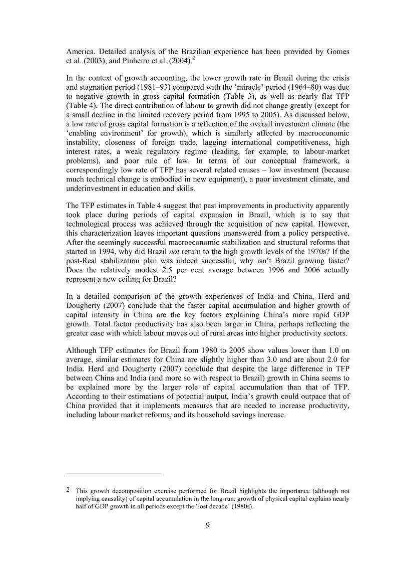
In the context of growth accounting, the lower growth rate in Brazil during the crisis and stagnation period (1981–93) compared with the ‘miracle’ period (1964–80) was due to negative growth in gross capital formation (Table 3), as well as nearly flat TFP (Table 4). The direct contribution of labour to growth did not change greatly (except for a small decline in the limited recovery period from 1995 to 2005). As discussed below, a low rate of gross capital formation is a reflection of the overall investment climate (the ‘enabling environment’ for growth), which is similarly affected by macroeconomic instability, closeness of foreign trade, lagging international competitiveness, high interest rates, a weak regulatory regime (leading, for example, to labour-market problems), and poor rule of law. In terms of our conceptual framework, a correspondingly low rate of TFP has several related causes – low investment (because much technical change is embodied in new equipment), a poor investment climate, and underinvestment in education and skills.
The TFP estimates in Table 4 suggest that past improvements in productivity apparently took place during periods of capital expansion in Brazil, which is to say that technological process was achieved through the acquisition of new capital. However, this characterization leaves important questions unanswered from a policy perspective. After the seemingly successful macroeconomic stabilization and structural reforms that started in 1994, why did Brazil not return to the high growth levels of the 1970s? If the post-Real stabilization plan was indeed successful, why isn’t Brazil growing faster? Does the relatively modest 2.5 per cent average between 1996 and 2006 actually represent a new ceiling for Brazil?
In a detailed comparison of the growth experiences of India and China, Herd and Dougherty (2007) conclude that the faster capital accumulation and higher growth of capital intensity in China are the key factors explaining China’s more rapid GDP growth. Total factor productivity has also been larger in China, perhaps reflecting the greater ease with which labour moves out of rural areas into higher productivity sectors.
Although TFP estimates for Brazil from 1980 to 2005 show values lower than 1.0 on average, similar estimates for China are slightly higher than 3.0 and are about 2.0 for India. Herd and Dougherty (2007) conclude that despite the large difference in TFP between China and India (and more so with respect to Brazil) growth in China seems to be explained more by the larger role of capital accumulation than that of TFP. According to their estimations of potential output, India’s growth could outpace that of China provided that it implements measures that are needed to increase productivity, including labour market reforms, and its household savings increase.
2 This growth decomposition exercise performed for Brazil highlights the importance (although not implying causality) of capital accumulation in the long-run: growth of physical capital explains nearly half of GDP growth in all periods except the ‘lost decade’ (1980s).
10
4 Structural factors impacting efficiency and growth
In early 2005, Brazil adopted an orthodox macroeconomic policy framework that encompassed fiscal discipline, a floating exchange rate, and inflation-targeting. Although Brazil has achieved stability, it has not grown at rates as rapid as those of China and India.
4.1 Trade orientation and growth
Many studies of growth have found an important relationship between trade orientation and growth. The acceleration of growth is often linked to export expansion, especially from the industrial sector. Using sectoral data for manufacturing and extractive industries Bonelli (1992) studied the relationship among TFP, output growth, and trade orientation for the period preceding trade liberalization. As might be expected, Bonelli finds a positive association between export expansion and rates of productivity change as estimated by TFP growth. Export expansion followed a programme of trade liberalization that contributed substantially to the growth in nearly all industries from 1980 to 1985 despite the larger crisis that then enveloped the economy.
Periods of increased TFP (and corresponding growth) can also be linked to lower import tariffs that effectively reduced protection for domestic industries but coincided with productivity gains for the sector overall. Ferreira and Rossi (2003) provide empirical analysis on how trade liberalization that began in the 1980s affected industrial sector productivity growth. By analyzing the periods before and after trade liberalization, they show that TFP grows faster at lower rates of protection. The findings are less conclusive for countries such as Chile, Mexico, and Argentina. But for Brazil at least, a strong case can be made that trade liberalization had a positive impact on TFP and growth.
Moreira (2004) examined the relationship between trade liberalization and increased productivity, also concluding that liberalization leads to stronger growth. His estimates suggest that the productivity increases following Brazil’s trade liberalization in 1988–90 were actually larger than those in Mexico following NAFTA. He attributes subsequent slow growth to the lack of an aggressive trade policy. As expected, the positive effects of liberalization on productivity were mainly concentrated in the export sector with limited spillover effect on the rest of the economy.
The changing structure of exports is also quite revealing when Brazil, over the past 20 years, is compared with China and India. As shown in Table 5, in Brazil there has been a reduction of 11 per cent in the share of food exports. Most of that decrease has been made up by an increase in the share of manufactures from 44 per cent to 54 per cent. However, the share of manufactures in Brazil’s total merchandise exports appears relatively small when compared with 70 per cent for India, and 92 per cent for China. Over the same period, India’s increase in the share of exports of manufactures was 12 per cent, but China’s was an impressive 66 per cent.
11
Table 5: Changing structure of merchandise exports between 1985 and 2005
Food Agricultural
raw materials Fuels Ore and metals Manufactures
1985 2005 1985 2005 1985 2005 1985 2005 1985 2005
Brazil 37 26 3 4 6 6 9 10 44 54
China 13 3 5 1 26 2 2 2 26 92
India 28 9 5 2 6 11 8 7 58 70
Source: World Bank. World Development Indicators.
4.2 The constraining effect of the public sector
Many observers over the past two decades have pointed to the large size of Brazil’s public sector as a growth constraint, particularly as it affects both the cost of capital and high taxes.
From 1950 to 1980 – a period of high growth and boom – the public sector was the main agent for investment and the chief catalyst of growth in Brazil. However, with the fiscal weakening and debt crisis of 1982, the government’s capacity to invest was reduced substantially. At the same time, the private sector investment was unable to fill the gap, in part because it was held back by high interest rates and high taxes, related in turn to the large size of the government sector.
Explanations differ as to why the Brazilian economy slowed so dramatically in the 1980s and failed to recover its previous dynamism. Yet there is a growing consensus that the size of the government has been – and continues to be – an important factor. Using consolidated tax revenues as a simple proxy for size of government, Brazil has the largest government (relative to GDP) among large middle-income economies (including China and India, but also Argentina, Mexico, and Russia) and larger than economies that have entered the high-income category.
In addition to the distortions introduced by heavy taxation (especially in the case of Brazil), large government size in Brazil has resulted in a significant increase in government consumption and the corresponding contraction in public and private investment. The exceedingly large public sector results in high taxes, high interest rates, and lower infrastructure investment, all of which impede efficient resource allocation (especially in the use of technology), and hence, growth.
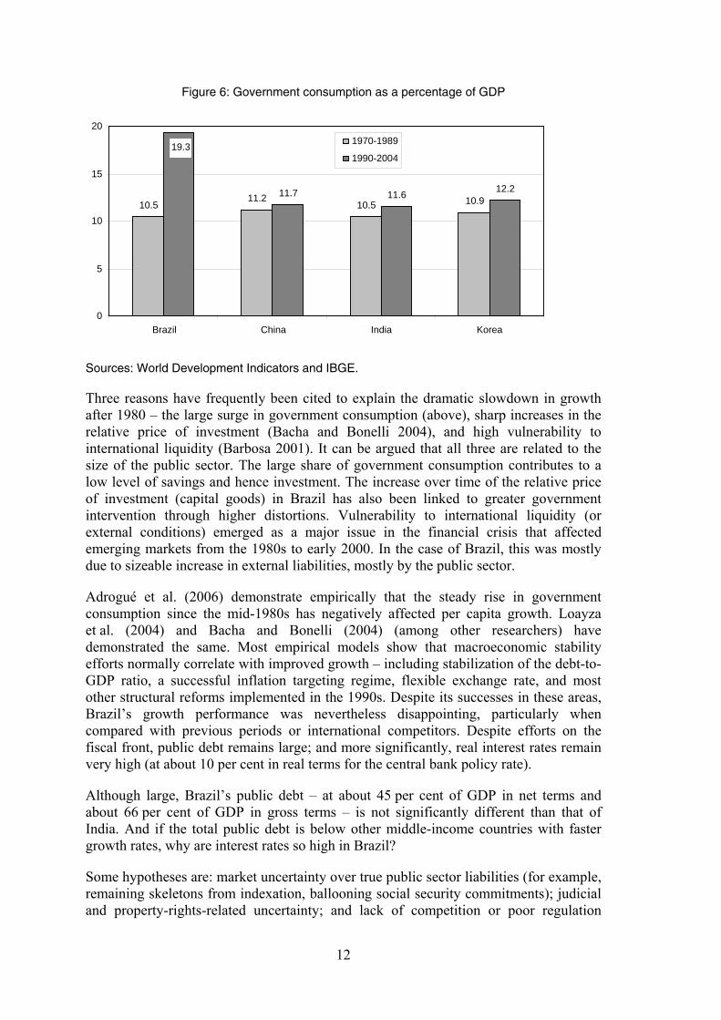
To analyse comparable figures of government size, we look at the relative size of government consumption (so as to eliminate investment) in Figure 6. The first column shows that since the 1988 Constitution (at which time government spending began to rise substantially), Brazil nearly doubled government consumption as a percentage of GDP. In contrast, government consumption rose modestly in China and India.
12
Figure 6: Government consumption as a percentage of GDP
Sources: World Development Indicators and IBGE.
Three reasons have frequently been cited to explain the dramatic slowdown in growth after 1980 – the large surge in government consumption (above), sharp increases in the relative price of investment (Bacha and Bonelli 2004), and high vulnerability to international liquidity (Barbosa 2001). It can be argued that all three are related to the size of the public sector. The large share of government consumption contributes to a low level of savings and hence investment. The increase over time of the relative price of investment (capital goods) in Brazil has also been linked to greater government intervention through higher distortions. Vulnerability to international liquidity (or external conditions) emerged as a major issue in the financial crisis that affected emerging markets from the 1980s to early 2000. In the case of Brazil, this was mostly due to sizeable increase in external liabilities, mostly by the public sector.
Adrogué et al. (2006) demonstrate empirically that the steady rise in government consumption since the mid-1980s has negatively affected per capita growth. Loayza et al. (2004) and Bacha and Bonelli (2004) (among other researchers) have demonstrated the same. Most empirical models show that macroeconomic stability efforts normally correlate with improved growth – including stabilization of the debt-to-GDP ratio, a successful inflation targeting regime, flexible exchange rate, and most other structural reforms implemented in the 1990s. Despite its successes in these areas, Brazil’s growth performance was nevertheless disappointing, particularly when compared with previous periods or international competitors. Despite efforts on the fiscal front, public debt remains large; and more significantly, real interest rates remain very high (at about 10 per cent in real terms for the central bank policy rate).
Although large, Brazil’s public debt – at about 45 per cent of GDP in net terms and about 66 per cent of GDP in gross terms – is not significantly different than that of India. And if the total public debt is below other middle-income countries with faster growth rates, why are interest rates so high in Brazil?
Some hypotheses are: market uncertainty over true public sector liabilities (for example, remaining skeletons from indexation, ballooning social security commitments); judicial and property-rights-related uncertainty; and lack of competition or poor regulation
11.2 10.5 10.9
11.7 11.6 12.2 10.5
19.3
0
5
10
15
20
Brazil China India Korea
1970-1989
1990-2004
13
within the financial sector. High public sector consumption (the Brazilian government has become a net dis-saver since the 1980s) is a leading factor in the relatively low level of savings and investment. This helps to explain why the inter-temporal price of consumption, namely the real interest rate, is so high. A large government burden from high consumption (and low savings and investment) is interrelated with high taxes and high interest rates.
Large government consumption also negatively impacts government investment in infrastructure. Gomes et al. (2003) and Adrogué et al. (2006) show empirically that despite all the efforts on the macroeconomic front, the sharp reduction in government investment during the 1990s and after 2000 has been a major factor in disappointing growth rates. Weak telecommunications, poor roads, inefficient ports, unreliable air transportation, questions on energy sustainability, and unequal access to water are all obvious obstacles to strong trade, commerce, and business.
An important difference needs to be pointed out in relation to India and its large public debt (explained by an accumulation of large fiscal deficits). In fact, India’s growth and its relative weak fiscal stance seem to contradict Brazil’s predicament. India has continued to grow with an ever increasing public debt, which reached more than 80 per cent of GDP in 2005 compared to less than 50 per cent in 1980. In addition, fiscal difficulties have resulted, similarly to Brazil, in cuts in government investment in infrastructure (after the 1991 crisis and adjustment, government capital expenditure was cut by 3 per cent of GDP). According to Pang et al. (2007), despite its fiscal difficulties India has remained fundamentally solvent as the loss of government revenue was, in part, due to the implementation of structural reforms that were growth-promoting. Government investment as a per cent of GDP declined from 6 per cent in the 1980s to 3 per cent in the 1990s while private investment as a per cent of GDP rose from about 12 per cent to about 23 per cent over the 25 years ending in 2005. Finally, the mostly domestic composition of public debt did not result in an external debt crisis as in the Brazilian case, and the implicit solvency has also resulted in comparatively lower interest rates that have contributed to the growth of the private sector.
Over the last three decades, China has downsized the public sector to the extent that it now has a more modest government size and social welfare policy than India or Brazil. Nonetheless, the provision of infrastructure spending by the government is significantly larger in China than either in India or Brazil. This has the potential of providing positive externalities for the private sector by providing a ‘crowding-in’ effect, promoting investment and growth.
5 The model
We use the stochastic production frontier to compare economic efficiencies of Brazil, India and China, where economic efficiency measures the gap between potential and actual outputs for a given input combination and technological factor. The stochastic production frontier models include non-positive error terms that capture production inefficiencies in each country and random residuals that account for the stochastic characteristic of the production functions. Going beyond measuring the contributions of factors of production and technology to growth, the results presented here suggest that a substantial improvement in economic efficiency in China and India over the last three decades help explain the more rapid growth of these countries relative to Brazil.
14
Following Aigner et al. (1977) and Meeusen and Van den Broeck (1977), and Battese and Coelli (1992), we consider a general stochastic production frontier function of the form:
)exp( itititit AXY νεβ −= (1)
where Yit is the real GDP, A is a Hicks-neutral constant rate of productivity growth, Xit is a (1 × k) vector of the inputs, β are unknown parameters, εit are individually, identically and normally distributed error terms ),0( 2
εσN , and υit are non-negative random errors that capture country-specific production inefficiency. The production frontier is the maximum output that can be achieved for a given set of inputs and is subject to a random, mean-zero variation captured by the error term εit
outside the control of a given country.
Technical efficiency of the ith country at time t is then measured by:
1ˆ
0 ≤=≤it
itit Y
Ye (2)
As eit 1, the ith country approaches its stochastic production frontier, reflecting increased production efficiency. Setting ))(exp( Ttvv iit −−= δ , where δ is an unknown parameter to be estimated from data, allows for both time-invariant (δ=0, iit νν = ) and time-variant technical inefficiency. In this study, we only consider time-variant production efficiency as the assumption of constant production inefficiencies over a span of three decades is highly unrealistic.
We assume that the production inefficiency terms (υits) are individually and identically distributed following a truncated ),0( 2
υσN . Battase and Coelli (1992) allow inefficiency to change systematically over time by estimating δ from the data by setting
222νε σσσ += and )/( 222
νεν σσσγ += and estimating the model using the Davidson-Fletcher-Powell algorithm. As an alternative, Battase and Coelli (1995) propose stochastic frontier models for panel data with inefficiency effects that are determined by independent variables. Instead of estimating a constant inefficiency factor from the data, we use frameworks suggested by Kumbhakar et al. (1991) and Battase and Coelli’s (1995) to allow the inefficiency terms to be driven by a set of factors are considered to have a significant impact on production efficiency of a country that change over time and estimate stochastic frontier models with v = f(z) where z represents structural variables.
6 The data and estimation results
We use a panel data set consisting of 27 time series observations (1980-2006) across three countries of Brazil, China and India for a total of 81 observations to estimate a Cobb-Douglas production function with time-varying inefficiencies. Battese and Coelli (1992) showed that it is possible to estimate such a function with panel data with production inefficiency terms (υit) that are assumed to follow a truncated normal distribution.
15
More specifically, we estimate a Cobb-Douglas function of the form:
)()ln()ln()ln( 210 ititititit LKY νεβββ −+++= (3)
with inefficiency terms that are time-variant and follow a truncated-normal distribution. Following our discussions of the preceding sections, we explore country-specific factors that may affect predicted efficiencies in each country over time. We allow the inefficiency factor to be determined by structural variables that capture the role of the government in the economy, the openness of the economy to trade and the level of international competitiveness as measured by the real effective exchange rate defined as annual average index of the nominal effective exchange rate of the local currency with respect to six leading trading partners, deflated by relative consumer prices.
Country-specific, time-varying inefficiency terms, υit, are determined by:
),,( 321 zzzfit =ν (4)
where z1 is a proxy for the size of the government in the economy, z2 measures the openness of the economy to trade, and z3 is a proxy for a country’s international competitiveness.
The real GDP data is taken from the Institute of International Finance (IIF) databases. We use the perpetual inventory method to estimate the net capital stock (see, for example, OECD 2001). In this method, the capital stock at time t+1 is found by adding gross investment at time t to the capital stock at that time (Kt) net of depreciation (δ):
ttt KIK )1(1 δ−+=+ (5)
The investment variable used in equation (5) to construct a data series on capital stock used in estimating the Cobb-Douglas production function (equation 3) is from the Penn World Table (PWT, Version 6.2) of Heston et al. (2006). We used the World Bank’s total labour force data for the labour variable in estimating equation (3). A country dummy variable was also included in equation (3).
The independent variables used in equation (4) include the logarithm of the government share of real GDP (z1), the logarithm of the ratio of the sum of exports and imports relative to real GDP (z2) and the logarithm of the real effective exchange rate (z3). The underlying data for these three variables are drawn from the PWT. A dummy variable for Brazil’s low growth ‘lost decade’ of the 1980s was included in estimating equation (4).
The parameters in equations (3) and (4) are estimated by maximizing the log-likelihood function using the Davidson-Fletcher-Powell algorithm. Estimation results are summarized in Table 6. These results show that labour and capital have statistically significant positive impact on the output. Efficiency of production is adversely impacted by rising government consumption. The variable z2 has a statistically significant negative impact on the inefficiency term v, indicating higher economic efficiency for more open economies. Higher levels of international competitiveness as measured by the purchasing power parity (z3) contribute to more efficient economies (Table 6).
16
Table 6: Maximum likelihood estimates of error component frontier
Variable
Coefficient estimate
Standard error
t- statistics
Production model variables Constant -17.83 0.18 -97.14 Capital 0.58 0.01 76.67 Labour 1.31 0.01 156.50 Dummy 1.19 0.01 11.72
Structural model variables
Government consumption 0.02 0.00 5.16 Openness -0.01 0.00 -6.10 Real exchange rate 0.02 0.00 5.87 Dummy -0.14 0.04 -3.49
Notes: Log likelihood function = 89.68. Likelihood ratio test of the one-sided error = 40.66.
Estimates of economic efficiency as defined by equation 2 over the last 27 years are presented in Figure 7. Brazil’s production efficiency has been lower than those of China and India over the last three decades. Brazil’s efficiency was particularly low during the ‘lost decade’ of the 1980s. During that decade, China’s production efficiency began to improve substantially. By the end of the decade, China’s production efficiency had surpassed that of India while Brazil’s efficiency was well below that of China and India. Brazil has improved production efficiency substantially since the mid-1990s, narrowing its efficiency gap with China and India. India improved its production efficiency beginning in the late 1980s and appears to have closed its efficiency gap with China.
Figure 7: Economic efficiencies: Brazil, China and India 1980-2007
Comparing growth and economic efficiencies in Brazil, India and China over the last three decades, we conclude that the more rapid growth of India and China is explained, in part, by relatively more efficient production in these countries compared with Brazil. Economic efficiency in Brazil has improved substantially since the mid-1990s. Nonetheless, Brazil remains less efficient that China and India.
We related the differences in production efficiency to three structural factors that we identified in our discussion of Brazil’s growth experience as important contributors to growth. We have shown that, in general, reducing government consumption, increasing openness to trade and having a more competitive exchange rate are important variables explaining the differences in production efficiency over time.
18
References
Abreu, M., and D. Verner (1997). ‘Long-Term Brazilian Economic Growth 1930-94’. Development Centre of the OECD.
Aigner, D., C. A. Knox Lovell, and P. Schmidt (1977). ‘Formulation and Estimation of Stochastic Frontier Production Function Models’. Journal of Econometrics, 6(1): 21–37.
Adrogué, R., M. Cerisola, and G. Gelos (2006). ‘Brazil’s Long-Term Growth Performance: Trying to Explain the Puzzle’. Working Paper No. 06/282. International Monetary Fund, Washington, DC.
Bacha, L. E., and R. Bonelli (2004). ‘Accounting for Brazil’s Growth Experience – 1940-2002’. Texto para Discussão nº1018. IPEA.
Baer, W. (2001). The Brazilian Economy: Growth and Development. 5th edition. Westport, Connecticut: Praeger.
Barbosa, N. H. (2001). ‘International Liquidity and Growth in Brazil’. Center for Economic and Policy Analysis. Working Paper 2001.04. New School University.
Battese, G. E., and T. J. Coelli (1992). ‘Frontier Production Functions, Technical Efficiency and Panel Data: With Application to Paddy Farmers in India’. Journal of Productivity Analysis, 3(1-2): 153–69.
Battese, G. E., and T. J. Coelli (1995). ‘A Model for Technical Inefficiency Effects in a Stochastic Frontier Production Function for Panel Data’. Empirical Economics, 20(2): 325–32.
Bonelli, R. (1992). ‘Growth and Productivity in Brazilian Industries’. Journal of Development Economics, 39(1): 85–109.
Carneiro, D. (1999). ‘Crescimento Economico e Instabilidade no Brasil’. Texto para Discussao No. 410. Departamento de Economia, PUC-Rio.
De Gregorio, J. (1992). ‘Economic Growth in Latin America’. Journal of Development Economics, 39(1): 59–84.
Elías, V. J. (1992). Sources of Growth. A Study of Seven Latin American Economies. Fundación del Tucumán and International Center for Economic Growth.
Fajnzylber, P., and D. Lederman (1999). ‘Economic Reforms and Total Factor Productivity Growth in Latin America and the Caribbean (1950-1995)’. The World Bank. Policy Research Working Paper 2114 (May).
Ferreira, P. C., and J. L. Rossi (2003). ‘New Evidence from Brazil on Trade Liberalization and Productivity Growth’. International Economic Review, 44(4): 1383–1405.
Gomes, V., S. A. Pessôa, and F. A. Veloso (2003). ‘Evolução da Produtividade Total dos Fatores na Economia Brasileira: Uma Análise Comparativa’. Pequisa e planejamento econômico, 33(3): 389–434.
Herd, R., and S. Dougherty (2007). ‘Growth Prospects in China and India Compared’. The European Journal of Comparative Economics, 4(1): 65–89.
19
Heston, A., R. Summers, and B. Aten (2006). Penn World Table Version 6.2. Center for International Comparisons of Production, Income and Prices at the University of Pennsylvania.
Kumbhakar, S. C., S. Ghosh, and J. T. McGuckin (1991). ‘A Generalized Production Frontier Approach for Estimating Determinants of Inefficiency in US Dairy Farms’. Journal of Business and Economic Statistics, 9(3): 279–86.
Loayza, N., P. Fajnzylber, and C. Calderón (2004). ‘Economic Growth in Latin America and the Caribbean: Stylized Facts, Explanations, and Forecasts’. Working Paper No. 65. Banco Central de Chile.
Meeusen, W., and J. Van den Broeck (1977). ‘Efficiency Estimation from Cobb-Douglas Production Functions with Composed Error’. International Economic Review, 18(2): 435–44.
Moreira, M. M. (2004). ‘Brazil’s Trade Liberalization and Growth: Has it Failed? INTAL-ITD. Occasional Paper 24.
Nazmi, N. (2002). ‘Global Finance, Sovereign Risk and Economic Performance in Brazil’. The Quarterly Review of Economics and Finance, 42(5): 865–74.
Nazmi, N. (2007). ‘Financial Sector Reforms and Economic Growth in China’, in J. Chen and S. Yao (eds) Globalization, Competition and Growth in China. New York: Routledge.
Organization for Economic Cooperation and Development (OECD) (2001). ‘Measuring Capital: A Manual on the Measurement of Capital Stocks, Consumption of Fixed Capital and Capital Services’. Paris.
Pang, G., B. Pinto, and M. Wes (2007). ‘India Rising – Faster Growth, Lower Indebtedness’. Policy Research Working Paper WPS 4241. Washington: World Bank (June).
Perkins, D. H. (2007). ‘Asian Development Strategies, 1950-2006’. Processed. Harvard University (July).
Pinheiro, A. C., I. Gill, L. Servén, and M. Thomas (2004). ‘Brazilian Economic Growth, 1900-2000: Lessons and Policy Implications’. Inter-American Development Bank.
Prasad, E. (2007). ‘Is the Chinese Growth Miracle Built to Last?’ Mimeo. Cornell University (July). http://prasad.aem.cornell.edu/doc/new_papers/ChinaGrowth.pdf.
Wilson, D., and R. Purushothaman (2003). ‘Dreaming with BRICs: The Path to 2050’. Global Economics Paper 99. Goldman Sachs.
World Bank (2007). ‘Brazil: Knowledge and Innovation for Competitiveness’. Processed. (June).