ECONOMIC FACTORS AFFECTING HUMAN FERTILITY IN THE DEVELOPING AREAS OF SOUTH AFRICA by CHERYL DENISE FAIRLAMB Submitted in partial fulfilment of the requirements for the degree DOCTOR OF PHILOSOPHY in the Department of Agricultural Economics University of Natal Pietermaritzburg 1990
Transcript
ECONOMIC FACTORS AFFECTING HUMAN
FERTILITY IN THE DEVELOPING
AREAS OF SOUTH AFRICA
by
CHERYL DENISE FAIRLAMB
Submitted in partial fulfilment of
the requirements for the degree
DOCTOR OF PHILOSOPHY
in the
Department of Agricultural Economics
University of Natal
Pietermaritzburg
1990
I hereby certify that the work reported in this thesis, unless specifically indicated to the
contrary in the text, is my own original and unaided work.
~A~~ C.D. F AIRLAMB
\
ABSTRACT
The World Bank has expressed concern over the high population growth rates in sub-saharan Mrica.
South Africa's annual population growth rate in the traditional sector is 2,9 percent. This study
identifies the economic factors affecting family size choice to provide policy makers with a strategy for
reducing fertility.
A neoclassical utility framework was used to analyse linkages between family size decisions and socio
economic variables. Household utility for "child services" and "standard of living" was maximised
subject to the resource constraints of time, labour and income. A stratified sampling technique was
used to collect household data from illundi and Ubombo in KwaZulu. One hundred and seventy five
women in three occupational strata were interviewed. A static demand function for children was
estimated by multiple regression. The demand function was re-estimated within a simultaneous model
of family decision making which was estimated by two-stage least squares regression analysis. Dummy
dependent variables were estimated by probit analysis. Principal components analysis was used to
confirm the underlying theoretical linkages and discriminant analysis was used to distinguish users
from non-users of modern contraception.
Results show that child education, woman's opportunity cost of time and formal labour market partici
pation were negatively related to fertility reflecting a substitution from numbers of children (time
intensive goods) to fewer, more educated children (less time intensive) as opportunity costs rise.
Principal components confirmed that this substitution effect dominated the pure income effect as
lifetime family earnings increased even though children are normal goods.
Child labour and children's contribution to income ~ere positively related to fertility. These benefits
accrued mainly to rural people because in urban areas parents depend less on subsistence farming and
essential services (water and electricity supply) are provided.
Discriminant analysis showed that 47,7 percent of the respondents used contraception (including
abstinence and sterility). The most important reasons for use were for child spacing and the desire for
no more children. The latter reason was given by women who had completed fertility and young
women who wanted to avoid untimely pregnancy. The actions of the young women emphasise the
importance of opportunity cost which was further supported by positive relationships between woman's
current income, child education and contraceptive use.
Therefore strategies to reduce population growth rates should include improvements in education and
employment opportunities which would raise time costs for women. Provision of time saving devices
and essential services, and better pension and social security schemes would reduce the benefits from
children thereby reducing family size. For better community acceptance of contraception, the benefits
for child spacing and survival should be promoted.
ACKNOWLEDGEMENTS
I would like to express sincere thanks and appreciation to all who assisted my research. I am especially
indebted to the following people:
Professor W.L. Nieuwoudt, Head of the Department of Agricultural Economics, University of Natal,
who as my supervisor guided and supported me throughout; his encouragement was much
appreciated.
The HSRC which, through the Policy Research Unit, sponsored my research.
The institutions which allowed me to interview their employees namely Mjindi Cotton Scheme,
Division (Ulundi) and the KwaZulu Government Offices (Ulundi); without their consent my research
would have been impossible.
Mr J. Pretorius, Mr E. Le Roux and members of KwaZulu Department of Agriculture for their help
and support in obtaining permission for my studies in Ulundi, and special thanks to Duncan Stew~rt
whose advice, encouragement and hospitality can never be repaid.
To the Mjindi staff who were supportive in Jozini especially Steve Woodburne, Johan and Kelly Botha,
Dale and Sharee van den Aardweg, Piet van Vuuren and Roy Kiddie.
Sincere thanks also to Peter and Fiona Wakelyn for their advice and encouragement when times were
bleak; and to Captain Smith for accommodation in Jozini.
To colleagues and staff in the Agricultural Economics Department, University of Natal, especially Mike
Wheeler and Vlad Dushmanitch for their emotional support, taxi services and friendship. Finally
thanks to my family and my Creator.
LIST OF CONTENTS
CHAPTER
1
ABSTRACT
ACKNO~DGEMENTS
LIST OF CONTENTS
LIST OF TABLES
LIST OF FIGURES
LIST OF APPENDICES
INTRODUCTION
REVIEW OF ECONOMIC APPROACHES TO FERTILITY ANALYSIS
1.1 INTRODUCTION
1.2 THE PURE NEOCLASSICAL APPROACH
1.2.1 The Mincer Model
1.2.2 Freedman's Hypothesis on Relative Income
1.2.3 The Theory of Economics of Time
1.3 THE CHICAGO SCHOOL
1.4 THE SOCIOECONOMIC AND BEHAVIOURAL MODELS
1.4.1 The Supply of Children
1.4.2 The Demand for Children
1.4.3 Fertility Regulation
1.4.4 The Treatment of Tastes in Behavioural Models
PAGE
(i)
(v)
(v i)
( vii)
1
5
5
6
7
9
9
10
12
12
13
14
15
CHAPTER
1.4.4.1 Social Influence Groups (SIGs) and Background Characteristics
1.4.4.2 Income and Its Distribution
1.4.4.3 Social Norms
1.4.4.4 Social-psychological Approaches
1.5 SUMMARY AND CRITICAL OVERVIEW OF THE MICROECONOMIC ANALYSIS OF FERTILITY
2 FORMULATION OF THE MODEL
2.1 INTRODUCTION
2.2 SPECIFICATION OF THE MAJOR RELATIONSHIPS
2.2.1 Income and Price Effects
2.2.2 Measurement of Income
2.2.3 Education (Technology)
2.2.4 Tastes and Demographic Variables
2.3 A MICROECONOMIC MODEL OF FERTILITY
2.3.1 General Formulation
2.3.2 An Adaption to a Developing Country's Situation
2.3.2.1 An Appropriate Fertility Model
2.3.2.2 Parametric Changes and Demand Analysis
3 SAMPLING AND ESTIMATION TECHNIQUES
3.1 THE SAMPLING TECHNIQUES
3.2 THE SURVEY
ii
PAGE
15
17
18
19
24
28
41
42
47
57
CHAPTER
3.3
3.2.1 Introduction
3.2.2 Description of the Survey Areas
3.2.2.1 Ubombo Magisterial District
3.2.2.2 Ulundi: An Urban Area
3.2.3 Methodology
3.2.4 Interview Technique
3.2.4.1 Questionnaire
ESTIMATION TECHNIQUES
3.3.1 Regression Analysis
3.3.1.1 Mutiple Regression
3.3.1.2 Simultaneous Equation Models
3.3.1.3 Two-Stage Least Squares Regression Analysis
3.3.2 Probit Analysis
3.3.3 Principal Components
3.3.4 Discriminant Analysis
4 THE EMPIRICAL MODEL AND RESULTS
4.1 DESCRIPTIVE STATISTICS
4.1.1 The Measure of Fertility
4.1.2 Income Measures
4.1.3 Opportunity Cost of Woman's Time
4.1.4 Child Quality as an Estimate of Child Costs
4.1.5 Child Benefits
4.1.6 Tastes for Children and the Status Effect
4.1.7 Control Variables
iii
PAGE
EX>
EX>
EX>
00
01
00
73
75
71
71
71
8)
84
ffi
ffl
91
91
CHAPTER
4.1.8 Variables Associated with Contraception
4.2 RESULTS OF REGRESSION ANALYSIS
4.2.1 Effect of Intercept Changes on Regression
4.2.2 Regressions with full Interaction Terms
4.3. RESULTS OF PRINCIPAL COMPONENTS ANALYSIS
4.4
4.5
4.3.1 The Substitution Effect
4.3.2 The Income Effect
4.3.3 Investment in Children
4.3.4 Summary of Principal Components Analysis
RESULTS OF THE SIMULTANEOUS MODEL
4.4.1 Structural Equations of the Simultaneous Model
4.4.2 Derivation of the Instrumental Variables
4.4.3 Results of the Simultaneous Model of Family Size Decision-making
DISCRIMINANT ANALYSIS
DISCUSSION AND CONCLUSIONS
SUMMARY
REFERENCES
APPENDICES
iv
PAGE
10i
10i
1m
1m
1m
liD
112
118
LIST OF TABLES
TABLE
2.1
4.1
Mean total household income by source for KwaZulu (1988)
Means of quantity of children, income, costs and education of the different family members by strata in KwaZulu, 1988.
4.2 Permanent Income Estimated by Principal Component Analysis
v
PAGE
51
79
4.3 Means of child education, child help and control variables by strata in KwaZulu, 1988 88
4.4 Index of child help variables constructed by principal component analysis
4.5 Index of status variables constructed by principal component analysis
4.6 Demand for children (NOC), KwaZulu, 1988: on all proposed explanatory variables, restricting dummies to intercept changes alone
4.7 Demand for Family Size, KwaZulu, 1988: predictor variables' t-value > 1, and dummies are restricted to intercept changes alone
4.8 Construction of interaction variables: each row is multiplied by each column
4.9 Demand for family size, KwaZulu, 1988 (including interaction variables)
4.10 Results of principal component analysis
4.11 A Priori Prediction of Coefficient Signs in the Econometric Model of Fertility
100
4.12 Results of the Simultaneous Model of Family Size Decision-making (Data were collected in 1988). 114
4.13 The discriminant function showing variables which best distinguish between users and non-users of contraception (n = 170) 121.
LIST OF FIGURES
FIGURE
1.1 Social influence groups and the demand for children
1.2 Hypothetical trends in household fertility
3.1 Map of Myeni ward showing the blocks from which "housewives· in Ubombo were chosen
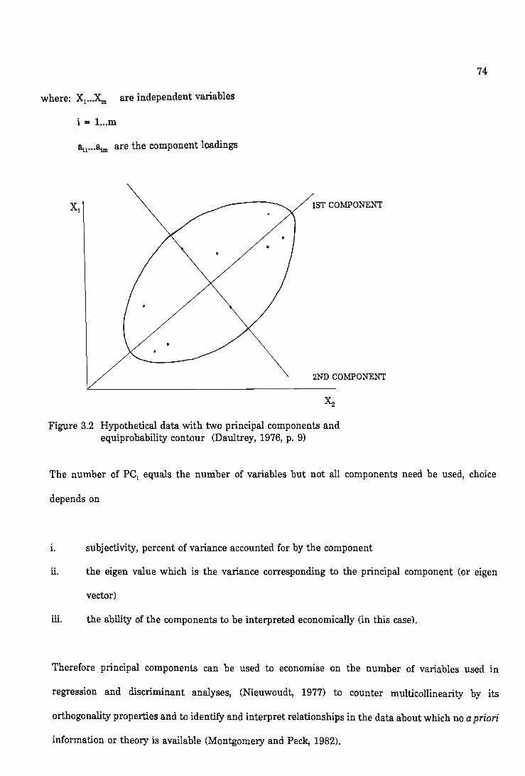
3.2 Hypothetical data with two principal components and equiprobability contour
vi
PAGE
17
19
74
LIST OF APPENDICES
APPENDIX
A.1 QUESTIONNAIRE
A.2 LIST OF VARIABLES
A.3 DESCRIPTIVE STATISTICS
A.3.1 Means and standard deviations of the child help variables (KwaZulu, 1988)
A.3.2 Means and standard deviations of the ownership of assets (KwaZulu, 1988)
A.3.3 Summary of reasons given for use or non-use of contraception: means and associated standard deviations reported for 175 cases
vii
PAGE
14i
152
152
1
INTRODUCTION
High population growth rates have been a major factor inhibiting economic development in third world
countries. Africa has been the focus of world attention in recent years because its growth rate has
increased from 2,1 percent per annum in 1950 to 2,9 percent in 1980 and is estimated to grow
approximately 3 percent annually until the end of the century (United Nations, 1981). Rates have
exceeded four percent per annum in Kenya, Mozambique, and the Ivory Coast, with others like
Zimbabwe expected to join them by the turn of the century (World Bank, 1984).
South Africa's growth rate during 1970 - 2000 is estimated as being 2,5 percent per annum (University
of South Africa, 1989). The popUlation of 37 532 000 is made up of 13,5 percent Whites, 8,6 percent
Coloureds, 2,6 percent Asians and 75,3 percent Africans. The estimated population growth rates for
the different racial groups show that the highest growth rate of 2,9 percent per annum (1970 - 2000)
is for Africans, Coloureds, Asians and Whites having growth rates of 1,9, 1,8 and 1,1 percent per
annum respectively (University of South Africa, 1989). Within the African sector the Development
Bank of Southern Africa (1987) estimates that 46 percent of the popUlation is younger than fifteen
years. This skewness causes a momentum effect which keeps birth rates high in spite of decreasing
growth rates; the World Bank (1984) estimates that it can take 50 - 75 years for the momentum to
adjust to growth rate declines.
These statistics have serious implications for development in South Africa. Provision of education,
housing, employment, health care and food production are a few of the areas that need attention. For
this reason in March 1984 Cabinet launched the PopUlation Development Programme (PDP), whose
aim was to establish an equilibrium between population size and available resources (van der Kooy,
1990). Future availability of natural resources, the country's economic and social potentials and
possible governmental programmes were to be considered. The PDP, having acted on two investi
gations commissioned by the President's Council, found that South Africa can only accommodate 80
million people (van der Kooy, 1990). An economic growth rate of 4,5 percent per annum for 1980 -2000
2
would only create 12 million jobs, 6 million short by the year 2000 for no unemployment to exist. At
an economic growth rate of 3,1 percent per annum, no more than 10 million jobs would be available
while a rate closer to 2,5 percent appears achievable. It is therefore imperative that economic
conditions of traditional1 households associated with smaller family sizes should be studied in order
to facilitate fertility declines and the raising of living standard potentials.
Family planning strategies have met with certain success in Taiwan, Korea, Singapore and China but
in Africa they appear to be less effective. Dow and Werner (1981) in Kenya found that although 64,2
percent of women knew about modern contraception, those who were using it did so to complement
and maintain rather than change and reduce their fertility aspirations. This exposes possibly the most
fundamental problem of family planning strategies, the fact that they concentrate on the symptoms
rather than the cause of high fertility. In Taiwan, focus was placed on motivating couples to reduce
fertility by a comprehensive marketing strategy which explained the problems of rapid growth and the
benefits of small family sizes. Taiwan coupled this campaign with inexpensive and readily available
contraception and has achieved the most rapid declines in population growth rates in the world
(Development and Communication Consultants, 1990).
In South Africa it is important to provide a comprehensive popUlation programme that motivates
people to reduce their family size preferences. This study was undertaken to consider how a long term
approach to decreasing desired family size might be achieved. Emphasis is placed on the underlying
economic factors affecting family size preferences which will allow policy makers to define an incentive
structure encouraging couples to regulate their fertility. It is important, though, to consider the social
and cultural aspects as well and to provide shorter term strategies.
Historically reduced popUlation growth has taken place as development proceeds suggesting that socio
economic conditions play an important role in family expectations and decisions. Thus, much of the
Traditional throughout this thesis refers to the African sector of the population including the National States and TVBC countries. It must be distinguished from traditional people within the African sector.
3
economic literature on the subject has focused on a neoclassical framework of utility maximisation in
an effort to derive a "demand curve" for children (Willis, 1971, 1973; De Tray, 1973, 1978; Michael,
1975; Dusenberry, 1960; and Easterlin, 1961, 1969).
Chapter one deals with the different approaches to the theory offamily size decision-making, critically
describing the differences between neoclassical, Behavioural and Chicago School approaches. Chapter
two formulates the empirical model within the Chicago School paradigm. The demand curve for
children is derived within a simultaneous model of family decision-making together with demand
curves for child quality and woman's work participation. An estimate of permanent income and
woman's opportunity cost are included.
Chapter three describes data collection and estimation techniques. Household data were collected from
the Ubombo and Mahlabathini magisterial districts in KwaZulu. The former area was considered
typically rural and Ulundi, in Mahlabathini was selected as an urban area. The sample was stratified
by woman's occupation to ensure variability in woman's education and opportunity cost of time
variables. One hundred and seventy eight women were interviewed in the following three strata,
professional women (stratum 1), industrial workers (stratum 2), and women not formally employed
(stratum 3).
Chapter four reports the descriptive statistics of the database, after which results are presented. Single
equation demand functions for children will be estimated with ordinary least squares regression. The
demand function will then be re-estimated in a simultaneous system using two-stage least squares
regression with probit analysis to estimate dummy dependent variables. Principal components analysis
4
will be used to form indices where necessary and to confirm the theoretical linkages. Since family
planning is considered to be an important short term strategy for fertility reduction a discriminant
analysis will be used to distinguish users from non-users of modern contraception. Finally results will
be discussed with a view to promoting a more balanced strategy for policy makers in their attempt at
reducing population growth rates.
5
CHAPTER 1
REVIEW OF ECONOMIC APPROACHES TO FERTILITY ANALYSIS
1.1 INTRODUCTION
Malthus,as early as 1798 postulated that socioeconomic variables affected family size choice. He was
primarily concerned that as incomes increased, population would outstrip food production because
children were considered normal goods, thereby creating critical food shortages. Historically though,
the reverse is true, that is as nations become more affluent with higher per capita incomes, population
growth rates have declined inferring that children are inferior goods. This prompted analysis in the
area of human fertility amongst economists in the early sixties, who intuitively felt that other economic
or social factors caused the apparent negative relationship between income and fertility. They
suggested that fertility behaviour was linked to consumption and was a result of choice rather than
chance implying that decisions about having children reflect the behaviour of a rational utility
maximising decision maker. These postulates allowed the use of microeconomic theory to explain
fertility behaviour (Bagozzi and Van Loo, 1978; Schultz, 1973). Schultz (1974, p.4) proposed that the
"analytical core of fertility studies rests on the economic postulate that the reproductive behaviour of
parents is in large part a response to the underlying preferences of parents for children. Parents
respond to economic considerations in the children they bear and rear equating the marginal sacrifices
and satisfactions from children in arriving at a value of children to them. Thus the analytical key in
determining the value of children to their parents is in the interactions between the supply and
demand factors that influence these family decisions." This afforded theoretical models which were
used to explain the apparent paradox that children were inferior goods. The models originated mostly
from the works of Leibenstein (1957), Becker (1960, 1965), and Lancaster (1966a, 1966b) and have
become the basis of the following different approaches to fertility analysis.
a. The Pure Neoclassical Approach
6
b. The Chicago School
c. Socioeconomic and Behavioural Models
1.2 THE PURE NEOCLASSICAL APPROACH
Neoclassical consumer theory lends itself to the study of fertility because it is based on the assumption
of a rational utility maximiser. Decision makers, or parents in this case, are supposed to behave as if
they maximise their utility function subject to certain, given, nonstochastic constraints. Constraints
include prices of goods and services and income, where income is specified as equal to a given budget
(with savings and wealth excluded). From this maximisation demand curves for the individual goods
can be derived and the sensitivity of the solution checked by comparative statics. However a major
limitation of this approach is that it is not a dynamic process, as shown by Becker's model in 1960.
He assumed that a husband and wife make a single joint decision at the outset of marriage, about the
quantity of children, expenditures per child (or quality) and the standard of living of the household.
The couple maximises their utility between children and other goods and services which allows a
demand function for number of children to be derived as a function of the prices of other goods and
services, and the level of money income. The price of children is expressed in the terms of prices of
other goods both complements to and substitutes for children and is therefore, not included in the
demand function but rather an outcome of it (Bagozzi and Van Loo, 1978, p.200).
Becker postulated the negative relationship between money income and number of children was due
to differential knowledge of contraception. Better educated couples with higher incomes have more
knowledge about reducing the number of unintended births, thereby converting a positive income effect
on desired fertility to a negative income relationship with actual fertility (Becker, 1960, p.220).
Becker's model however, besides being static, did not satisfactorily explain the negative relationship
between income and fertility. Therefore other writers extended his basic model to improve on these
areas. Mincer (1963) and Freedman (1963) were two major contributors in this sense.
7
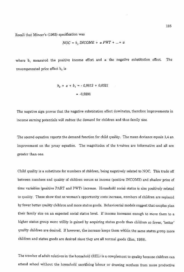
1.2.1 The Mincer Model
Generally Mincer (1963, p.67) was concerned with specification bias in economic models because of
"easily overlooked or misunderstood price variables". Prices in cross-sectional studies, were usually
assumed to be constant, but Mincer suggested that there were specific costs which varied amongst
individuals and should not be left out. Consumer's time and labour, being complementary resources
are examples of such costs. Mincer suggested the most important of these was opportunity cost of
time, which at the margin is linked to the wage rate, and consequently positively related to income.
Thus he defined price as:
p =p + c
where: p is the market selling price
c is the opportunity cost of time
The relative size of these two components differs by commodities and individuals. Usually c is assumed
to be negligible; at the other extreme (the case of leisure) p = 0 so P = c. The general demand
function becomes:
where: Yj is the consumption of the commodity by consumer i
is the income of consumer i
is the market price of good j
is the opportunity cost to consumer i of good j
is the error term for consumer i
Even if the PjS are fixed in cross-sectional studies, the cijs are not. If the cijs are a function of the wage
rate their omission will bias the estimate of b. He illustrated the effect of opportunity cost on fertility
8
by including a cost of children variable in his demand analysis. In his fertility model he stressed that
the decision to bear children is based on potential income flows or the long run anticipation of wealth.
Thus permanent income rather than current income is relevant for the choice problem. Therefore the
cost of bearing and rearing children is not current prices of market goods and services but rather the
opportunity cost of mother's time measured as her forgone wage earnings in the labour market. His
fertility demand function was
where: Xo
Xl
is the fertility variable
is husband's income
is wife's full time earnings
is the level of contraceptive knowledge
This can be rewritten as
where: X, = Xl + X2 or potential family income
a = b2 - bl = > b2 = a + bl
Economic theory would predict a positive income effect (b 1 > 0), and a negative opportunity cost effect
(a < 0) but it does not predict the sign of b2, the uncompensated price effect. The sign of b2
depends
therefore on whether the positive income effect or negative substitution effect dominates. In the case
with rising permanent income, wife's time becomes more valuable, increasing her opportunity cost
causing the substitution effect to outweigh the income effect which results in a negative relationship
between income and family size.
9
Mincer's (1963) model improved on Becker's (1960) by including expectations on wife's full time
earnings thereby making it more dynamic and providing a more convincing reason for the negative
relationship between income and family size.
1.2.2 Freedman's Hypothesis on Relative Income
Deborah Freedman's (1963) model provided an alternative to Mincer's (1963) price of time variable by
suggesting that within a socioeconomic reference group, the cost of rearing children is related to
standard of living and norms of that group. Therefore, within each reference group the number of
children is positively related to family income; between social groups however, the number of children
is negatively related to income. If an increase in income moves a family from one social group to a
higher status one the cost of children, in terms of standard of living, becomes greater which means
fewer children are demanded. The social reference groups are determined by occupation, religion, place
of residence, income and other socioeconomic variables.
1.2.3 The Theory of Economics of Time
Although Mincer (1963) made important theoretical contributions to fertility analysis by including time
costs indirectly, his model failed to cope with the allocative role of the decision unit (family). The
family must not only maximise utility in consumption but must allocate household members' time and
goods through household production decisions. Becker (1965) addressed this problem by arguing that
each consumer good or service has a money price and involves indirect costs of:
i. acquiring goods and processing them in household production activities
ii. consuming final goods obtained from household activities.
Therefore if children are economic goods, the costs of an additional child include the direct costs of
bearing and rearing the child, and the indirect costs associated with the time and labour intensities of
10
the direct costs. The latter includes costs related to forgone job opportunities, reduced geographical
and social mobility of the parents, etc. and therefore reflect the "price" of children in terms of goods and
services that are complements to or substitutes for children.
The idea that household production activities lead to final consumption is the core of the "New
Approach" (Ron, 1980). The household uses market goods and time to produce basic commodities (or
fundamental goods) which are the true source of utility. Therefore the demand for market goods is
a derived demand and the utility maximised is for the fundamental goods which in the case of children,
is "child services" incorporating the Lancasterian characteristics of health, education, prestige and
number of children. Family size is now explained by the prices of these basic commodity components
and income.
The development of the household, general equilibrium model of fertility used extensively in the litera
ture (Willis, 1971, 1973; De Tray, 1973, 1978; Schultz, 1969, 1974 and Ben-Porath, 1973, 1977)
evolved from the integration of the "Economic Theory of Family Formation" (Leibenstein, 1957; Becker,
1960; Easterlin, 1961, 1969 and Mincer, 1963) with the "New Approach to Consumer Behaviour"
(Becker, 1965; Lancaster, 1966a, 1966b). Simultaneous determination of choices an family income,
woman's labour force participation and the quantity/quality trade off for children can be accom
modated. The extended framework presented the idea that utility is obtained indirectly from market
goods via the consumption of basic commodities. The latter are produced by the household using time
and market goods and services as inputs. Thus when applied to family size decision making, it recog
nises that children in fact generate both consumer satisfaction and investment-like qualities, thereby
incorporating both production and consumption relationships within the framework of household utility
maximisation (Ron, 1980).
1.3 THE CHICAGO SCHOOL
The Chicago school adapts the "New Approach" to provide a framework to a choice problem where
11
there is an individual decision maker. The following assumptions are made:
i. A household production technology exists which converts market goods and time into home
consumed fundamental goods.
ii. Families choose quantity of children based on their utility function.
iii. Their choice is constrained by the availability of time and wealth and the derived demand for
children is explained by income, relative prices (costs) and the parents' "tastes" for children.
The cost of children is defined by expenditures per child or child quality. Ron (1980) proposes that
quality can serve as a proxy for the value of time for child care which is positively related to labour
income. Therefore this framework implicitly incorporates the reasons proposed by Becker (1965),
Mincer (1963) and Freedman (1963) for a negative relationship between income and family size.
Becker and Lewis (1973) posited that child quality and child quantity are substitutes varying directly
with expenditures of time and money. They further proposed that the income elasticity with respect
to child quality is greater than that with respect to numbers of children suggesting that higher income
earners will have fewer but higher quality children. Consequently, the cost of a child is associated with
the rise in the price of human time which historically has been increasing with rising wage rates.
Therefore as opportunity costs of child care have risen quality (which is less time intensive) has been
substituted for numbers of children, resulting in higher average utility per child expressed by higher
expenditures per child.
The Chicago School, following the neoclassical approach regards parents' tastes as a ceteris paribu.s
condition because economic theory fails to provide a way of modelling taste formation. As Michael and
Becker (1973) put it "for economists to rest a large part of their theory of choice on differences in tastes
is disturbing since they admittedly have no useful theory of tastes from any other discipline in the
social sciences since none exists" (quoted by Ron, 1980, p.15). Therefore followers of the Chicago school
expect tastes to be "stable over time and similar amongst people" (Stigler and Becker, 1977, p.76) and
thus are best incorporated as a disturbance term to explain residual error within the model (Robinson,
12
1979). However writers ofthe behavioural models reject the assumption that people are homogeneous
in preferences and propose that proxies like background characteristics, social pressure or psychological
needs should be used to explain fertility as well (Easterlin, 1969; Leibenstein, 1974; Turchi, 1975;
Bulatao and Lee, 1983).
1.4 THE SOCIOECONOMIC AND BEHAVIOURAL MODELS
Later ideas summarised by Bulatao and Lee (1983) on the methods to approach fertility analysis
provide a much boarder framework than that proposed by either the neoclassical or Chicago
approaches. This framework incorporates all aspects affecting fertility and can be seen as an integrated
approach. The decision unit here is the couple or household and all factors, including social influences,
must affect this unit in some way. Because fertility involves both biology, influenced by cultural
practices and social taboos, and individual choice which is strongly influenced by economic and social
conditions, the basic constituents of study are broken down into three major components following
Easterlin (1975, 1978) and are
i. the supply of children
11. the demand for children
iii. fertility regulation
1.4.1 The Supply of Children
The supply of children is defined by Bulatao and Lee (1983) as the number of surviving children a
couple would have if they made no deliberate attempt at limitation, or as Bulatao and Lee (1983, p.3)
suggest the "biocultural potential for surviving children". This is similar to the demographic definition
of "natural fertility" which Henry (1953) described as the "fertility of a human population that makes
no deliberate effort to limit births". Although theoretically correct it is extremely difficult to measure,
and supply is approximated by a family of age schedules of fertility.
13
Because natural fertility depends partly on cultural practices relating to such behaviours as intercourse,
abstinence, and breast feeding, it varies widely amongst populations, and is measured by the average
interval between births and the length of the reproductive span. Five major factors affecting these can
be identified.
i. Postpartum infecundability: conception and birth interrupt a women's normal pattern of
ovulation. How long after birth this interruption lasts depends largely on breast feeding
practices, which are often dependent on cultural norms.
ii. The waiting time to conception: is the period from first postpartum ovulation to conception.
iii. Intrauterine mortality: a substantial number of pregnancies end prematurely and therefore
effectively lengthen the interval between births.
iv. Permanent sterility
v. Entry into the reproductive span: this starts at the age of menarche and puberty for females
and males respectively. However these ages are usually less important than the ages at
marriage.
The first three of these factors influence the interval between births and the last two define the
reproductive span. Combined with survival chances these five factors determine the potential number
of children a couple can have.
1.4.2 The Demand for Children
Demand represents the number of children a couple desires as opposed to the potential number they
can have. By definition, these desires do not consider supply or the possibility of fertility regulation.
Other factors which may affect demand include gender preferences, birth spacing desires, the optimal
level of education children should receive etc. Thus demand is seen as an interplay between tastes for
children and constraints on the couple. The constraints which are emphasized by neoclassical writers
are mostly objective economic ones, but tastes are subjective and are "partly captured in the couples'
14
perceptions of the values and disvalues of children"; these perceptions, though more difficult to
measure, "are more immediately relevant to demand" (Bulatao and Lee, 1983, p.6). These issues will
be discussed more fully in a later section.
1.4.3 Fertility Regulation
For demand to be effective, there must be some way to make a couple's choice effective; fertility
regulation covers all their methods of doing so. Yet regulation always involves some costs, either direct
economic costs or psychological ones, which a couple must weigh up before decisions are made.
Fertility regulation includes contraception, induced abortion, infanticide, and to a lesser extent
abstinence or prolonged breast feeding. The costs involved comprise monetary costs, inconvenience,
embarrassment, guilt, the effort in getting the required information and using it, and lastly psychic or
social costs such as fear of being seen at family planning.
For a couple to use contraception of any form they must weigh up the relative levels of supply and
demand, and if supply exceeds demand, the costs involved in regulation. Hence only if a couple's
supply is greater than demand, and the motivation to regulate outweighs the cost of doing so, will a
couple even consider regulation. Therefore in this rather broad framework, supply influences demand
in an indirect way through the fertility control component which means that these functions can not
be considered to represent true economic demand and supply curves. Although this all-encompassing
framework allows more specific model formulations to be included, the behavioural models generally
are not as rigorous as neoclassical ones because of their emphasis on tastes. It is however important
to consider the attempts to incorporate tastes specifically on the demand side as this component has
the greatest potential for policy makers.
15
1.4.4 The Treatment of Tastes in Behavioural Models
Ron (1980, p.16) wrote that behavioural models try to explain fertility by "linking the process of
individual utility maximisation to social-behavioural variables such as norms, externalities among
various social groups and background characteristics." The result is that the demand function for
children emphasizes the relationship between fertility and relative income (as did Freedman, 1953),
and/or distribution rather than income per se. Therefore the core of these models is the assumption
that preferences (or tastes) are not static but shift in time and across social groups. Hence tastes are
explicitly considered by allowing socio-psychological factors, used as proxies for tastes, to enter the
model. These factors, such as peer group pressure, social status and other background variables which
explain taste formation, replace the rationale that the quantity-quality trade off interprets the negative
relationship between income and family size. Ron (1980) classified these models according to the
following behavioural dimensions:
i. the effects of social influence groups (8IGs) and the role of background characteristics
ii. income and its distribution
iii. the influence of normative determinants on fertility
iv. the integration of social-psychological factors
1.4.4.1 Social Influence Groups (SIGs) and Background Characteristics
Couples' tastes are expected to be influenced by socio-economic status groups. Leibenstein (1957, 1974,
1975) used a utility maximising framework to analyse the marginal decision to have an additional child
at a parity2 of three. He proposed that each family belonged to some peer group or status which was
determined by historical, socio-cultural and economic factors. These factors affect tastes for living
standards, consumption patterns and family size independently of income.
2 Parity is the number of children previously born.
16
Leibenstein (1974) argued that both personal expectations and a social composition effect influenced
household utility; consequently the marginal utility may increase if the rise in income keeps a family
within a certain status group (SIG), or may decrease if a family moves to a higher SIG. Moving to a
higher SIG involves acquiring "status goods" which are more costly (ie. increased cost on clothing,
education or recreation for children), but in utility terms, the benefits are greater than the child's
utility benefits to the household. He concluded that changes in socio-economic status approximates
changes in taste, while fertility changes within a status group is merely an adjustment to desired family
size. Figure 1.1 explains the concept well. II' I:z and 13 are budget constraints with their slopes
reflecting the substitutability between market goods and children among social groups. II reflects the
budget in the lowest SIG, 12 and 13 reflect budgets in the same SIG the latter having the highest
absolute income. VI to V3 are indifference curves associated with the budget constraints. Notice that
the target consumption level of goods in proportion to income is lower for the lower SIG illustrating
the assumption that those households have a utility function reflecting a higher marginal utility from
children than market goods. As couples move to higher SIGs, taste patterns change and less children
are demanded (nl > n2 or n3) because the status effect results in a relative increase in the marginal
utility of expenditures on child related status goods. Within the same SIG however, the status effect
is constant so that higher incomes result in an increase in demand for children (n3 > n2). To fully
explain fertility though, background characteristics (Goldstein, 1973), religious affiliation, area of
residence, education levels and age (Easterlin, 1969, 1975) need to be included. Although it is difficult
to separate these two effects Robinson (1979) proposed that background characteristics form
expectations about a "modal income" and child versus goods preferences. Therefore the households'
decision making process is determined by tastes and potential income flows through time. The former
are heterogeneous which allows the child versus other goods trade off to vary over time and amongst
individuals.
Goods index
Figure 1.1
Number of children
Social influence groups and the demand for children (Ron, 1980, p.19)
1.4.4.2 Income and Its Distribution
17
Empirically the relationship between fertility and income can be described by a U-shape or backward
J-shape implying that increases in living standards at low income levels result in more rapid fertility
declines than those at higher income levels (Ron, 1980). Economic status becomes the relevant
determinant for understanding the impact of income on family size, i.e. who gets the income is
important. This is consistent with Freedman (1963), Easterlin (1969, 1975) and the SIG concept where
a status group has an expected modal income with which the couple compares their actual income
throughout their life cycle, adjusting fertility desires up or down accordingly. Easterlin (1969)
suggested that the comparison was between childhood expectations and current living standards so that
amongst generations both relative and absolute income will result in increased consumption of all
goods, including children, if above the peer groups' perceived mean. The increase in demand for
material goods though, must be viewed as a change in tastes that will ultimately lead to fertility
decline. These hypotheses have statistical evidence, Ron (1980) cites Repetto (1979) who found that
18
communities with unequal income distributions had higher aggregate birth rates. Although more
egalitarian policies were suggested, the results must be treated with caution because modernisation
rather than distribution itself may be important. Repetto (1979) emphasized that the effect also
depends on the initial income position of recipients, which at certain levels may cause increases in
fertility rather than declines. Simon (1974) concluded from his results that there was little evidence
of income distribution effects on fertility in developing countries.
Easterlin (1975) tried a stock adjustment model whereby actual and desired fertility were brought into
line. His model is similar to the framework suggested by Bulatao and Lee (1983) where the
relationship between income and fertility contains a supply dimension, and after a certain critical
fertility level, regulation is introduced to maintain desired family size levels. Consider Figure 1.2: F p
is potential fertility which rises with income and then levels off because income growth induces
declining infant mortality and improved fecundity associated with modernisation. F d is desired family
size which falls sharply over some range and then slows or even increases if the income effect becomes
positive. As long as income is less than Yo, Fp < Fd and actual fertility reflects potential fertility. After
Yo though, F p > F d yielding a motivation to limit births so actual fertility now depends upon regulation.
The effectiveness of control improves with rising income so the distance between actual and desired
fertility narrows as incomes rise.
1.4.4.3 Social Norms
Ron (1980) cited Turchi's (1975) attempt to systematically combine norms and other non economic
determinants of fertility into the New Approach model. Channels through which norms on marriage,
family size and contraceptive practice influence fertility in a recursive way were described. He assumed
as Freedman (1963) and Leibenstein (1974) had done that as a family moves to higher potential income
cohorts fewer children would be demanded, whilst higher incomes within the same cohort would be
associated with more children. He further suggested group norms not only affect expectations on
family size but also family perceptions about the cost of children, or resources devoted to child services,
19
through the perceived standard of behaviour required to meet those norms. Therefore norms
associated with status dictate the prices of children and other goods and the opportunity cost of having
children.
Household Fertility
o
Figure 1.2
Household Income, Time
Hypothetical trends in household fertility (Easterlin, 1975, p.GO)
Turchi's (1975) empirical model used proxies to represent norms such as place of residence, farm
background, religion and age of wife etc. Expected family size was analysed through a recursive model
on norms and economic variables and indirectly through expectations on the perceived price of children.
Generally his results supported his model.
1.4.4.4 Social·psychological Approaches
There are two types of these behavioural theories:
i. sociological models emphasizing group pressure
ii. psychological models that aim to understand the processes of social exchange, regulating
mechanisms and joint decision making within the family.
20
Comparing the two, the latter is more family orientated; the former being dependent on group
pressure, norms and status as has previously been discussed. Decisions in psychological models are
explained using concepts like motivation, needs, and values, ego viewing children as a source of ego
gratification or self-esteem. These models though, lack empirical testing because of difficulties in
specification and measurement.
1.5 A SUMMARY AND CRITICAL OVERVIEW OF THE MICROECONOMIC ANALYSIS
OF FERTILITY
Comparing the Chicago and behavioural approaches leads to the conclusion that the former provides
a narrow framework which concentrates on identifying the price of children, neglects tastes as a
variable and is static in the sense that fertility planning is collapsed into a single decision at the outset
of marriage (N erlove, 1974). The behavioural models emphasize tastes by including socio-psychological
factors, underlying norms and SIGs, but lack empirical testing because of the absence of theory on taste
formation. Consequently, the major issue dividing the two schools is their treatment of tastes. This
can be illustrated using the "New Approach" framework.
Z(x,t;e) is a household production function
where: Z is an output vector of the basic commodity
x is a vector of market goods
t is a time input vector associated with x
e is a vector of environmental variables.
Interpretation of {e} hinges on the philosophical differences of the two schools of thought (Ron, 1980).
The Chicago school contends that {e} portrays a set of shift parameters (eg. education or occupation)
which should be considered as residual proxies for tastes. The Behavioural school argues that {e}
bears a technical progress connotation embedded in norms and education and should be seen to be
capable of changing household preferences (or the utility function), and/or making the production of
21
Z more efficient. Consequently these models allow for a "mapping" of a new household production
function on to its set of preferences such that a new function V(x,tje) would result (Ron, 1980).
Because the behavioural models lack empirical testing and the object of the study was to identify
variables which policy makers could use to affect fertility in a useful way, the Chicago approach was
followed. However as Willis (1973) has stated, this framework has several limitations because some
theoretical concepts are difficult to observe and measure. The following seven are those he listed.
1. Bearing and rearing children involves non-market activities whose costs are not observable.
2. Children and competing household activities require both expenditure in terms of money and
in terms of parents' time.
3. Parental obligations are spread over time.
4. Children are not homogeneous products in terms of parents' time intensity, and therefore the
cost concept of children becomes ambiguous unless discretionary expenditures on child quality
are explicitly included in the analysis.
5. Motives for having children include direct satisfaction they provide parents and the indirect
benefits they render by working in the household or family business, or by sending remittance
incomes. Therefore fertility is motivated by consumption, savings and investment
considerations.
6. Parents, even with perfect knowledge of contraception can not control their family size because
of infant and child mortality, gender preference and multiple births; these add further
dimensions to the analysis.
7. There are problems with defining an appropriate unit of analysis, i.e. who is the decision
maker?
Ron (1980) adds that having children involves risk in the sense that parents can not reverse their
decision if the~r ex post valuation is lower than the ex ante expectations. Finally Michael (1973)
22
suggests that children could be viewed as a joint product with sexual gratification and thus birth may
be a result of contraceptive failure and not the decision of a rational individual.
There are a further two major criticisms of this model; the first, its static nature, and the second is
the assumption concerning family behaviour and the concept of a derived demand function for children.
The model assumes that family size decisions are made once at the outset of marriage while in fact
they are sequential involving readjustments as the family ages and their goals change. Schultz (1973,
p.3) argued that "the static theory at hand sti1llumps together first all expectations on children and
then all satisfactions from children that occur over the life cycle. It does not disentangle the early and
latter parts of this cycle in determining the relative importance of the two parts ... What is needed are
the ex ante expectations of the time path of the family streams over the life cycle with the appropriate
weights of these expectations at different stages in the life cycle with due regard for risk and
discounting. Static models are unable to account for revisions of these expectations and for the
adjustments parents make to unexpected income changes along the life cycle path."
A partial solution to this problem is to collapse lifetime decisions into a single period by using life cycle
variables; the most important being expectations of economic variables such as wages, income, costs
and benefits of unborn children. This neither accounts for the stochastic biological process over which
there is little control, nor the sequential nature of decisions under uncertainty, nor the fact that
Griliches (1974) observed that children can affect the decision making process. These problems made
Ryder (1973, p.66) conclude that the Chicago model "solved the problems of family economics by
dissolving the family". All these facts defy the implied assumption of homogeneous preferences, yet
many cross-sectional studies have shown robust statistical estimates implying that this assumption is
not highly restrictive to the analysis (Ron, 1980).
The second criticism hinges not on the existence of a derived demand for children rather on the ,
underlying assumption of a rational decision maker who maximises utility subject to the constraining
23
set of household production functions. Firstly it excludes other aspects of choice, like satisfaction with
a certain number offamily members, and secondly the demand function intrinsically assumes that each
member's welfare is integrated into a unified family welfare function where each member's utility is
independent of the utility of all the others (Willis, 1973). This forecloses interaction between members
of the family and of other families as behavioural models suggest.
The basis of the problem is who makes the decisions. Within most fertility studies the choice is
arbitrary, where it is formulated according to knowledge of the data. The Bergson-Samuelson welfare
function was chosen because it allows the theoretical analysis to be brought into practice. One problem
though, is that this function has the assumptions of constant returns to scale for household technology
and the impossibility of joint production. Unfortunately these assumptions are critical because they
allow the prices of basic commodities to be a function of market good prices and technology while at
the same time being independent of tastes as revealed by consumption patterns. Pollak and Wachter
(1979, p.271) argue that they "object to the implied but crucial assumption that time spent cooking and
time spent cleaning are neutral from the standpoint of the household and that the only outputs of these
production processes enter the household's utility function". They suggested that time spent in these
activities is a direct source of utility or disutility. "Consequently, household decisions about the
allocation of time reflect not only production considerations but also household preferences as to the
use of time". Although this criticism is legitimate the neoclassical framework can still be used to
explain fertility.
24
CHAPTER 2
FORMULATION OF THE MODEL
2.1 INTRODUCTION
Before presenting a detailed description of the model, it is necessary to outline the general choice
problem adapted from neoclassical theory which allows for a better specification of the structural
relationships and hence reduced form of the theoretical model. Larsson's (1976) model cited by Ron
(1980) is followed.
Max U(Z)
subject to Z = Z(x,t; e)
p'x = y
t'i = T
t ~.Ax
where: Y = the budget constraint
T total time available
a unit vector
Ax = time consumption constraint
p = price vector of market goods (x)
A a diagonal matrix representing the technological or institutional determined
minimum amount of time required to consume one unit of x; {a} e A is an
element of A
To derive the demand functions x, t, ~ and p are partitioned such that:
25
where nand s represent the number of children and all other goods (aggregated), respectively. Thus
the derived set of demand functions is:
where: x,. = planned number of children
1:u = time used in rearing children
~n = socially defined minimum amount of time required per child
Pn = price per child
X. = planned consumption of the aggregate goods,otherwise known as standard of
living
1:. = time used in the consumption of s
8.;. = socially defined minimum amount of time per unit of consumption good
P. = price per unit of consumption goods
This general outline of the choice problem allows for a more detailed specification of fertility, the
possibility of overcoming the static nature of the Chicago model and the problem of tastes.
Consequently the modified version of the neoclassical model provides an adequate framework for
postulating the "cost" and "benefit" affects on family size choice. Decisions on marriage, family size and
woman's labour market participation are simultaneously determined, each affecting and influencing
each other. Therefore construction of the structural relationships and reduced forms derived from
theory must ensure that simultaneous bias is minimised and control variables are identified.
The family is considered to be both a production and consumption unit which seeks to gain utility from
competing sources of satisfaction among them children. Therefore microeconomic theory proposes that
resource allocation would be derived according to income, relative prices of alternatives and production
technologies. This chapter will review and specify the forces influencing income, relative prices and
technology and proceed to specify a general formulation of the full theoretical model. The model will
then be adapted to account for the specific situation in South Mrica.
26
2.2 SPECIFICATION OF THE MAJOR RELATIONSHIPS
2.2.1 Income and Price Effects
Usually family income is defined as the sum of the husband's and wife's discounted lifetime earnings,
non labour wealth and the opportunity costs of home production if the wife and children are not in the
labour market (Ron, 1980). Of these, wife's opportunity costs are most difficult to measure in terms
of the theoretical model. The two major difficulties are:
1. Measurement of price effects requires estimates of child costs and benefits, and then expressing
these costs as complements to or substitutes for children. Often, however it is difficult to
discern which goods are complements to or substitutes for children as the relationship depends
upon the child's age and society's norms.
2. The measure of unbiased income effects necessitates that the price of time and market goods
be held constant.
These problems are caused by two underlying assumptions. The first is that the wife alone faces the
choice between home production and market work. This implies that the husband's earnings only
affect family income and not the price of time inputs into child care (in which he is assumed not to be
involved). Thus his income is an estimate of the "pure" income effect. However the assumption is
unrealistic as shown by Mincer (1963) and Leibowitz (1974) who found that there was a correlation
between wife's earning capacity and husband's income, and that wife's time is substituted for
husband's time within the household. Consequently a rise in opportunity costs of husband's time will
increase the value of wife's time, which implies the opportunity cost of child care will tend to increase
with any growth in human capital.
The second assumption is that home skills or "home wage" is correlated with the market wage. This
allows an approximation of wife's opportunity cost of time in planning lifetime labour allocation
27
between home and market production by her market wage to be made. Limitations arise in less
developed countries though, where labour markets do not always exist, or where people choose not to
work. In this case the market wage can no longer be treated as exogenous, and may not necessarily
be correlated with the home wage, or it may bias estimates of opportunity costs (Heckman, 1974;
Killingsworth, 1983).
The conclusions about income's effect on fertility are that husband's and wife's incomes are expected
to pull in opposite directions, the former representing a pure income effect; the latter a negative
substitution effect, which outweighs the wife's contribution to the pure income effect. Also, as Mincer
(1963) has shown, there is an occupation factor operating which links the preferences for low fertility
and higher work participation. The greater the number of women with these preferences, the more
negative will be the relationship between family size and labour force participation.
2.2.2 Measurement of Income
Becker's (1960) use of current income was modified by Mincer (1963) following Friedman (1957, p.23)
who suggested that a variable representing long run expectations of wealth accumulation was a better
measure. They both used the notion of permanent income but, as the latter notes it is a behavioural
concept since the "distinction between permanent and transitory is intended to interpret actual
behaviour, and consumers are treated as if they regard their income as the sum of these two
components". Therefore a measure of permanent income is the median income per age group, or the
discounted value of wealth.
However with cross-sectional studies additional problems are encountered because data are collected
at one point in time but are supposed to be estimating expected family income over a lifetime. So in
cross-sectional studies Ron (1980) argues that researchers need to solve two problems.
1. Remove life cycle influences.
28
2. Account for the fact that certain explanatory variables may be partially a function of previous
fertility behaviour.
Although the former precludes use of current income because it contains transitory components, there
are still two options open. The first is to use expected values where income is measured by the present
value of a projected lifetime stream. This is less useful than the second method because of the
difficulties of choosing an appropriate discount rate, and the fact that it ignores the possibility that
. individuals' earning capacities are positively related with their characteristics (Ron, 1980). The second,
usually preferred method is to use permanent income which is derived by the following equation:
where: AGEi
= age of family member i
Eni = education (formal schooling) of member i
nl = vector of additional variables that may influence future income streams ego
occupation
N = number of children
"I = calculated value of the adjusted permanent income of member i p
Note that a technical requirement of no intercept is imposed, because if all explanatory variables are
zero, so to will be "I, by definition (Ron, 1980). The empirical model in this study has tried both p
options. The first uses wife's education as a proxy for expected lifetime income because it need not be
discounted and accounts for background characteristics, but this is limited to the single equation model.
The simultaneous model follows the second preferred method.
2.2.3 Education (Technology)
Parents education is highly correlated with income therefore its effects are difficult to predict.
Consequently problems arise when trying to separate other possible effects of education such as the
29
"technology" aspect. Mothers' education, especially, is regarded as such because it affects her ability
to do household chores and rear children by improving her productivity and efficiency. Ron (1980) has
measured "technology" by knowledge and access to birth control. Her ability to control births affects
her earnings in the labour force which improves the family's ability to raise funds and credit for
increased child qUality. Measurement problems precluded use of contraceptive knowledge in this study.
Husband's education can be used as a proxy for the family's social status, thus reflecting tastes. It is
expected that better educated fathers would desire better educated children.
2.2.4 Tastes and Demographic Variables
It is possible to list a large variety of taste and demographic factors which represent the preference set
of the decision unit. However little insight is provided into understanding why family size varies with
these factors. Bagozzi and Van Loo (1978, p.217) suggest "the causal or functional mechanisms
influencing fertility variables are proxies or surrogates for the real causes of fertility".
In practice, tastes are represented by dummy variables because they may capture systematic differences
in preferences. Examples are shown below.
a. Religion, ethnicity, education, socioeconomic status, rural versus urban background, norms,
contraceptive practices etc.
b. Direct living costs: farm children are relatively cheaper because they provide productive utility
to parents.
c. Population density: in developing countries low densities may be associated with low levels of
school and health care institutions.
d. Location of job opportunities: parents with tastes for market goods as opposed to home goods
(children) may be located in areas where the price of children in terms of wage loss are higher.
30
Inclusion of these dummies in the model implies that they are control variables to capture unexplained
variation by strict economic factors. This means they are viewed as utility shifters, or as parameters
accounting for technological change in household production.
2.3 A MICROECONOMIC MODEL OF FERTILITY
A deterministic model of the lifetime "marital" family production and consumption relationships is
developed following the Chicago school, and the general formulation is a composite approach of De Tray
(1973), Willis (1973), Ben-Porath (1973) Becker and Lewis (1973) and Schultz (1973, 1974) as suggested
by Ron (1980).
2.3.1 General Formulation
Families are assumed to allocate their resources in such a way as to maximise utility of the form
1
where: Z = vector of non-marketable home produced commodities
Zj e Z is a Lancaster - Becker basic commodity resulting from the combination of time and
market goods and services by the consumer in his simultaneous role as producer, given his
preferences, or tastes. (These are expressed as a shift factor) .
j = L.m basic commodities and r = L.R time periods
2
where: 'lj and ~ are greater than or equal to zero and represent inputs of time and purchased market
goods respectively.
't represents technology or efficiency under which household production is conducted.
31
The underlying assumptions of the utility function are ,as follows:
a.
b.
U = U ~ r that is lifetime decisions can be collapsed and expressed in a single period model. r
U is a Bergson-Samuelson family welfare function in which the following are assumed to exist:
i. II = ll(Zj for each member i. This means each family member's utility is
independent of the level of utility of any other member.
ii. ZJ = ~ i J This implies no jointness in consumption among family members, so an I
additional unit of Zj allocated to member i must be subtracted from the consumption
of all the other members.
c. The household utility function for the decision period is twice differentiable and quasi-concave.
Children are viewed as home produced durable assets from which parents consume a flow of services.
The flow varies with number and resource intensity (or quality) with which children are raised.
Therefore the household utility function can be specified as:
U = U(C,S) 3
where the basic commodities are C, the discounted flow of child services and S, the parents' "standard
of living", is an aggregate of all other goods, including leisure, used in the household. C is composed
of the total number of children born (N) and the quality per child (Q) which is the investment of
human capital per child (eg formal education). The model assumes that:
1. Q is equal for all children within a family which implies the flow of utility generating child
services each period r, Cr, is proportional to the stock of children N such that C'" ::: JIN where
~r is a quality index (Willis, 1973; Becker and Lewis, 1973; Ron, 1980) or is the rth period rate
of "psychic" services coming from each child (Rosenzweig, 1977).
32
2. The household production functions are separable and linearly homogeneous in T j and ~, (i.e.
they exhibit constant returns to scale) and there is no joint production. These functions are
specified as follows:
4.1
4.2
4.3
4.4
where: Tji = total time input of the ith household member into the production of the jth basic
commodity.
~ = index of purchased market goods inputs into the production of commodity j.
'tj = efficiencY index of household member i in household production
= h (husband), w (wife); j = C, N, Q, S
- -Production capacity is limited by the wealth (W) and time (T) constraints.
- i W = y~ + yw + V = WiT + WWTw + V ~ P X + P X L Lee..
= > total potential income (consumption) always exceeds (or equals) total purchases made.
- I I T = Ti + T W = LLT + LTL I J J I
(j = C, S; i = h, W)
where: yi = present value of member i's lifetime income at time period r
W = market wage per unit of time of member i
T~ = total labour supply since marriage of the itb member
v = non labour related wealth
5
6
33
Pj
= money price index of purchased market goods which are inputs to the production of
commodity j
Ti = total lifespan after marriage of the itb household member, allocated between market
and non-market activities
The model assumes that husband's wage, Wb is exogenously determined and that his income does not
respond to changes in his family size. Although this is realistic and especially true in Mrica
. (Ainsworth, 1989) it is unlikely that the mother is also a price taker. Her earnings are likely to reflect
variation in labour force participation as a result of bearing and rearing children, and other household
activities. Thus T'I can vary from zero to full time participation depending on the wife's opportunity
costs of remaining at home. Ron (1980) emphasised a point which Mincer (1972) made that females'
wages are also determined with some form of initial human capital, either formal education, or
"learning by doing". Consequently the wage structures or earning capacities can be represented as
7.1
7.2
Note: .i = .i(TJ reflects the initial stock of human capital of member i, and can be interpreted as
his/her efficiency in the production of j .
The assumption of non-joint production allows the inputs T and X to be formulated in additive terms.
x = Xc + X. 8.1
(i = h,w) 8.2
34
Since it is assumed that mothers alone are productive at home it follows that Tc = Tc (T".) and
T, = T, (T") hence 8.1 and 8.2 imply that:
Till = ctc Xc + ct, X, 9
where: ttj = 'lj~ represents the wife's time intensity in household production of the jth commodity.
The linear homogeneity assumption of the production functions allows expression of the marginal
productivities of these two factors solely as a function of the input ratios (time intensities), which
means that 4.1 and 4.4 may be rewritten as
c = Xc gC (ctc)
S = X, g' (ct,)
where: g'>O and g#<O and it is assumed that ttc > tt,.
10.1
10.2
The simultaneity of variables belonging to production constraints, and wealth and time constraints
allows the production possibility set of the household to be formulated as an implicit function, ~, such
that
41 (C,S; Tt ,T'" ,'t'" ) = 0 11
which implies that for given levels of the exogenous Tt, T'" and 'tw, the primal function can be
expressed as
Max U (C, S)
subject to
41 (C,S; T t , Till, 'till ) = 0 (C ~ 0; S > 0) 12
35
The solution determines an optimal set of time and market goods vectors (T:, TJ corresponding to an
optimal commodity vector (C·, S·) that maximises equation 3. During this process, the optimal physical
resource allocation of commodities and factors is accompanied by a corresponding set of shadow prices
(1t's). These represent the marginal costs of commodities and factors in production and consumption,
and are derived by combining the time and wealth constraints into a "full wealth" constraint or
expenditure function (I). The time and income constraints are:
T I Ti Ti TI ::: c + • + L (i ,. h, j) 13.1
13.2
Assuming the shadow price of wife's time is WW, these two equations can be combined such that:
:. 1tc C + 1t. S ::: I 14
where: ~ = marginal time coefficient into the production of one unit of j.
~ = marginal market good coefficient into production of one unit of j. (NB: Marginal = average since the production functions of C and S exhibit constant returns to scale).
Because husbands are assumed to be unproductive at home, t~ and t~ equal zero, so that 14 can be
rewritten as:
::: WhTt + WII1T'" + V ::: I 14.1
It is important to realise that the 1tj are expressed in terms of market prices of time of member i,
purchased market goods and endowments of time and market goods in activity j. The endowments are
also determined by market prices and household income so the 1tj may be specified as:
15
36
Hence the linkage between supply and demand sides of family behaviour is given by I and 1tj (Willis,
1973; Ron,1980). Willis (1973) argued that the duality between optimal production and consumption
of C and S and the shadow prices 1te and 1t. can be illustrated by understanding that the one stage
process in 12 is equivalent to a two stage process involving the maximising of utility function 3 subject
to home production constraints, and then maximising 3 subject to the minimum full wealth constraint
(I). The shadow prices 1tj are obtained via the Pareto conditions for optimal allocation, and these are
used in the second stage to derive demand functions of C, N, and S. The process is achieved as follows:
a. first stage:
Max U(C,S)
subject to
s = ~T,ft , T,w , X,)
- I I T = EE1j + ETL
) I I
where: C~, S>O; i = how j = C,S
The Legragian function and first order conditions for the maximisation are:
A=U ( C,S) + A ( W - 7 P}Xj ) + A" ( Til - T/ - Tt ) + A'" ( T'" - 1)'" - T~ )
The solution implies that
z = C, S
16
17.1
17.2
18
37
where: A = marginal utility of wealth
ltz = shadow price or marginal cost of activity Z
Ai = value of marginal product of time (= marginal utility of time) for household member
i in the production of Z.
When optimal conditions are satisfied the ratios of the marginal products of all inputs in each activity
will be equal to their shadow prices or marginal costs i.e.
Ai/A _ Wi =-- -- (z = C,S); (i = h,w) 19
Also the marginal rate of commodity substitution (MRCS) along 3 will equal the marginal rate of
product transformation (MRPT) along 11 i.e.
MRCS == MUe
e,' MU , -dS ~4>/~C = MRPT
~4>/~S e,' It, ---
dC
b. second stage: the utility function is maximised subject to the minimum full wealth constraint
Max U = U(C,S)
subject to
2l.
Solving the first order conditions simultaneously and using comparative statics gives the demand
functions below. (See Willis, 1973, for a full derivation).
C = fe (I, ltc' It,; 't)
S = f, (I, ltc' It,; 't) -: C = NQ
N = f" (I, It,,, It,; 't)
Q = fQ (I, lt Q, It,; 't)
7r = n
7r = q
1t.
38
1rcQ is the marginal cost of an additional child of given quality
7r)l is the marginal cost of raising the quality per child for a given number of children
marginal cost of the parents' standard of living
The properties of the demand functions are found by total differentiation of the following first order
conditions
MUn + A,1t c Q = 0
MUq + A,1t c N = 0
MU. + A,1t. = 0
Using comparative statics, the bordered Hessian and Youngs' theorem of symetricity, the relationship
between p and q can be expressed in elasticity terms i.e.
l1N 1tn 1\~ •• ---- ii
l11t n N 23.1
l1Q .1tQ ,. 1\Q'. Q ----
l11tq Q 23.2
l1N • 1tq . . > 0 or < 0 ---- ii 1\n'. Q = 1\ q, ••
l11tq l1N 23.3
(where 1\. denotes the compensated substitution effect)
Note: Equation 23.3, the equivalent of a cross price elasticity, is positive if N and Q are substitutes and
negative if they are complements.
Usually it is assumed that children are normal goods and that the number of children (N) is a
substitute for Q, quality per child. (i.e. ~N/~I > 0; ~N/~7rQ > 0 respectively). Becker and Lewis
(1973) have cautioned that observed relationships between number of children and income (holding
wages and prices constant) could be negative even if the "true" (holding marginal costs constant)
relationship is positive because the theoretical relations are in compensated terms which are not
39
observed. It is also assumed that quality is a complement to standard of living, S, (i.e. tJQ/tJTr. < 0)
which implies that tJN/ tJ Tr, > 0; number of children is a substitute for standard of living.
The existence of an equilibrium and the fact that both parents are thought to export their time to the
labour market and import market goods permits a translation of the "terms of trade", which is
determined by the exogenous prices for labour and goods and the earning capacities of husbands and
. wives. Thus the final set of demand functions can be represented in the following reduced form:
In summary then, the major theoretical arguments will be stated.
1. Using the full income equation 14 let " 11z,.. -
compensated) elasticity for the basic commodity Z, and let Tl
"''/
elasticity for Z. Further let lJh z -
time input shares in the total costs of Z respectively, and ei =
respective shares in the income earned in the market.
24.1
24.2
be the full price (Hicksian
_ ~Z!.. be the full income MZ
be husband's and wife's
(i = h,w) be their
Argument 1. Quantity and quality of children are substitutes in consumption i.e.
11" > 0 = > 11,·" > 0 Q,,,. , •
40
Argument 2. Increases in the family's resources will primarily result in an increase in their standard
of living i.e. TI.; > TIn;
Argument 3. Tt WA > T~ WW as both male wage rates and their labour force participation
usually exceed those of females. This suggests that the positive income effect
associated with a change in male wages will be greater than that associated with a
change in female wages.
2. Traditional microeconomic theory allows the elasticity of demand for children with respect to
a change in either of the parent's wage to be expressed in terms of the above defined shares,
such that the compensated (holding full income constant) price and income elasticities of
demand for children will be . 1'1 n,IU '
Argument 4. Assuming (~~ _ ~~ ) > (~~ _ ~~) equation 25 suggests that TI~w' > TI~,,,,. if N
is time intensive for women, then rJNj rJW" will be less than zero and rJNj rJW. Thus
increases in the value of wife's time raises the relative price ofN more than increases
in the husband's time value.
Argument 5. Initial human capital endowments are assumed to affect the market wage (equations
7.1 and 7.2). Consequently they will also affect the number of children via their effect
on full prices and full income. Using the previous argument, it follows that woman's
education will be negatively related to the number of children she will have, provided
TIn,!' the full income elasticity with respect to the number of children is small enough
(Ben-Porath, 1973).
41
Argument 6. The net effect of an unexpected permanent change in income (holding prices constant)
could be weakened or reversed depending on the source of the that change, especially
if the source causes an offsetting change in the opportunity cost of time (price of a
child). Therefore the relevant wage effects on demand would be reduced because it is
likely that the income elasticity with respect to the demand for children is absolutely
smaller than the corresponding price elasticity.
2.3.2 An Adaption to a Developing Country's Situation
In a rural environment parents view children both as a durable consumption good yielding psychic
returns (expressed by a utility function), and productive assets yielding pecuniary returns to the family
through the family labour supply. Consequently an additional dimension is added to the general
formulation namely the child's contribution to agricultural production. Empirical studies confirm the
importance of children as a productive labour unit showing a positive relationship between child
productivity and labour force participation with birth rates. (Gardner, 1972, 1973; Rosenzweig, 1977;
Rosenzweig and Evenson, 1977) These studies illustrate the importance of price and income effects
associated with farm children's labour contribution by portraying that
i. changes in the market for farm labour determine the rural urban migration patterns and
therefore influence fertility decisions of rural families
ii. variables which are positively related to pecuniary returns to child labour generally appear to
be positively related to family size.
Thus it is hypothesised that pecuniary returns from farm children are a major factor affecting birth
rates in these areas. Consequently it was proposed that historical decline in demand for farin man
power and hence farm birth rates, was primarily the result of a relative price increase of farm labour
units associated with capital-based technical progress (Hayami and Ruttan, 1970).
42
Other aspects which affect the farm fertility model specifically include a decline in the demand for
survivors as infant and child mortality dropped along with their associated uncertainty, and decreases
in the number of family enterprises resulting from increased off farm opportunities and the lower
productive value of farm labour.
With the new dimension to the model come additional assumptions namely:
1. Child's and wife's labour can by viewed as close substitutes in farm production.
2. Child's schooling and labour are substitutes.
3. Productive capacities of each child is equal and constant.
4. Human capital endowments are equal on average for children and are represented by formal
schooling levels.
The first two assumptions affect the value of time of a non- working mother. The former implies that
her "wage" is negatively related to her children's earnings and the second suggests that improved school
enrolments would increase her value of time and hence depress fertility rates. The final two
assumptions imply homogeneity of farm children which although restrictive is necessary for the farm
model.
2.3.2.1 An Appropriate Fertility Model
Since both urban and rural areas are included in the study and women have access to formal
employment, profitable informal sector labour and subsistence farming, child labour contributions can
not be restricted to farm households. The model has been adapted to accommodate the different
options.
u = U (N,S,Q)
N = rJ((.n, T:) 27 .1
43
Zl.2
Zl.3
where: U is a utility function of Z home produced basic commodities
N is number of children
S is the stream of services provided by all other aggregated commodities (including leisure)
Q is child quality defined by schooling per child
fn' f., tQ are the associated linearly homogenous production functions
~ are market goods and services used in the production of the Z goods (Z = N,S,Q)
'Ij are the mother's time inputs into production of good j (j = N,S)
T'~ is the child time input into quality production
Since the marginal and average input coefficients are equal, the inputs can be expressed as:
28.1
28.2
where x.. and ~ are the marginal input coefficients of X and T per unit of Z respectively. The labour
services from children N, are assumed to be an additional input into the "farm" or household
production function g(.) together with parents' labour time Tr , hired labour H, and services ofland and
capital K This function is assumed to be twice differentiable, exhibit decreasing returns to scale
(Rosenzweig, 1977; Ron, 1980) and is a component of the household profit function ('It).
where: P = exogenous price per unit of household output
= price per unit of hired labour services
44
1tK = rental price of K, the aggregate of capital services
Because a market for labour exists, mother's time can be distributed between the following activities;
00.1
where n, s, f, and L represents children, other goods, "farm" labour and market labour respectively.
Following Rosenzweig (1977) the household value of mother's time equals the wage she earns in the
labour market so long as she remains in the labour market. That is her marginal value product in
household activities (subsistence and informal sector labour) Pgr - equals her market wage (W"'); I
mother's price of time will be invariant with respect to the commodity set chosen and the allocation
of household production inputs. IT, however the mother does not partake in the labour force, her value
" of time in household production (W) is still equal to her marginal value product in household
production but becomes an endogenous variable in the model.
Husbands are assumed not to take part in household chores and are therefore excluded. Although this
is a common assumption it is particularly relevant to South Africa where women commonly have
children out of wedlock and for many married women husbands are migrant workers spending most
of their time in cities far from the household.
Child's time (TCb) can be distributed between time inputs into child quality (T Qb) and household
production (T,b) as follows:
T ell _ T cll T cll - q + (
The household resource constraint is given by:
v + TtW + 1t - p,;x)V - P~.s - NQ PqXq = 0
00.2
31
These constraints can be combined into the full wealth constraint (1).
1 = t;WW + V + Pg ( N,H,K,T) ) - N (P.xll + t;WW) - S (p~, + t;WW)
iii. respondents not formally employed: like pensioners, housekeepers, subsistence farmers and
the self employed.
Before detailing how these stratifications were conducted., a description of the survey areas is
appropriate.
3.2 THE SURVEY
3.2.1 Introduction
South Mrica's economy is composed of two, reasonably distinct economic structures. The first, which
runs along developed economy lines, is largely under the control of "White" commercial and farming
areas. The second operates as a third world economy and falls under what are known as the National
States and the TVBC countries. The National States are self governing territories and include
QwaQwa, Gazankulu, KwaNdebele, Kangwane, Lebowa and KwaZulu. The TVBC countries are
independent states and include Transkei, Bophuthatswana, Venda and the Ciskei. These areas are
geographically distinct although economic activity transcends the boundaries as workers migrate to the
cities in search of employment.
3.2.2 Description of the Survey Areas
3.2.2.1 Ubombo Magisterial District
KwaZulu, because of its proximity, was chosen to represent a developing area. It is a self governing
territory situated in the Natal Provincial region of South Mrica. Much of KwaZulu is in northern
60
Natal and stretches along the eastern seaboard with Mozambique as its for northern boundary. There
are two Ubombo districts, one under the Natal administration which is not considered here; the other
under the KwaZulu authority. It lies in Northern Natal between the latitudes of 21' and 28° south and
is bounded by Ubombo, Natal in the South, the Pacific Ocean in the East, Ingwavuma and Ngotshe in
the North and West respectively. The area forms part of the Makathini Flats which lie to the east of
the Lebombo Mountains and are extremely flat. The closest industrial towns are Mtubatuba, Pongola,
and Empangeni, although Mkusi is a mere 30 kIn away. Consequently the area is not well serviced
with roads, most of which are dirt and have only been excavated since the opening of the Mjindi cotton
scheme. Two villages Jozini and Ubombo, provide most of the community's required services including
communication and employment, and rural stores supply basic necessities.
Construction of the Pongolapoort Dam in 1966, initiated the introduction of the Mjindi cotton scheme
under the auspices of the Department of Development Aid. This scheme developed irrigated cotton
farms for local Blacks on Stateland that was not under the control of the chiefs. As this scheme grew,
however, cotton production spread and is now one of the major activities in the area. Mjindi, although
unpopular with the locals (Wakelyn, 1988) is the major employer of women in the area, Bethesda
Hospital being the other. The area, divided into ten chiefs wards is typically rural and representative
of a rural KwaZulu community.
3.2.2.2 Ulundi: An Urban Area
Ulundi is situated in the Mahlabathini magisterial district and is the administrative capital of KwaZulu
housing the Government offices and Parliament buildings. Moore (1988) criticised Ulundi as a choice
of an urban area because its function is administrative, yet the town is well serviced by road, rail and
air, has shopping complexes, schools, a hospital and other small enterprise although there is little
industrial production.
61
From the point of view of the study, Ulundi was accepted as "typical" for an urban area because services
were more easily available than in rural areas, market work rather than subsistence agriculture was
the major occupation and electricity, water and other essential facilities were available.
3.2.3 Methodology
In each area the stratification of women was achieved in a similar fashion. In Ubombo, a list of major
employers was drawn up and included Mangusi and Bethesda Hospitals, and the Mjindi cotton scheme.
As dual research was being conducted in the area, mutually exclusive chiefs wards were surveyed, and
Mangusi hospital was therefore excluded.
Bethesda hospital is situated in the village of Ubombo, and Mjindi on the outskirts of the Jozini village;
therefore Chief Myeni's ward was chosen which lies between the two employment sources (see Figure
3.1). Lists from both Mjindi and Bethesda were constructed for all female workers and from these the
first two strata were identified. Each employee was numbered in her stratum, and 30 women were
randomly chosen from each.
Since a list of women (aged 15 - 49) was not available for Myeni Ward the third stratum was sampled
by a multi-stage procedure. Myeni ward was divided up geographically with the aid of 1:50 000 survey
maps (1980 issue) into eight identifiable blocks which represented the primary stage units (PSU).
Within the PSU, households were enumerated as a measure of population density and hence size. Two
households were randomly selected and were in blocks seven and eight respectively (Figure 3.1). Thus
these blocks were selected by proportional probability sampling.
Secondary stage units, or women, were impossible to sample from lists or maps. Therefore it was
decided that the best strategy would be to go systematically from household to household in blocks
4
62
seven and eight interviewing women who were not formally employed and who did not have a husband
present at the time of the interview4• In this way 30 respondents were interviewed.
In Ulundi, the process of selection of strata one and two was similar to Ubombo. A list of all possible
employment sources was obtained, and only those granting permission for their staff to be interviewed
were used. The list included all Government Departments, Holiday Inn catering service, Supervision
Services and Leitch Gardening Services. Full lists of women employees were obtained from each and
women were classified according to strata definitions. Within each stratum a list was compiled from
which women were randomly selected. Not all institutions were chosen because selection became
proportional to the number of employees within the institution.
As with the case of Ubombo, the third stratum was more difficult. Here though, town plans were
obtained and the lot numbers listed for each suburb. It was decided that one suburb would be
representative and it was selected randomly proportional to size. Thus Unit A represented the PSU
within which a list of the total number of house plots became the secondary sampling unit. A simple
random sample ofthese were chosen without replacement (Lyne and Stewart, 1988). Households were
visited and if a woman fulfilling the criteria was found she was interviewed. If not, the neighbouring
houses were visited until 30 women had been interviewed.
Apost hoc stratification was imposed on stratum three, reclassifying the group into entrepreneurs and
the unemployed. Tables 4.1 and 4.2 show t-tests on the group means which were used to test the
significant differences between the groups, most were non-significant therefore the stratum was not
split for further statistical analysis. Chapter four will discuss the descriptive statistics and t-tests.
It was .found in a pilot survey that attitudes were biased when husband's were present; wives answering as theIr husband's would expect rather than how they truly thought.
I
\
i' 1
,
\ , \
,
"
o./l\ c · .... \ '" " ¥ . c ·" ;:l\ 0' .~ I - .' 0 .\ .ot F..\ o • .0\ (\l .
. ~ ' ..... ,
, I ,
, , ,
-'. " '
2
, ' , I
" "
, , , ,
, , ,
, ,
,,. .. ' ..... _-_ ..... -.
, , , '
" I' , :
, , , I , , ,
, I ,
, ,
I , ,
, ,
4
5
\
\
63
Key
\ Main Road
" , Path , , , ,
River
Jozini
Ubombo
Figure 3.1 Map of Myeni ward showing the blocks from which "housewives" in Ubombo were chosen
64
3.2.4 Interview Technique
The survey was conducted over a two and a half month period during the months of July, August and
September of 1988. The original goal was to interview 180 respondents, 30 from each stratum in each
of the two areas. After completion, results were coded and some cases had to be reclassified because
income sources revealed that respondents were in fact entering the job market and could not be
classified as self- or unemployed. Respondents were personally interviewed by the writer with the aid
of an interpreter, thus excluding possible bias caused from use of several interpreters, or misinter
pretation of the questions.
3.2.4.1 Questionnaire
The questionnaire (Appendix A.l) was designed to gather both quantitative and opinion data. The
former included information on family size and structure, education levels, employment, incomes,
expenditures, family size preferences and other appropriate, general characteristics. Opinions on
desired family size, contraceptive use, education, costs and benefits of children and other relevant
aspects were also identified.
During the interview discussions on the problems women face were raised as were issues about how
children could be better prepared for their future. Less educated women stressed financial burdens,
especially schooling for children, which was considered extremely important by all. However better
educated people, mostly in the Ubombo district, brought up issues relating to social interaction for their
children, like dances, and sport which would help their children prepare more for a Western type
lifestyle; the lack. of library facilities for those who were interested in further education was also
mentioned. Another aspect which became apparent was the need for information and advice on very
basic issues. In illundi especially, women were volunteering to be interviewed because they had
specific problems to discuss and treated the interview as a counselling session. Miss Mbatha, the
nursing services manager for the department of health in KwaZulu pinpointed the problem by
65
suggesting the establishment of women's groups where they could get together to discuss common
problems and gain from the experience of better educated women.
3.3 ESTIMATION TECHNIQUES
Multiple regression was used to express major relationships between family size and socioeconomic
variables for the single equation model. Two-stage least squares (TSLS) was employed to estimate the
simultaneous model offamily decision making. Dummy dependent variables, within the simultaneous
system were estimated by probit analysis.
Principal component analysis was used to confirm the underlying relationships because
multicollinearity in regression caused some variables to be excluded. Principal components was also
used to form indices where necessary. Discriminant analysis was undertaken to distinguish between
users and non-users of contraception. Consequently these techniques will be discussed in the following
sections.
3.3.1 Regression Analysis
3.3.1.1 Multiple Regression
Although multiple regression, estimated by ordinary least squares (OLS), allows a powerful
interpretation of data, it is restricted to use where the underlying assumptions of both model and
technique hold true.
Multiple regression assumptions are (Pindyck and Rubinfeld, 1981):
i. The dependent variable Y, is a linear (or intrinsically linear) function of the explanatory X
variables.
66
ii. The X's are nonstochastic and there is no linear relationship between two or more of the
independent variables.
iii. The error term (u) has zero expected value and constant variance for all observations.
iv. Errors corresponding to different observations are uncorrelated.
v. The error variable is normally distributed.
When these assumptions are violated parameters cannot be estimated or at best are biased, inefficient
or inconsistent. The theoretical model of family decision making violates the first assumption of
regression. Because it is a simultaneous process OLS provides inconsistent and biased parameter
estimates (Gujarati, 1979). Therefore two-stage least squares regression was used to estimate the
simultaneous model.
Multicollinearity was encountered during estimation of the single equation model because the
explanatory variables were highly correlated, thus violating the second assumption. Multicollinearity
caused insignificant t-values and incorrect and unstable signs for parameters. Consequently those
which were highly collinear were excluded, but reinstated during principal component analysis.
3.3.1.2 Simultaneous Equation Models
Simultaneous equation models are appropriate where there is a two way influence among variables in
the model (Gujarati, 1979). Thus two equations are necessary one for each interdependent or
endogenous variable. The theoretical model requires four equations because quantity of children,
woman's opportunity cost, child quality and woman's labour market participation are mutually
dependent. Unlike single equation models, simultaneous models must account for all information (from
each equation) when estimating parameters otherwise they will be biased and inconsistent (Gujarati,
1979). Mutually dependent variables are correlated with the disturbance terms and are not indepen
dently distributed of them (Gujarati, 1979), resulting in bias. Therefore OLS may not be used to
estimate simultaneous models, indirect, two-stage and three-stage least squares must be employed.
67
In simultaneous systems the problem of identification means whether numerical estimates of
parameters of the structural equations can be obtained from reduced form coefficients. If so, the
equation is identified otherwise it is underidentified. An equation is exactly identified if unique
numerical values of the structural parameters can be obtained, and over identified if more than one
numerical value is possible for some parameters in the structural equation. Only when equations are
exactly or over identified can parameters be estimated because there are enough independent equations
to allow estimation of the unknown structural parameters. Identification can be simply tested using
the order condition as follows (Gujarati, 1979):
If K - k = m - 1 = > the equation is exactly identified and if
K - k > m - 1 = > the equation is over identified
where: K is the number of predetermined variables in the model
k is the number of predetermined variables in the given equation
m is the number of endogenous variables in the given equation
Therefore in a simultaneous system each equation must be tested to see whether it is identified and
whether there is exact or over identification. This classification is important to ensure the correct
technique is used. The statistical model was found to be over identified in each equation, consequently
two-stage least squares regression was appropriate.
3.3.1.3 Two-Stage Least Squares Regression Analysis
Two-stage least squares regression analysis proposes using proxy or instrumental variables, which are
no longer correlated with the error term, in place of stochastic explanatory variables. The technique
involves two successive applications of OLS in the following manner.
68
Consider the model:
Stage 1: To rid the second equation of possible correlations between the endogenous explana-
tory variable (Yl) and the error term (uz), the former is first regressed on all predeter-
mined or truly exogenous variables (X's) in the whole system. This affords an estimate
of the mean value of Yl conditional upon the X's. Thus Yl can be expressed as Yl =
A A A
Yl + el, which shows that Yl consists of Yl, a linear combination of the nonstochastic
X's, and a random component el. This no longer violates the assumption that the A A
explanatory variable (Yl) and error term (el) are uncorrelated. The instrument, Yl, can
be used as a true explanatory variable in the other equations.
Stage 2: Stage 2 involves replacing the endogenous explanatory variables with the instruments
and re-estimating the equations by OLS. Equation Yz is re-estimated as
Yz = P20 + PZ1 ( Y1 + e1) + Uz
=> Yz = P20 + PZ1 Y1 + (uz + PZ1 e1)
A
Since Yl is independently distributed of (uz + P21el)' the parameters are no longer biased or
inconsistent when OLS is applied. Thus two-stage least squares "purifies" the stochastic explanatory
variables of the influence of the stochastic error terms (Gujarati, 1979).
Multicollinearity was a severe problem in two-stage least squares estimation of the statistical model.
Instruments formed by regressing them on all predetermined variables in the system exaggerated the
problem. Kelejian and Oates'(1981) suggested using an "adequate set" of predetermined variables to
form instruments, as long as all predetermined variables from the structural equation were included.
69
This approach was followed and any loss of information by exclusion of variables was more than
compensated for by the reduction in multicollinearity.
3.3.2 Probit Analysis
Child quality and woman's labour participation were measured by dummy variables which violate three
of the OLS assumptions. For this reason probit analysis replaced OLS estimation of these variables
in the simultaneous model. The violated assumptions include:
i. Non-normality of the disturbances (u)
Although OLS does not require disturbances to be normally distributed, it is assumed to allow
statistical inference' and hypothesis testing (Gujarati, 1979). Dummy dependent variables,
otherwise known as linear probability models (LPM), have only two values for Y and likewise
y. - a - fJX· I I
when
Obviously U j is not normally distributed, which is not critical because estimators are still
unbiased and consistent.
ii. Heteroscedastic variances of the disturbances
Heteroscedasticity results from a violation of the third regression assumption; constant
variance of the disturbance terms. Disturbances have the following probability distribution.
probability
- a - fJX,
which is derived from Yj's probability distribution.
Note: 75% of the sample was used to estimate the function, and 25% was used to
evaluate the predictive accuracy of the function.
121
122
DISCUSSION AND CONCLUSION
Results support the underlying assumptions of the Chicago School. Mothers respond to economic and
social constraints by adjusting fertility to opportunity cost, social benefits of children and social
pressures. By manipulating these constraints policy makers can provide incentives to parents to
reduce their desired family size, thus facilitating population growth rate declines.
The first option is to provide the services pedormed by children. The single equation regression model
revealed that children play an important investment function for parents, especially those in semi
permanent marriage arrangements. Women in common law unions were older when fertility "peaked"
confirming that they perceive children as a safeguard against risk in old age. The proportion of
household income provided by children shows that although it is not a major income source for this
sample of women, it is important for unemployed women and pensioners. Therefore promotion of
improved knowledge of and access to pension and social security schemes may reduce parent's
dependability on children. Descriptive statistics reported that these effects were more common in the
rural area which suggests that increasing urbanisation will reduce the benefits derived from children
and therefore shrink the demand for children.
The simultaneous regression model displayed the benefit of child labour to the household (especially
in rural areas). Much of the children's work effort comprised water and firewood collection and this
was an important determinant of fertility demand. Provision of these services would reduce the
demand for child labour whilst also improving living standards. In extended households it was found
that adults' and child's time were substitutes in household production. Reducing the supply of child
labour by introducing legislation on and providing for compulsory schooling would cause a shift to child
labour substitutes including mother's and other adult family members' time. It will also raise the
direct costs of children through fees and equipment Although th~ latter effect may be undesirable
for the poor, subsidised education could reduce these effects.
123
The importance of compulsory schooling though, is its effect of shifting the burden of child labour to
the other family members which will increase their time costs. The effect of increasing opportunity
costs of mother's time is an important strategy open to policy makers, as shown by all the statistical
results. The principal component analysis found it to be the most important contributor to fertility
demand, out-weighing the positive income effect as Mincer (1963) proposed. The simultaneous model
provides a quantitative estimate of the substitution effect (-0,929) which shows that it does, in fact,
dominate the woman's contribution to the income effect. Although other adult family members, ego
grandmothers may reduce the mother's work burden, thereby decreasing her opportunity cost, it is
important for women in all economic strata and becomes more important for higher income earners.
Although compulsory education will raise opportunity costs, a better strategy would be to improve both
the quantity and quality of education in the developing sector. The simultaneous model shows that
education effects both measures of time costs directly increasing woman's participation and price of
time which induce the substitution between quantity and quality of children. The fertility equation
reports significant effects for both variables which means that opportunity costs affect women who
have high potential market earnings and those who have a low shadow price of time and are not yet
formally employed. Improving education will therefore cause women in all economic strata to
substitute child quality for numbers of children as their opportunity costs rise.
The change in household tastes as opportunity costs rise, or as behavioural models suggest as
households move to higher social status groups as income increases, can be facilitated by training
women to develop marketable skills for employment in expanding trades and professions. The
simultaneous model shows that woman's current labour market experience is an important factor
increasing opportunity costs; consequently provision of employment is critical for reducing fertility
reduction.
Job creation is possible both in formal and informal markets. Policy makers should reduce the
constraints to informal sector growth such as access to markets, credit and expertise. It became clear
124
from the interviews that information on jobs, qualifications, remuneration and financial support for
study etc. was very limited (especially in rural areas). Provision of this information could help to
reduce some of these constraints.
The discriminant analysis showed that more information is necessary on the advantages of modern
contraception. Misconceptions about its affect on health and conception rates for women who have
been using them for family planning purposes could change the attitudes of less educated women.
Promotion of its benefit for child spacing could extend its use.
Many of these policy suggestions are long term strategies aimed at changing the household's incentive
structures. What is also important though, is ensuring that there are short term programmes which
will facilitate the long term solution. Family planning has an important role to play in this regard.
As suggested by Development and Communication Consultants (1990) contraception and family
planning needs to be "sold" on the benefits they have for infant and mother survival and primary
health care. Discriminant analysis showed that some of the more educated women were already using
contraception for its benefits for child spacing. Reasons quoted for not using contraception revealed
that education on the advantages of the different techniques and how they should be used is necessary.
Husbands should be included in this education process so that parents together can take active control
over their fertility. In this regard Aids awareness campaigns can make important contributions to
spread information in the outlying areas. NDaba (undated) and Development and Communication
Consultants (1990) also remark on the importance of easy and relatively inexpensive access to
contraception, Taiwan's strategy may be a good one to follow.
Therefore the policy options are clear. Increases in both quantity and quality of education is a
prerequisite for reducing fertility demand and hence popUlation growth rates. The strategy should be
combined with investments in job creation, provision of services, improved pension schemes and
information on the advantages of modern contraception. Family planning initiatives and Aids
awareness campaigns should also receive attention.
125
SUMMARY
High population growth rates have hindered economic development in the third world. South Africa's
population growth rate has been estimated at 2,5 percent per annum (1970 - 2000). The population
of 37 500 000 comprises 13,5 percent Whites, 8,6 percent Coloureds, 2,6 percent Asians and 75,3
percent Mricans, of which the Mricans have the highest growth rate (2,9 percent per annum).
These statistics encouraged the Government in 1984 to launch a Population Development Programme
whose aim was to establish an equilibrium between population size and natural resources. Their
results show that no more than 80 million people can be accommodated in South Africa and that
already population growth rates exceed economic growth rates causing declining per capita incomes.
Consequently it was imperative to study the economic conditions of traditional households associated
with smaller families in order to facilitate fertility decline and the raising of living standard potentials.
The theory offertility has followed two main approaches the first based on neoclassical theory proposes
that parents are rational decision makers which allows their decisions to be examined within a utility
maximisation framework. The parameters of the utility function, which are home produced and
consumed fundamental goods, are maximised subject to the household production constraints, and
family's resources of time, labour and income. Optimal levels of the fundamental goods are derived
by first order conditions of the maximisation yielding their demand curves. In fertility analysis the
fundamental goods are child services (both quantity and quality of children), standard of living and
leisure.
The second approach, although possible, need not be specified within a utility maximising framework,
concentrating not only on the demand side of family size decision making but on the supply side and
fertility regulation aspects as well. Behavioural models stress that family size decisions are influenced
by norms, social pressure and household expectations and can not, therefore, be limited to purely
economic specifications. Unlike the neoclassical approach, socioeconomic variables, such as social
126
status, are included in the specification by incorporating an endogenous "taste" component which
should reflect changes in these factors. Tastes in neoclassical models are treated exogenously.
Although both paradigms have clear insight, the former was chosen because it is mathematically
tenable and has much empirical support. Behavioural models are difficult to measure and specify
because of their dependence on tastes.
A neoclassical utility function was defined in terms of child services and standard of living and
maximised subject to the resources of time, labour and income. The theoretical model showed that
mother's time in household production was important Child quality and quantity were assumed to
be substitutes, and the former a complement to standard of living. Thus theory proposes that
increased income should cause fertility to decline if mother's time into child bearing and rearing is
costly in terms of wage loss. Quantity of children would therefore replace quantity of children for
higher wage earners. The general model was adapted to the specific situation in South Africa where
the benefits of child labour, remittance income and support for old age were incorporated. The sample
of women chosen was not restricted to either wage employment or subsistence agriculture, it included
women employed in formal and informal markets and subsistence agriculture. Demand curves for
quantity and quality of children and women's labour market participation were derived from the first
order conditions, and parametric changes in demand were discussed.
Household data were collected to test the theoretical mode1. Because the analysis was restricted to
the African sector of the population, a representative sample was drawn from KwaZulu. Ubombo
magisterial district was chosen to represent rural areas and Ulundi in Mahlabathini was used as an
urban area. A stratified sample of 175 women were interviewed. They were classified into three strata
by occupation thereby allowing maximum variation in woman's education and opportunity cost of time
variables. The strata were professional women (stratum one), industrial workers (stratum two) and
those not formally employed (stratum three). Strata one and two in both areas were selected, by
proportional probability sampling, from a list of all women employees from the major employers in the
area. In stratum three, multi-stage sampling techniques were used.
127
Each stratum comprised 60 women, 30 from each area.
Descriptive statistics of the database were analysed providing general information about the data and
exposing which trends would be expected in regression analysis. Demand functions for child quantity
were then estimated by ordinary least squares regression. Because multicollinearity was a problem,
a principal component analysis was conducted on all variables to ensure the underlying theoretical
linkages. These analyses supported the theoretical model proving that opportunity cost of women's
time is a major determinant of fertility, reducing family size as women's time costs increased. Child
"help" variables were important to rural women and those in common law unions, who relied more
on children in old age. Tastes were more important to married women than either single women or
those in common law unions.
The demand function for children was then re-estimated in a simultaneous model of family decision
making. Demand curves for child quality and women's work participation were also estimated. The
model was completed by a function estimating opportunity cost of woman's time and a principal
component measuring permanent family income. The simultaneous model was estimated by two-stage
least squares regression analysis. Dummy dependent variables (child quality and woman's labour
market participation) were estimated by probit analysis. Finally discriminant analysis was used to
distinguish users from non users of modern contraception. Variables included those from the previous
analyses and reasons for use or restraint which were elicited during the interviews. The variable, CU,
representing contraceptive use split the sample into 61 users and 67 non users.
Women were found to be using contraception for three basic reasons. The first was to space children
. to reduce infant mortality and improve health for both mother and child. The second reason was that
women had achieved desired family size and were therefore restricting the number of children to those
they have already had. The final reason was to reduce the chance of an untimely pregnancy for
women who were in training. The latter reason was taken to represent opportunity costs and was
confirmed by its positive relationship with woman's inco~e, and child education.
128
Results support the underlying assumptions of the neoclassical model. Mothers respond to economic
and social constraints by adjusting fertility to opportunity cost, social benefits of children and social
pressure. By manipulating the constraints and incentives, policy makers can encourage fertility
decline.
Child education (quality), woman's opportunity cost of time and formal market participation were
negatively related to fertility reflecting a substitution from number of children (time intensive
commodities) to fewer more educated children (less time intensive) as opportunity costs rise. Child
labour and remittance income were positively associated with fertility. Provision of these services, i.e.
water and electricity, in rural areas, and better pension and social security investment options will
reduce parents' dependence on children. Better education and employment opportunities are vitally
important for fertility reduction because they increase the opportunity cost effect. These strategies
must be accompanied with a shorter term policy of improving family planning services, and promoting
the advantages of child spacing and improved primary health care.
129
REFERENCES
AINSWORTH, M. (1989). Socioeconomic Determinants of Fertility in Cote d'lvorie, LSMS Working Paper no. 53 Washington: The World Bank.
ALDRICH, J.H. and F.D. NELSON. (1989). Linear Probability, Logit, and Probit Models, Newbury Park: Sage Publications.
ARMITAGE, P. and I. ALLEN. (1950). "Methods of Estimating the LD50 in Quanta! Response Data." Journal of Hygiene. 48: 298-322.
BAGOZZI, R.P. and VAN LOO, M.F. (1978). "Fertility as Consumption: Theories from behavioural Sciences." Journal of Consumer Research, 4: 199-228.
BARNETT, V. (1984). Elements of Sampling Theory. London: Hodder and Stoughton.
BECKER, G.S. (1960). "An Economic Analysis of Fertility." Demographic and Economic Change in Developed Countries, ed. Universities - national bureau of economic research, Princeton: Princeton University Press, 209-231.
.•..... --... (1965). "A Theory of the Allocation of Time." The Economic Journal, 75: 493-517.
BECKER, G.S. and H.G. LEWIS. (1973). "On the Interaction between the Quality and Quantity of Children." Journal of Political Economy, 81:1 supplement: S279-S288.
BEN·PORATH, Y. (1973). "Economic Analysis of Fertility in Israel: Point and Counterpoint." Journal of Political Economy, 81:1 supplement: S202-S233 .
.. __ .......•.. (1977). "Fertility and Economic Growth: Some Microeconomic Aspects." ed. M.D. Intriligater Frontiers of Quantitative Economics: Contributions to Economic Analysis, Volume IIIB. North-Holland Publishhing Company, Amsterdam.
BERKSON, J. (1950). "Some Observations with respect to the Error of Bio·assay." Biometrics, 6: 432-434.
BIGGERS, J.D. (1952). "The Calculation of the Dose-response Line in Quanta! assays with special Reference to Oestrogen Assays by the Allen-Doisy Technique." Journal of Endocrinology, 8: 168-178.
BULATAO, R.A. and R.D. LEE. (1983). Determinants of Fertility in Developing Countries. Volume 1: Supply and Demand for Children. New York: Academic Press.
CADWELL, J.C. (1967). "Fertility Attitudes in Three Economically Contrasting Rural Regions of Ghana." Economic Development and Cultural Change, 15:1: 217-238 .
..•.•.•. _._ .• (1976). "Fertility and the Household Economy in Nigeria." Journal of Comparative Family Studies, 7:2: 193-253. .
..•...•...•.• (1977). "The Ecomomic Rationality of High Fertility: An Investigation illustrated with Nigerian Survey Data. Population Studies, 31: 5-27.
CAPPS, O. and R.A. KRAMER. (1985). "Analysis of Food Stamp Participation Using Qualitative Choice Models." American Journal of Agricultural Economics, 67:1: 49-59.
130
CHAMBERS, E.A. and D.R. COx. (1967). "Discriminanation Between Alternative Binary Response Models." Biometrika, 54: 573-578.
COOMBS, L.C. and D. FERNANDEZ. (1978). "Husband-wife Agreement about Reproductive goals." Demography, 15: 57-73.
DAULTREY, S. (1976). Concepts and Techniques in Modern Geography, No. 8 Principal Components Analysis, Norwich: Geo Abstracts, University of East Anglia.
DE TRAY, D.N. (1970). An Economic Analysis of Quantity-quality Substitution in Household Fertility Decisions, Santa Monica: The Rand Corporation, P-4449 .
•...•.••.•.•• (1973) "Child Quality and the Demand for Children." Journal of Political Economy 81:1 supplement: S70-S95 .
...•••.•.•.•• (1978). Child Schooling and Family Size: An Economic Analysis, Santa Monica: The Rand Corporation, R-2301-NICHD.
DERBERTIN, D.L., A. PAGOULATOS, and E.D. SMITH. (1980). "Estima1ing Linear Probability Functions: A Comparison of Approaches." Southern Journal of Agricultural Economics, 65-69.
DEVELOPMENT AND COMMUNICATION CONSULTANTS. (1990). An Analysis of the Strategic Options for KwaZulu's Social Development Programme and Related Awareness Campaign, Final Report for The Department of Economic Affaires KwaZulu Government, Ulundi.
DEVELOPMENT BANK OF SOUTHERN AFRICA. (1987). Statistical Abstracts on Selfgoverning Territories in South Africa, Development Bank of Southern Africa, Sandton.
DOW, T.E. and L.H. WERNER. (1981). " Family Size and Family Planning in Kenya: Continuity and Change in Metropolitan and Rural Attitudes." Studies in Family Planning, 12: 6.
DUESENBERRY, J.S. (1960). "Comment." Demographic and Economic Change in Developed Countries, ed Universities - national bureau of economic research, Princeton: Princeton University Press, 209-231.
EASTERLIN, R.A. (1961). "The American Baby Boom in Historical Perspective." American Economic Review, 51: 869-911.
..•.......•...• (1969). "Towards a Socio-Economic Theory of Fertility: A Survey of Recent Research on Economic Factors in American Fertility." Fertility and Family Planning: A World View, eds. S.J. Behrman, L. Corsa jr, and R. Freedman. Ann Arbor: University of Michigan Press.
----.-........• (1975). "An Economic Framework for Fertility Analysis." Studies in Family Planning, 6: 54-63 .
.............•• (1978). "The Economics and Sociology of Fertility: A synthesis." Historical Studies of Changing Fertility, ed. C. TILLY. Princeton: Princeton University Press, 1978.
ESPENSHADE, T.J. (1977). "The Value and Cost of Children." PopUlation Bulletin, 32:1: 3-47.
EUROCONSULT. (1989). Agricultural Compendium for Rural Development in the Tropics and Sub Tropics, Amsterdam: Elsevier.
131
FINNEY, D.J. (1971). Probit Analysis, Cambridge: Cambridge University Press. ,
FREEDMAN, D. (1963). "The Relation of Economic Status to Fertility." American Economic Review, 53: 414-426.
FRIEDMAN, M. (1957). A Theory of the Consumption Function. Princeton: Princeton University Press.
GARDNER, B. (1972). "Economic Aspects of the Fertility in Rural-Farm and Urban Women." Southern Economic Journal, 38: 518-524.
----------. (1973). "Economics of the Size of North Carolina Rural Families." Journal of Political Economy 81:1 supplement: S99-S122.
GOLDBERGER, A.S. (1964). Economic Theory, New York: John Wiley and Sons, Inc.
GOLDSTEIN, S. (1973). "Interrelations between Migration and Fertility in Thailand." Demography, 10: 225-241.
GRILICHES, Z. (1974). "Comment." Journal of Political Economy, 82:2: supplement: S219-S221.
GRONAU, R. (1973). "The Effect of Children on the Housewife's Value of Time." Journal of Political Economy 81:1 supplement: S168-S199.
---------. (1977). "Leisure, Home Producction, and Work: The Theory of the Allocation of Time Revisited." Journal of Political Economy, 85: 1099-1123.
GUJARATI, D. (1979). Basic Econometrics, Japan: McGraw-Hill.
HANUSHEK, E.A. and J.E. JACKSON. (1977). Statistical Methods for Social Scientists, New York: Academic Press.
HEWLETT, P.S. and R.L. PLACKETT. (1979). The Interpretation of Quantal Responses in Biology, London: Spottiswoode Ballantyne Ltd.
HILL, L. and P. KAU. (1973). "Application of Multivariate Probit to a Threshold Model of Grain Dryer Purchasing Decisions~" American Journal of Agricultural Economics, 55:1: 19-27.
HAYAMI, Y. and V.W. RUTTAN. (1970). "Factor Prices and Technical Change in Agricultural Development: The United States and Japan, 1880 - 1960." Journal of Political Economy, 78: 1115-1141.
HECKMAN, J. (1974). "Shadow Prices, Market Wages and Labour Supply." Econometrica, 42: 679-694.
HENRY, L. (1953). "Fondements theoriques des mesures de la fecondite naturelle." Revue de l'Institut International de Statistique 21: 135-151.
KELEJIAN, H.H. and W.E. OATES. (1981). Introduction to Econometrics. Principles and Applications. New York: Harper and Row.
KILLINGSWORTH, M.R. (1983). Cambridge Surveys of Economic Literature, Cambridge: Cambridge University Press.
132
KLECKA, W.R. (1975). "Discriminant Analysis." SPSS: Statisitcal Package for the Social Sciences, eds. N.H. Nie, C.H. Hull, J.G. Jenkins, K Steinbrenner and D.H. Bent. New York: McGrawHill Book Co., 320-367.
KNODEL, J. and V. PRACHUABMOH. (1976). "Preferences for Sex of Children in Thailand: A Comparison of Husband's and Wives' Attitudes." Studies in Family Planning, 7 : 137-143.
LANCASTER, K.J. (1966a). "A New Approach to Consumer Theory." Journal of Political Economy, 74: 132-157.
__ •......•..••. (1966b). "Change and Innovation in the Technology of Consumption." American Economic Review, 56: supplement: 14-23.
LARSSON, L. (1976). "Economic Models of Household Behaviour." Demographic, Economic and Social Interaction, eds. A.E. Andersson and I. Holmberg. Cambridge: Ballinger Publishing Company.
LEIBOWITZ, A. (1974). "Education and Home Production." American Economic Association, 64:2: 243-250.
LEIBENSTEIN, H. (1957). Economic Backwardness and Economic Growth: Studies in the Theory of Economic Development. New York: John Wiley and Sons .
..............• (1974). "An Interpretation of the Economic Theory of Fertility: Promising Path or Blind Alley?" Journal of Economic Literature, 22: 457-479 .
........•...•.. (1975). "The Economic Theory of Fertility Decline." Quarterly Journal of Economics, 89: 1-31.
LEVI, F. and M. HA VINDEN. (1982). Economics of African Agriculture, Great Britain: Longman.
LYNE, M.C. (1988). "Off-farm Wage Returns to Education: A Study in KwaZulu." Development Southern Africa. 5:4: 459-464 .
....... _ •. (1989). Distortion of Incentives for Farm Households in KwaZulu, Unpublished Ph.D. Thesis, University of Natal, Pietermaritzburg, South Africa.
LYNE, M.C. and D.A. STEWART. (1988). "Socio-economic Characteristics of the Rural Population in Gcumisa Ward, KwaZulu." Development Southern Africa. 5:2: 186-195.
MACDONALD, A.L., P.M. SIMPSON, and A.M. WHITFIELD. (1978). An Assessment of the Reliability of the Indonesia Fertility Survey Data. WFS Scientific Reports, No.3 London: World Fertility Survey.
MALTHUS, T.R. (1970). An Essay on the Principle of Population as it Affects the Future Improvement of Society with Remarks on the Speculations of Mr. Godwin, M. Coudorocet, and other writers. First Published in 1798. Middlesex, England: Penguin Books, Ltd.
MCCLELLAND, G.H. (1983). "Family-Size Desires as Measures of Demand." Determinants of Fertility in Developing Countries. Volume 1: Supply and Demand for Children. Eds. R.A. Bulatao and R.D. Lee, New York: Academic Press.
MICHAEL, R.T. (1973). "Education and the Derived Demand for Children." Journal of Political Economy, 81:1 supplement: S128-S164.
133
MICHAEL, R.T. and G.S. BECKER. (1973). "On the New Theory of Consumer Behaviour." Swedish Journal of Economics, 75: 378-396.
MINCER, J. (1963). "Market Prices, Opportunity Costs, and Income Effects." Measurement in Economics: Studies in Mathematical Economics in Memory of Yehuda Grunfeld, ed. C.F. Christ Stanford: Stanford University Press, 67-82.
______ •.•• (1972). Schooling, Experiance, and Earnings, New York: National Bureau of Economic Research, (Mimeographed).
MISS MBATHA (1988). Nursing Services Mmanager for the Department of Health, KwaZulu. Personal Communication.
MONTGOMERY, D.C. and PECK, E.A. (1982). Introduction to Linear Regression Analysis, New York: John Wiley and Sons.
MOORE, D. (1988). Economist, Department of Economic Affaires, KwaZulu. Personal Communication.
NDABA, N.G. (UNDATED). Black Perceptions of Population Growth and the Effectiveness of Family Planning Programmes in KwaZulu.
NERLOVE, M. (1974). "Household and Economy: Towards a New Theory of Population and Economic Growth." Journal of Political Economy, 82:2 supplement: S200-S218.
NIEUWOUDT, W.L. (1977). "Interrelationships amongst Efficiency Measures: A Note." Journal of Agricultural Economics, 28:1: 77-81.
NIEUWOUDT, W.L. andN. VINK. (1989). "Farm Household Economics and Increased Earnings from Traditional Agriculture: Implications for Southern Africa." South African Journal of Economics, 57:3: 257-269.
PEBLEY, A.R., H. DELGADO, and E. BRINEMAN. (1980). "Family Sex Composition Preferences among Guatemalan Men and Women." Journal of Marriage and the Family, 42: 437-447.
PERKINS, D.W. and J.D. MAY. (1988). Income and Non Income Inequality in KwaZulu: Effects of Economic Stratification for Development Planning. A Report by the Development Studies Unit, University of Natal, Durban.
PINDYCK, R.S. and D.L.RUBINFELD. (1981). Econometric Models and Economic Forecasts, New York, McGraw-Hill.
POLLAK, R.A. and M.L. WACHTER. (1975). "The Relevance of the Household Production Function and its Implication for the Allocation of Time." Journal of Political Economy, 83: 255-278.
REPETTO, R. (1979). Economic Equality and Fertility in Developing Countries, Baltimore and London: The Johns Hopkins University Press.
ROBINSON, W.C. (1979). A Review of the Economic Approaches to Fertility, The Population Issue Research Center, The Pennsylvania State University, (Mimeographed).
RON, Z. (1980). Agricultural Variation and Household Behaviour: A Microeconomic Analysis of Human Fertility among Thai Rice Farm Families. Unpublished Ph.D. Thesis, The Pennsylvania State University.
134
ROSENZWEIG, M.R. (1977). "The Demand for Children in Farm Households." Journal of Political Economy, 85: 123·146.
ROSENZWEIG, M.R. and R. EVENSON. (1977). "Fertility, Schooling, and the Economic Contribution of Children in Rural India: An Econometric Analysis." Econometrica. 45:5: 1065·1079.
RYAN J.C. and T.D. WALLACE. (1985). Determinants of Labour Markets Wages, Participation and Supply in Rural India. ICRISAT Progress Report 73, Economics Group Resource Management Program, Andhra Pradesh.
RYDER, N.B. (1973). "Comment". Journal of Political Economy, 81:1: S65·S69.
SCHULTZ, T.W. (1973). "The Value of Children: An Economic Perspective." Journal of Political Economy, 81:1 supplement: S2·S13.
SCHULTZ, T. (1981). Investing in People: The Economics of Population Quality, University of California Press, Berkeley.
SIMON, J.L. (1974). The Effects of Income on Fertility, Carolina Population Center Monograph 19. Chapel Hill: University of North Carolina.
SPSS-X USER MANUAL (1975). Statistical Package for the Social Sciences, eds. N.H. Nie, C.H. Hull, J.G. Jenkins, K Steinbrenner and D.H. Bent. New York: McGraw·Hill Book
STIGLER, G.J. and B.G. BECKER. (1977). "De Gustibus Non Est Disputandum." American Economic Review, 67: 76-90.
TABACHNICK, B.G. and L.S. FIDELL. (1983). Using Multivariate Statistics, New York: Harper and Row.
TURCHI, B.A. (1975). The Demand for Children: The Economics of Fertility in the United States, Cambridge: Ballinger Publishing Co .
UNITED NATIONS. (1985). Demographic Yearbook (Annuaire Demographique), United Nations, Statistical Office, New York: United Nations.
_._-_._._._ .... (1981). World PopUlation Prospects as Assessed in 1980, New York.
UNIVERSITY OF SOUTH AFRICA. (1989). "Demographic Segmentation of the Population of the RSA and TBVC Countries, 1970-2000." Bureau of Market Research, Research Report No. 160.
VAN DER KOOY, R.J.W. Development in Southern Africa. An Assessment and Directory . Prodder's Annual 1989 - 1990, Programme for Development Research (Prodder) HSRC, Pretoria.
VINOKUR-KAPLAN, D. (1977). "Family Planning Decision-making: A Comparison and Analysis of Parents' Considerations." Journal of Comparative Family Studies, 8: 79-98.
WAKELYN, P. (1988). Economist, V.A.R.A. Consultants. Personal Communication.
WESTOFF, C.F. (1981). "Unwanted Fertility in Six Developing Countries." International Family Planning Perspective, 7: 43·52.
135
WILLIS, R.J. (1971). The Economic Determinants of Fertility Behaviour, Ph.D dissertation, University of Washington .
..•••.•.•.•• (1973). "A New Approach to the Economic Theory of Fertility Behaviour." Journal of Political Economy, 81:1 supplement: 814·864.
THE WORLD B~ (1984). World Development Report 1984, New York: Oxford University Press.
APPENDICES
APPENDIX A.l QUESTIONNAIRE
Identification:
Magisterial District:
Strata Number:
Place:
Respondent Number:
1. PLEASE COMPLETE TABLE 1 FIRST.
Table LA
N arne Sex Age Occupation Work place
Table l.B
Water Wood Cook Child care
House clean
Monthly Remitances Pensions School Years worked income level
Field work
Herd Milk Grind Shop Other grain
Note: Table l.B is a continuation of Table l.A, so the information in the table was collected for
each member of the household.
136
If the respondent says she stays at home please ask the following
questions. Otherwise move on to question 3.
2. Have you looked for wage employment in the past year?
Yes Go to 2.1
No Go to 2.5
2.1 How many times?
2.2 How many times did you get work?
2.3 What type of work did you look for?
2.4 What wage will you get in that job?
2.5 Why not? You do not want to
You cannot get work
You are too old
You are busy at home
Husband will not let you
3. How much land do you use for growing crops? ha
football ----" ____ fi.elds
4. What type of crops does your household grow? (If none move on to question 5.)
Type Area Yield Value Value sold
137
5. How many of the following do you own? Were any bought or sold last year?
6.1 What time do your children start school? ___ __
6.2 What time do they get home after school? -----6.3 What standard would you like your children to reach at school? -----6.4 Did you hire anyone last year? Yes __ _
No ---
6.5 If yes,
Type of work How long did they work for
How much were they paid
138
139
7. Household Purchases
7.1 How many times do you buy the following?
Never 6 Once a year 5 Every 6 months 4 Once a month 3 Every 2 weeks 2 Every week 1 Every day 0
Number of times Approximate amount spent per purchase
Bread, flour
Maize meal, rice, pasta
Eggs, meat
Milk, cheese, yoghurt, maas
Oil, margarine, butter
Vegetables, fruit
Sugar and related products
Tea, coffee, soft drinks
Baby foods
Toiletries
Linen
Fuel, firewood, gas, paramn
Furniture
Household utensils
Other (state)
140
7.2 Please estimate the cost of education including fees, uniforms, books, and any other equipment for the
. following categories.
Annual cost per junior school scholar
Annual cost per high school scholar
Annual cost per university scholar
Annual cost for any other type of training -----
7.3 How much does it cost you to transport your children to school? _____ _
7.4 Approximately how much did you spend on clothing per child last year? _____ _
7.5 Approximately how much did you spend per child on medical expenses last year? _____ _
7.6 What other costs do your children incur?
Type How much per child
8.1 Would you prefer more sons or more daughters? Sons ----
Daughters
Neither
Why?
8.2 Do you get the following benefits from your children?
Social status ----Help in religious or social obligations ----Financial assistance ----Old age support __ _
141
Lobola __ _
Other (specify) __ _
9.1 How much money would you expect from lobola for each daughter?
9.2 If fmancial assistance is expected, how much do you hope to receive per son -----per daughter ____ ?
10. Do you own any of the following?
Television ---Radio
Gas burner ----
Paraffm stove ----
Motor vehicle ----Bicycle ___ _
Sewing machine ----Knitting machine ----
Furniture ----Tractor ----Plough ___ _
Hoc, harrow ----Watch ----
11. Do you own a bank or building society account? ----
12.1 At what age did you get married? ____ ---"years.
12.2 And your husband? ___ --'years.
13.1 How many more children would you like if any? -----Why?
13.2 If you could start life over again, knowing that things would be just the same for you and your
husband, how many children would you want to have if you had just the number you wanted by
the time you had finished? _____ _
13.3 If you could not have that number, would you prefer more or less?
13.4 How many pregnancies have you had?
13.5 How many miscarriages have you had if any?
13.6 Do you think your family is small or large in comparison to the normal family in your community?
Small __ _
Large __ _
14.1 Do you use contraceptives? Yes
No
14.1.1 What kind?
14.1.2 Are they easily available?
14.1.3 How much do they cost?
--- Go to 14.1.1
___ Go to 14.2
14.1.4 How long have you been using them?
14.1.5 Do you use them to help space your children?
14.2 If no, why not?
15.1 Have you always lived in this area?
15.2 If not, where were you before, and why did you move?
142
143
16. Do you think that school is a good thing for your children and why?
144
APPENDIX A.2 LIST OF VARIABLES
IND
OW
CUM
MSDI
MSD2
MSD3
MSD4
AGEH
AGEW
AGEM
DUR
OCCHI
OCCH2
Respondent number within each stratum
Stratum identifier:
Professional workers in Ubombo: OW = 1
Industrial workers in Ubombo: OW= 2
Unemployed women in Ubombo: OW= 3
Professional workers in Ulundi: OW= 4
Industrial workers in Ulundi: OW = 5
Unemployed in Ulundi: OW = 6
Cumulative count for respondents
Dummy variable scoring one for married women
Dummy variable scoring one for common law wives
Dummy variable scoring one for divorced women, these respondents were excluded from
the analyses
Dummy variable scoring one for widows, they were grouped with married women
throughout the analysis
Husband's age in years
Respondent's age in years
Respondent's age at first child's birth in years
Duration of marriage in years
Dummy variable scoring one if husbands are skilled workers
Dummy variable scoring one if husbands are semi-skilled workers
EH
EDHT
EDH
EMPH
EDW
PWT
PART
EMPW
NOC
TST
1M
CU
CCOST
R1- Rll
R1
R2
R3
Raw data values of husband's education in years of schooling
Computed values of husband's education in years of schooling
145
Composite variable of husband's education, including both EH and EDHT for the