United States Office Of Air Quality Environmental Protection Planning And Standards Agency Research Triangle Park, NC 27711 FINAL REPORT November 2002 Air Economic Impact Analysis of the Plywood and Composite Wood Products NESHAP Final Report
Transcript
United States Office Of Air Quality Environmental Protection Planning And Standards Agency Research Triangle Park, NC 27711 FINAL REPORT
November 2002
Air
Economic Impact Analysis of the Plywoodand Composite Wood Products NESHAP
Final Report
Select List of Acronyms and Abbreviations
BID - Background Information DocumentCAA - Clean Air ActCO - Carbon MonoxideC/S- Cost to Sales RatioEFB - Electrified Filter BedsEO - Executive OrderEPA - Environmental Protection AgencyEWP - Engineered Wood ProductsHAP - Hazardous Air PollutantHB - HardboardICR - Information Collection Requestlb - PoundLSL - Laminated Strand LumberLVL - Laminated Veneer LumberMACT - Maximum Achievable Control TechnologyMDF - Medium Density FiberNAAQS - National Ambient Air Quality Standards NAICS - North American Industrial Classification SystemNESHAP - National Emission Standards for Hazardous Air PollutantsNOx- Nitrogen Oxides NPR - Notice of Proposed RulemakingNSPS - New Source Performance StandardsNSR - New Source ReviewOEM- Original Equipment ManufacturersOMB - Office of Management and BudgetO&M - Operation and MaintenanceOSB- Oriented StrandboardODT - Oven Dry TonsPB - ParticleboardP/E - Partial EquilibriumPM - Particulate MatterPSL - Parallel Strand Lumberppbdv - Parts Per Billion, dry volumeppm - Parts Per MillionPRA - Paperwork Reduction Act of 1995PTE - Permanent Total EnclosureRCO- Regenerative Catalytic OxidizerRTO - Regenerative Thermal OxidizerRIA - Regulatory Impact AnalysisRFA - Regulatory Flexibility ActR/S - Return to Sales RatioSAB - Science Advisory BoardSBA - Small Business Administration
vi
SBREFA - Small Business Regulatory Enforcement Fairness Act of 1996SIC - Standard Industrial Classification SOA - Secondary Organic AerosolsSO2 - Sulfur DioxideSPV - Softwood Plywood VeneerTAC - Total Annualized CostTHC - Total Hydrocarbontpd - Tons Per Daytpy - Tons Per YearUMRA - Unfunded Mandates Reform ActVOS - Value of ShipmentsVOCs - Volatile Organic CompoundsWESP - Wet Electrostatic Precipitator
EPA is proposing a rule to reduce hazardous air pollutant (HAPs) emissions from existing and new plywood and composite wood products facilities that are major sources. This rule, scheduled for proposal during 2002, is a National Emission Standards for Hazardous Air Pollutants (NESHAP), and will reduce HAP emissions by requiring affected plywood and composite wood products facilities to meet a level of emissions reductions needed to meet the Maximum Achievable Control Technology (MACT) floor for these sources. This MACT floor level of control is the minimum level these sources must meet to comply with the proposed rule. The major HAPs whose emissions will be reduced are formaldehyde, acetaldehyde, acrolein, methanol, phenol, and propionaldehyde. The proposed rule will also lead to emission reductions of other pollutants such as volatile organic compounds (VOC), particulate matter (PM10), carbon monoxide (CO), and emission increases in nitrogen oxides (NOx) due to the application of incineration-based controls. Increased electricity use due to application of controls will also lead to general increases in the levels of sulfur dioxide (SO2) and NOx emitted from electric utilities.
This proposed rule allows an affected source to use a production-based compliance option, defined in units of mass of pollutant per unit of production, or any of six control system compliance options if an affected source is equipped with an add-on control system. As explained in the Federal Register proposal notice, the options entail HAP reductions of 90 percent or limiting the concentration of HAPs in the exhaust from the control system. In addition, an affected source may choose to comply with an emissions averaging option that allows the sources to not control or under-control some process units while controlling other affected process units.
The proposed rule is expected to reduce HAP emissions by 11,000 tons per year in the third year after its issuance. The rule is also expected to reduce VOC emissions, measured as total hydrocarbon, by 27,000 tons per year, PM10 emissions by 13,000 tons per year, and CO emissions by 11,000 tons per year in the third year. The rule is expected to increase NOx emissions at affected sources by 2,000 tons per year in the third year. The increased electricity required to operate the control systems is also expected to increase NOx and SO2 emissions at electricity generating utilities by 2,000 and 4,000 tons, respectively. The compliance costs, which include the costs of control and monitoring, recordkeeping and reporting requirements, are estimated at $142 million (1999 dollars).
As shown in this economic impact analysis, the total social costs, which account for the behavioral response of consumers and producers to higher pollution control costs, are estimated at $134.2 million (1999 dollars). The other impacts associated with these costs include price increases nationally of 0.9 to 2.5 percent for products affected by this rule, and a reduction in output of only 0.1 to 0.7 percent nationally for the affected industries. An analysis of small business impacts shows that there are 17 small firms affected, with 10 of them having annual compliance costs of 1 percent or greater than their sales, and 3 of these having annual compliance costs of 3 percent or greater than their sales. The Agency has certified that there is no significant impact on a substantial number of small entities (SISNOSE) associated with this proposed rule. Also, an analysis of the energy impacts associated with this proposed rule indicates that there is no significant adverse effect on supply, distribution, or use of energy from implementation of the proposal.
ES-1
1 INTRODUCTION
Under the authority of Section 112(d) of the Clean Air Act as amended in 1990, the U.S. Environmental Protection Agency (EPA or the Agency) is proposing a regulation requiring facilities that manufacture plywood and composite wood products to reduce their emissions of hazardous air pollutants (HAPs). This regulation, a National Emission Standard for Hazardous Air Pollutants (NESHAP), will apply to major sources of HAPs in this industry. This economic impact analysis (EIA) presents the supporting documentation and analyses developed by the Agency that describe and quantify the expected impacts of the proposed Plywood and Composite Wood Products NESHAP.
1.1 Scope and Purpose of the Report
The proposed NESHAP will require the manufacturers of plywood and composite wood products to install additional pollution controls to reduce their emissions of HAPs to the air. The purpose of this EIA is to present the results of the Agency’s evaluation of the cost, economic impacts, and benefits from compliance with the requirements of the proposed NESHAP.
The proposed NESHAP will apply to all new and existing major sources of HAPs that manufacture plywood and composite wood products. These sources emit HAPs associated with heating of wood and related to their use of resins, adhesives, and additives in the pressing and drying stages of the production process. The EPA estimates that there are 447 facilities that produce plywood and composite wood products. Of these, the EPA determined that 223 facilities are major sources of HAPs.
1.2 Need for Regulatory Action
The purpose of this NESHAP is to protect public health by reducing emissions of HAP from plywood and composite wood products facilities. The authority for doing this lies in Section 112 of the Clean Air Act (CAA), which requires EPA to list categories and subcategories of major and area sources of HAP and to establish NESHAP for the listed source categories and subcategories. The plywood and composite wood products source category was originally listed as the plywood and particleboard source category on July 16, 1992 (57 FR 31576). The name of the source category was changed to plywood and composite wood products on November 18, 1999 (64 FR 63025) to more accurately reflect the types of manufacturing facilities covered by the source category. A major source of HAP is defined as any stationary source source or group of stationary sources within a continuous area and under common control that emits or has the potential to emit, considering controls, in the aggregate, 9.1 Megagrams (Mg)/year (10 tons/yr) or more of any single HAP or 22.7 Mg/year or more (25 tons/yr) of multiple HAP.
Section 112 of the CAA requires EPA to establish NESHAP for the control of HAP from both existing and new sources. The CAA requires the NESHAP to reflect the maximum degree of reduction in emissions of HAP that is achievable. This level of control is commonly referred to as the maximum achievable control technology (MACT).
The MACT floor is the minimum level of control allowed for NESHAP and is defined under section 112 (d) (3) of the CAA. In essence, the MACT floor ensures that the standard is set at a level that assures all major sources achieve the control level that is at least as stringent as that already achieved by the better-controlled and lower-emitting sources in each source category or subcategory. For new sources, the MACT floor cannot be less stringent than the emission control that is achieved in practice by the best-controlled similar source. The MACT standards for existing sources can be less stringent than standards for new sources, but they cannot be less stringent than the average emission limitation achieved by the best-performing 12 percent of existing sources in the category or subcategory (or, the best-performing 5 sources for categories or subcategories with fewer than 30 sources.)
1-1
In the course of rule development, we may also consider control options that are more stringent than the floor. EPA may establish standards more stringent than the floor based on the consideration of cost of achieving the emissions reductions, any non-air quality health and environmental impacts, and energy requirements.
1.3 Requirements for this Economic Impact Analysis
This section describes various legislative and executive requirements that govern the analytical requirements for Federal rulemakings, and describes how each analytical requirement is addressed in this RIA.
1.3.1 Executive Order 12866
Under Executive Order 12866 (58 FR 51735, October 4, 1993) as amended by Executive Order 13258 (67 FR 9385, February 28, 2002), the EPA must determine whether the regulatory action is “significant” and therefore subject to review by the Office of Management and Budget (OMB) and the requirements of the Executive Order. The Executive Order defines “significant regulatory action” as one that is likely to result in a rule that may:
1) Have an annual effect on the economy of $100 million or more or adversely affect in a material way the economy, a sector of the economy, productivity, competition, jobs, the environment, public health or safety, or state, local, or tribal governments or communities;
2) Create a serious inconsistency or otherwise interfere with an action taken or planned by another agency;
3) Materially alter the budgetary impact of entitlements, grants, user fees, or loan programs, or the rights and obligation of recipients thereof;
4) Raise novel legal or policy issues arising out of legal mandates, the President’s priorities, or the principles set forth in the Executive Order.
Pursuant to the terms of Executive Order 12866 as amended by Executive Order 13258, it has been determined that this rule is a “significant regulatory action” because the annual costs of complying with the rule are expected to exceed $100 million. Consequently, this action was submitted to OMB for review under Executive Order 12866 as amended by Executive Order 13258.
1.3.2 Regulatory Flexibility Act and Small Business Regulatory Enforcement Fairness Act of 1996
The Regulatory Flexibility Act (RFA) of 1980 (PL 96-354) generally requires that agencies conduct a screening analysis to determine whether a regulation adopted through notice-and-comment rulemaking will have a significant impact on a substantial number of small entities (SISNOSE), including small businesses, governments, and organizations. If a regulation will have such an impact, agencies must prepare an Initial Regulatory Flexibility Analysis, and comply with a number of procedural requirements to solicit and consider flexible regulatory options that minimize adverse economic impacts on small entities. Agencies must then prepare a Final Regulatory Flexibility Analysis that provides an analysis of the effect on small entities from consideration of flexible regulatory options. The RFA’s analytical and procedural requirements were strengthened by the Small Business Regulatory Enforcement Fairness Act (SBREFA) of 1996 to include the formation of a panel if a proposed rule was determined to have a SISNOSE. This panel would be made up of representatives of the EPA, the Small Business Administration (SBA), and OMB.
1-2
For reasons explained more fully in Chapter 5 of this economic impact analysis for the proposed rule, EPA has determined that there is no SISNOSE for this rule. While there are some impacts to some small firms, these impacts are not sufficient for a SISNOSE. Therefore, the EPA has not prepared an Initial Regulatory Flexibility Analysis for this proposed rule.
The RFA and SBREFA require the use of definitions of “small entities,” including small businesses, governments, and organizations such as non-profits, published by the SBA.1 Screening analyses of economic impacts presented in Chapter 5 of this report examine potential impacts on small entities.
1.3.3 Unfunded Mandates Reform Act of 1995
The Unfunded Mandates Reform Act (UMRA) of 1995 (PL-4) was enacted to focus attention on federal mandates that require other governments and private parties to expend resources without federal funding, to ensure that Congress considers those costs before imposing mandates, and to encourage federal financial assistance for intergovernmental mandates. The Act establishes a number of procedural requirements. The Congressional Budget Office is required to inform Congressional committees about the presence of federal mandates in legislation, and must estimate the total direct costs of mandates in a bill in any of the first five years of a mandate, if the total exceeds $50 million for intergovernmental mandates and $100 million for private-sector mandates.
Section 202 of UMRA directs agencies to provide a qualitative and quantitative assessment (or a “written statement”) of the anticipated costs and benefits of a Federal mandate that results in annual expenditures of $100 million or more. The assessment should include costs and benefits to State, local, and tribal governments and the private sector, and identify any disproportionate budgetary impacts. Section 205 of the Act requires agencies to identify and consider alternatives, including the least costly, most cost-effective, or least burdensome alternative that achieves the objectives of the rule.
Since this proposed rule may cause a mandate to the private sector of more than $100 million, EPA did provide an analysis of the impacts of this rule on State and local governments to support compliance with Section 202 of UMRA. A summary of this analysis is in Chapter 4 of this EIA. In short, no government entity is affected by this proposed rule - only businesses.
1.3.4 Paperwork Reduction Act of 1995
The Paperwork Reduction Act of 1995 (PRA) requires Federal agencies to be responsible and publicly accountable for reducing the burden of Federal paperwork on the public. EPA has submitted an OMB-83I form, along with a supporting statement, to the OMB in compliance with the PRA. The OMB-83I and the supporting statement explains the need for additional information collection requirements and provides respondent burden estimates for additional paperwork requirements to State and local governments associated with this proposed rule.
1.3.5 Executive Order 12898
Executive Order 12898, “Federal Actions to Address Environmental Justice in Minority Populations and Low-Income Populations,” requires Federal agencies to consider the impact of programs, policies, and activities on minority populations and low-income populations. Disproportionate adverse impacts on these populations should be avoided to the extent possible. According to EPA guidance,
1 Where appropriate, agencies can propose and justify alternative definitions of “small entity.” This RIA and the screening analysis for small entities rely on the SBA definitions.
1-3
agencies are to assess whether minority or low-income populations face risk or exposure to hazards that is significant (as defined by the National Environmental Policy Act) and that “appreciably exceeds or is likely to appreciably exceed the risk or rate to the general population or other appropriate comparison group.” (EPA, 1996). This guidance outlines EPA’s Environmental Justice Strategy and discusses environmental justice issues, concerns, and goals identified by EPA and environmental justice advocates in relation to regulatory actions. The proposed plywood and composite wood products rule is expected to provide health and welfare benefits to populations around the United States, regardless of race or income.
1.3.6 Executive Order 13045
Executive Order 13045, “Protection of Children from Environmental Health Risks and Safety Risks,” directs Federal agencies developing health and safety standards to include an evaluation of the health and safety effects of the regulations on children. Regulatory actions covered under the Executive Order include rulemakings that are economically significant under Executive Order 12866 as amended by Executive Order 13258, and that concern an environmental health risk or safety risk that the agency has reason to believe may disproportionately affect children. EPA has developed internal guidelines for implementing E.O. 13045 (EPA, 1998).
The proposed plywood and composite wood products rule is a “significant economic action,” because the annual costs are expected to exceed $100 million. Exposure to the HAPs whose emissions will be reduced by this rule are known to affect the health of children and other sensitive populations. However, this proposed rule is not expected to have a disproportionate impact on children.
1.3.7 Executive Order 13211
Executive Order 13211, “Actions Concerning Regulations That Significantly Affect Energy Supply, Distribution, or Use,” was published in the Federal Register on May 22, 2001 (66 FR 28355). This executive order requires Federal Agencies to weigh and consider the effect of regulations on supply, distribution, and use of energy. To comply with this executive order, Federal Agencies are to prepare and submit a “Statement of Energy Effects” for “significant energy actions.” The executive order defines “significant energy action” as the following:
1) an action that is a significant regulatory action under Executive Order 12866 or any successor order, and
2) is likely to have a significant adverse effect on the supply, distribution, or use of energy; or
3) that is designated by the Administrator of the Office of Information and Regulatory Affairs as a significant energy action.
An analysis of the effects of this proposed rule on supply, distribution, and use of energy is summarized in Chapter 4.
1.4 Other Federal Programs
The only other federal program that may have an effect on these sources is the wood building products surface coating NESHAP, a rulemaking scheduled to be proposed later in 2002. However, the overlap of coverage of these rules is expected to be minimal. The wood furniture manufacturing operations NESHAP, a rule signed in December 1995, may apply to some facilities that will be affected
1-4
by the proposed plywood and composite wood products rule, but there are no overlapping requirements for individual process units.
1.5 Organization of the Economic Impact Analysis
This report includes eight chapters that present a description of the industry, the costs associated with the regulatory control options associated with the proposed NESHAP, results of the economic impact analysis, a summary of impacts on small businesses, a listing of the qualitative benefits associated with both the HAP and non-HAP emission reductions, and results of the monetized benefits analysis.
• Chapter 2 profiles the plywood and composite wood products industries. • Chapter 3 summarizes the approach to estimating the costs of the proposed NESHAP, presents
the results of the cost analysis, and provide the emissions reductions for the proposed alternative. • Chapter 4 summarizes the approach to performing the economic impact analysis of the proposed
NESHAP and presents the results of the analysis. An analysis of impacts on energy distribution, supply, or use is also in this chapter.
• Chapter 5 includes the results of the analyses of the proposed NESHAP’s impact on small businesses.
Throughout this report, a distinction is made between “affected” and “unaffected” facilities and firms. Affected facilities are those that will incur compliance costs (control and monitoring, recordkeeping, and reporting ) to comply with the proposed rule. In general, unaffected facilities and firms have no compliance costs. However, of the group of unaffected facilities, 51 of these will incur costs associated with monitoring, reporting, and record keeping (MRR). MRR costs are estimated to be $25,194 per year. The distinction between affected and unaffected facilities and firms will be noted throughout the document.
1.6 References
Federal Register, 1993. Executive Order 12866, Regulatory Planning and Review. Vol. 58, October 4, 1993, pg. 51735.
U.S. Environmental Protection Agency, 1996. Guidance for Providing Environmental Justice Concerns in EPA’s NEPA Compliance Analyses (Review Draft). Office of Federal Activities, Washington, D.C., July 12, 1996.
U.S. Environmental Protection Agency, 1996. Memorandum from Trovato and Kelly to Assistant Administrators. Subject: “Implementation of Executive Order 13045, Protection of Children from Environmental Health and Safety Risks.” April 21, 1998.
Federal Register, 2001. Executive Order 13211, Actions Concerning Regulations That Significantly Affect Energy Supply, Distribution, or Use. Vol. 66, May 22, 2001, pg. 28355.
Federal Register, 2002. Executive Order 13258, Amending Executive Order 12866 - Regulatory Planning and Review. Vol.67 , February 28, 2002, pg. 9385.
1-5
2 PROFILE OF THE PLYWOOD AND COMPOSITE WOOD PRODUCTS INDUSTRIES
2.1 Introduction
Through a 1998 information collection request (ICR), the EPA identified plants potentially impacted by the proposed NESHAP. This profile presents information on several industries that comprise the plywood and composite wood source category because they will be impacted by the regulation in some way. These industries fall into three categories based on their Standard Industrial Classification (SIC) or North American Industry Classification System (NAICS) classifications.
• Softwood plywood and veneer • Reconstituted wood products • Structural wood members
The industries are represented by the three SIC codes and four NAICS codes presented in Exhibit 2-1. The NAICS codes replaced SIC codes in federal statistical data beginning in 1997. The SIC code for Structural Wood Members, Not Elsewhere Classified (n.e.c.) was divided into two NAICS codes for Engineered Wood Members and Truss Manufacturing. The ICR surveyed 416 potentially impacted facilities (EPA, 1998) , and an additional 15 facilities were identified that either did not respond to the survey or have commenced operation since the date of the survey. The Agency determined that of these 431 facilities, 223 were impacted facilities, owned by 52 firms.
EPA expects this rule to primarily impact certain facilities engaged in the manufacturing of softwood plywood, reconstituted wood products, and structural wood members. Exhibit 2-1 shows, for each of the three industry categories, the number of facilities EPA expects will experience compliance costs as a result of this MACT standard and the total number of facilities. The total estimated capital costs associated with the new MACT standard are $479 million. The annualized costs for affected facilities are $138 million on an annual basis, including monitoring, reporting, and record keeping costs (in 1999 dollars). Some unaffected facilities will also have monitoring, reporting, and record keeping costs of approximately $4 million per year. Therefore, the total annualized compliance costs are $142 million (1999 dollars).
Including costs associated with monitoring, reporting, and record keeping requirements, EPA expects 88 softwood plywood and veneer facilities to experience approximately 22 percent of the costs, 38 oriented strandboard facilities to experience approximately 18 percent of the costs, 82 other wood composite (including medium density fiber (MDF), particle board (PB), and hardboard (HB)) to experience approximately 58 percent of costs, and engineered wood product facilities to bear the remaining 2 percent. Most of the discussions contained in this profile will emphasize the softwood plywood and reconstituted wood products industries because facilities in these industries will experience the greatest impacts associated with the new MACT standard. A discussion of the affected EWP facilities is presented in Section 4.4 of this chapter.
SIC & NAICS Codes for the Plywood and Composite Wood Industries
Products
2439 Structural Wood Members, Not Elsewhere Classified
321213
321214
Wood Products OSB: 23 PB/MDF: 56 HB: 18
Engineered Wood Members (Except Truss)
3
Truss Manufacturing
0
3
992
5
* Does not include number of facilities with MRR costs only. Sources: MRI (1999), U.S. Environmental Protection Agency (1998), Dun & Bradstreet (1999a), U.S. Department of Commerce (1999a).
Producers of plywood and composite wood products also engage in additional manufacturing activities including furniture and wholesale timber production. In some cases, their primary SIC code2
may be one other than those listed in Exhibit 2-1. The facilities with a primary SIC codes other than for plywood and wood composite manufacturers are shown in Exhibit 2-2. The operations related to these other SIC codes are unlikely to be affected by the MACT standard. In addition, the number of facilities identified as potentially affected by this rule relative to the total number of establishments in all categories is extremely small (under one percent for all categories). Therefore, this profile focuses on the SIC and NAICS listed in Exhibit 2-1. In particular, the profile will focus on the softwood plywood and veneer and reconstituted wood products industries. All facilities that are impacted by the MACT standard are included in these analyses, regardless of their primary SIC or NAICS code.
2See section 2.4.3.1 for a description of how primary SIC codes were assigned to the surveyed facilities.
2-2
Exhibit 2-2: Other Primary SIC and NAICS Codes for the Plywood and Wood Composite Industries
SIC Description NAICS NAICS Title Facilities in ICR
Impacted Facilities
Total Facilities in Category
2421 Sawmills and Planning Mills, General
321113 321912 321918 321999
Sawmills Cut Stock, Resawing Lumber, & Planning Other Millwork (including Flooring) All Other Miscellaneous Wood Product Manufacturing
32 13 5,815
2426 Hardwood Dimension and Flooring Mills
321113 321912 321918 387215
Sawmills Cut Stock, Resawing Lumber, & Planning Other Millwork (including Flooring) Showcase, Partition, Shelving, and Locker Manufacturing
5 0 833
2448 Wood Pallets and Skids
321920 Wood Container and Pallet Manufacturing 1 0 1,929
2499 Wood Products, Not Elsewhere Classified
321920 333414 339999 321999
Wood Container and Pallet Manufacturing Heating Equipment Manufacturing All Other Miscellaneous Manufacturing All Other Miscellaneous Wood Product Manufacturing
Sources: MRI (1999), U.S. Environmental Protection Agency (1998), Dun & Bradstreet (1999a), U.S. Department of Commerce (1999a).
Section 2.2 of this chapter describes the supply side of the affected industries and characterizes the production process, the products concerned, and the costs of production. Section 2.3 examines the demand side of the affected industries, product uses, and consumers. Section 2.4 characterizes the facilities and firms that comprise the industry, their organization, and their financial conditions. Finally, Section 2.5 describes the markets and discusses domestic production and consumption, international trade, and prices.
2.2 The Supply Side
The following section contains information concerning the supply of plywood and composite wood products. This section describes the production processes of each of the aforementioned industries. It then presents the products, by-products, and co-products of each industry. Lastly, the costs of production for each of the three industries are presented. Factors, such as industry shipments, costs of materials, fuels and electricity, payroll, capital expenditures, and materials consumed are all examined.
2-3
2.2.1 Production Process
This section discusses three categories of plywood and wood composites production: plywood and veneer; particleboard, strand and fiber composites; and structural wood members. The construction of plywood, consists basically of combining an odd number of layers of veneer, with each layer having one or more plies. Hardwood plywood is generally made by applying a hardwood veneer to the face and back of a softwood plywood, MDF, or particleboard panel. The differences between the hardwood and softwood processes occur because of different inputs and markets. Particleboard, oriented strandboard, fiberboard, and hardboard are all processed similarly. These three types of reconstituted wood products are manufactured by combining fragmented pieces of wood and wood fiber into a cohesive mat of wood particles, fibers, and strands. Structural wood members are the products of multiple manufacturing techniques. This section describes the production of glue-laminated timber and the three types of structural composite lumber: laminated veneer lumber, parallel strand lumber, and laminated strand lumber.
2.2.1.1 General Considerations for Plywood and Wood Composites Manufacturing
Release of hazardous air pollutants (HAPs) is primarily associated with drying and pressing processes in the manufacturing of plywood and wood composites. Coating processes are intrinsically related to the manufacturing process and result in further emissions through drying and pressing. Conventional wood composites are generally made with a thermosetting or heat-curing resin or adhesive that holds wood fiber together. Commonly used resin-binder systems include phenol-formaldehyde, urea-formaldehyde, melamine-formaldehyde, and propionaldehyde. A number of additives are used in the manufacturing of wood composites as well. Most notably, wax is used to provide finished products with resistance to water penetration. Other additives include preservatives, fire retardants, and impregnating resins.
While there is a broad range of plywood and wood composites and many applications for such products, this section of the profile groups the production processes of these products into three general categories: plywood and veneer; particle board, strand and fiber composites; and structural wood members. Further descriptions of the production processes for each of these categories are provided in this section.
2.2.1.2 Plywood and Veneer3
Construction of plywood relies on combining an odd number of layers of veneer. Layers consist of one or more than one ply with the wood grain running in the same direction. Outside plies are called faces or face and back plies, while the inner plies are called cores or centers. Layers may vary in number, thickness, species, and grade of wood. To distinguish the number of plies (individual sheets of veneer in a panel) from the number of layers (number of times the grain orientation changes), panels are sometimes described as three-ply, three-layer, or four-ply, three-layer.
As described above, veneer is one of the main components of plywood. Most softwood plants produce plywood veneer for their own use. Of facilities reporting drying of veneer, 86 percent of the veneer produced was used for in-facility plywood production. Only approximately 7 percent of the facilities in the ICR survey produced veneer solely for outside sales and non-internal plywood use (EPA, 1998).
3The descriptions contained in this section rely primarily on U.S. EPA’s Lumber and Wood Products Sector Notebook (1995).
2-4
The general processes for making softwood includes: log debarking, log steaming and/or soaking, veneer cutting, veneer drying, veneer preparation, glue application, pressing, panel trimming, and panel sanding. Softwood plywood is generally made with relatively thick faces (1/10 inch and thicker) and with exterior or intermediate glue. This glue provides protection in construction and industrial uses where moderate delays in providing weather protection might be expected or conditions of high humidity and water leakage may exist. Figure 2-1 below presents a diagram of the plywood production process.
Logs delivered to a plant are sorted, then debarked and cut into peeler blocks. Almost all hardwood and many softwood blocks are heated prior to peeling the veneer to soften the wood. The peeler blocks are heated by steaming, soaking in hot water, spraying with hot water, or combinations of these methods. Heated blocks are then conveyed to a veneer lathe. The block, gripped at either end and rotated at high speed, is fed against a stationary knife parallel to its length. Veneer is peeled from the block in continuous, uniform sheets. Depending on its intended use, veneer may range in thickness from 1/16 to 3/16 (1.6mm to 4.8mm) for softwood and much thinner for hardwood and decorative plywood uses (Youngquist, 1999). Slicing methods are also used to produce hardwood decorative veneers generally in thicknesses of 1/24 inch and thinner.
After peeling, the continuous sheets of veneer are transported by conveyor to a clipping station where it is clipped. In softwood mills and some hardwood mills, high-speed clippers automatically chop the veneer ribbons to usable widths and defects are removed. In many hardwood mills, clipping may be done manually to obtain the maximum amount of clear material. Wet clipped veneer is then dried. Proper drying is necessary to ensure moisture content is low enough for adhesives to be effective.
Dryers
Two types of dryers are used in softwood veneer mills: roller resistant dryers, heated by forced air; and “platen” dryers, heated by steam. In older roller dryers, also still widely used for hardwood veneer, air is circulated through a zone parallel to the veneer. Most plants built in recent years use jet dryers (also called impingement dryers) that direct a current of air, at a velocity of 2,000 to 4,000 feet per minute, through small tubes on the surface of the veneer. Veneer dryers may be heated indirectly with steam, generated by a separate boiler, which is circulated through internal coils in contact with dryer air. Dryers may also be heated directly by the combustion gases of a gas- or wood-fired burner. The gas-fired burner is located inside the dryer, whereas combustion gases from a wood-fired burner are mixed with recirculating dryer air in a blend box outside the dryer and then transported into the dryer. Veneer dryers tend to release organic aerosols, gaseous organic compounds, and small amounts of wood fiber into the atmosphere. Once dried, veneer is sorted and graded for particular uses.
2-5
Figure 2-1:
Source: U.S. EPA (1995).
2-6
Adhesives
Plywood manufacturing begins with the veneer sent to a lay-up area for adhesive application. Various adhesive application systems are used including hard rolls, sponge rolls, curtain coaters, sprayers, and foam extruders. The most common application for softwood plywood is an air or airless spray system, which generally uses a fixed-head applicator capable of a 10-foot wide spray at a nozzle pressure of 300 pounds per square inch (psi). The phenol-formaldehyde (PF) adhesives typical in softwood plywood manufacturing is made from resins synthesized in regional plants and shipped to individual plywood mills. At the mills, the resins are combined with extenders, fillers, catalysts, and caustic to modify the viscosity of the adhesive. This glue mixing has several additional effects: allowing the adhesive to be compatible with the glue application method (curtain, roll, spray, foam); allowing for better adhesive distribution; increasing the cure rate; and lowering cost.
Presses
Following the application of glue, the panels must be pressed. The purpose of the press is to bring the veneers into close contact so that the glue layer is very thin. At this point, resin is heated to the temperature required for the glue to bond. Most plywood plants first use a cold press at lower pressure prior to final pressing in the hot press. This allows the wet adhesive to "tack" the veneers together, permits easier loading of the hot-press, and prevents shifting of the veneers during loading. Pressing is usually performed in multi-opening presses, which can produce 20 to 40 4x8-foot panels in each two- to seven-minute pressing cycle.
Finishing
After pressing, stationary circular saws trim up to one inch from each side of the pressed plywood to produce square-edged sheets. Approximately 20 percent of annual softwood plywood production is then sanded. As sheets move through enclosed automatic sanders, pneumatic collectors above and below the plywood continuously remove the sander dust. Sawdust in trimming operations is also removed by pneumatic collectors. The plywood trim and sawdust are burned as fuel or sold to reconstituted panel plants.
2.2.1.3 Particle, Strand, and Fiber Composites4
This group of products falls into the SIC or NAICS code category of reconstituted wood products. The impacted facilities in this category manufacture the following products (MRI, 1999).
• Medium density fiberboard • Oriented stand board • Particleboard • Hardboard
All particle, strand and fiber composites are processed in similar ways. Raw material for particleboard, oriented strandboard (OSB), fiberboard, and hardboard is obtained by flaking or chipping wood. The general process then includes wood drying, adhesive application, and forming a mat of wood particles, fibers, or strands. The mat is then pressed in a platen-type press under heat and pressure until the adhesive is cured. The bonded panel is finally cooled and further processed into specified width,
4The descriptions in this section rely primarily on Chapter 10 of the USDA’s Forest Products Laboratory Wood Handbook (Youngquist, 1999).
2-7
length, and surface qualities. Specific details regarding the production processes for different products are provided below.
Particleboard
Generally, particleboard is produced by mechanically reducing wood materials into small particles, applying adhesive to the particles, and consolidating a loose mat with heat and pressure into a panel product. Particleboard is typically made in three layers with the faces consisting of finer material and the core using coarser material. Particleboard can also be made from a variety of agricultural residues, including kenaf core, jute stick, cereal straw, and rice husks depending on the region. EPA does not expect facilities that produce particleboard made from agricultural residues, also called agriboard, to experience compliance cost impacts associated with the new MACT standard. EPA expects only one facility that produces molded particleboard to experience compliance cost impacts (MRI, 1999).
The raw materials, or "furnish," that are used to manufacture reconstituted wood products can be either green or dry wood residues. Green residues include planer shavings from green lumber and green sawdust. Dry process residues include shavings from planing kiln-dried lumber, sawdust, sander dust, and plywood trim. The wood residues are ground into particles of varying sizes using flakers, mechanical refiners, and hammermills, and are then classified according to their physical properties.
After classification, the furnish is dried to a low moisture content (two to seven percent) to allow for moisture that will be gained by the adding of resins and other additives during blending. Most dryers currently in operation in particle and fiber composite manufacturing plants use large volumes of air to convey material of varied size through one or more passes within the dryer. Rotating drum dryers requiring one to three passes of the furnish are most common. The use of triple-pass dryers predominates in the United States. Dryer temperatures may be as high as 1,100 - 1,200° F with a wet furnish. However, dry planer shavings require that dryer temperatures be no higher than 500° F because the ignition point of dry wood is 446° F. Many dryers are directly heated by dry fuel suspension burners. Others are heated by burning oil or natural gas. Direct-fired rotary drum dryers release emissions such as wood dust, combustion products, fly ash, and organic compounds evaporated from the extractable portion of the wood. Steam-heated and natural gas-fired dryers will have no fly ash.
The furnish is then blended with synthetic adhesives, wax, and other additives distributed via spray nozzles, simple tubes, or atomizers. Resin may be added as received (usually as an aqueous solution), or mixed with water, wax emulsion, catalyst, or other additives. Waxes are added to impart water repellency and dimensional stability to the boards upon wetting. Particles for particleboard are mixed with the additive in short retention time blenders, through which the furnish passes in seconds. The furnish and resin mixture is then formed into mats using a dry process. This procedure uses air or a mechanical system to distribute the furnish onto a moving caul (tray), belt, or screen. Particleboard mats are often formed of layers of different sized particles, with the larger particles in the core, and the finer particles on the outside of the board. The mats are hot pressed to increase their density and to cure the resin. Most plants use multi-opening platen presses. Though more popular in Europe, the continuous press is currently being used in particleboard plants in the United States.
Primary finishing steps for all reconstituted wood panels include cooling or hot stacking, grading, trimming/cutting, and sanding. Cooling is important for UF-resin-cured boards since the resin degrades at high temperatures after curing. Boards bonded using PF resins may be hot-stacked to provide additional curing time. Secondary finishing steps include filling, painting, laminating, and edge finishing. The vast majority of manufacturers do not apply secondary finishes to their panels; panels are finished primarily by end-users such as cabinet and furniture manufacturers. Panels are also finished by laminators who then sell the finished panels to furniture and cabinet manufacturers.
2-8
Oriented Strandboard (OSB)
OSB is an engineered structural-use panel manufactured from thin wood strands bonded together with waterproof resin under heat and pressure. OSB manufacturing begins with debarked logs usually heated in soaking ponds sliced into wood strands typically measuring 4.5 to 6 inches long (114 to 152mm). Green strands are stored in wet bins and then dried in a traditional triple-pass dryer, a single-pass dryer, a combination triple–pass/single-pass dryer, or a three-section dryer. A recent advance in drying technology is a continuous chain dryer, in which strands are laid between two chain mats so the strands are held in place as they move through the dryer.
After drying, blending and mat formation take place, blending of strands with adhesive and wax takes place in separate rotating blenders for face and core strands. Different resin formulations are typically used for face and core layers. Face resins may be liquid or powdered phenolics, while core resins may be phenolics or isocyantes. Mat formers take on a number of configurations to align strands along the length and width of the panel. Oriented layers of strands are dropped sequentially (face, core, face, for example), each by a different forming head. The mat is then transported by conveyer belt to the press. Hot pressing involves the compression of the loose layered mat of oriented strands under heat and pressure to cure the resin. Most plants utilize multi-opening presses that can form as many as sixteen 12-by 24-ft (3.7- by 7.3m) panels simultaneously. Recent development of a continuous press for OSB can consolidate the oriented and layer mat in 3 to 5 minutes.
Fiber Composites
Fiber composites include hardboard, medium-density fiberboard (MDF), fiberboard, and insulation board. In order to make fibers for these composites, bonds between the wood fibers must be broken. This is generally done through refining of the material, which involves grinding or shearing of the material into wood fibers as it is forced between rotating disks. Refining can be augmented by water soaking, steam cooking (digesting), or chemical treatments as well.
Fiber composites are classified by density and can involve either a wet process or a dry process. High and medium density boards, such as hardboard and MDF, apply a dry process. Wet processes can be used for high-density hardboard and low-density insulation board (fiberboard). Dry process involves adhesive-coated fibers that are dried in a tube dryer and air-laid into a mat for pressing.
Wet processes differ from the dry processes. This process involves the utilization of water as a distributing medium for fibers in a mat. Further differences lie in the lack of additional binding agents in some wet processes. The technology is very much like paper manufacturing in this pulp-based aspect. Natural bonding in the wood fibers occurs in this process. Refining in this process relies on developing material that can achieve this binding with a degree of “freeness” for removal from mats. The wet process involves a continuously moving mesh screen, onto which pulp flows. Water is drawn off through the screen and through a series of press rolls. The wet fiber mats are dried in a conveyor-type dryer as they move to the press. Wet process hardboard is then pressed in multi-open presses heated by steam. Fiberboard is not pressed.
Manufacturers use several treatments alone or together to increase dimensional stability and mechanical performance of both wet and dry process hardboards. Heat treatment exposes pressed fiberboard to dry heat, reducing water absorption and improving fiber bonding. Tempering is the heat treatment of pressed boards preceded by the addition of oil. Humidification is the addition of water to bring board moisture content into equilibrium with the air.
2-9
2.2.1.4 Structural Wood Members5
Structural wood members, such as glue-laminated timbers and structural composite timber, are manufactured using a number of methods. Glue-laminated timber, or glulam, is an engineered product formed with two or more layers of lumber glued together in which the grain of all layers, called laminations, is oriented parallel to the length of the lumber. Glulam products also include lumber glued to panel products, such I-joists and box beams. Structural composite lumber consists of small pieces of wood glued together into sizes common for solid-sawn lumber.
Glue-Laminated Timber (Glulam)
Glulam is a material that is made from suitably selected and prepared pieces of wood, either straight or curved, with the grain of all pieces essentially parallel to the longitudinal axis of the member. The manufacturing process for glulam involves four major steps: (1) drying and grading, (2) end jointing, (3) face bonding, and (4) finishing and fabricating.
Structural Composite Lumber
The are three major types of structural composite lumber: laminated veneer lumber, parallel strand lumber, and laminated strand lumber. Each is described in more detail below, however, the general manufacturing process for these composites is similar.
Laminated veneer lumber (LVL) is manufactured by laminating veneer with all plies parallel to the length. This process utilizes veneer 1/8 to 1/10 inches. (3.2 to 2.5 mm) thick, which are hot pressed with phenol-formaldehyde adhesive to form lumber of 8 to 60 feet (2.4 to 18.3 m) in length. The veneer used for LVL must be carefully selected to achieve the proper design characteristics. Ultrasonic testing is often used to sort veneer required for LVL. Once the veneer has been selected, end jointing occurs followed by adhesive application and continuous pressing.
Parallel strand lumber (PSL) is a composite of wood strand elements with wood fibers primarily oriented along the length of the member. PSL is manufactured using veneer about 1/8 inch (3 mm) thick, which is then clipped into 3/4 inch (19 mm) wide strands. The process can utilize waste material from a plywood or LVL operation. Strands are coated with a waterproof structural adhesive, and oriented using special equipment to ensure proper placement and distribution. The pressing operation results in densification of the material. Adhesives are cured using microwave technology. As with LVL, the continuous pressing method is used.
Laminated strand lumber (LSL) is produced using an extension of the technology used to produce oriented strandboard structural panels. LSL uses longer strands than those commonly used in OSB manufacturing. LSL is pressed into a billet several inches thick in a steam-injection press, as opposed to an OSB panel pressed in a multi-opening platen press. The product also requires a greater degree of alignment of the strands at higher pressures, which result in increased densification.
2.2.2 Products, By-Products, and Co-Products
Exhibit 2-3 presents products, corresponding SIC and NAICS codes, and product examples of the plywood and composite wood products industry.
5The descriptions in this section rely primarily on Chapter 11 of the USDA’s Forest Products Laboratory Wood Handbook (Moody and Liu, 1999).
2-10
2-11
The plywood and composite wood products industries have unique manufacturing processes intheir use of waste wood products as an input for additional products. and other wood by-products are inputs to many wood composites. embers weredeveloped in response to the increasing demand for high quality lumber when it became difficult to obtainthis type of lumber from forest resources. ore, many of the by- and co-products from one processmay be used in another.
321214 Floor trusses, wood, glue-laminated or pre-engineeredRoof trusses, wood, glue-laminated or pre-engineered
Source: U.S. Department of Labor, OSHA (no date).
Exhibit 2-4 provides ratios of specialization and coverage (product mix) calculated by the U.S.Census Bureau for the last three Censuses of Manufacturers. ary” SIC code toeach establishment which corresponds to the SIC code for the largest (by value) single type of productshipped by the establishment. from that establishment that are classified in thesame industry as the establishment are considered “primary,” and all other products shipped by theestablishment are considered “secondary.” then calculates various measures to illustrate theproduct mix between primary and secondary products in each industry. The specialization ratiorepresents the ratio of total primary product shipments to total product shipments for all establishmentsclassified in the industry. The coverage ratio represents the ratio of primary products shipped by the
Planer shavings, sawdust, edgings,Structural wood m
Theref
SIC and NAICS Codes and Products
The Census assigns a “prim
The products shipped
The Census
2-12
establishments classified in the industry to the total shipments of these products shipped by allestablishments classified in all industries.
As Exhibit 2-4 illustrates, all three industries have specialization ratios well above 80 percent andcoverage ratios above 90 percent. plies that most establishments with these SIC codes are highlyspecialized, and that most product shipments of each type originate in establishments with these SICcodes. C and NAICS industries provide information on theprimary production of facilities engaged in plywood and wood composite manufacturing. have been stable over time.
Exhibit 2-4:
SIC NAICS Description 1982 1987 1992 19972436 321212 Softwood Veneer and Plywood
Primary products specialization ratio 87 87 84 88Coverage ratio 96 95 94 95
2493 321219 Reconstituted Wood ProductsPrimary products specialization ratio 96 97 96 97Coverage ratio 97 95 95 97
2439 321213 Structural Wood Members, N.E.C./Engineered Wood MembersPrimary products specialization ratio 96 97 96 95Coverage ratio 95 97 97 96
2439 321214 Structural Wood Members, N.E.C./Truss ManufacturingPrimary products specialization ratio 96 97 96 96Coverage ratio 95 97 97 94
Source: U.S. Department of Commerce (1999a and 1995b).
2.2.3 Costs of Production
Exhibit 2-5 provides information on the overall value of shipments (VOS) and production costs (acomponent of operating expenses) by SIC code as reported by the Bureau of the Census. pical of manyintermediate goods, the cost of materials is the largest portion of production costs, with payrollconstituting 15-20 percent of VOS. ber supply plays a large role in industry costs. this decade, reductions in public timber supply, especially reductions in National Forest timber harvests,combined with the economy’s continued demands for wood has led to substantial increases in the cost oftimber (Spelter, 1997).
This im
Therefore, the Census data on these SIThese ratios
Specialization and Coverage Ratios, 1982 - 1997
Ty
In particular, tim In
2-13
Exhibit 2-5: (Thousands of 1997 Dollars)
1992 1993 1994 1995 1996 1997 % ChangeSoftwood Veneer and Plywood (SIC 2436, NAICS 321212)Industry Shipments 7,321,641 6,400,683 6,755,571 7,725,037 6,525,702 5,748,047 -21.5%Cost of Materials 4,169,048 3,671,638 4,097,921 4,736,984 4,330,167 3,795,985 -8.9%Fuels & Electricity 220,039 178,592 178,601 183,507 176,759 161,239 -26.7%Payroll 1,112,158 897,839 883,819 1,047,092 1,006,792 912,613 -17.9%Ratio of Costs toShipments 75% 74% 76% 77% 84% 85%Reconstituted Wood Products (SIC 2493, NAICS 321219)Industry Shipments 5,350,565 4,951,902 5,517,234 5,827,821 5,561,099 5,278,809 -1.3%Cost of Materials 2,400,670 2,144,060 2,342,362 2,582,565 2,697,471 2,633,139 9.7%Fuels & Electricity 327,706 250,814 268,934 316,876 321,390 350,950 7.1%Payroll 825,718 699,627 707,179 810,753 855,237 798,767 -3.3%Ratio of Costs toShipments 66% 62% 60% 64% 70% 72%Structural wood members (SIC 2439, NAICS 321213 and 321214)Industry Shipments 3,367,525 3,281,578 4,295,002 4,739,339 5,096,809 5,112,873 51.8%Cost of Materials 1,958,576 1,966,635 2,584,765 2,863,098 3,154,297 3,007,103 53.5%Fuels & Electricity 35,486 33,406 34,585 39,595 42,621 42,090 18.6%Payroll 692,377 604,180 740,318 867,510 947,403 954,694 37.9%Ratio of Costs toShipments 80% 79% 78% 80% 81% 78%All dollars adjusted to 1997 using Producer Price Index for Lumber and Wood Products (SIC 24).Source: U.S. Department of Census (1999a).
From these data, one can estimate the sector-wide ratio of production costs to VOS. The ratio ofcosts (materials, fuels and electricity, and payroll) to the VOS has been increasing over the 1992 to 1997period for softwood plywood and veneer and reconstituted wood products. The data in Exhibit 2-5 showthat 1997 cost to shipment ratios range between 72 percent (reconstituted wood products) and 85 percent(softwood veneer and plywood). easure indicates the proportion of the revenues received for thegoods produced that are associated with production expenses (materials, fuel and electricity, and payroll). Figures 2-2 and 2-3 present cost and VOS data for the softwood plywood and reconstituted woodproducts industries, respectively.
Summary of Annual Costs and Shipments, 1992 -1997
This m
Figure 2-2: Softwood Plywood and Veneer Value of Shipments and Production Costs, 1992 - 1997
-
2,000,000
4,000,000
6,000,000
8,000,000
Thou
sand
s of
Dol
lars
(199
7)
1992 1993 1994 1995 1996 1997
Year
VOS - Total Costs
Payroll
Fuels & Electricity
Cost of Materials
Source: U.S. Department of Commerce (1999a).Note: Total costs in this figure is the sum of payroll, fuels & electricity, and materials costs.
Figure 2-3: Reconstituted Wood Products Value of Shipments and Production Costs, 1992 - 1997
-
1,000,000
2,000,000
3,000,000
4,000,000
5,000,000
6,000,000
Thou
sand
s of
Dol
lars
(199
7)
1992 1993 1994 1995 1996 1997
Ye ar
VOS - Total Cos ts
Payroll
Fuels & Electricity
Cost of Materials
Source: U.S. Department of Commerce (1999a).Note: Total costs in this figure is the sum of payroll, fuels & electricity, and materials costs.
2-14
2-15
The cost to shipment ratio does not reflect other operating expenses such as non-payrollemployment expenses, taxes, interest, or depreciation. variable or fixed nature. an approximate measure of how much cash, at a grosslevel, the industries are generating to cover all operating expenses, use for capital investment, and providea return to owners. easure is somewhat crude, it indicates that the impacts of the rule maypotentially be more significant for the softwood plywood and veneer industry than for reconstituted woodproducts.
Exhibit 2-6 and Exhibit 2-7 provide information on materials consumed by kind in 1997 for thethree sectors. wood and veneer manufacturing, 81.6 percent of material costs result fromtimber and veneer purchasing. present 5.7 percent of the material costs in thesoftwood plywood and veneer industry.
Exhibit 2-6: Softwood Plywood and Veneer, 1997
Materials Consumed Delivered Cost
($1,000)*% of TotalMaterials
Stumpage cost (cost of timber, excluding land,cut and consumed at same establishment) 346,854 9.4%Hardwood logs and bolts 64,617 1.7%Softwood logs and bolts 2,218,800 60.0%Hardwood veneer 27,355 0.7%Softwood veneer 363,583 9.8%Glues and adhesives 210,105 5.7%All other materials 471,717 12.7%TOTAL 3,703,031 100%* Excludes costs of resales and contract work.Source: U.S. Department of Commerce (1999a).
Figure 2-4 shows the percentage materials consumed by kind by the softwood plywood and veneerindustry in 1997.
Nor does it indicate whether the expenses are of aHowever, it does provide
While this m
In softwood plyGlues and adhesives re
Materials Consumed By Kind for
2-16
Figure 2-4: Materials Consumed by Softwood Plywood and Veneer Products, 1997
Softwood veneer9.8%
Glues & adhesives5.7%
All other materials12.7%
Softwood logs & bolts
60.0% Hardwood veneer0.7%
Hardwood logs & bolts1.7%
Stumpage cost9.4%
Source: ent of Commerce (1999a).
Exhibit 2-7:
Material Consumed Delivered Cost ($1,000)* % of Total MaterialsLogs and bolts 80,891 3.2%Pulpwood 400,579 15.7%Chips, slabs, edgings, sawdust, and otherwood waste, and planer shavings
399,446 15.7%
Hardboard, MDF, and particleboard 346,052 13.6%Paints, varnishes, lacquers, stains, shellacs,enamels, and allied products
69,488 2.7%
Adhesives and resins 548,553 21.5%Petroleum wax 61,173 2.4%Vinyl and paper overlays 101,405 4.0%All other materials, components parts,containers and supplies
538,183 21.2%
TOTAL 2,545,770 100%* Excludes costs of resales and contract work.Source: U.S. Department of Commerce (1999a).
As with the plywood industry, timber products are the largest portion of costs for thereconstituted wood product industry. Logs, pulpwood, wood materials, and other wood products accountfor a combined 48.2 percent of material costs. wood and veneer manufacturing, reconstitutedwood products have higher material costs for adhesives and resins, compromising 21.5 percent of costs. Figure 2-5 shows the percentage of materials consumed by kind by the reconstituted wood productsindustry for 1997.
U.S. Departm
Materials Consumed by Kind for Reconstituted Wood Products, 1997
Unlike ply
Figure 2-5: Materials Consumed by Reconstituted Wood Product Producers, 1997
Hardboard, MDF, & particleboard
13.6%
Chips, slabs, edgings, sawdust, & other wood
waste, & planner shavings 15.7%
Paints, varnishes, lacquers, stains,
shellacs, enamels, & allied products
2.7%
Adhesives & resins 21.5%
All other materials, components' parts,
containers & supplies 21.2%
Pulpwood 15.7%
Logs & bolts 3.2%
Vinyl & paper overlays 4.0%
Petroleum wax 2.4%
Source: U.S. Department of Commerce (1999a).
Wood costs for plywood and wood composite manufacturing vary according to plant location, wood species, and facility efficiency. While there may be considerable variability in wood prices across regions, the last decade has seen substantial increase in wood prices across all regions. Wood use efficiency depends on wood species used, log temperature, speed of cutting, board compaction, and other process variables. Next to wood, adhesives and wax play an important role in industry costs, especially for the production of reconstituted wood products such as OSB, particleboard, and MDF (Spelter et al, 1997).
In 1995, sixteen percent of the output from the adhesive and sealant industry, SIC 2891, went to the wood products market. As such, a MACT standard that greatly reduces the demand for adhesives and sealants (or coatings) could potentially have a significant impact in the adhesive and sealant industry (Abt Associates Inc., 1997). The response on the part of the softwood plywood and veneer and reconstituted wood products industries will depend on the final requirements of the MACT standard and the attractiveness of comparable resin, adhesive and sealant products that do not contribute to HAP emissions. There will be many constraints on the ability of the impacted industries to switch away from current adhesives, as their products generally must meet certain requirements related to building codes. These properties are discussed in the next section.
2.3 The Demand Side
The following section contains information concerning the demand for plywood and veneer, reconstituted wood products, and structural wood members. The characteristics of plywood and wood composites are examined first, highlighting the numerous uses of these types of wood products. The consumers and users of plywood and wood composites are then examined, specifically analyzing the distribution of consumption. Substitution possibilities are addressed, looking at both wood and non-wood
2-17
options. Lastly, the elasticities of demand of the plywood and composite wood products industries are discussed.
2.3.1 Product Characteristics
Plywood and composite wood products provide a more stable product over solid wood by reducing the variations between wood species, among trees of the same species, and even between wood from the same tree. Unlike solid wood which is evaluated at a cellular level, composite wood is evaluated at fiber, particle, flake, or veneer level. Properties of products can be changed by combining, reorganizing, or stratifying these different elements. Control of the size of particles used in producing composite wood products provides the chief means by which materials can be produced with predetermined properties (Youngquist, 1999).
Strength is a crucial factor in determining the applicability of plywood and wood composites to structural and other manufacturing uses. Stiffness and strength properties of a wood product depend primarily on the constituents from which these products are made. The basic wood elements can be made in a great variety of sizes and shapes, and may utilize any number of wood species. Plywood can be manufactured from over 70 species of wood. The choices available for wood composites is almost unlimited. Types of adhesives and bonding-agents also play an important role in the strength of a composite wood product.
Durability will also determine the market for wood composites. Panels used for exterior applications will have a fully waterproof bond and are designed for permanent exposure to weather and moisture. Interior panels may lack the waterproof bond and be manufactured with glue products designed for interior use.
Depending on the wood composite, a range of sizes and thicknesses are available. The range of structural applications for which these products are used requires production of several standardized sizes as well as custom-made pieces. Sizes and thicknesses will depend on the type of wood composite product and the market for which it is primarily produced.
Wood panels and other composite wood structures are subject to performance-type standards as outlined by various industry organizations. A number of organizations including American Plywood Association - The Engineered Wood Association, Composite Panel Association (CPA), American Hardboard Association, and others monitor products produced by their member firms to assure high-quality production and industry conformity with testing and performance standards.
2.3.2 Consumers and Uses
Exhibit 2-8 shows industry output by SIC code. Output of plywood and veneer goes mainly to the construction sector, primarily to the residential housing and repair industries. Almost one third of plywood goes to the manufacturing sector, part of which is used as an input for other plywood production, and part of which goes for furniture and other durable goods manufacturing. The “Other” category is made up of foreign trade, inventory change, and wholesale trade. The outputs for reconstituted wood products, including particleboard, are more evenly split between construction and manufacturing, The “Other” category for reconstituted wood products is made up of sales to state and local government, foreign trade, and services (Gale Business Resources, 1999).
2-18
Exhibit 2-8: Consumption of Industry Outputs, by SIC Code
SIC SIC Description Construction Manufacturing Other
2436 Softwood veneer and plywood 63.5% 27.9% 8.6%
2493 Reconstituted wood products 45.7% 47.6% 6.7%
2439 Structural wood members 94.8% 0.6% 4.6%
Source: Gale Business Resources (1999).
The major use of structural panel products is for construction activities. Panel products include those products such as plywood, OSB, particleboard, and others formed as a panel. These products may be used for floor systems, exterior walls, roofing, and exterior siding. Figure 2-6 shows the industry outputs by percentage for the softwood plywood and veneer industry.
Figure 2-6 Industry Outputs of Softwood Plywood and Veneer Industry
Manufacturing 27.9%
Other 8.6%Construction
63.5%
Source: Gale Business Resources (1999).
2-19
2-20
Figure 2-7 shows the industry outputs by percentage for the reconstituted wood products industry.
Figure 2-7: Industry Outputs of Reconstituted Wood Products Industry
Manufacturing47.6%
Other6.7%
Construction45.7%
Source: Gale Business Resources (1999).
MDF and particleboard are two products of the reconstituted wood products industry. Exhibits 2-9 and 2-10 below show the downstream uses of MDF and particleboard in 1997. 20 percent of the output is used for household furniture, and the remainder is used for construction,shelving, cabinetry and other customized applications.
Exhibit 2-9: MDF Shipments by Downstream Market, 1997Downstream Use Million ft2 PercentHousehold Furniture 247.8 19%Custom Laminators 208.6 16%Stocking Distributors 286.9 22%Kitchen and Bath 65.2 5%Molding 130.4 10%Millwork 65.2 5%Partitions and fixtures 65.2 5%All Other 182.6 14%Other (n.e.c.) 52.2 4%Total 1,304.0 100%Source: Composite Panel Association (1998).
For each of the products, about
2-21
Exhibit 2-10: Particleboard Shipments by Downstream Market, 1997
Downstream Use Million ft2 PercentHousehold Furniture 889.0 20%Custom Laminators 711.2 16%Stocking Distributors 755.7 17%Kitchen and Bath 711.2 16%Flooring Products 400.1 9%Office Furniture 266.7 6%Door Core 177.8 4%All Other 400.1 9%Other (n.e.c.) 133.4 3%Total 4,445.2 100%Source: Composite Panel Association (1998).
Construction Activities
Over sixty percent of the softwood plywood and veneer industry output and approximately 50percent of the reconstituted wood products industry output goes to the construction sector, primarily tothe construction, remodeling and repair of single and multiple family dwellings. ajority of thework performed by the construction sector is associated with single family dwellings, and the largestshare of their costs is associated with materials such as wood-based materials. housing starts have been quite strong since 1996 and are expected to continue through at least this year. Housing start activity is closely linked to general economic conditions, employment, income, and interestrates. odeling expenditures have declined in real terms, as would be expected. Generally, more renovation and remodeling takes place during periods when fewer new houses are beingconstructed ent of Commerce, 1995a).
Exhibit 2-11: Housing Market Indicators, 1988 - 1997Year New Housing Units
Because economic conditions can vary between regions in the U.S., the impact of housing startson demand for wood-based construction materials can vary. plifiedby differing local preferences, housing codes, and availability of specific wood-based products.
The m
As Exhibit 2-11 shows,
Renovation and rem
(U.S. Departm
This regional variation is further am
2-22
Wood Furniture Industry
The wood furniture industry produces output for a high value added market. shows the value of shipments from the household furniture sector. of this sector. estic shipments and apparent consumption of household wood furniture haveexperienced modest growth since 1989, indicating that the shipments from the softwood plywood andveneer and reconstituted wood products industries to the furniture sector has had limited experience forgrowth.
Exhibit 2-12: Trade for Household Furniture (SIC 251), 1989 -1996(Millions of 1997 Dollars)*
1989 1990 1991 1992 1993 1994 1995 1996%
ChangeValue of productshipments 22,477 21,521 21,949 22,823 24,038 24,355 na 6Value of imports 3,301 3,200 3,117 3,368 3,723 4,201 4,586 5,047 53Value of exports 565 884 1,091 1,252 1,298 1,385 1,361 1,342 237Apparent Consumption 25,792 24,793 23,547 24,065 25,248 26,854 27,580 na 7*Values adjusted to 1997 dollars using PPI for Furniture and Household Durables Source: U.S. Department of Commerce (1999a).
Wood furniture manufacturers constitute a large portion of the demand, 20 to 30 percent, of the wood-based products other than structural panels and structural members. andis being met by imports. This translates into a large lost opportunity for domestic furniture manufacturers,as well as for their suppliers, including the industries that are the subject of this profile. causes for this increase in imports are lower material and labor costs in exporting countries, and decliningavailability of timber products to domestic producers (CINTRAFOR, 1999 and Dirks, 1991).
The 1992 Census of Manufacturers showed that 21 percent of the delivered cost of materials inthe manufacture of wood household furniture is associated with plywood and composite wood products. As a result, significant price changes in the cost of plywood and composite wood products have thepotential to affect production costs of wood household furniture. and for wood householdfurniture is highly elastic with respect to price (see discussion in section 2.3.4), increased input costscould affect both the demand for wood household furniture and for plywood and wood compositessupplied to furniture manufacturers.
2.3.3 Possibilities
The basic substitution in these industries is between different wood products, although non-woodsubstitutes exist as well for some applications. mposite wood products were originally manufacturedin response to the growing demand for wood products as the availability of larger sized timber declined. As new wood composites products were developed, they further replaced sawn lumber and other types ofwood products. wood and veneer production lost market share during the late 1980s and early 1990sto new products that are categorized as reconstituted wood products, largely as a result of severalchallenges: legislation protecting federal timber lands; recession in the early 1990s; price increases andinstability; and supply shortages. ndication of the structural uses of wood panel productsand substitutes, Exhibit 2-13 outlines the use of various products in new single-family and multi-familyresidential construction in the United States.
Exhibit 2-12 belowWood household furniture is a portion
Dom
23,056
Much of the growth in retail dem
The potential
As the dem
Substitution
Co
Ply
To provide an i
2-23
Exhibit 2-13: Use of Wood and Non-wood Products 1976 - 1995
Application
Incidence of Use (%)Single-family houses Multi-family houses
Structural wood panels hold the majority of the market share for floor, exterior wall, and roof sheathing insingle and multi-family housing construction. The major substitution effect in this market has occurredbetween OSB and softwood plywood, with OSB capturing much of the market from softwood plywoodby 1995. wood and OSB is due to lower cost for OSB. However, questions of exterior durability with OSB have led many builders to continue plywood usedespite higher initial costs.
in Residential Construction
37500
---
34
85 95
16 12
54203
310
Much of the trade-off between softwood ply
Fiberboard has also seen reduction in market share for exterior wall systems due to increases in OSB use. Non-wood products, mainly masonry, have captured 77 percent of the market for exterior siding, greatly reducing the market share of structural panels in this market. Other major substitutes include concrete slab for floor sheathing and foamed plastic, which gained major shares of the exterior wall sheathing market from wood-based structural panels.
2.3.4 Demand Elasticities
The price elasticity of demand is the percentage change in the quantity of product demanded by consumers divided by the percentage change in price. Demand curves slope downward, signifying a negative response (less demand) to an increase in price. If demand is elastic (an absolute value of greater than one) a small price increase will lead to a relatively large decrease in demand. Conversely, if demand is inelastic with respect to price, or an absolute value less than one, the quantity demanded will change very little relative to a change in price.
For the purposes of performing an economic analysis, short-term price elasticities are relevant as impacts of the regulation fall directly on the entities owning facilities faced with compliance responsibilities. In appropriating compliance costs to facilities impacted by this rule, the economic analysis assumes that these facilities have a fixed capital stock in the short term. This method allows an evaluation of the severity of impacts using static measures of profit and loss. This “non-behavioral” approach differs from other behavioral approaches that take into account adjustments made by producers, such as changing input mixes, that can generally affect the market environment in which they operate over the longer term.
In the case of plywood and reconstituted wood production that is going to the construction industry, the overall price elasticity of demand for these products is relatively inelastic. This is because the wood product component of construction is fixed once the decision to construct has been made. The other factors that contribute to the inelastic nature of demand for structural wood panels include local building codes, home buyer and home owner preferences, and building industry investment in the training and infrastructure required to construct with wood panels as opposed to a substitute.
The demand for each individual type of product may differ, depending on several factors, including the product’s own-price elasticity, the availability and price of other wood based and non-wood products with comparable characteristics, and the availability and price of imported products. Cross price elasticities are often difficult to identify or estimate. However, if available, cross price elasticities of substitutes and imports might be considered when developing an approach to the economic analysis. For example, analysis of the softwood plywood market may incorporate the cross-price elasticity of OSB, a major substitute for plywood. When analyzing the OSB market, the converse would also be true. Even if such cross price elasticities were available, other considerations would also determine whether the economic analysis incorporates the market substitution dynamic.
We examined several recent and historical studies of price elasticities of demand. Most of these studies were concerned with the softwood lumber sector, most likely due to the limited availability of relevant price and consumption information at a disaggregated product level. Our review focused on the 1996 study by Joseph Buongiorno, a forestry economist, who noted that previous econometric studies of the wood products sector have produced estimates of demand elasticities for softwood lumber, a product with similar demand drivers, inputs, input costs, and uses, between zero and -0.96. Buongiorno also reported that other studies have estimated the cross elasticity of lumber with respect to the price of plywood to be between 0.5 and zero. Buongiorno developed a model using a price-endogenous linear
6The majority of studies reviewed estimated price elasticity of demand as being between -0.15 and -0.4.
2-24
programming system (PELPS) that endeavored to address the entire wood products market using a system dynamics approach. The results of this model included short-term price elasticities of demand for wood-based products, as shown in Exhibit 2-14.
Exhibit 2-14: Demand Elasticities
Product Price Elasticity of Demand
Plywood -0.16
Fiberboard -0.10
Particleboard -0.27
Source: Buongiorno (1996).
Buongiorno’s results provide the basis for imputing price elasticities for the other products that are the subject of this MACT standard. In addition, further review of identified studies may produce information useful in the final determination of appropriate elasticities for use in the economic analysis of the impacts of a MACT standard on the softwood plywood and reconstituted wood products industries.
In the case of softwood plywood and reconstituted wood production going to the furniture industry, the price elasticity of demand is highly elastic. This is because the price elasticity of demand for wood furniture is highly elastic itself and the softwood plywood and reconstituted wood component of production costs for wood furniture is also quite high, over twenty percent. The EPA’s study of the economic impacts of alternative NESHAPS on the wood furniture industry estimated the price elasticity of demand for wood furniture as -3.477 (U.S. EPA, 1992). This result forms the basis for a derived price elasticity of demand for use in the economic analysis of the impacts of the MACT standard.
2.4 Industry Organization
The following section contains information pertaining to the organization of the plywood and veneer, composite wood , and structural wood members industries. This section will provide the basis for understanding the following.
• The industry structure • The characteristics of the manufacturing facilities • The characteristics of the firms that own the manufacturing facilities
A detailed examination of these three topics is essential, as it provides the basis for much of the approach to estimating economic impacts of the MACT standard. In addition, this section also provides detailed information about facilities and firms that are important inputs to the analysis itself as well as to analysis of how the MACT standard might affect firms of different sizes.
2.4.1 Industry Structure
Exhibit 2-15 shows concentration ratios by SIC code for the three census years, 1982, 1987, and 1992. The m-firm concentration ratios are equal to the sum of the market shares for the largest m number of firms in the industry. A market is generally considered highly concentrated if the 4-firm concentration ratio is greater than 50 percent. Exhibit 2-15 also shows the Herfindahl-Hirschman (HH) index, which is an alternative measure of concentration equal to the sum of the squares of the market shares for the 50 largest firms in the industry. The higher the index, the more concentrated the industry is at the top. The
2-25
2-26
U.S. Justice Department uses 1,000 as a benchmark for the presence of market concentration, where anyindustry with a Herfindahl-Hirschman index less than 1,000 is considered to be unconcentrated (Arnold,1989).
Exhibit 2-15: Concentration Ratios by SIC Code, 1982-1992*
Year
NumberofCompanies inIndustry
Percent of value of industry shipments shippedby the largest (in terms of shipment value) Herfindahl
*The latest year for which data is currently available.**The index is based on the 50 largest companies in each SIC code. Source: U.S. Department of Commerce (1992).
The concentration ratios presented in Exhibit 2-15 show very little evidence of marketconcentration in the plywood and composite wood products industries. concentration ratios forthe three sectors are below 50 with the exception of reconstituted wood products (classified as “General”in the ICR survey) which is 50. all SIC codes are well below the benchmark of 1000. While concentration appears to have increased in general between 1982 and 1992, there is no clear trendas all appear to have been less concentrated in 1987.
2.4.2 Plants
Through an ICR, the U.S. Environmental Protection Agency identified plants potentially affectedby this rule. ed facilities according to their production processes anddeveloped estimates of compliance costs for each facility. ation on thenumber of potentially impacted facilities, and their corresponding primary SIC code. shows the percent of potentially impacted facilities as a percent of total facilities for each SIC.
Four-firm
The HH indices for
Manufacturing
EPA categorized the surveyExhibit 2-16 below presents inform
The exhibit also
7 Map developed based on original survey database dated July 23, 1999.
2-27
Exhibit 2-16: Facilities with Compliance Cost Impacts Facilities
SIC Code Description Impacted* Total in SIC % of Total2436 Softwood Veneer and
Plywood66 155 42.6%
2493Reconstituted Wood
Products
Total 97 317 30.6%OSB 23
PB/MDF 56HB 18
2439 Structural Wood Members 3 53 5.7%* Does not include number of facilities with MRR costs only.Note: Percentages represent survey facilities’ share of total facilities in the category. Sources: U.S. Environmental Protection Agency (1998), U.S. Department of Commerce (1999a), MRI(1999).
2.4.2.1 Location
Nationally, facilities that produce softwood plywood and reconstituted wood products areclustered in distinct geographic regions of the South, Pacific Northwest, and the upper Mid-West of theU.S. the softwood plywood and veneer facilities have thehighest employment in Oregon, Washington and Louisiana. product facilities had the highest employment in Oregon, California, North Carolina, Texas, andMichigan (source: U.S. Department of Commerce, 1999a).
Figure 2-87 is a map of locations of impacted and total ICR facilities as identified by EPA (MRI,1999, EPA, 1998). pes of facilities are combined. ap shows the state-by-statedistribution of the potentially impacted facilities relative to the total ICR facilities in the state. with the greatest number of potentially impacted facilities are Oregon (36), Louisiana (16), Georgia (8),Mississippi (7), Virginia (10), Texas (8), and North Carolina (7). pactedfacilities constitute a significant portion of all facilities in the state include Louisiana (66 percent), Oregon(57 percent), Washington (77 percent), Georgia (38 percent) and Texas (44 percent).
Based on the 1997 Census of Manufacturers, The Census showed that reconstituted wood
Figure 2-8: Plywood and Wood Composite Facility Locations (Potentially Impacted Facilities and Total ICR Facilities by State)
Sources: U.S. Environmental Protection Agency (1998), MRI (1999)
2-28
2.4.2.2 Production Capacity and Utilization
Exhibit 2-17 shows the capacity utilization rates by SIC code and for all manufacturing industries for 1992 through 1997. The rates for softwood plywood and veneer, and reconstituted wood products are significantly higher than the average for all lumber and wood products and for all industries. Capacity utilization for structural wood members is below industry averages but has increased over the 1992 - 1997 period.
Exhibit 2-17: Full Production Capacity Utilization Rates, Fourth Quarters, 1992 - 1997 SIC SIC Description 1992 1993 1994 1995 1996 1997 Change
Figure 2-9 presents the capacity utilization rates of softwood plywood and veneer and reconstituted wood products from 1992-1997.
Figure 2-9: Full Production Capacity Utilization, Fourth Quarters, 1992-1997
1992 1994 1996
74 76 78 80 82 84 86 88 90 92 94 96
Util
izat
ion
Rat
e (p
erce
nt)
Year
Softwood, plywood & veneer
Reconstituted wood products
Source: U.S. Department of Commerce (1997).
The capacity utilization for softwood plywood and veneer, and reconstituted wood peaked in 1994, consistent with utilization peaks for all manufacturing industries. Interestingly, utilization rates for reconstituted wood product facilities declined, while softwood plywood and veneer was unchanged in
2-29
2-30
1995, the year that shows the highest value of shipments for all (see Exhibit 2-17). ay beexplained, in part, by capacity expansions driven by the increased capital expenditures by softwoodplywood and veneer producers in 1994 and subsequent years.
The ICR provided further information on capacity utilization. ple of general facilitiesresponding to questions regarding their production processes reported production and capacity. thisdata, capacity utilization for general facilities was 78 percent, slightly below the figures in Exhibit 2-17
2.4.2.3 Employment
Exhibit 2-18 provides information on employment at the softwood plywood veneer andreconstituted wood products facilities responding to the ICR in 1998.
Exhibit 2-18a: 1998 Employment at Facilities with Expected Compliance Cost Impacts
Potentially impacted facilities engaged in the production of plywood and composite wood products tend to be small- to medium-sized. Just over half of the facilities reported having less than 250 employees. Softwood plywood producers tend to have larger facilities, while facilities producing reconstituted wood products tend to be smaller.
2.4.2.4 Facility Population Trends
Plant age may be of particular significance to potential regulatory impacts. Older plants may be less efficient as compared with newer plants utilizing technological improvements in production efficiency. One example mentioned earlier is the development of the continuous press, enabling recently constructed plants to produce more panel products in less time than older manufacturers. Newer plants may utilize better volatile organic compound emission control technologies and have adapted their processes to meet indoor air quality requirements.
While specific age information for all facilities is not available, an analysis performed by Spelter et al. (Spelter, 1997) provides insights into the changing nature of plywood and composite wood facilities over time. In their analysis, they traced the number of mills, average mill capacity, and capacity utilization over the course of 20 or more years. The analysis does not present information on specific plant closures and openings over time, but presents the total number of operating mills, which reflects the net change resulting from both closures and openings. Exhibit 2-19 provides information on the results of the analysis for selected years from 1977 to 1997, using census years to provide some comparison to overall industry figures presented elsewhere in this chapter.
2-31
2-32
Exhibit 2-19: Number of Mills, Average Capacity and Utilization, 1977 - 1997
Average Mill Capacity (million m3) 0.078 0.075 0.063 0.085 9%
Capacity Utilization 73 60 75 93 27%
Engineered Joists
Number of Mills 12 12 18 35 192%
Average Mill Capacity (million meters) 3 200%
Capacity Utilization 69 73 90 58 -16%
*Information not available for some years. figures are from 1996. Source: Spelter et al. (1997).
Average facility capacity has shown substantial increases over the last twenty years for allproduct groups. ber of softwood plywood facilities declined by 8 percent between 1977and 1997, the average mill capacity increased substantially, nearly 100 percent. experienced some capacity growth while the number of plants has declined.
The OSB industry has shown the largest increase in per facility capacity, 194 percent, along withlarge net additions of facilities. , there were nine more OSB plants than softwood plywoodplants in 1997, whereas in 1977 plywood plants outnumbered OSB plants nearly 8 to one. additions for OSB and MDF show these sectors have newer facilities, while the softwood plywood andparticleboard industries are generally composed of older facilities.
954
For softwood plywood, particleboard, and MDF, 1997For particleboard, 1984 figures are used for 1982.
While the numParticleboard has
Most notablyRecent facility
A review of recent capital investment trends provides some insights into the facility population trends of the softwood plywood and reconstituted wood products industries. Exhibit 2-20 shows capital expenditures by industry sector. Capital expenditures have seen substantial overall increases in the last five years for all three sectors, indicating increasing investment, particularly in the reconstituted wood product and structural wood members sectors. However, investment by the softwood plywood and veneer and reconstituted wood products sectors declined sharply from 1996 to 1997. This trend indicates the connection between declining capital expenditures and the sharp increase in products costs’ share of the value of shipments (as shown in Exhibit 2-5) that began after 1995. If such conditions in the baseline continue into the future, it is possible that certain firms may experience difficulty accessing capital to cover these costs in addition to compliance costs associated with the MACT standard.
Exhibit 2-20: Summary of Capital Expenditures, 1992 - 1997 (Thousands of 1997 Dollars)
1992 1993 1994 1995 1996 1997 % Change Softwood Plywood & Veneer 110,125 128,490 159,685 192,090 212,277 168,142 52.7% Reconstituted Wood Products 159,330 185,452 353,665 367,057 583,659 329,744 107.0% Structural Wood Members* 47,420 70,659 220,523 143,523 108,889 138,880 192.9% All dollars adjusted to 1997 using GDP Deflator. * 1997 figure is sum of capital expenditures for NAICS 321213 and 321214. Source: U.S. Department of Commerce (1999a).
For softwood plywood, the level of capital investment constitutes only 3 percent of the industry’s total value of shipments. With the number of mills in decline and average mill capacity growing, it appears that the majority of capital expenditures made by the softwood plywood industry occur at existing plants. This conclusion is supported by U.S. Industry & Trade Outlook ‘99, which reported that only one new softwood plywood facility has opened in the last 10 years (U.S. Department of Commerce, International Trade Administration, 1999).
Conversely, results of the growing capital investments made by the reconstituted wood products industry can be observed in the large increases in the number of OSB and MDF plants, and the rising average plant capacities of reconstituted wood products producers. As a group, these producers invested 6 percent of the value of shipments in 1997, twice the investment rate of the softwood plywood producers. For example, in September of 1999, Willamette Industries announced that it will build an $85 million particleboard plant in South Carolina. The plant will have a capacity of 210 million square feet per year and will be in operation in late 2001.
2.4.3 Firm Characteristics
Several factors will likely be of importance in determining the distribution of impacts generated by the proposed MACT standard on companies. Size may play a role in a company’s ability to absorb an increase in compliance costs. Ownership is a second factor that may play a role. Because firms have different legal and financial guidelines based on ownership, their approaches to complying with the MACT standard may vary. Vertical and horizontal integration, or lack there of, in plywood and composite wood product firms may affect the manner in which they absorb the potential costs of the MACT standard. Lastly, the overall financial condition of the plywood and composite wood industries is assessed, attempting to determine the industry’s ability to withstand adverse conditions.
2-33
2.4.3.1 Size Distribution
Firm size is likely to be a factor in the distribution of the impacts of the proposed MACT on companies. Under the Regulatory Flexibility Act (RFA) and its 1996 amendment, SBREFA, SBA definitions are used to designate which businesses are considered to be small. The SBA has set size standards under the NAICS system, using various thresholds for the number of employees or revenues. In determining the size of a company, the SBA treats a facility that has a substantial portion of its assets and/or liabilities shared with a parent company as part of that company. In this analysis, the company’s primary NAICS code is used to determine the appropriate SBA threshold.
Exhibit 2-21 provides information on firm size for plywood and wood composite firms owning facilities with expected compliance cost impacts. In the ICR, facilities were asked to provide information on employment size for domestic parent firms. Many facilities did not report information on the ultimate domestic parent. For this reason, information on ultimate domestic parent primary SIC and NAICS code and employment size were obtained from Dun and Bradstreet’s DUNS Database. Exhibit 2-21 shows the number of firms and the facilities owned by the firms in the first two data columns. In the absence of Dun & Bradstreet information on the owner, the facility’s primary SIC and NAICS code from Dun & Bradstreet was used to determine the appropriate SBA threshold. Based on this SIC code, facility employment information from the ICR was used to make a size determination. Exhibit 2-21 shows the number of firms and the facilities owned by the firms in the third and fourth data columns. In the absence of facility primary SIC code from DUNS, the standard for lumber and wood products (all SIC 24 codes) of 500 employees was used as the threshold. A full list of the facilities and their size determination is provided in the economic impact analysis for this proposed rule.
Exhibit 2-21: Size Distribution of Firms Owning Facilities with Expected Compliance Cost Impacts
Size
SIC Based on DUNS
SIC Based on ICR Other Sources Total
Firms Facilities Owned by
Firms*
Firms Facilities Owned by
Firms*
Firms Facilities Owned by
Firms*
Firms % Facilities Owned by
Firms*
%
Small 8 10 5 5 6 7 19 35.2% 22 8.4%
Large 29 231 4 8 2 2 35 64.8% 241 91.6%
Total 37 241 9 13 8 9 54 100% 263 100%
* Includes all facilities reported, impacted and non-impacted. Sources: U.S. Environmental Protection Agency (1998), MRI (1999). http://www.sba.gov/regulations/siccodes/.
SBA Size Standards from SBA website:
While over 35 percent of firms in the industry are considered small, 91 percent of facilities are owned by large firms. Given the concentration ratios presented in Exhibit 2-15, there does not appear to be any significant market power to these larger firms. However, the ability of larger firms to deal with compliance costs, as compared to smaller firms, may have impacts on the industry organization.
The larger parent firms have both impacted and non-impacted facilities. Firms such as Georgia-Pacific (43 ICR facilities), Louisiana-Pacific (32 ICR facilities), Willamette Industries (23 ICR facilities), Columbia Forest Products (13 ICR facilities), Weyerhaeuser (19 ICR facilities), and Boise-Cascade (12 ICR facilities) may be able to make trade-offs between facilities and shift production to more efficient facilities in response to compliance costs associated with the MACT standard.
2-34
2.4.3.2 Ownership
The form of firm ownership has a set of legal and financial characteristics that may influence a firm’s regulatory compliance alternatives. The legal form of ownership impacts the cost of capital, availability of capital, and effective tax rate faced by the firm. Debt-equity issues for these firm types will play a role in financing capital-intensive controls. Firm ownership may generally be one of three types.
• Sole proprietorships (companies with a private single-owner) • Partnerships (non-corporate firms with more than one owner) • Corporations (publically or privately owned companies formed through incorporation)
Exhibit 2-22 provides information on ownership type for the lumber and wood products industry. While specific information by 4-digit SIC or 5-digit NAICS is not available, the table provides a general sense of ownership types in the industry, assuming that ownership structure for the three industries profiled is similar to that of the overall lumber and wood products industry.
Exhibit 2-22: Types of Firm Ownership for Lumber and Wood Products (SIC 24/NAICS 321), 1992 Other/
Proprietorship Partnerships Sole
Unknown Single-Facility Firms
Corporation 1,291 14,909
Multi-Facility Firms 17,617 61
All Firms 18,908 10,447 2,336 2,187 Source: U.S. Dept. of Commerce (1992).
Over ninety percent of single facility wood and lumber products firms are owned by sole proprietorships, partnerships, or some other/unknown entity. Nearly all multi-facility firms are owned by corporations. Just over half of all lumber and wood products firms are a corporation, while the remainder are sole proprietorships (30 percent), partnerships (7 percent), or other (6 percent). These data support the conclusion that single-facility firms owned by sole proprietors are more likely to be classified as small businesses, while multi-facility firms owned by corporations are more likely to be classified as large businesses.
2.4.3.3 Vertical and Horizontal Integration
The data presented in Section 2.2 on concentration and specialization ratios for the plywood and composite wood industries, combined with the information on establishment size and ownership type demonstrate that the majority of firms in the three industries examined in this profile are predominantly not, or minimally, vertically or horizontally integrated. However, there are several exceptions to this conclusion. The six largest firms that own multiple facilities are for the most part both vertically and horizontally integrated. These firms, described in more detail below, are large multi-billion dollar concerns that are vertically integrated through their ownership of timberland, their production facilities, and their involvement in product distribution. Their horizontal integration is attributed to their other product lines, generally pulp and paper.
Georgia-Pacific, a large, horizontally and vertically integrated firm, manufactures and distributes building products, pulp and paper, and resins. The company’s wood product line includes wood panels, plywood, and hardboard. It also produces lumber, gypsum products, chemicals, and packaging. Georgia-Pacific grows and sells timber, and participates in several other activities related to forestry management. Its 1998 net sales revenues exceeded $13 billion, and it has 45,000 employees at 400 locations. Its building products division reported record profits during the second quarter of 1999. It currently has
2-35
plans to build an OSB plant in Arkansas and recently merged with Unisource, a major distributor of imaging paper and supply systems (Financial Times, 1999b; PR NewsWire, 1999b).
Louisiana-Pacific is principally a manufacturer of building products, but also produces pulp and building insulation, and owns almost one million acres of timberland. Its sales of structural lumber, industrial panels, and exterior building products made up nearly 75 percent of the company’s revenues, which reached $2.3 billion in 1998. The company manufactures OSB, I-joists, LVL, MDF, fiberboard, particleboard, hardboard, softwood plywood and hardwood veneer. Louisiana-Pacific has been involved in a series of mergers and acquisitions that include Le Goupe Forex of Canada, Evans Forest Products, and ABT Building Products (Louisiana-Pacific, 1999; Financial Times, 1999c).
Willamette Industries, a forest products manufacturing company, has three main lines of business: brown paper, white paper, and building products. The building products division manufactures plywood, lumber, particleboard, MDF, OSB, LVL and I-joists, among others. Approximately one third of the company’s $3.7 billion in total revenue is from its building materials segment. Most of Willamette’s recent merger and acquisition activity has been with firms in France and Mexico. It also owns plants in Ireland and 1.8 million acres of timberland in the U.S. (Financial Times, 1999d; PR NewsWire, 1999c, 1998, 1997).
Columbia Forest Products describes itself as North America’s largest manufacturer of hardwood veneer, and laminated products. They sell their products through a network of wholesale distributors, mass merchandisers and major original equipment manufacturers (OEMs). Their products include decorative, interior veneers and panels used in high-end cabinetry, fine furniture, architectural millwork and commercial fixtures. Columbia Forest Products is an employee-owned company with 13 plants in the U.S. and four in Canada (Columbia Forest Products, 1999).
Weyerhaeuser is an integrated international forest products company. It is involved in growing and harvesting timber, and the manufacturing and distributing of several categories of forest products. Among its wood products are plywood, OSB, and wood composites. The company bills itself as the world’s largest private owner of saleable softwood timber and the country’s largest producer of softwood lumber and pulp. In addition, it is the top U.S. exporter of forest products. The company has approximately 36,000 U.S. and Canadian employees and sales of $11 billion, ten percent of which comes from exports (Weyerhaeuser, 1999).
Boise Cascade, an integrated international paper and forest products company, manufactures and distributes paper and wood products, distributes office products and building materials, and owns and manages over 2 million acres of timberland. Its building products include lumber, plywood, particleboard, veneer, and engineered wood products. Sales of these products constitute 27 percent of the company’s $6.2 billion annual revenue (Financial Times, 1999a; PR NewsWire, 1999a).
2.4.3.4 Financial Condition
The financial condition of an industry’s firms will affect the incidence of impacts of the costs associated with complying with a new MACT standard. While information necessary to determine which specific firms might experience adverse impacts is not available, one can examine industry-wide indicators of financial condition. Each year, Dun & Bradstreet (D&B) publishes Industry Norms & Key Business Ratios, which reports certain financial ratios for a sample of firms in the industry. This section focuses on measures of profitability and solvency.
2-36
Profitability Ratios
The return on sales ratio, also known as the net profit margin, is an indicator of a firm’s ability to withstand adverse conditions such as falling prices, rising costs, and declining sales, and is calculated by dividing net profit after taxes by annual net sales.
Return on assets is calculated by dividing a firm’s net profit after taxes by its total assets. This ratio is a key indicator of both profitability and operating efficiency by comparing operating profits to the assets available to earn a return. According to Dun & Bradstreet, companies that use their assets efficiently will have a relatively higher return on assets than those firms that do not use their assets efficiently.
The return on equity shows the profitability of the company’s operations to owners, after income taxes, and is calculated by dividing net profit after taxes by net worth. According to Dun & Bradstreet, this ratio is looked to as a ‘final criterion’ of profitability, and a ratio of at least 10 is regarded as desirable for providing dividends plus funds for future growth.
Solvency Ratios
The current ratio is calculated by dividing a firm’s current assets by its current liabilities. This is a measure of liquidity that gauges the ability of a company to cover its short-term liabilities. The standard guideline for financial health is 2. The quick ratio is slightly different than the current ratio, because it does not include inventories, advances on inventories, marketable securities, or notes receivables. The quick ratio measures the protection afforded creditors in cash or near-cash assets. Any time this ratio is 1 or greater, the firm is said to be in a liquid condition.
Exhibit 2-23 shows various measures of the financial condition of the plywood and composite wood industry over the period 1995 to 1997. The trends shown in Exhibit 2-23 confirm that the softwood plywood and reconstituted wood products industries have experienced a profit squeeze due to increasing costs and falling prices in recent years.
Exhibit 2-23: *
Indicator Softwood Plywood
and Veneer Reconstituted Wood
Products Structural
Wood Members 1995 1996 1997 1995 1996 1997 1998
Return on Sales 5.8 3.6 1.7 3.8 3.1 3.5 5.0 Return on Assets 15.7 13.5 6.0 7.8 5.9 3.5 13.0
Quick Ratio *Includes 1998 data for Structural Wood Members, the only data reported for this sector. Source: Dun & Bradstreet (1999). For SIC 2436, there were 14 establishments in the sample in 1995, 15 in 1996, and 11 in 1997. For SIC 2493, there were 28 establishments in the sample in 1995, 30 in 1996, and 31 in 1997. For SIC 2439, there were 135 establishments in 1998.
1.3
Indicator values are based on median values of the industrial sample.
1.1 1.1
The softwood plywood and veneer industry has not maintained its relatively strong degree of financial health, with many of its profitability indicators significantly lower in 1997 than in 1995. In particular, the softwood plywood and veneer industry experienced 60 to 70 percent declines in all three profitability ratios. The falling profitability of this industry is now at a level that indicates the presence of firms that are not using their assets efficiently, are not providing the cash needed for future growth, and
2-37
may more acutely experience adverse conditions associated with MACT standard compliance costs. The currently low net profit margin is indicative of an industry that is experiencing increasing production costs as a percentage of its value of shipments and falling capacity utilization (Exhibits 2-5 and 2-18).
The reconstituted wood products industry also saw fairly dramatic decreases in its financial indicators over the time period shown, resulting in a relatively low return on assets and return on equity, as well as a current ratio lower than generally considered healthy. These indicators are consistent with recent trends in the industry associated with increases in production costs relative to the value of shipments (Exhibit 2-5), rapid expansion of production capacity (Exhibit 2-20) and competitive pressures on prices from overseas producers. This industry also includes firms that are not using their assets efficiently or providing the cash needed for future growth. The reconstituted wood products industry’s profit margin is also somewhat low, but typical of all firms in the lumber and wood products sector (Dun and Bradstreet, 1999b).
In the fall 1999 issue of Engineered Wood Products Journal, industry analyst Evadna Lynn discussed investor response to the industry’s current financial performance (APA, 1999c). Lynn attributes several recent trends to stockholder pressure for improved financial performance.
• Separating timber assets • Corporate restructuring • Cost control through consolidation
These trends have contributed to a dynamic market structure in recent years. By selling or otherwise spinning off timber assets, forest products companies are converting them to cash and improving financial performance. Restructuring activities have focused on gaining higher returns from core business activities through the closure or divestiture of less profitable facilities or products. Some of the divested facilities, particularly plywood mills, have been reopened by new owners as sawmills. The industry has seen several major corporate mergers and acquisitions in the late 1990s, including: Weyerhaeuser and MacMillan Bloedel, International Paper and Union Camp, and Louisiana Pacific and Le Groupe Forex (of Canada). Most post-merger cost reductions are gained from streamlining operations, including closure of production facilities (APA, 1999c; International Paper, 1998).
2.5 Markets
This chapter discusses general market conditions for the plywood and composite wood products industries. In particular, this chapter discusses market structure, provide background on current market volumes, prices, and international trade. It also presents information on future market volumes, prices and international trade. The purpose of this chapter is to describe the current status of the industry and to support the development and implementation of the economic impact analysis that is summarized in this RIA.
2.5.1 Market Structure
Based on the data, background and analyses reviewed while preparing this industry profile, it is reasonable to conclude that these industries exhibit clear signs of a competitive market for the products that are the subject of this MACT standard. There are several reasons for this conclusion. First, as discussed in section 2.4.2, the plywood and composite wood products industries are unconcentrated. There is little concentration of market power evidenced by each separate industrial category having a 4-firm concentration ratio of 50 or below (often well below) and HH indices below the 1000 benchmark. Next, the output of several of the production sectors are substitutes for each other, putting competitive pressures on suppliers. There are also competitive pressures from alternative products, either traditional sawn lumber or non-wood materials. This chapter will focus on other factors of the competitive nature of
2-38
81995 is the latest year for which data is available.
2-39
these industries. ost part, the markets for these goods also experience competitive pressures bythe presence of imported products. , several industry experts have observed trends where prices ofthe products respond negatively to the presence of excess capacity. ainder of this chapter willprovide additional details related to these observations on industry competitiveness.
2.5.2 Market Volumes
This section will present a discussion of market consumption and production volumes for thethree industrial sectors examined in this study. r the most part, this discussion will rely on the datacontained in Exhibit 2-24 and Exhibit 2-25. xhibit 2-24 shows the value of product shipments byproduct class for the period 1989 to 19958 as reported by the International Trade Administration of theU.S. Department of Commerce. ents data for Structural Wood Members is notavailable for inclusion in this table. 2-25 shows the physical volume of output produced, tradedand consumed between 1988 and 1997 for selected products as reported by Spelter et al. in their 1997statistical report.
Exhibit 2-24: Trade Balance and Selected Statistics, Thousands of 1997 Dollars
1989 1990 1991 1992 1993 1994 1995%
Change
Softwood Veneer and Plywood (SIC 2436, NAICS 321212)Value of product shipments 7,125 6,887 6,185 6,422 5,643 5,885 6,671 -6%
As Exhibit 2-24 shows, the value of shipments (representing production) of softwood plywood and veneer was slightly lower in 1995 than it was in 1989. During the period, production reached its lowest level in 1993 and then began to climb, in response to meeting demand from rising expenditures for renovation and remodeling and new housing starts. The value of shipments of reconstituted wood products rose 15 percent between 1989 and 1995, linked to the underlying growth in the construction sector and the growth in market share of structural panel products over softwood plywood.
Figure 2-10 compares the value of product shipments of softwood plywood and veneer to reconstituted wood products from 1989-1995.
Figure 2-10: Value of Product Shipments, 1989-1995
1989 1990 1991 1992 1993 1994 1995
-
1,000
2,000
3,000
4,000
5,000
6,000
7,000
8,000
1997
Dol
lars
($1,
000,
000)
Year
Softwood plywood & veneer
Reconstituted wood products
Source: U.S. Department of Commerce, International Trade Administration (1998).
Trends in product shipments by volume (Exhibit 2-25) have been mixed for this group of industries. A statistical report produced by the U.S. Forest Service’s Forest Products Laboratory (Spelter et al., 1997) focused on production of softwood plywood, Other Structural Panels (OSB and waferboard), particleboard and MDF as a group, and hardboard. Production by the Other Structural Panels category experienced high growth during the period, with 1997 production almost 130 percent greater than it was in 1988. Most of this increase can be attributed to the rapid increase in OSB’s share of the structural panel market in recent years. Particleboard and MDF production grew a moderate 24 percent, while production of softwood plywood and hardboard declined by 19 percent and 12 percent respectively. Historically, softwood plywood production made a continuous steady climb through the late 1980's. At that point, the product began losing market share to OSB and production leveled off. This trend was accompanied by a certain amount of mill attrition (Spelter et al., 1997).
2-41
2.5.2.2 Domestic Consumption
Domestic, or apparent, consumption is the sum of domestic production and imports, less exports. The dollar value of apparent consumption (Exhibit 2-25) for softwood plywood and veneer was slightly lower in 1995 than it was in 1989. During the period, demand for softwood plywood and veneer dropped slightly in the early 1990s and reached its lowest level in 1993 and then began to climb. The value of domestic consumption of reconstituted wood products followed a similar pattern, increasing by 25 percent overall between 1989 and 1995. Drivers of consumption trends described here are the same as those presented in the previous section on production (increased demand for renovation, remodeling and new housing starts).
Figure 2-11 compares the apparent consumption of softwood plywood and veneer to reconstituted wood products from 1989-1995.
Figure 2-11: Apparent Consumption, 1989-1995
1989 1990 1991 1992 1993 1994 1995
0
1,000
2,000
3,000
4,000
5,000
6,000
7,000
1997
Dol
lars
($1,
000,
000)
Ye a r
Softwood plywood & veneer
Reconstituted wood products
Source: U.S. Department of Commerce, International Trade Administration (1998)
Further examination of consumption volumes (Exhibit 2-25) shows the following trends for softwood plywood, other structural panels, particleboard and MDF as a group, and hardboard.
• By volume, apparent consumption of softwood plywood fell by over 20 percent in the last 10 years.
• At the same time, consumption of other structural panels increased by almost 200 percent. • Particleboard and MDF were consumed at a slightly higher level in 1997 than they were in 1988,
following a decline that ended in 1992. • Hardboard consumption has fluctuated during the same 10 years, with a 16 percent decline from
1988.
2-42
2-43
Demand for softwood plywood and OSB combined experienced an annual average growth rate of 2-3percent from 1970 to 1996 (Spelter et al., 1997). of this demand was met by increased productionof OSB by both domestic and imported producers.
2.5.2.3 International Trade
Imports
Import value trends during the 1989-1995 period (Exhibit 2-24) show the constant dollar value ofsoftwood plywood and veneer imports grew by 37 percent, particularly during the later years when theprice for the commodity was rising rapidly and supplies of timber were declining. ports toconsumption of softwood plywood and veneer, while only 0.02, grew by 45 percent. for softwood plywood and veneer fell by 37 percent. Imports of reconstituted wood products more thandoubled from 1989 to 1995 and the value of imports’ share of consumption grew by almost 90 percentand the trade deficit nearly quadrupled.
Looking at import volumes (Exhibit 2-25) for softwood plywood, other structural panels,particleboard and MDF as a group, and hardboard, imports have made the biggest gains in the otherstructural panel category, taking advantage of the overall growth in demand for those products. portsnow supply over a third of the other structural panel market. ports of hardboard have also grown, morethan doubling in volume since 1988. ports of softwood plywood overthe 10 years, and a decline of 40 percent in imports of particleboard and MDF. Exhibit 2-26 shows U.S.imports of major region and trading partner.
Exhibit 2-26: 1997 U.S. Wood Products Imports by Region and Major Trading Partner
Trade AreasValue*
($millions) Share
NAFTA 8,128 85.1
Latin America 541 5.7
Western Europe 234 2.5
Japan/Chinese Economic Areas 35 0.4
Other Asia 458 4.8
Rest of World 150 1.6
World Total 9,554 100.0
Top 5 Countries
Canada 7,991 83.6
Indonesia 340 3.6
Brazil 303 3.2
Mexico 137 1.4
Chile 108 1.1
*Includes Sawmills (SIC 2421), Softwood Plywood and Veneer (SIC 2436), ReconstitutedWood Products (2435), and Hardwood Plywood and Veneer (SIC 2435).Source: U.S. Department of Commerce, International Trade Administration (1999).
Most
The ratio of imThe trade surplus
ImIm
There was a slight increase in im
by
Exhibit 2-26 shows that a vast majority, 85.1 percent, of U.S. imported wood products originated in the North American Free Trade Agreement (NAFTA) trade zone, of which only 1.5 percent originates in Mexico. The U.S. is also importing a significantly greater value of wood products than it is exporting. In 1997 the U.S. exported about $3,683 million of wood products while it imported $9,554 million.
Imports of softwood plywood and veneer grew by 24 percent from 1996 to 1997. Seventy-seven percent of U.S. softwood plywood and veneer imports are from Canada. This growth is consistent with the strong demand for softwood plywood and veneer during this period. The overall penetration of imports into the U.S. market is quite small (2 percent), which is attributed to the efficiency and low costs of U.S. softwood plywood and veneer producers (U.S. Department of Commerce, International Trade Administration, 1999).
Imports of reconstituted wood products grew by seven percent from 1996 to 1997. Seventy-eight percent of U.S. reconstituted wood products imports are from Canada. The overall penetration of imports into the U.S. market is significant (18 percent), which is attributed to recent capacity additions by Canadian reconstituted wood products producers (U.S. Department of Commerce, International Trade Administration, 1999).
Exports
Export trends during the 1989-1995 period (Exhibit 2-24) show the value of softwood plywood and veneer exports fell by 17 percent, particularly during the later years when the price for the commodity was rising rapidly and supplies of timber were declining. Economic crises in several Asian economies and the falling value of the Canadian dollar relative to the U.S. dollar played a role in this trend. The ratio of exports to value of shipments of softwood plywood and veneer fell by 11 percent. Exports of reconstituted wood products grew by 32 percent from 1989 to 1995 and the proportion of exports to shipments grew by almost 15 percent.
Export volumes (Exhibit 2-25) of hardboard quadrupled between 1988 to 1997, and constitute a significant portion of the total shipments from this industry. Exports of softwood plywood grew by 50 percent, and have become an increasingly important part of the sector’s overall production. While total exports of other structural panels grew significantly, this market still remains a small portion of production. Exports of particleboard and MDF grew significantly through 1992 but have dropped steadily in recent years and are now just 15 percent higher than they were seven years ago. Exhibit 2-27 shows U.S. exports by major region and trading partner.
2-44
2-45
Exhibit 2-27: 1997 U.S. Wood Product Exports by Region and Major Trading Partner
Trade AreasValue*
($millions) Share
NAFTA 1,001 27.5
Latin America 203 5.6
Western Europe 1,230 33.8
Japan/Chinese Economic Areas 837 23.0
Other Asia 205 5.6
Rest of World 161 4.4
World Total 3,638 100.0
Top 5 Countries
Canada 800 22.0
Japan 636 17.5
Germany 292 8.0
United Kingdom 244 6.7
Mexico 202 5.5
*Includes Sawmills (SIC 2421), Softwood Plywood and Veneer (SIC 2436), ReconstitutedWood Products (SIC 2493), and Hardwood Plywood and Veneer (SIC 2435). Source: U.S. Department of Commerce, International Trade Administration (1999).
By region, the U.S. exports its largest share (33.8 percent) of wood products to Western Europe. However, no single country in Europe imports the most significant share of U.S. wood products. imports the largest share, 22 percent, due to two reasons. economy has strengthened. Second, on January 1, 1998 Canada completed its final stage of tariff removal as directed under the U.S.-Canada Free Trade Agreement. orementioned reasons, U.S. wood product exports toCanada increased 21 percent to $800 million in 1997 (U.S. Department of Commerce, InternationalTrade Administration, 1999).
Continued growth in U.S. exports of wood products is dependent on an Asian economic revival,particularly in Japan’s economy. In 1996, prior to the economic crisis, Japan was the largest importer ofU.S. wood products. 1997, Japan’s share of U.S. wood product exports fell to 17 percent, a 24percent decrease from the previous year. exacerbate the problem, U.S. exports to Japan areexpected to decline an additional 30 percent in 1998 and 1999. revitalize its economy, such as the implementation of the Enhanced Initiative on Deregulation andCompetition Policy. However, an increase in the Japanese consumption tax from 3 percent to 5 percentin 1996 is believed to have canceled out the potential gains of the Policy, resulting in the expectedcontinuing decline in Japanese demand for U.S. plywood and wood products (U.S. Department ofCommerce, International Trade Administration, 1999).
In 1997, exports of softwood plywood and veneer accounted for about 10.6 percent of woodproduct exports from the U.S. t increase from the previous year, raising the totalvalue of softwood plywood and veneer exports to $392 million, the highest level in eight years. Exportsto the United Kingdom, Canada, and Germany, the top three importers of U.S. softwood plywood andveneer, experienced strong gains in 1997. lthy European market has increased the demand forsoftwood plywood and veneer. e construction sector throughout Europe has seen an
CanadaFirst, Canada’s
For the two af
ByTo further
Japan has undertaken several steps to
This was a 24 percen
A heaIn particular, th
increase in activity. However, the recent strong performance of softwood plywood and veneer is not expected to continue due to an increasing international acceptance of OSB, and increasing competition from Canada, Brazil, and Indonesia (U.S. Department of Commerce, International Trade Administration, 1999).
Reconstituted wood products accounted for about 9.75 percent of U.S. wood product exports in 1997. Both the value and volume of reconstituted wood product exports increased by 15 percent from the previous year. Canada, the United Kingdom, Mexico, and Japan are the largest export markets for U.S. reconstituted wood. The continuing increase in exports is mainly attributable to a growing international acceptance of OSB. Exports are expected to continue to grow in the upcoming years, but at a slower rate than they did in 1997 (U.S. Department of Commerce, International Trade Administration, 1999).
2.5.3 Prices
An index of the change in producer prices for lumber and wood products is shown below in Exhibit 2-28 This index was compiled by the Bureau of Labor Statistics.
The biggest annual price increases for lumber and wood products occurred in 1992 and 1993 and the overall price increase between 1988 and 1997 was nearly 60 percent. Another source, the Forest Products Laboratory (FPL), that is part of the U.S. Department of Agriculture, provides a statistical report with disaggregated price indices presented in Exhibit 2-29. Note that the base year of the BLS index is 1982 while the base year for the FPL data is 1992.
2-46
2-47
Exhibit 2-29: Producer Price Indices of Plywood and Wood Composite Products(1992 =100)
Softwood plywood experienced the biggest price increase, 61 percent over the 1988 to 1997period, with volatile price changes within the period with the biggest annual increases came in 1992 and1993. have been offset by price declines in the last three years presented. 18percent, with mostly steady annual price increases from 1994 on.
The market conditions and the factors that affect softwood plywood prices, supply and demandare somewhat analogous to those that affect prices for softwood lumber. ple, the cost of timberand transportation, foreign supply and demand, inventory levels as well as construction-driven demandare factors that affect market prices for softwood lumber, as well as softwood plywood and otherstructural panels.
A recent study produced by WEFA (Wharton Economic Forecast Associates) on trends in thesoftwood lumber market provides some clues about the future of the three industries examined here. Softwood lumber prices have climbed steadily since November of 1998. b included somehigher than expected price increases in the early summer of this year. domestic demand related to housing construction as one underlying cause of the price increases insoftwood lumber. tially explained by the expectation that housingdemand has peaked while remaining strong, exports to Asia will increase as those economies recover,and imports from Canada will decrease.
For the most part, the WEFA report indicates that the construction industry has responded toclimbing prices by switching to “just-in-time” buying of products. ers are hoping that prices willbegin falling and are postponing inventory build-up during this period of climbing prices. short-run factor affecting prices during the second quarter of this year was a constraint on truck and railtransportation availability. e market has reached equilibrium for the moment,although this could change if inventories increase at the same time that construction-driven demandlevels off or falls (WEFA, 1999).
Exhibit 2-30 presents the industry-reported free on board (f.o.b.) prices of southern plywood,OSB and particleboard from 1989 to 1996. distributor mark-ups. ices reflect the trends demonstrated in the previousexhibit, with large price increases during early 1992, falling back to or below 1989 levels by 1996.
00000000
00000000
100.8
00000000
Overall prices for particleboard rose 14 percent, but the large price increases in 1993 and 1994Hardboard prices grew by
For exam
This climThe WEFA report cites strong
Current price conditions are par
BuyAnother
WEFA concludes that th
These are the product prices prior to shipping costs andOn an adjusted basis, these pr
2-48
Exhibit 2-30:F.O.B. Prices of Southern plywood, OSB, and Particleboard
($ per cubic meter)Year Southern plywood OSB Particleboard
89-96 2.8% -10.1% 4.5%Prices adjusted by the GDP deflator.Source: Spelter, et al. (1997).
Softwood Plywood
Long-term price trend data presented in the report “Review of the Wood Panel Sector in theU.S.” showed a fairly stable price pattern for softwood plywood between 1977 and 1991. prices increased steadily from 1992 to their peak in 1994. 1994 to1996. wood plywood prices at their current high levels,producers will have a difficult time competing against the newer, more cost effective OSB producers. However, the authors note that softwood plywood producers may be able to hang on to market share andjustify the higher prices by differentiating their product as a premium construction material (Spelter etal., 1997).
Oriented Strand Board
The “Review of the Wood Panel Sector in the U.S.” report presents OSB price data over timethat shows a 27 percent decline in price during 1995 and 1996, after a continuous trend of price increasessince 1977. s authors attribute this weakening to a rapid increase in capacity that contributedto an increase in production, putting downward pressure on prices. of users tosubstitute plywood for OSB, these low OSB prices have only added to the growing market share enjoyedby OSB. 1992 to1995 where the industry enjoyed excellent cost/price margins, drawing more investment to OSBproduction capacity (Spelter et al., 1997).
Particleboard
Particleboard price data from 1984 to 1992 presented in the report, “Review of the Wood PanelSector in the U.S.” show some variation within a relatively small range, with a substantial price increasein the years 1993 to 1995, declining slightly in 1996. The price trend for particleboard from 1977 to1996 is very similar to that of plywood. on for this similarity is the close relationship ofparticleboard input costs to the plywood manufacturing industry. About 25 percent of industryproduction cost is for wood inputs, which are primarily made up of wastes from lumber and plywoodproduction (Spelter et al., 1997).
At that point,Prices declined over 15 percent from
The report authors observe that with soft
The report’Due to the ability
Falling prices have cut into the net revenues of OSB producers, after a period from
One reas
Medium Density Fiberboard (MDF)
Producer-reported MDF prices were $235 per ton in September of 1996 and declined by 15 percent to $205 per ton as of April, 1997. Despite this drop, there continues to be a price gap between MDF and less costly particleboard, although increasingly narrow. The price drop was attributed to MDF production capacity expansions that resulted in an increase in supply, putting pressure on the profits of MDF producers (Spelter et al., 1997).
Structural Wood Members
Producer-reported prices for I-joists reach a high in 1994 and have been declining since that time. Recent price conditions have made I-joists more competitive with traditional 2" by 10" lumber on an installed cost basis, typically for floor framing applications. In particular, I-joists are price competitive with lumber when lumber prices are high. However, precise estimates of market prices are difficult to obtain. The authors found that prices varied depending on whether the product was being sold under a brand name, on sale, or under a volume discount. Laminated veneer lumber, presented in the Review at $550/m3 f.o.b., is generally more expensive than 2" by 10" lumber, and is used mostly for structural applications or as an input to I-joists (Spelter et al., 1997).
2.5.4 Market Forecasts
Production and Consumption
A study published by WEFA in the summer of 1999 examined housing starts and concluded that housing starts will decline throughout 1999, resulting in a decline in lumber demand (WEFA, 1999). However, housing starts continue to remain strong well into 1999, keeping demand for lumber and other wood products for construction strong as well. The WEFA study also noted that another factor affecting demand for softwood lumber is interest rates and concluded that rising interest rates could have a dampening effect on demand. Higher interest rates will not only affect the affordability of new homes, but also will curtail purchases of existing homes and mortgage refinancing activity, both major sources of demand for materials used in home remodeling. Based on the relationship between housing starts, purchases of existing homes, and remodeling and renovation (the construction-based demand for plywood and other products examined in this profile), this decline in demand can be expected to affect the plywood and wood composite industries, as 60 to 70 percent of their output goes to the construction sector. WEFA expects the industry to experience most of this decline in 2000 (WEFA, 1999).
The most recent wood products market outlook published by APA - The Engineered Wood Association (APA) shows U.S. housing starts exceeding expectations in 1999 (APA, 1999d). Similar to the WEFA study, the forecast expects higher interest rates in the future to play a role in reducing future housing demand in the period from 2000 to 2002. The report also forecasts the same trends for residential improvements and repairs, but notes the long-term outlook for remodeling to be good as home ownership increases. Figure 2-12 below provides information from the APA on U.S. housing starts. The APA forecast also reports the industrial outlook is good for other wood-consuming sectors. The APA expects demand for furniture and fixtures to remain healthy, but not at peak levels as existing home sales will be declining from the current peak rates. Nonresidential construction is forecasted to peak in 1999 and 2000 with declines in 2001 and 2002. Increased school construction will be a driving factor in the upward trend for nonresidential construction (APA, 1999d).
2-49
Figure 2-12: APA Projected Housing Starts (000s)
0
500
1000
1500
2000
1997 1998 1999 2000 2001 2002
US Single Family US Multi-Family
Source: APA (1999d).
In addition to providing overall forecasts for the market demand, the APA outlook includes detailed forecasts of the demand for and production of structural panels, specifically softwood plywood and OSB.9 These forecasts, summarized in Exhibit 2-31, show the demand from each of the major markets for structural panels, in order of their share of market demand: new residential construction, remodeling, industrial uses including furniture and materials, nonresidential construction, and foreign demand. The industrial use category will have the largest domestic demand increase over the forecast period, 8 percent. Foreign demand shows significant increase of 78 percent. However, reductions in U.S. production as imports gain a large market share point to increased pressure from imports.
9While the report does not specify whether the forecast is exclusively for softwood plywood or includes hardwood plywood, it is assumed to cover softwood plywood only, as hardwood plywood is typically not used for structural panels.
Total Domestic Production 29,875.00 29,550.00 29,075.00 29,170.00 -2%Plywood 18,135 17,450 16,575 16,295 -10%OSB 11,740 12,100 12,500 12,875 10%
Source: APA (1999d).
The APA forecasts for panel capacity and production provide additional insight into substitutionbetween softwood plywood and OSB. below shows these projected trends. plywood shows significant decreases in capacity (down 24 percent) and production (down 16 percent)from 1992 to 2002. and production and isprojected to continue to capture the market for structural panels. constant capacityutilization in the plywood sector with significant decreases in production supports the forecast ofexpected plant closures in the future, while the opposite is true for OSB with expected increases in thenumber of facilities.
APA Forecasted Structural Panel Production and Demand
Exhibit 2-32 Softwood
Meanwhile, OSB has shown significant increases in capacityThe relatively
2-52
Exhibit 2-32: APA Actual and Forecasted Structural Panel Capacity and Production (million Sq Ft, 3/8" Basis)
Plywood OSBCapacity Production Utilization Capacity Production Utilization
Shaded areas represent estimated values.Source: APA (1999d).
The spring edition of the APA’s on-line Engineered Wood Journal reports that the expectation ofoverall production of structural panels in 1999 would be roughly the same as it was in 1998 (APA,1999b). prospects for the softwood plywood and veneer sector indicates that theindustry is in for a difficult time. embers are bracing for a battle to preserve market share, aparticularly challenging goal in the face of expected declines in housing starts. sspring journal focuses on the multiple pressures on its market share. ary source of pressure isfrom the expanding sentiment that wood products are not environmentally sensitive. are concernedthat environmental advocacy groups are becoming increasingly successful at convincing majorcorporations that the use of wood products should be curtailed in order to preserve trees and forestedland (APA, 1999b).
Shipments of reconstituted wood products are expected to increase 4 percent in 1998 and 1999according to the U.S. Industry and Trade Outlook 1999. and in the furniture market hasproved beneficial to particleboard, MDF, and hardboard producers. For reconstituted wood products, theforecast predicts an increase in growth of 3.3 percent per year from 1998 to 2003 as furniture marketsand residential construction remain healthy (U.S. Department of Commerce, International TradeAdministration, 1999).
In their article, “A Look at the Road Ahead for Structural Panels, ” authors Spelter andMcKeever compare the situation of the OSB industry in 1996 to that of the MDF industry in the 1970's. The MDF industry experienced a major upheaval in the 1970's when an economic slump hit the U.S.right when the industry had added a significant amount of capacity. whether the OSB industry is in danger of experiencing the same process. ’scapacity additions reflect those of the MDF industry, the economic conditions in the late 1990's lead the
However, the long termAPA m
Further, the APA’A prim
They
Strong dem
In this article, Spelter looks atWhile the OSB industry
author to conclude that the OSB industry conditions probably will not lead to closures like those experienced by the MDF sector in the seventies. However, Spelter does not expect that the OSB producers will continue to enjoy the gains in market share they have experienced over the last 10 to 15 years. He cites the near 100 percent market share held by OSB in the northeast and the Midwest as the peak of growth opportunity in those markets. Further, the market share split in the south and west may have stabilized due to the entrenchment of softwood plywood in those areas (Spelter and McKeever, 1996).
At the same time, manufacturers of substitutes for wood-based construction such as steel, cement and plastic, are aggressively pushing their products hard on the construction industry using the argument that their products are environmentally friendly, and have advantages in the areas of price stability, quality, and performance. In-roads by these competing non-wood substitutes are expected to continue as overall costs for wood-based products continue to climb and the underlying price advantage that wood-products have traditionally held is undermined. Other concerns expressed the Engineered Wood Journal include having adequate supply of timber in the long run to meet producers’ needs (APA, 1999b).
International Trade
The hope for the plywood and composite wood products export markets is that declining domestic prices and economic recovery, particularly of the Asian economies, will boost the demand for U.S. produced wood-based products. This is of particular importance to the softwood plywood industry, as they are currently exporting approximately 10 percent of their production. Another international driver of demand for domestically produced wood-based building products is the effect of regulatory changes in countries such as Japan and Korea to promote wood-based housing construction. WEFA attributes most of the increases in exports from North America during 1999 to the U.S. rather than Canada. Continued growth in this market is limited by expected falling housing starts in Japan (WEFA, 1999). Any future changes in the U.S.-Canadian exchange rate will likely have a positive effect on exports in the short-term (in the next 2-3 years), as will any modifications to tariff structures in place for U.S. exports.
The APA outlook includes an international forecast that projects a positive outlook for wood product exports from 2000 to 2002. This projection is based on expectation that the markets in Europe, Mexico, South America, and Japan will pick up in 2000, causing a weaker dollar and better overall climate for exports as (APA, 1999d). The strength of the dollar in 1999 placed U.S. wood products at a disadvantage in world markets, but APA projects significant increases in exports from 2000 to 2002 (see Exhibit 2-31 for structural panel export forecast). The 1999 fall edition of the APA’s Engineered Wood Journal pointed to continuing pressures on U.S. exports coming from recent increases in European production capacity as posing a sizeable challenge to structural wood panel products in the U.S. (APA, 1999c).
The U.S. Industry & Trade Outlook notes growth in European markets and removal of tariff barriers throughout the world as contributing to modest growth in the wood products industry. At the same time, the report cautions that economic conditions in Asia, especially Japan, may be of some concern. While OSB is making significant strides in residential construction in Japan and elsewhere, an Asian recession could threaten this progress. Softwood plywood is still considered the material of choice in many markets unfamiliar with OSB. Nontraditional markets such as South America, eastern Europe, and China could provide significant opportunity for growth in the wood products industry, especially softwood plywood (U.S. Department of Commerce, International Trade Administration, 1999).
2-53
Prices
The recently published WEFA report on softwood lumber forecasts a 5 percent increase in the price index for those products during the third quarter of 1999 from the previous quarter. Because of the expected leveling off or decline in construction, prices are expected to decline during the year’s fourth quarter. Based on WEFA’s forecast, overall annual prices in 1999 are expected to be about 8 percent higher than they were in 1998. Year 2000 prices are forecast to rise only marginally over 1999.
The “Review of the Wood Panel Sector in the U.S. and Canada” presents a forecast for structural wood panels (softwood plywood and OSB combined). In the 1997 report, Spelter and his co-authors assume that the long run average annual growth in demand for softwood plywood and OSB combined will continue at the historical 3 percent rate. Using that assumption, these industries will have excess capacity until 2001, when capacity utilization reaches 95 percent (Spelter et al., 1997).
This forecast concluded that current and planned production capacity will exceed demand until 2001. This excess capacity will continue to put downward pressure on prices, a trend that began in 1996. The report authors expect that this price pressure will result in a market correction, requiring both the plywood and the OSB sectors to adjust capacity through the closure of some high cost, low productivity plants.
2-54
2.6 References
Abt Associates Inc. 1997. Market Profile of the Adhesive Industry. Prepared for Wendy Hoffman, Regulatory Impacts Branch, Office of Pollution Prevention and Toxics, U.S. Environmental Protection Agency, 401 M Street, SW, Washington, DC 20460.
American Plywood Association - The Engineered Wood Association. 1999a. Web page information on product characteristics and manufacturing. Tacoma, WA: APA - The Engineered Wood Association. http://www.apawood.org/
American Plywood Association - The Engineered Wood Association. 1999b. Engineered Wood Journal Online. Tacoma, WA: APA - The Engineered Wood Association. Spring. http://www.apawood.org/news/journal/spring99.html
American Plywood Association - The Engineered Wood Association. 1999c. Engineered Wood Journal Online. Tacoma, WA: APA - The Engineered Wood Association. Fall. http://www.apawood.org/news/journal/fall99.html
American Plywood Association - The Engineered Wood Association. 1999d. Market Outlook. Lumber, Structural Panels, and Engineered Wood Products: 2000 - 2002. Tacoma, WA: APA - The Engineered Wood Association.
American Plywood Association - The Engineered Wood Association. 1998. Engineered Wood Journal Online. Tacoma, WA: APA - The Engineered Wood Association. Fall. http://www.apawood.org/news/journal/fall98.html
American Plywood Association - The Engineered Wood Association. 1997. Design/Construction Guide: Residential & Commercial. Tacoma, WA: APA — The Engineered Wood Association.
Bentley, Jerome T., C. C. Lawson, and D. Crocker (Mathtech, Inc.) 1992. Economic Impacts of Alternative NESHAPS on the Wood Furniture Industry. Prepared for U.S. Environmental Protection Agency, Cost and Economic Impact Section, Emissions Standards Division, office of Air Quality Planning and Standards. September.
Buongiorno, Joseph. 1996. “Forest sector modeling: a synthesis of econometrics, mathematical programming, and system dynamics methods. International Journal of Foresting, 12, pp. 329-343.
CINTRAFOR. 1999. “Asian Crisis Hits PNW: Export Revenues Down 27% Between 1998-1998.” Fact Sheet #29. January. http://www.cintrafor.org/FS29.htm
Columbia Forest Products. 1999. “About our Company.” Portland, OR. www.columbiaforestproducts.com
Dirks, John. 1991. Perspectives on Wood Furniture Production, Marketing and Trade: A Survey of Research Results. CINTRAFOR Special Paper #1. http://www.cintrafor.org/SP01.htm
2-55
Dun & Bradstreet. 1999a. D-U-N-S Number Database. Murray Hill, NJ: Dun & Bradstreet. May 24. http://www.dnb.com/dunsno/dunsno.htm
Dun & Bradstreet. 1999b. Industry Norms & Key Business Ratios 1998-1999, Information for SIC Codes 2435, 2436, 2439, and 2493.
Eastin, Ivan, C. Lane, T. Waggener, R. Fight, J Barbour. 1996. An Assessment of the Market for Softwood Clearwood Lumber Products. CINTRAFOR Working Paper No. 59. http://www.cintrafor.org/WP59.htm
Financial Times Limited. 1999a. “Boise Cascade Corporation.” Company Briefs/Company Financials. http://www.ft.com
Financial Times Limited. 1999b. “Georgia-Pacific Corporation.” Company Briefs/Company Financials. http://www.ft.com
Financial Times Limited. 1999c. “Louisiana-Pacific Corporation.” Company Briefs/Company Financials. http://www.ft.com
Financial Times Limited. 1999d. “Willamette Industries, Inc.” Company Briefs/Company Financials. http://www.ft.com
Gale Business Resources. 1999. Online business database. Essays by industry SIC code downloaded from http://www.gale.com.
Howard, James L. 1999. U.S. Timber Production, Trade Consumption, and Price Statistics 1965-1997. General Technical Report FPL-GTR-116. Madison, WI: U.S. Department of Agriculture, Forest Service, Forest Products Laboratory, 76p. July.
International Paper. 1998. “International Paper, Union Camp Corporation Announce Merger.” Release, November 24. http://www.internationalpaper.com/ca/page/press_releases.cgi?funcs=links&ID=493957&back= archive
Louisiana-Pacific Corporation. 1999. “Headquarters: Product Lines Overview” http://www.lpcorp.com/hq/products.html “Louisiana-Pacific Corp. Successfully Completes Tender Offer for ABT Building Products
Corp.” Release No.: 112-2-9. February 24. http://www.lpcorp.com/pressrel/19990224_gen_pr.html
“Louisiana-Pacific to Acquire Evans Forest Products, Ltd.” Release No.: 138-8-9. August 24. http://www.lpcorp.com/pressrel/19990824_gen_pr.html
“Louisiana-Pacific Corp. Successfully Completes Tender Offer for Le Groupe Forex.” Release No.: 140-9-9. September 10. http://www.lpcorp.com/pressrel/19990910_gen_pr.html
McKeever, Davis B. 1997. Engineered Wood Products: A Response to the Changing Timber Resource. Pacific Rim Wood Market Report, November.
Midwest Research Institute. 1999. Memorandum from Becky Nicholson and Melissa Icenhour to Mary Tom Kissell and Larry Sorrels, U.S. EPA: “Preliminary facility-specific cost estimates for implementation of the plywood and composite wood products NESHAP.” October 20.
2-56
Moody, Russell C. and J. Y. Liu. 1999. “Chapter 11: Glue Structural Members,” Wood handbook--Wood as an engineering material. Gen. Tech. Rep. FPL-GTR-113. Madison, WI: U.S. Department of Agriculture, Forest Service, Forest Products Laboratory.
PR NewsWire. 1999a. “Boise Cascade to Acquire Furman.” June 15. “Boise Cascade Reports Sharply Increased Second-Quarter Earnings.” July 15. http://www.prnewswire.com/gh/cnoc/comp/109525.html
PR NewsWire. 1999b. “Georgia-Pacific Group Reports Fourth Quarter and 1998 Results.” January 26. “Georgia-Pacific to Construct Oriented Strand Board Plant in Arkansas.” February 23. “Georgia-Pacific Group Reports Improved First Quarter Earnings and All-Time Quarterly
Record for Building Products.” April 22. “Georgia-Pacific Completes Merger with Unisource Worldwide, Appoints Key Leadership; Sets
Target for Resumption of Share Repurchases.” July 6. http://www.prnewswire.com
PR NewsWire. 1999c. “Willamette Industries Reports Fourth Quarter Earnings.” January 20. “Willamette Industries Completes Darbo Acquisition.” June 22. “Willamette Industries to Build Particleboard Plant; Name New CFO.” August 5 http://www.prnewswire.com/comp/971763.html
PR NewsWire. 1998. “Willamette Industries Finalizes Purchase of French Plant.” March 4. http://www.prnewswire.com/gh/cnoc/comp/109525.html
PR NewsWire. 1997. “Willamette Industries to Acquire Mexico City Box Plant.” December 15. http://www.prnewswire.com/comp/971763.html
Spelter, Henry, D. McKeever, and I. Durbak. 1997. Review of Wood-Based Panel Sector in United States and Canada, General Technical Report FPL-GTR-99. Madison, WI: U.S. Department of Agriculture, Forest Service, Forest Products Laboratory. 45p.
Spelter, Henry. 1996. “Emerging Nonwood Building Materials in Residential Construction.” Forest Products Journal, 46(7/8).
Spelter, Henry and T. McKeever. 1996. “A Look at the Road Ahead for Structural Panels.” C. C. Crow Publications, Inc., 11(5). October.
Spelter, Henry. 1995. “Capacity Changes in U.S. Particleboard, Southern Pine Plywood, and Oriented Strandboard Industries.” Canadian Journal of Forest Resources, 25: 614-620.
U.S. Bureau of Labor Statistics. 1999. Web site. http://stats.bls.gov/ppihome.htm
2-57
U. S. Department of Commerce. 1999a. 1997 Census of Manufactures, Industry Series: Hardwood Veneer and Plywood, EC97M-3212A Softwood Veneer and Plywood, EC97M-3212B Engineered Wood Member (Except Truss) Manufacturing, 1997 Economic Census,
U. S. Department of Commerce. 1999b. 1997 Census of Manufactures, Industry Series: Adhesive Manufacturing, EC97M-3255B Wood Office Furniture Manufacturing, EC97M-3372A
U.S. Department of Commerce. 1997. Current Industrial Reports, Survey of Plant Capacity, 1997.
U.S. Department of Commerce. 1995a. 1992 Census of Construction Industries, Industry Series: General Contractors — Single-Family Houses, Industry 1521. CC92-I-1. Washington, D.C.: U.S. Government Printing Office. June.
U. S. Department of Commerce. 1995b. 1992 Census of Manufactures, Industry Series, Millwork, Plywood, and Structural Wood Members, Not Elsewhere Classified, Industries 2431, 2434, 2435, 2436, and 2439. MC92-I-24B. Washington, D.C.: U.S. Government Printing Office.
U. S. Department of Commerce. 1995c. 1992 Census of Manufactures, Industry Series, Household Furniture, Industries 2511, 2512, 2514, 2515, 2517, and 2519. MC92-I-25A. Washington, D.C.: U.S. Government Printing Office.
U. S. Department of Commerce. 1992. Census of Manufactures, Subject Series: General Summary, MC-92-SC-1.
U.S. Department of Commerce. No date. Census of Manufactures: Industry 2435, Hardwood Veneer and Plywood Industry 2436, Softwood Veneer and Plywood Industry 2439, Structural Wood Members, N.E.C. Industry 2493, Reconstituted Wood Products
U.S. Department of Commerce, International Trade Administration. 1999. U.S. Industry &Trade Outlook.
U.S. Department of Commerce, International Trade Administration. 1998. “Outlook Trend Tables.” http://www.ita.doc.gov/industry/otea/usito98/tables.htm.
U.S. Department of Labor, Occupational Safety and Health Administration. No date. SIC descriptions. http://www.osha.gov/oshstats/sicser.html.
U.S. Environmental Protection Agency. 1998. Industry Specific Information Collection Request (ICR) for the Development of Plywood and Particleboard Maximum Achievable Control Technology (MACT) Standards.
U.S. Environmental Protection Agency. 1995. Lumber and Wood Products, Office of Compliance Sector Notebook Project.
2-58
U.S. Environmental Protection Agency. 1992. “Economic Impacts of the Alternative NESHAPS on the Wood Furniture Industry.”
U.S. Small Business Administration. 1999. Small Business Size Standards Matched to SIC Codes, http://www.sba.gov/regulations/siccodes/siccodes.html.
WEFA. 1999. Informational Web site on softwood lumber. http://www.wefa.com/news/stories/99/lumber.cfm
Weyerhaeuser. 1999a. “Weyerhaeuser Completes Acquisition of MacMillan Bloedel; Haskayne to Join Weyerhaeuser Board of Directors. Release. November 1. http://www.weyerhaeuser.com/news/mb/default.asp
Weyerhaeuser. 1999b. “Facts About Weyerhaeuser.” Tacoma, WA: Weyerhaeuser Company. http://www.weyerhaeuser.com/facts/weyer.htm
Willamette Industries, Inc. 1999. “Willamette Industries to Build $85 Million Facility in South Carolina.” Release. http://www.wii.com/newsexp.htm
Youngquist, John A. 1999. “Chapter 10: Wood-Based Composite and Panel Products.” Wood handbook--Wood as an engineering material. Gen. Tech. Rep. FPL-GTR-113. Madison, WI: U.S. Department of Agriculture, Forest Service, Forest Products Laboratory.
2-59
3 REGULATORY ALTERNATIVES, EMISSIONS, EMISSION REDUCTIONS, AND CONTROL AND ADMINISTRATIVE COSTS
3.1 Regulatory Alternatives
3.1.1 Background
This chapter provides background information on the regulatory alternatives, emissions, reductions expected from implementation of the proposed rule, and the costs associated with the regulatory alternatives.
Section 112 of the Clean Air Act (CAA) requires that EPA establish NESHAP for the control of hazardous air pollutants (HAP) from both new and existing major sources. A major source of HAP is defined as any stationary source or group of stationary sources within a contiguous area and under common control that emits or has the potential to emit, considering controls, in the aggregate, 10 tons per year or more of any single HAP or 25 tons per year of combined HAP. The CAA requires the NESHAP to reflect the maximum degree of reduction in emissions of HAP that is achievable. This level of control is commonly referred to as the maximum achievable control technology, or MACT. The MACT floor is the minimum control level allowed for NESHAP and is defined in Section 112 (d) (3) of the CAA.
The requirements for new sources are potentially more stringent than those for existing sources. For new sources, Section 112(d)(3) of the CAA requires EPA to set standards for each category or subcategory that are at least as stringent as “the emission control that is achieved in practice by the best controlled similar source.” For existing sources, Section 112(d)(3) requires the HAP standards to be no less stringent than “the average emission limitation achieved by the best-performing 12 percent of the existing sources” for source categories or subcategories with at least 30 sources and “the average emission limitation achieved by the best-performing five sources” for source categories or subcategories with fewer than 30 sources.1
In a previous rulemaking, the EPA promulgated a final rule (59 FR 29196) that presented the Agency’s interpretation of the statutory language regarding the basis of the MACT floor.2 The EPA’s interpretation of the “average emission limitation” is that it means a measure of central tendency, such as the median. If the median is used when there are at least 30 sources, then the emission level achievable by the source and its control system that is at the bottom of the top 6 percent of the best-performing sources (i.e., the 94th percentile) then becomes the MACT floor. For example, assume that there are 100 sources, and HAP emissions from approximately 15 of these sources (15 percent nationwide) are controlled using thermal oxidizers and the HAP emissions from the remainder of the sources are uncontrolled. In this example, the 94th percentile is represented by the control system applied to the source ranked at number 6 (6/100 = 6 percent). However, in this example, the same type of add-on control technology used by the source at the 94th percentile (thermal oxidizer) is used by sources ranked below the 94th percentile. Assuming that there are no significant design or operational differences between the different thermal oxidizers that would affect their performance, all 15 sources equipped with thermal oxidizers would be considered representative of the MACT floor. Thus, when determining the performance level of the MACT floor technology, EPA would evaluate the available data for any and all of the sources equipped with thermal oxidizers.
When there are less than 30 sources, the emission level achievable by the source and its control system that is the median of the 5 sources represents the MACT floor. For example, if there are 10 sources nationwide and the emissions from 2 of these sources are controlled with thermal oxidizers and the emissions from the remaining 8 are uncontrolled, then the MACT floor is “no emission reduction”
3-1
because the top 5 sources include the 2 that are controlled, plus 3 that are uncontrolled. In this example, the median source (the source ranked “number 3”) is uncontrolled.
3.1.2 Control Technologies and Practices in MACT Floor Determination
Control systems in use the PCWP industry include add-on control systems and incineration of process exhaust in an onsite combustion unit. The potential for pollution prevention also exists in the PCWP industry; however, there are no known and demonstrated pollution prevention techniques that can be universally applied across the industry. The emissions from PCWP process units are associated with the wood and/or resin processed. Thus, switching to alternative fuels (e.g., switching from wood fuel to natural gas) would not significantly reduce emissions and would not be economical for many facilities that use their wood waste as fuel. Facilities cannot readily switch wood types (e.g., from softwoods to hardwoods) for several reasons: (1) equipment at each facility is often designed for a particular wood type; (2) product characteristics would change; and (3) PCWP facilities are located near their wood source. Over the past decades, the PCWP industry and its resin suppliers have responded to pressure to reduce the HAP content of resins. It is expected that this trend will continue into the future (e.g., resins with lower HAP content are likely to be developed). Resin reformulation is a slow, trial-and-error process that must be completed by individual facilities and their resin suppliers so that product quality is maintained. At this time, no information is available to determine the degree of emission reduction that can be achieved through resin reformulation. The achievable emission reduction would be very facility-specific, and may not be comparable to the emission reduction achievable with add-on control systems because emissions from the wood would remain. At the present time, few (if any) facilities use pollution prevention measures to achieve an emission reduction comparable to that of add-on incineration-based control systems. Therefore, this analysis focuses on add-on control devices.
Available data on control device performance were reviewed to determine which add-on control systems are best at reducing HAP emissions. Because total hydrocarbons (THC), formaldehyde, and methanol are the most prevalent pollutants emitted from the PCWP industry and represent the majority of the available data on control device performance, the control systems were analyzed based on their ability to reduce emissions of these three pollutants. Although THC is not a HAP, control systems that are effective in reducing THC emissions are generally effective in reducing HAP emissions.
The available control device performance data for the PCWP industry shows that only two types of add-on air pollution control devices consistently and continuously reduce HAP emissions: incineration-based controls (including regenerative thermal oxidizers [RTOs], regenerative catalytic oxidizers [RCOs], and incineration of pollutants in onsite process combustion equipment [process incineration]) and biofilters. For control systems that use onsite process combustion equipment (e.g., power boilers or fuel cells) to reduce emissions, only those systems that route 100 percent of the process unit’s exhaust to the combustion equipment are included in the “incineration-based controls” category. Several of the process incineration systems are fully integrated systems that combine heat/energy recovery with pollution control. Systems that only incinerate a portion of the process unit exhaust stream (e.g., less than 75 percent) are referred to as “semi-incineration” and are not included in the incineration-based controls category.
Those PCWP facilities that practice semi-incineration take a portion of the exhaust stream and then route these emissions to a burner for use as combustion air. In those situations, the HAP emissions in the slip stream are actually combusted. However, some facilities with direct-fired dryers (i.e., dryers that receive hot exhaust air directly from combustion source) that practice semi-incineration may also use the dryer exhaust gas slip stream (or fresh air) to cool the exhaust gas from the burners in “blend chambers.” 3 When the exhaust gas is routed to the blend chamber, the HAP in the exhaust gas are not combusted in the dryer, and if the dryer emissions are uncontrolled, these HAP are ultimately emitted to
3-2
the atmosphere. The amount of exhaust gas recycled either to the burner or to the blend chamber can vary over time. Decisions about how much of the recycled exhaust stream are used as combustion air and when and how much exhaust air is used in a blend chamber generally are made by the equipment operators and are affected by process conditions such as the moisture content of the incoming wood furnish (which affects the target dryer operating temperature) and the desired amount of water removal.4
Thus, semi-incineration is used to maintain the heat balance in the drying system (e.g., combustion unit and dryer). There is a lack of detailed information on how the semi-incineration process works at each facility, and thus, the actual HAP emission reductions that are achieved at PCWP facilities that practice semi-incineration cannot be determined/verified. In addition, it may not be possible to retrofit semi-incineration onto existing process units, and therefore, semi-incineration may not be an option for process units that were not originally designed to incorporate semi-incineration. For the reasons stated above and for the purpose of establishing MACT floors for the PCWP source category, semi-incineration is not considered a verified control technique for reducing HAP emissions. However, as explained later in Section IV.B of this memorandum, there are only two process unit groups (bagasse fiberboard mat dryers and hardwood veneer dryers) where semi-incineration is the only available candidate for the MACT floor technology.
The available control device efficiency data show that control devices installed for particulate matter (PM) abatement had no effect on gaseous HAP or THC emissions.5 These control devices include cyclones, multiclones (or multicyclones), baghouses (or fabric filters), and electrified filter beds (EFBs). The performance data for wet electrostatic precipitators (WESPs) and wet scrubbers installed for PM control also showed no effect on HAP and THC emissions. These wet systems may achieve short-term reductions in THC or gaseous HAP emissions, however, the HAP and THC control efficiency data, which range from slightly positive to negative values, indicate that the ability of these wet systems to absorb water-soluble compounds (such as formaldehyde) diminishes as the recirculating scrubbing liquid becomes saturated with these compounds.5 One wet scrubbing system, a combination water tray tower/high energy venturi scrubber that uses treated water and is designed to minimize emissions of both PM and odorous compounds from a hardboard press, did achieve notable HAP and THC emissions reductions. This system reduces formaldehyde and methanol emissions by 65 percent and 50 percent, respectively, and reduces THC emissions by 86 percent.5
The THC, methanol, and formaldehyde control device performance data for incineration-based control and biofilters are presented in the MACT floor memo included in the public docket.6 The information in this memo was extracted from a separate memorandum which provides information on the available control device performance data for the various types of control devices applied to PCWP process units. The performance data for the incineration-based controls and biofilters showed methanol and formaldehyde emission reductions equal to or greater than 90 percent, except in some cases where the pollutant loadings of the emission stream entering the control systems were very low. The performance data for THC showed that incineration-based control systems could achieve THC emission reductions equal to or greater than 90 percent. The THC emission reductions achieved with biofilters varied somewhat, with THC reductions ranging from 73 percent to 90 percent. Although biofilters are effective in reducing the HAP compounds emitted from process units in the PCWP industry, they can be less effective in reducing some of the less water-soluble non-HAP compounds, such as pinenes, that can make up a portion of the THC measurements.
The proposed MACT floor technology for the process units was either determined to be no emission reduction or equivalent to the emission reduction achievable with incineration-based control systems or biofilters. Although some process units are equipped with add-on controls that perform at a level somewhere between zero (no control) and the performance level achievable with incineration-based controls and biofilters, none of these control systems were identified as MACT floor control technologies because they (1) do not reduce HAP emissions (e.g., bag houses) or (2) do not reduce HAP emissions on
3-3
a consistent basis (e.g., wet electrostatic precipitators), or (3) achieve lower HAP emission reductions than biofilters and incineration-based controls (e.g., semi-incineration). Therefore, the MACT floor analysis focused on incineration-based controls and biofilters.
For the purpose of establishing the performance level of the MACT floor control systems, all available data on incineration-based controls and biofilters were grouped together. This “group approach” was used because some of the control systems treat HAP emissions from multiple types of process units, such as primary tube dryers, reconstituted panel presses, and board coolers.
Determinations of the performance of the control system on emissions from each type of process unit were not possible. Also, for some process unit groups, limited data were available for the control systems applied to the process units in that group. By considering all of the performance data for incineration-based controls and biofilters together, the amount of available data upon which the MACT floor level of performance was based was maximized.
The available data for incineration-based controls and biofilters (provided in the MACT floor memo)6 shows variability in performance from process unit to process unit and over time. In some cases, it was not possible to directly compare the performance of different control systems because data were not available for the same pollutant (i.e., not all test reports included data for THC, methanol, and formaldehyde). Comparison of the performance of the different types of incineration-based control systems with other incineration-based controls and with biofilters was also hampered by the fact that the uncontrolled emissions being treated by the different control systems varied with respect to pollutant loading (inlet concentration) and pollutant type. Because the control device efficiency is somewhat dependent on the amount of HAP entering the device, the variability in the uncontrolled emissions from process units both within and among the different process groups meant that the control device efficiencies also varied. With a few exceptions, when the concentration of methanol, formaldehyde, or THC in the uncontrolled emission stream was greater than 10 parts per million dry volume (ppmvd), the associated HAP emission reductions ranged from 90 to 99 percent. In general, lower control efficiencies were achieved when the inlet pollutant concentrations were below 10 ppmvd; however, in some cases, the control efficiency exceeded 90 percent even at the lower inlet concentrations.
To account for the variability in the type and amount of HAP in the uncontrolled emissions from the various process units and the effect of this variability on control system performance, it is recommended that the MACT floor performance level be based on all three of the pollutants analyzed and include maximum concentration levels in the outlet of the control systems as an alternative to emission reductions. The MACT floor performance level is a 90 percent reduction in THC or methanol or formaldehyde emissions. The maximum concentration level in the outlet of the MACT floor control system is 20 ppmvd for THC, or 1 ppmvd for methanol, or 1 ppmvd for formaldehyde. The 20 ppmvd is recommended as the alternative maximum concentration for THC because 20 ppmvd represents the practical limit of control for THC. The 1 ppmvd is recommended as the maximum outlet concentration for both methanol and formaldehyde because this concentration is achievable by the MACT floor control systems and the method detection limits for these compounds using the National Council of the Paper Industry for Air and Stream Improvement (NCASI) impinger/canister emission test method (NCASI Method IM/CAN/WP-99.01) are less than 1 ppmvd.7
3.1.3 MACT Floor Options
The six recommended options for representing the MACT floor are shown in Exhibit 3-1. These six options reflect the emission reductions and maximum outlet pollutant concentrations achievable at the MACT floor for all process units with a MACT floor technology represented by incineration-based controls or biofilters. As shown in Exhibit 3-1, it is recommended that a restriction be placed on the use
3-4
of the outlet concentration options for methanol and formaldehyde. The proposed restriction would be that the concentration of the pollutant (methanol or formaldehyde) entering the MACT control system must be at least 10 ppmvd for the facility to use the outlet concentration option. The purpose for this restriction is that some process units may have very low uncontrolled methanol or formaldehyde emissions, while still emitting significant quantities of HAP, and facilities with these process units could claim that they are achieving MACT floor levels of control without doing anything to reduce HAP emissions. All of the MACT floor control systems evaluated can meet at least one of the six control options for add-on control devices, based on the available data. Only a few of the MACT floor control systems evaluated can meet all six options; in those cases, the control systems tend to be applied to process units with both moderately high HAP emissions and moderately high THC emissions, which would allow them to meet the outlet concentration-based options for methanol and formaldehyde as well as the percent reduction options. Therefore, it is recommended that facilities be required to meet only one of the six emission options in Exhibit 3-1.
Exhibit 3-1. MACT FLOOR CONTROL OPTIONS
Pollutant Reduce by OR achieve emissions #
methanol 90 percent 1 ppma
...OR...
formaldehyde 90 percent 1 ppma
...OR...
THCb 90 percent 20 ppm a This option would only be applicable to units with uncontrolled emissions of that HAP that are $10 ppm. b Mills will be allowed to adjust THC measurements to subtract methane.
3.1.4 Summary of MACT for Existing and New Process Units
Exhibit 3-2 summarizes MACT for each type of process unit at new and existing PCWP facilities. The MACT represents the level of control that would be required by the PCWP NESHAP. The technologies listed below achieve that control level.
3-5
Exhibit 3-2. SUMMARY OF MACT FOR PCWP PROCESS UNITS AT NEW AND EXISTING SOURCES
emission reduction achievable with incineration-based controla
emission reduction achievable with incineration-based controla
a Incineration-based control includes RTOs, RCOs, TCOs, TOs, and incineration of process exhaust in combustion unit.
3.1.5 Beyond the MACT Floor Options and Related Technologies
Because the control devices that represent MACT levels of control are the same for all process units that have a controlled MACT floor for both new and existing units, the only beyond the floor options considered were for existing process unit groups that had MACT floors equal to “no emission reduction.” The annual total HAP emissions from the following equipment are very low compared to the emissions from other process units used in the PCWP industry:
C agriboard dryers
C dry particle rotary dryers
C paddle-type particle dryers
C
C
C
particleboard press molds
particleboard extruders
engineered wood products presses
3-6
C hardboard humidifiers C agriboard presses
C bagasse fiber mat dryer C atmospheric refiners
C veneer kilns C lumber kilns
C RF veneer redryers C resin storage tanks
C hardwood veneer dryers C other miscellaneous equipment (formers, sanders, saws, fiber washers, chippers, and log vats)
No beyond-the-floor control options were considered for these equipment because emissions from these process units would not be cost-effective to control. In addition, no beyond-the-floor analyses of wastewater operations, wastewater tanks, and miscellaneous coating operations were conducted because sufficient information is not available to make beyond-the-floor determinations and it is not known (or expected) that emissions from these operations would justify control.
Based on a review of the HAP emissions data for process units with MACT floors of no emission reduction, blenders and stand-alone digesters were selected for a beyond-the-MACT-floor analysis because these equipment emit higher levels of HAP emissions relative to other process units. Beyond-the-floor analyses were also conducted for process units with a MACT floor of no emission reduction for existing units and a MACT floor represented by the emission reduction achievable with incineration-based controls for new units. These process units include fiberboard mat dryers, press preheat ovens, and reconstituted wood products board coolers.
This analysis of beyond-the-floor options was based on the industry average exhaust flow for each process unit, the typical number of each process unit per plant, the industry average amount of HAP emitted from the process units, and assuming that an RTO would be used to control emissions from each process unit. The average exhaust flow rates and typical number of process units per plant were determined using the results from EPA’s MACT survey. The average HAP emissions and emission reductions were determined using the methodology described in the baseline emissions memo.9 The annualized RTO cost was calculated based on flow rate using the methodology described later in this chapter. The cost per ton values were calculated by dividing the total annualized cost (TAC) for the RTO by the HAP reduction. This analysis assumes that facilities will not be able to route the emissions from process units to an existing control device or to a new control device installed to meet the PCWP standards (i.e., that a separate RTO must be purchased to handle the additional flow from the process units). Exhibit 3-3 below presents the results of this analysis.
3-7
Exhibit 3-3. Cost-Effectiveness Analysis Of Beyond-The-Floor Control Options
Process Unit
Fiberboard mat dryer at FB plant
Fiberboard mat dryer at w/d HB plant
Fiberboard ma t dryers (average)
Press preheat oven - w/d HB plant
Board cooler - PB
Board cooler - MDF
Board cooler (average)
Stand-alone digester - FB
Stand-alone digester - HB
Stand-alone digester (average)
Blender - PB
Blender - OSB
Blender (average)
Average flow, dscfm
Typical no.
per plant RTO TAC
Average HAP
emitted, tpy Tons HAP
reduced, tpy
49,389 1 $471,187 8 7.6
19,491 1 $370,952 12 11
34,440 1 $421,070 10 9.3
21,812 1 $377,904 15 14
41,423 1 $442,096 5 4.8
79,483 1 $599,447 3 2.9
60,453 1 $520,772 4 3.9
7,587 2 $358,359 14 13
7,587 2 $358,359 14 13
7,587 2 $358,359 14 13
13,590 2 $394,486 45 43
13,590 2 $394,486 11 10
13,590 2 $394,486 28 27
Cost effectiveness $/ton (1998
dollars)
$30,076
$26,520
$133,531
$26,944
$14,610
In all cases, the emission reductions that could be achieved from requiring controls for these existing units did not appear to be justified by the cost. Many of the existing control devices at well-controlled facilities would not have the additional capacity to treat the emissions from these process units, and thus, these facilities would have to install new controls.
For more information, refer to the MACT memo for this proposed rule and the BID.8
3.1.6 Considerations of Possible Risk-Based Alternatives to Reduce Impacts to Sources
The Agency has made every effort in developing this proposal to minimize the cost to the regulated community and allow maximum flexibility in compliance options consistent with our statutory obligations. However, we recognize that the proposal may still require some facilities to take costly steps to further control emissions even though their emissions may not result in exposures which could pose an excess individual lifetime cancer risk greater than one in one million or which exceed thresholds determined to provide an ample margin of safety for protecting public health and the environment from the effects of hazardous air pollutants. We are, therefore, specifically soliciting comment on whether there are further ways to structure the proposed rule to focus on the facilities which pose significant risks and avoid the imposition of high costs on facilities that pose little risk to public health and the environment.
Industry representatives provided EPA with descriptions of three mechanisms that they believed could be used to implement more cost-effective reductions in risk. The docket for today’s proposed rule contains “white papers” prepared by industry that outline their proposed approaches (see docket number A-98-44, Item # II-D-525). The Agency is taking comment on these approaches. We believe that two of
3-8
the three suggested approaches warrant further consideration. We believe they could be used to focus regulatory controls on facilities with significant risks and avoid the imposition of high costs on facilities that pose little risk to public health or the environment. One of the approaches, an applicability cutoff for threshold pollutants, would be implemented under the authority of CAA section 112(d)(4); the other approach, subcategorization and delisting, would be implemented under the authority of CAA sections 112(c)(1) and 112(c)(9). The EPA requests comment on the technical and legal viability of these approaches, as well as any modifications to these approaches that commenters may wish to suggest. The maximum achievable control technology, or MACT, program outlined in CAA section 112(d) is intended to reduce emissions of HAP through the application of MACT to major sources of toxic air pollutants. Section 112(c)(9) is intended to allow EPA to avoid setting MACT standards for categories or subcategories of sources that pose little risk to public health and the environment. The EPA requests comment on whether the proposals described here appropriately rely on these provisions of CAA section 112. While both approaches focus on assessing the inhalation exposures of HAP emitted by a source, EPA specifically requests comment on the appropriateness and necessity of extending these approaches to account for non-inhalation exposures of certain HAP which may deposit from the atmosphere after being emitted into the air or to account for adverse environmental impacts. We are also interested in any information or comment concerning technical limitations, environmental and cost impacts, compliance assurance, legal authority, and implementation relevant to the approaches. We also request comment on appropriate practicable and verifiable methods to ensure that sources' emissions remain below levels that protect public health and the environment. We will evaluate all comments before determining whether either of the two approaches will be included in the final rule.
3.1.6.1 Applicability Cutoffs for Threshold Pollutants Under Section 112(d)(4) of the CAA
The first approach is an “applicability cutoff” for threshold pollutants that is based on EPA’s authority under CAA section 112(d)(4). A “threshold pollutant” is one for which there is a concentration or dose below which adverse effects are not expected to occur over a lifetime of exposure. For such pollutants, section 112(d)(4) allows EPA to consider the threshold level, with an ample margin of safety, when establishing emissions standards. Specifically, section 112(d)(4) allows EPA to establish emission standards that are not based upon the maximum achievable control technology (MACT) specified under section 112(d)(2) for pollutants for which a health threshold has been established. Such standards may be less stringent than MACT. Furthermore, EPA has interpreted 112(d)(4) to allow us to avoid further regulation of categories of sources that emit only threshold pollutants, if those emissions result in ambient levels that do not exceed the threshold, with an ample margin of safety.10
A different interpretation would allow us to exempt individual facilities within a source category that meet the section 112(d)(4) requirements. There are three potential scenarios under this interpretation of the section 112(d)(4) provision. One scenario would allow an exemption for individual facilities that emit only threshold pollutants and can demonstrate that their emissions of threshold pollutants would not result in air concentrations above the threshold levels, with an ample margin of safety, even if the category is otherwise subject to MACT. A second scenario would allow the section 112(d)(4) provision to be applied to both threshold and non-threshold pollutants, using the 1 in a million cancer risk level for decisionmaking for non-threshold pollutants. A third scenario would allow a section 112(d)(4) exemption at a facility that emits both threshold and non-threshold pollutants. For those emission points where only threshold pollutants are emitted and where emissions of the threshold pollutants would not result in air concentrations above the threshold levels, with an ample margin of safety, those emission points could be exempt from the MACT standard. The MACT standard would still apply to non-threshold emissions from
1 See 63 FR 18754, 18765-66 (April 15, 1998) (Pulp and Paper Combustion Sources Proposed NESHAP)
3-9
other emission points at the source. For this third scenario, emission points that emit a combination of threshold and non-threshold pollutants that are co-controlled by MACT would still be subject to the MACT level of control. However, any threshold HAP eligible for exemption under section 112(d)(4) that are controlled by control devices different from those controlling non-threshold HAP would be able to use the exemption, and the facility would still be subject to the parts of the standard that control non-threshold pollutants or that control both threshold and non-threshold pollutants.
Under the section 112(d) (4) approach, EPA would have to determine that emissions of each of the threshold pollutants emitted by PCWP sources at the facility do not exceed the threshold levels, with an ample margin of safety. The common approach for evaluating the potential hazard of a threshold air pollutant is to calculate a “hazard quotient” by dividing the pollutant’s inhalation exposure concentration (often assumed to be equivalent to its estimated concentration in air at a location where people could be exposed) by the pollutant’s inhalation Reference Concentration (RfC). An RfC is defined as an estimate (with uncertainty spanning perhaps an order of magnitude) of a continuous inhalation exposure that, over a lifetime, likely would not result in the occurrence of adverse health effects in humans, including sensitive individuals. The EPA typically establishes an RfC by applying uncertainty factors to the critical toxic effect derived from the lowest- or no-observed-adverse-effect level of a pollutant.11 A hazard quotient less than one means that the exposure concentration of the pollutant is less than the RfC, and, therefore, presumed to be without appreciable risk of adverse health effects. A hazard quotient greater than one means that the exposure concentration of the pollutant is greater than the RfC. Further, EPA guidance for assessing exposures to mixtures of threshold pollutants recommends calculating a “hazard index” by summing the individual hazard quotients for those pollutants in the mixture that affect the same target organ or system by the same mechanism.12 Hazard index (HI) values would be interpreted similarly to hazard quotients; values below one would generally be considered to be without appreciable risk of adverse health effects, and values above one would generally be cause for concern. For the determinations discussed herein, EPA would generally plan to use RfC values contained in EPA’s toxicology database, the Integrated Risk Information System (IRIS). When a pollutant does not have an approved RfC in IRIS, or when a pollutant is a carcinogen, EPA would have to determine whether a threshold exists based upon the availability of specific data on the pollutant's mode or mechanism of action, potentially using a health threshold value from an alternative source such as the Agency for Toxic Substances and Disease Registry (ATSDR) or the California Environmental Protection Agency (CalEPA).
In the past, EPA routinely treated carcinogens as non-threshold pollutants. The EPA recognizes that advances in risk assessment science and policy may affect the way EPA differentiates between threshold and non-threshold HAP. The EPA's draft Guidelines for Carcinogen Risk Assessment13 suggest that carcinogens be assigned non-linear dose-response relationships where data warrant. Moreover, it is possible that dose-response curves for some pollutants may reach zero risk at a dose greater than zero, creating a threshold for carcinogenic effects. It is possible that future evaluations of the carcinogens emitted by this source category would determine that one or more of the carcinogens in the category is a threshold carcinogen or is a carcinogen that exhibits a non-linear dose-response relationship but does not have a threshold.
11 “Methods for Derivation of Inhalation Reference Concentrations and Applications of Inhalation Dosimetry.” EPA-600/8-90-066F, Office of Research and Development, USEPA, October 1994.
12 “Supplementary Guidance for Conducting Health Risk Assessment of Chemical Mixtures. Risk Assessment Forum Technical Panel,” EPA/630/R-00/002. USEPA, August 2000. http://www.epa.gov/nceawww1/pdfs/chem mix/chem mix 08 2001.pdf
13 “Draft Revised Guidelines for Carcinogen Risk Assessment.” NCEA-F-0644. USEPA, Risk Assessment Forum, July 1999. pp 3-9ff. http://www.epa.gov/ncea/raf/pdfs/cancer_gls.pdf
3-10
There are at least several options for establishing a hazard index limit for the section 112(d)(4) analysis that reflect to varying degrees total public exposure. One option is to allow the hazard index posed by all threshold HAP emitted by PCWP sources at the facility to be no greater than one. This approach assumes that no additional threshold HAP exposures would be anticipated from other sources in the vicinity or through other routes of exposure (i.e., through ingestion).
A second option is to adopt a “default percentage” approach, whereby the hazard index limit of the HAP emitted by the facility is set at some percentage of one (e.g., 20% or 0.2). This approach recognizes the fact that the facility in question is only one of many sources of threshold HAP to which people are typically exposed every day. Because noncancer risk assessment is predicated on total exposure or dose, and because risk assessments to focus only on an individual source, establishing a hazard index limit of 0.2 would account for an assumption that 20% of an individual’s total exposure is from that individual source. For the purposes of this discussion, we will call all sources of HAP, other than the facility in question, “background” sources. If the facility is allowed to emit HAP such that its own impacts could result in HI values of one, total exposures to threshold HAP in the vicinity of the facility could be substantially greater than one due to background sources, and this would not be protective of public health, since only HI values below one are considered “safe” (i.e., without appreciable risk of harmful effects). Thus, setting the hazard index limit for the facility at some default percentage of one will provide a buffer which would help to ensure that total exposures to threshold HAP near the facility (i.e., in combination with exposures due to background sources) will generally not exceed one, and can generally be considered to be without appreciable risk of adverse health effects. The EPA requests comment on using the “default percentage” approach and on setting the default hazard index limit at 0.2. The EPA is also requesting comment on whether an alternative HI limit, in some multiple of 1, would be a more appropriate applicability cutoff.
A third option is to use available data (from scientific literature or EPA studies, for example) to determine background concentrations of HAP, possibly on a national or regional basis. These data would be used to estimate the exposures to HAP from non-PCWP sources in the vicinity of an individual facility. For example, the EPA’s National-scale Air Toxics Assessment (NATA)14 and ATSDR’s Toxicological Profiles15 contain information about background concentrations of some HAP in the atmosphere and other media. The combined exposures from PCWP sources and from other sources (as determined from the literature or studies) would then not be allowed to exceed a hazard index limit of one.
As an alternative to the third option, a fourth option is to allow facilities to estimate or measure their own facility-specific background HAP concentrations for use in their analysis.
3.1.6.3 Subcategory Delisting Under Section 112(c)(9)(B) of the CAA
EPA is authorized to establish categories and subcategories of sources, as appropriate, pursuant to CAA section 112(c)(1), in order to facilitate the development of MACT standards consistent with section 112 of the CAA. Further, section 112(c)(9)(B) allows EPA to delete a category (or subcategory) from the list of major sources for which MACT standards are to be developed when the following can be demonstrated: 1) in the case of carcinogenic pollutants, that "no source in the category . . . emits [carcinogenic] air pollutants in quantities which may cause a lifetime risk of cancer greater than one in one million to the individual in the population who is most exposed to emissions of such pollutants from the source”; 2) in the case of pollutants that cause adverse noncancer health effects, that "emissions from no source in the category or subcategory . . . exceed a level which is adequate to protect public health with an
14 See http://www.epa.gov/ttn/atw/nata
15 See http://www.atsdr.cdc.gov/toxpro2.html
3-11
ample margin of safety"; and 3) in the case of pollutants that cause adverse environmental effects, that “no adverse environmental effect will result from emissions from any source.”
Given these authorities and the suggestions from the white paper prepared by industry representatives (see docket number A-98-44, Item # II-D-525), EPA is considering whether it would be possible to establish a subcategory of facilities within the larger PCWP category that would meet the risk-based criteria for delisting. Since each facility in such a subcategory would be a low-risk facility (i.e., if each met these criteria), the subcategory could be delisted in accordance with section 112(c)(9), thereby limiting the costs and impacts of the proposed MACT rule to only those facilities that do not qualify for subcategorization and delisting. Facilities seeking to be included in the delisted subcategory would be responsible for providing all data required to determine whether they are eligible for inclusion. Facilities that could not demonstrate that they are eligible to be included in the low-risk subcategory would be subject to MACT and possible future residual risk standards.
Establishing that a facility qualifies for the low-risk subcategory under section 112(c)(9) will necessarily involve combining estimates of pollutant emissions with air dispersion modeling to predict exposures. The EPA envisions that we would promote a tiered analytical approach for these determinations. A tiered analysis involves making successive refinements in modeling methodologies and input data to derive successively less conservative, more realistic estimates of pollutant concentrations in air and estimates of risk.
As a first tier of analysis, EPA could develop a series of simple look-up tables based on the results of air dispersion modeling conducted using conservative input assumptions. By specifying a limited number of input parameters, such as stack height, distance to property line, and emission rate, a facility could use these look-up tables to determine easily whether the emissions from their sources might cause a hazard index limit to be exceeded.
A facility that does not pass this initial conservative screening analysis could implement increasingly more site-specific but more resource-intensive tiers of analysis using EPA-approved modeling procedures, in an attempt to demonstrate that their facility does not exceed the hazard index limit. The EPA’s guidance could provide the basis for conducting such a tiered analysis.16
Another approach would be to define a subcategory of facilities within the PCWP source category based upon technological differences, such as differences in production rate, emission vent flow rates, overall facility size, emissions characteristics, processes, or air pollution control device viability. If it could then be determined that each source in this technologically-defined subcategory presents a low risk to the surrounding community, the subcategory could then be delisted in accordance with 112(c)(9).
One concern that EPA has with respect to the section 112(c)(9) approach is the affect that it could have on the MACT floors. If all of the well-controlled, low-risk facilities are subcategorized, that could make the MACT floor less stringent for the remaining facilities. One approach that has been suggested to mitigate this effect would be to establish the MACT floor now based on controls in place for the category and to allow facilities to become part of the low-risk category in the future, after the MACT standard is established. This would allow low risk facilities to use the 112(c)(9) exemption without affecting the MACT floor calculation. EPA requests comment on this suggested approach.
16“A Tiered Modeling Approach for Assessing the Risks due to Sources of Hazardous Air Pollutants.” EPA-450/4-92-001. David E. Guinnup, Office of Air Quality Planning and Standards, USEPA, March 1992.
3-12
If this section 112(c)(9) approach were adopted, the rulemaking would likely indicate that the rule does not apply to any source that demonstrates, based on a tiered approach that includes EPA-approved modeling of the affected source’s emissions, that it belongs in a subcategory which has been delisted under section 112(c)(9).
3.2 Emissions and Emission Reductions
As mentioned in Chapter 1, the U.S. Environmental Protection Agency (EPA) is developing national emission standards for hazardous air pollutants (NESHAP) for the plywood and composite wood products source category. This part of the RIA presents emission reductions expected to occur from compliance with the MACT floor alternative that is being proposed.
3.2.1 Some Results in Brief
The proposed plywood and composite wood products NESHAP will reduce HAP emissions by about 11,000 tons in the third year after its issuance.9 The major HAP reduced, as mentioned in the rule preamble, are acrolein, acetaldehyde, formaldehyde, phenol, propionaldehyde, and methanol. In addition, nearly 27,000 tons of VOC (reported as total hydrocarbon) emissions will be reduced. Nearly 11,000 tons of CO emission reductions will occur, along with 13,000 tons of PM (coarse) emission reductions. There will also be 5,000 tons of additional NOx emissions and 4,000 tons of SO2 emissions added to the atmosphere due to the additional incineration-based controls that may be necessary for affected facilities to meet the MACT floor alternative.
3.2.2 General Approach
The methodology used to estimate the HAP emission reductions associated with this proposed rule is summarized in this section. Before the emissions reductions could be estimated, the baseline emissions level for each pollutant had to be determined. This was conducted by first estimating emissions without considering current air pollution controls, and then calculating the emissions levels with current controls applied. The first, uncontrolled emission estimates, are developed without consideration of air pollution controls currently in use at wood products plants. Baseline estimates reflect the level of pollution control that is presently used. The remainder of this section discusses the general methodology used to estimate uncontrolled and baseline emissions.
Estimating uncontrolled and baseline emissions involves the following four steps:
(1) Identification of hazardous air pollutant (HAP) emission sources,
(2) Characterization of emission sources (e.g., assignment of throughput and other characteristics),
(3) Application of emission factors, and
(4) Calculation of emissions.
3.2.2.1 Identifying Emission Sources
Emission sources were identified based on responses to the EPA’s maximum achievable control technology (MACT) surveys and available emissions test data. The EPA gathered plant-specific information with three MACT surveys. The results of the three surveys are documented in separate memoranda.10,11,12 Available emissions test data include data from nearly 100 test reports collected through EPA’s MACT survey, data from EPA’s Compilation of Air Pollutant Emission Factors, Volume I: Stationary Point and Area Sources (commonly referred to as AP-42), and extensive data from
3-13
the industry-sponsored test program performed by the National Council of the Paper Industry for Air and Stream Improvement (NCASI). Emissions were estimated for sources that were identified in the EPA’s MACT survey (e.g., dryers, presses, board coolers) and for additional miscellaneous sources (e.g., digesters, refiners, fiber washers) for which applicable emission test data were available. Process flow diagrams submitted with the MACT surveys provided information about the presence (or absence) of miscellaneous sources at plants. The EPA’s MACT survey also provided information on the control devices used for most unit operations.
Some plants have begun operation and other plants have added equipment and controls since EPA conducted the MACT survey. Such changes have been accounted for in the nationwide emission estimates. A separate memorandum summarizes the changes to plants that have occurred following the EPA’s MACT survey.13
3.2.2.2 Characterizing Emission Sources
After the emission sources were identified, each source was assigned a throughput and further characterized. In most cases, plant-specific dryer and press throughput was provided in EPA’s MACT survey. If the dryer or press throughput was claimed confidential or was not provided, then a default throughput was assigned. For dryers, the default throughput was the average throughput for the same type dryers for the product manufactured. 10,11,12 If available, plant production (or capacity if production was unavailable) was used as the default throughput for presses; otherwise, presses were assigned the average press throughput for the product manufactured.
Throughput for miscellaneous equipment was based on either dryer or press throughput, depending on the units of measure for the applicable emission factor (e.g., pounds per oven dry ton [lb/ODT] or pounds per thousand square feet [lb/MSF]). Collective throughputs for digesters, refiners, fiber washers, blenders, and formers were generally approximated as the total dryer throughput (ODT/yr) for the plant. Board cooler, sander, and saw throughput was generally approximated as the total press throughput (MSF/yr) for the plant. By assigning either the total dryer or press throughput to miscellaneous processes, no assumption about the number of miscellaneous operations (e.g., number of refiners) at each plant was necessary.
Following assignment of throughput for each emission source, sources were further characterized (as necessary for application of emission factors) based on wood species, resin type, or other characteristics. Further characterization of emission sources is discussed in the baseline emissions memo for this proposed rule. If characterization of an emission source was not possible due to claims of confidentiality or missing information in the survey response, then default characterizations were applied based on practices most commonly observed at other plants.
3.2.2.3 Applying Emission Factors
As emission sources were characterized, the available emission factors were reviewed for applicability to each emission source. The emission factors used in developing the nationwide estimates are documented in a separate memorandum.14 Emissions were generally estimated for total hydrocarbon as carbon (THC as C , referred to as “THC” in this RIA) and the following HAP’s:
When used in this document, the terminology “complete set” refers to the set of emission factors for the above list of HAP’s, THC, and any other additional HAP’s that may have been measured at levels above a test method detection limit.
Total HAP was taken to be the sum of the individual HAP’s. If all test data for a pollutant at a source were below the test method detection limit (denoted as “BDL” in reference 5), then the emission factor was treated as zero. For a few specific sources, HAP’s other than the ones listed above were tested for and detected. These HAP were included in the total HAP estimate for that source. Exhibit 3-4 illustrates how the total HAP emission factors were developed.
Exhibit 3-4. ILLUSTRATION OF TOTAL HAP CALCULATION FOR AN EMISSION SOURCE
HAP Emission Factor (from reference 5)
acetaldehyde
acrolein a
benzene
cumene
formaldehyde
methanol
methylene chloride BDL
MEK
MIBK
phenol
propionaldehyde
styrene
toluene
m,p-xylene BDL
o-xylene BDL
Total HAP 0.0012 + 0.015 +0.076 + 0.0047 = 0.097
0.0012
BDL
BDL
BDL
0.015
0.076
BDL
BDL
0.0047
BDL
BDL
BDL
a BDL (below detection limit); all test runs for this pollutant and this source were below the test method detection limit.
Test data were not available for all of the HAP’s considered for some sources (i.e., a complete set of emission factors was not available). In some cases, it was necessary to apply emission factors for one source to a similar source for which factors were not available. In other situations, it was necessary to
3-15
group emission factors so that emissions of all the likely pollutants could be estimated for a particular emission source. Grouped emission factors were calculated from emission test averages using the methodology described in the emission factor memo14. Specific application of the emission factors for each unit operation is discussed in the baseline emissions memo for this proposed rule.
3.2.2.4 Calculating Emissions
Applicable emission factors were used to estimate uncontrolled emissions from each unit operation as follows:
E = EF x T / 2000
where: E = annual emissions (ton/yr) EF = emission factor (lb/ODT or lb/MSF-specified basis) T = process throughput (ODT/yr or MSF/yr-specified basis)
To estimate baseline emissions, the emission reduction achieved by air pollution control devices (APCD’s) in place on unit operations was taken into account. Control devices that achieve significant reduction of HAP and THC include biofilters and incineration-based controls (e.g., regenerative thermal oxidizers [RTO’s], regenerative catalytic oxidizers [RCO’s], thermal oxidizers [TO’s], and thermal catalytic oxidizers [TCO’s]). Emission factors were available for several, but not all, of the unit operations that are presently controlled with biofilters and incineration-based controls. If a complete set of emission factors based on inlet and outlet test data for a single control device was available, the set of emission factors was used to estimate baseline emissions. Otherwise, the achievable percent reduction in emissions for the control device was used as follows:
E = EF x T / 2000 x (1-R)
where: R = percent reduction achievable with the control device (see table below)
Control device HAP reduction THC reduction
Biofilter 95% 80%
RTO, RCO, TO, & TCO 95% 95%
If only a portion of an exhaust stream was controlled (e.g., as with semi-incineration where only a portion of the exhaust is routed to a combustion unit), then controlled emissions were estimated for the controlled portion of the exhaust and uncontrolled emissions were estimated for the remaining exhaust. Because plant-specific capture efficiency information is not readily available, presses and board coolers without a permanent total enclosure that are routed to an APCD were assumed to operate with 50 percent capture efficiency.
Following estimation of uncontrolled and baseline emissions for each unit operation, annual emissions for each facility were totaled. If there were facilities with no available information was available (e.g., plants that claimed their entire MACT survey confidential or plants that never responded to the survey), then the average facility-specific emissions for plants making the same product was used
3-16
to approximate the emissions from plants with no available information. The emissions from all facilities were summed to obtain nationwide emission estimates.
3.2.3 Nationwide HAP Emission Estimates
Exhibit 3-5 presents the total nationwide uncontrolled and baseline emission estimates for each product type. Uncontrolled emissions are the emissions that occur before the application of a HAP emission control device. Baseline emission estimates take into account the HAP emission controls currently in place on HAP sources in the industry. Exhibits 3-6 and 3-7 present the nationwide uncontrolled and baseline speciated HAP emission estimates for each product type.
To estimate the emissions and emission reductions associated with compliance with this proposed rule, it is necessary to determine the number of major sources that may be subject to the rule. Major sources are facilities with the potential to emit 10 or more tpy of any single HAP or 25 or more tpy of any combination of HAP. The number of major sources was approximated using the uncontrolled emission estimates (scaled up to reflect potential to emit) for each facility.
The emission estimates presented in this chapter are based on equipment throughput at plant production levels. Plant capacity typically exceeds plant production. Thus, a facility’s potential to emit may be greater than the emissions estimated for each facility at plant production levels. To account for this, an average ratio of plant production to plant capacity was determined based on the non-CBI responses to EPA’s MACT survey. On average, plywood (hardwood and softwood) and reconstituted wood products plants were found to operate at around 75 percent of their plant capacity. Engineered wood products plants were found, on average, to operate at 60 percent of their capacity. For purposes of determining which facilities may be major sources based on potential to emit, the uncontrolled emission estimates for each facility were scaled up by 25 or 40 percent before comparison to the 10- or 25-tpy major source thresholds. Exhibit 3-8 presents the estimated number of major sources by product type.
Because of the uncertainty in the emission estimates and lack of knowledge about the specific operations at facilities the numbers of major sources presented in Exhibit 3-8 are merely estimates. Major source determinations depend on the types of operations at a facility and facility-specific factors. There may be operations and HAP emission sources at wood products facilities that have not been accounted for in the emission estimates (e.g., plants that manufacture furniture in addition to particleboard). Plants with additional onsite operations may be major sources regardless of their plywood and composite wood products operations. Then again, there may be plants that were determined to be major sources in this analysis that are not major sources due to uncertainty in the emission estimates or potential to emit. The purpose of the analyses discussed in this document is to estimate – on a nationwide scale – emissions from plywood and composite wood products plants and the number of major sources. On a nationwide scale, it is unlikely that the uncertainties in the emission estimates or number of major sources will have a significant impact on the direction of the proposed plywood and composite wood products rulemaking.
The reduction in emissions of total HAP and THC is the difference between baseline emissions and the emissions expected to remain following implementation of the MACT floor level of control identified for the PCWP standards. Baseline emissions reflect the level of air pollution control that is currently used at PCWP plants. The MACT floor control level reflects the level of control that will be used following implementation of the PCWP standards. The following assumptions were used when estimating emissions at the MACT floor control level: (1) plants will install RTO on all process units that require controls to meet the MACT floor; (2) presses at conventional particleboard, MDF, OSB, and hardboard plants will be fully enclosed by a PTE that captures and routes 100 percent of the emissions from the press area to an RTO; and (3) WESP will be installed upstream of RTO for new RTO installations on rotary strand dryers. The nationwide HAP and THC emission reduction was calculated
3-17
by subtracting the emissions remaining at the MACT floor control level from the baseline emissions. Exhibit 3-9 presents the nationwide HAP and THC emissions reduction.14
3.2.4 Nationwide Emission Estimates - Non-HAP Species
As mentioned earlier in this chapter, there are reductions in pollutants other than HAPs as a result of compliance with this proposed rule. There are reductions of coarse particulate matter (PM10), volatile organic compounds (VOC), and carbon monoxide (CO), and increases in nitrogen oxides (NOx), and sulfur dioxide (SO2). The reductions of PM10 are estimated at 13,000 tons, the reductions of VOC (reported as total hydrocarbon) are estimated at 27,000 tons (see Exhibit 3-9), and the reductions of CO are estimated at 11,000 tons. The increase of NOx emissions is estimated at 5,000 tons, and there are potentially as many as 4,000 tons of additional SO2 emissions. All emission estimates are estimated for the fifth year after the issuance of the proposed rule. The methodology used to prepare these estimates is contained in the BID for this proposed rule.15
3-18
Exhibit 3-5. UNCONTROLLED AND BASELINE HAP EMISSIONS ESTIMATES
50,000 a Some plants make multiple products and are counted once for each product they make (e.g., a particleboard and softwood plywood plant). b Uncontrolled emissions represent the emissions that occur before the application of HAP emission control devices.
Baseline emissions reflect the application of HAP emission controls in the industry as of April 2000. d Includes conventional and molded particleboard. e Nationwide emission totals may not exactly match sum due to rounding.
3-19
c
Exhibit 3-6. SPECIATED NATIONWIDE UNCONTROLLED HAP EMISSIONS BY PRODUCT TYPE
Product
Estimated HAP’s emitted, ton/yr
Acetaldehyde Acrolein Formaldehyde Methanol Phenol Propionaldehyde Other HAPa Totalf
Totalf 2,600 700 4,800 15,000 890 390 730 25,000 a Other HAP’s include benzene, cumene, methylene chloride, MEK, MIBK, styrene, toluene, m,p-xylene, and o-xylene. b Includes conventional and molded particleboard.
Includes HAPs listed in footnote “a” plus acetophenone, biphenyl, bis-(2-ethylhexyl phthalate), bromomethane, carbon disulfide, carbon tetrachloride, chloroform, chloromethane, di-n-butyl phthalate, ethyl benzene, hydroquinone, n-Hexane, 1,1,1-trichloroethane, and 4-methyl-2-pentanone.
d Includes HAPs listed in footnote “a” plus chloroethane, chloromethane, ethyl benzene, m.p-cresol, and o-cresol. e Includes HAPs listed in footnote “a” plus MDI. f Totals may not exactly match sum due to rounding.
3-20
c
Exhibit 3-7. SPECIATED NATIONWIDE BASELINE HAP EMISSIONS BY PRODUCT
Product
Estimated HAP’s emitted, ton/yr
Acetaldehyde Acrolein Formaldehyde Methanol Phenol Propionaldehyde Other HAPa Totalf
Totalf 1,500 330 3,400 12,000 690 270 480 19,000 a Other HAP’s include benzene, cumene, methylene chloride, MEK, MIBK, styrene, toluene, m,p-xylene, and o-xylene. b Includes conventional and molded particleboard.
Includes HAPs listed in footnote “a” plus acetophenone, biphenyl, bis-(2-ethylhexyl phthalate), bromomethane, carbon disulfide, carbon tetrachloride, chloroform, chloromethane, di-n-butyl phthalate, ethyl benzene, hydroquinone, n-Hexane, 1,1,1-trichloroethane, and 4-methyl-2-pentanone.
d Includes HAPs listed in footnote “a” plus chloroethane, chloromethane, ethyl benzene, m.p-cresol, and o-cresol. e Includes HAPs listed in footnote “a” plus MDI. f Totals may not exactly match sum due to rounding.
3-21
c
Exhibit 3-8. ESTIMATED NUMBER OF MAJOR SOURCES BY PRODUCT
Product No. of plantsa No. of major sourcesb No. of potentially
non-major sourcesb
MDF 24 24 0
Particleboardc 51 42 9
Hardboard 18 18 0
Fiberboard 7 3 4
OSB 37 37 0
Softwood plywood 105 87 18
Hardwood plywood 166 0 166
EWP 39 12 27
Total 447 223 224 a Some plants make multiple products and are counted once for each product they make (e.g., a particleboard and softwood plywood plant). b Major sources are defined as facilities with the potential to emit 10 or more tons per year (tpy) of any single HAP or 25 or more tpy of any combination of
HAP. Sources with HAP emissions estimated to be below the 10/25 thresholds in this analysis are labeled as potentially non-major sources. The emission estimation methodology described in this document does not account for onsite operations (e.g., furniture manufacture) not included in the plywood and composite wood products source category. Includes conventional and molded particleboard. Five of the potentially non-major particleboard sources manufacture molded particleboard.
3-22
c
Exhibit 3-9. ESTIMATED NATIONWIDE REDUCTION IN TOTAL HAP AND THC
18,933 8,196 10,737 49,706 22,529 27,178 a The baseline emissions presented in this table may differ slightly from the values presented in Exhibits 3-4 through 3-6 because of slight differences in
calculation procedures (i.e., use of a total HAP emission factor instead of summing speciated HAP emissions) and rounding. b There is no impact because no plants are impacted by the PCWP standards at the MACT floor control level.
Includes conventional and molded particleboard.
3-23
c
3.3 Control Equipment and Costs
Traditional add-on pollution control devices are expected to be the types of control measures that firms will choose in order to comply with the proposed rule. Add-on air pollution control devices that are most likely to be used to comply with the plywood and composite wood products rule include incineration-based controls. Among these types of controls are regenerative thermal oxidizers (RTO), regenerative catalytic oxidizers (RCO), and process incineration. Biofilters is another add-on control that may be applied. The control device most commonly used to control emissions from plywood and composite wood products plants is the RTO. Therefore, it was assumed that most plants would install RTO’s to comply with the rule. A number of RCO’s and biofilters are also presently used by plywood and composite wood products plants, and plants may choose to install these technologies to comply with the plywood and composite wood products rule. There may be cost advantages to using RCO’s or biofilters instead of RTO’s for some plants. However, the cost analyses focus on use of RTO’s for simplicity (e.g., to minimize the number of cost algorithms developed and to avoid judgements regarding which plants may choose a particular technology).
Several facilities with large capacity heat energy systems currently use process incineration as a method of emissions control. Facilities may elect to use process incineration to comply with the rule. However, the applicability of process incineration is limited to those plants that have or may later install large onsite heat energy systems. The capital and operating costs of process incineration are expected to be significantly lower than the costs of add-on controls.
The plywood and composite wood products rule contains emissions averaging provisions and production-based emission limits. It may be possible for some plants to reduce their control costs by complying with either the emissions averaging provisions or production-based emission limits. However, because there is no way to predict which plants might use the emissions averaging provisions or production-based emission limits, the cost estimates did not account for these options. Instead, the control cost estimates were developed assuming that all facilities would install RTO(s) to meet the 90 percent HAP reduction emission limit in the plywood and composite wood products rule.
Oriented strandboard plants typically install wet electrostatic precipitators (WESP’s) upstream of rotary dryer RTO’s to protect the RTO media from plugging. Thus, the capital and annual costs associated with WESP’s were modeled for rotary strand dryers.
Enclosures must be installed around presses in order to ensure capture of the press emissions that are routed to a control device. Thus, the capital costs of permanent total enclosures (PTE’s) were included in the costing analyses. Annual costs associated with PTE’s (if any) were assumed to be minimal and were not included in the cost analyses.
This chapter presents the estimated nationwide capital and annualized costs for compliance with the PCWP rule. Compliance costs include the costs of installing and operating air pollution control equipment and the costs associated with demonstrating ongoing compliance (i.e., emissions testing, monitoring, reporting, and recordkeeping costs). Section 3.3.1 discusses the estimated air pollution control costs. Cost estimates associated with testing, monitoring, reporting, and recordkeeping are discussed in the Paperwork Reduction Act submission for the proposed PCWP standards and are summarized in Section 3.4.
3.3.1 Basis For Control Costs
As discussed above, add-on air pollution control devices most likely to be used to comply with the PCWP rule include incineration-based controls (e.g., RTO, RCO, and process incineration) or
3-24
biofilters. The control device most commonly used to control emissions from PCWP plants is the RTO. Therefore, for costing purposes, it was assumed that most plants would install RTO’s to comply with the rule. A number of RCO’s and biofilters are also presently used by PCWP plants. In addition, several plants with large capacity heat energy systems currently use process incineration. However, the applicability of process incineration is limited to those plants that have, or may later install, large onsite heat energy systems. There may be cost advantages to using RCO’s, biofilters, process incineration, other add-on control devices, or pollution prevention measures instead of RTO’s for some plants. Plants may elect to use any of these technologies to comply with the rule, provided the technology limits HAP emissions to the levels specified in the rule. However, the cost analyses described in this chapter focus on use of RTO’s due to their prevalence in the industry and to minimize the number of cost algorithms developed and to avoid judgements regarding which plants may choose a particular technology.
Oriented strandboard plants typically install WESP’s upstream of rotary dryer RTO’s to protect the RTO media from plugging. Thus, the capital and annualized costs associated with WESP’s were modeled for rotary strand dryers. Available information indicates that WESP’s are not necessary for protecting RTO’s installed of other types of dryers (e.g., tube dryers) or on presses.16 Therefore, with the noted exception of OSB dryers without WESP’s, the existing particulate abatement equipment on process units was assumed to be sufficient for protecting the RTO media.17
Enclosures must be installed around presses to ensure complete capture of the press emissions before routing these emissions to a control device. Thus, the capital costs of permanent total enclosures (PTE’s) were included in the costing analyses. Annualized costs associated with PTE’s were assumed to be minimal and were not included in the cost analyses.
The following sections discuss the RTO, WESP, and PTE costs. Section 3.3.1.4 describes how plant-by-plant control costs were estimated, and Section 3.3.1.5 summarizes the nationwide control costs.
3.3.1.1 RTO Costs
An RTO cost algorithm was developed based on: (1) information from an RTO vendor with numerous RTO installations at PCWP plants, and (2) the costing methodology described in the EPA Air Pollution Control Cost Manual.18,19 The RTO cost algorithm was used to determine RTO total capital investment (TCI) and total annualized cost (TAC) based on the exhaust flow to be controlled and annual operating hours. Development of the algorithm is discussed in Sections 3.4.1.1.1 and 3.4.1.1.2.
RTO Total Capital Investment.18,19
Equipment costs (including equipment, installation, and freight) were provided by the RTO vendor for four sizes of RTO’s. The 1997 equipment costs were not escalated because the Vatavuk Air Pollution Control Cost Index (VAPCCI) for 1997 (107.9) was slightly greater than the preliminary VAPCCI for RTO’s in fourth quarter 1999 (107.8). 20 According to the EPA Air Pollution Control Cost Manual, instrumentation is typically 10 percent of equipment cost (RTO and auxillary equipment); sales tax is typically 3 percent of the equipment cost; and freight is typically 5 percent of the equipment cost. Figure 3-1 presents the purchased equipment costs (PEC) supplied by the RTO vendor (minus freight), and shows that the equipment costs vary linearly with gas flow rate. The regression equation presented in Figure 3-1 was included in the RTO cost algorithm to calculate the equipment cost for the oxidizer and auxillary equipment for various gas flow rates. Instrumentation, sales tax, and freight were added to the calculated equipment costs to obtain the total PEC.
3-25
2,500,000
2,000,000
1,500,000
1,000,000
500,000
0 0 50,000 100,000 150,000 200,000 250,000
y = 8.5101x + 499194 R2 = 0.991
Flow rate , ds cfm
Figure 3-1. Variation in RTO purchased equipment cost with flow rate.
Direct installation costs for handling and erection, electrical, and piping were included in the equipment cost provided by the RTO vendor. Start-up costs were also included in the equipment cost provided by the RTO vendor. These costs are typically 22 percent of the PEC. Thus, these costs were subtracted from the PEC before further calculations based on the PEC were performed. Direct installation costs including foundation and support, insulation for ductwork, and painting were estimated according to the procedures in the EPA Air Pollution Control Cost Manual. Because PTE’s were costed separately, no enclosure building was costed in the RTO algorithm. Site preparation costs and indirect installation costs (e.g., engineering, field expense, contractor fees, performance tests, and contengencies) were estimated according to the procedures in the EPA Air Pollution Control Cost Manual. The TCI was calculated by summing the PEC, direct and indirect installation costs, and site preparation cost.
RTO Total Annualized Cost
Total annualized costs consist of operating and maintenance labor and material costs, utility costs, and indirect operating costs (including capital recovery). Operating and maintenance labor and material costs were estimated based on the RTO vendor information because the RTO vendor assumptions led to higher costs than the EPA Air Pollution Control Cost Manual and were assumed to be more representative of the PCWP industry. The operator labor rate supplied by the RTO vendor was $19.50 per hour.
The RTO electricity use and natural gas use was provided by the RTO vendor for the four RTO sizes. Figures 3-2 and 3-3 present the relationships between flow rate and electricity and flow rate and natural gas use, respectively. As shown in the figures, there is a linear relationship between RTO electricity consumption and flow rate, and an exponential relationship between RTO fuel consumption and flow rate.
Purc
hase
d Eq
uipm
ent C
ost,
$
3-26
y = 0.1479e2E-05x
R2 = 0.9981
0
2
4
6
8
0 50000 100000 150000 200000 250000
Flow rate, dscfm
MM
BTU
/HR
y = 0.0052x+ 3.283 R2 = 1
0 500
1000 1500
0 50000 100000 150000 200000 250000
Flowrate, dscfm
kW
Figure 3-2. Relationship between RTO electricity consumption and flow rate.
Figure 3-3. Relationship between RTO natural gas consumption and flow rate.
Electricity costs were estimated by the RTO vendor at $0.045 per kilowatt-hour (kWh). The RTO vendor estimated natural gas costs at $3 per million British thermal units (MMBtu). Both of these energy prices match closely with currently published nationwide average prices. 21,22 Thus, the electricity and natural gas prices supplied by the RTO vendor were used in the cost algorithm.
Indirect operating costs were estimated using the methodology described in the EPA Air Pollution Control Cost Manual. The capital recovery cost was estimating assuming an RTO equipment life of 15 years (based on the RTO vendor information) and a 7-percent interest rate. The TAC was calculated by summing the direct and indirect annual operating costs.
Application of the RTO Cost Algorithm to Estimate Capital and Annualized Costs.
3-27
The complete RTO cost algorithm, which predicts RTO capital and annualized costs as a function of operating hours and flow rate, was run several times assuming 8,000 operating hours per year and various flow rates. survey, which show industry average operating hours of slightly less than 8,000 hr/yr.10 Although several
The 8,000-hr operating time was selected based on the results of the EPA’s MACT
plants operate process lines more than 8,000 hr/yr, their equipment and control devices may or may not be operated for more than 8,000 hr/yr. Thus, 8,000 hr/yr was selected as the control device operating time for purposes of costing.
The TCI and TAC values generated for each flow rate using the RTO cost algorithm are presented in the BID for this proposed rule. A regression equation was developed based on the calculated TCI and TAC for each flow rate. Figures 3-4 and 3-5 present the relationships between flow rate and RTO capital costs and flow rate and annualized costs, respectively, and the associated regression equations.
3.3.1.2 WESP Costs
A WESP cost model was developed based on: (1) information from a WESP vendor with many WESP installations at wood products plants, and (2) the costing methodology described in the EPA Air Pollution Control Cost Manual for electrostatic precipitators (ESP’s).19,23 The cost model was used to determine TCI and TAC for WESP’s used to control particulate emissions from OSB rotary dryers. The WESP vendor provided cost information for a WESP sized to treat 27,650 dry standard cubic feet per minute (dscfm) of OSB rotary dryer exhaust. This flow rate matches closely with the flow rates for uncontrolled OSB. Thus, the model TCI and TAC could be applied for each dryer to be controlled (i.e., the model need not calculate different costs for varying flow rates). The WESP cost model is presented in the BID for the proposed rule. Development of the model is discussed below.
WESP Total Capital Investment.
The WESP and auxiliary equipment costs (which makeup the PEC) were provided by the WESP vendor. These PEC include the cost of the WESP; pumps, piping, and tanks; ducting (including the quench); fans; and a 1-gallon per minute (gpm) blowdown solids removal system. Instrumentation costs were also provided by the WESP vendor. Sales tax and freight were added into the total PEC based on the methodology described in the EPA Air Pollution Control Cost Manual.
Figure 3-5. Variation in RTO total annualized cost with flow.
The direct installation costs such as foundation and support, handling and erection, electrical, piping, insulation for ductwork, and painting were included in the PEC provided by the WESP vendor. It was assumed that no building would be necessary for the WESP and that there would be no additional site preparation costs. Several indirect costs were also included in the equipment cost supplied by the WESP vendor, including engineering, construction and field expense, start-up, and contingencies. Because WESP’s are already widely used at OSB plants, it was assumed that no model study would be necessary for the WESP although the EPA Air Pollution Control Cost Manual mentions model-study costs for ESP’s.
The cost of a performance test was included in the WESP cost model. According to the EPA Air Pollution Control Cost Manual, the performance test is typically 1 percent of the PEC. Thus, 1 percent of the model PEC (minus the direct and indirect installation costs included in the PEC) was used as the cost of the performance test. The direct and indirect costs were summed to arrive at the WESP TCI.
WESP Total Annualized Cost
The direct annualized costs include operating and maintenance labor and materials, utilities, and waste disposal. The operating labor cost was based on 1,146 hr/yr (provided by the WESP vendor) at $19.50/hr (the labor rate used in the RTO cost algorithm). The annual cost of operating materials, including caustic and defoamer, was provided by the WESP vendor. The maintenance labor rate was estimated as 110 percent of the operating labor rate. The maintenance hours per year were estimated based on information supplied WESP vendor. The cost of maintenance materials (including replacement of one pump seal per year, and one voltage controller every 4 years, and miscellaneous materials) was supplied by the WESP vendor.
The electricity necessary to power the WESP components (approximately 2,076,000 kWh/yr for all WESP components) was based on information provided by the WESP vendor. An electricity cost of $0.045/kWh was used (the same as used in the RTO cost algorithm). A $0.20/gal cost for makeup water
3-29
was used based on the EPA Air Pollution Control Cost Manual. The WESP water recirculation rate, makeup water addition rate, and blowdown generation rates were provided by the WESP vendor. The EPA Air Pollution Control Cost Manual indicated that wastewater treatment costs may range from $1.30 to $2.15 /1,000 gallons. Methods of WESP wastewater treatment and disposal could include evaporation from settling ponds, discharge to a municipal water treatment facility, or spray irrigation. The wastewater treatment and disposal cost for the blowdown was assumed to be $2.15 per gallon. The wastewater percent solids of 7.6 percent was based on the average from the MACT survey responses.11 It was assumed that the solids would ultimately be disposed in a landfill (although they could be burned onsite or used for soil amendment). The trucking cost for hauling sludge to landfill was estimated to be $0.20 yd3-mi.22 The landfill was assumed to be 20 miles away, and a $20/ton landfill tipping fee was used.22
The density of the solids was assumed to be 0.5 ton/yd3 for wet wood particulate (given that the density of water is 0.84 ton/yd3 and the density of wood is from 30 to 50 percent of the density of water).
The indirect operating costs were estimated based on the methodology described in the EPA Air Pollution Control Cost Manual. The capital recovery cost was estimated assuming a WESP equipment life of 20 years (based on the EPA Air Pollution Control Cost Manual and WESP vendor information) and a 7-percent interest rate. The TAC was calculated by summing the direct and indirect annual operating costs.
3.3.1.3 Permanent Total Enclosure (PTE) Costs
The capital costs associated with installation of a PTE were based on available information in the project files on the capital cost of PTE’s for particleboard, MDF, and OSB presses.24 These costs included the following elements:
• installed cost of the PTE (including fan system) • ductwork • instrumentation and wiring • fire suppression (in some cases) • site supervision • start-up and testing
Based on the available cost information, the following algorithm was developed to estimate the PTE costs for various exhaust flowrates:
TCIPTE = 1.2031 x Qdscfm + 425,760
where: TCIPTE = the total capital cost of the permanent total enclosure, $ Qdscfm = design exhaust flow rate from PTE, dry standard cubic feet per minute
Available information on actual exhaust flow rates from PTE’s installed around reconstituted wood product presses was used to develop model flow rates for the various press applications.25 Information on press vent flow rates from unenclosed presses was available, but not used, because unenclosed press flow rates are altered when a PTE is installed around a press.26 The cost algorithm was then applied to the model flow rates to estimate the capital costs of the model PTE’s as shown in Exhibit 3-10. The costs were rounded to the nearest $1,000. In the case of the particleboard press PTE, the cost was set at $485,000 (instead of $481,000, which is the value derived from the cost algorithm) because the PTE model flow rate was similar to those for the MDF and hardboard presses, and applying the same cost to all three types of press PTE’s simplified the costing analyses. Annualized costs were not developed for
3-30
PTE’s because the annualized cost of the fans is already accounted for in the estimated costs of the RTO’s.
Exhibit 3-10. PRESS ENCLOSURE EXHAUST FLOW RATES AND CAPITAL COSTS
Equipment type Flow rate, dscfm PTE capital cost
Particleboard press 45,524 $485,000
OSB press 97,509 $543,000
MDF or dry/dry hardboard press 49,413 $485,000
Wet/dry or wet/wet hardboard press 49,209 $485,000
3.3.2 Plant-by-Plant Costing Approach
The control costs associated with the PCWP standards were estimated for each plant and were summed to arrive at a nationwide estimate of control costs. The PCWP standards apply only to major sources of HAP emissions. Therefore, cost estimates were developed for only those plants that were assumed to be major sources.15 The information used to estimate the plant-by-plant control costs is described below.
3.3.2.1 Application of Control Costs to Process Units
The cost models discussed in Section 3.3.1 were applied to each plant that would likely need to install air pollution controls in order to meet the PCWP standards. Plant-specific information on process units (e.g., dryers, presses) and controls was taken from the MACT survey responses.10,11,12 In addition, information about the presence of PTE’s on presses was taken from the MACT survey responses.10 If information about press enclosures was not provided in the MACT survey responses, or was claimed confidential, the press was assumed to be unenclosed if it was uncontrolled or enclosed if it was controlled for purposes of costing.
Some plants have begun operation and other plants have added equipment or controls since EPA conducted the MACT survey. Such changes were accounted for in the nationwide cost estimates. A separate memorandum summarizes the changes to plants that have occurred following the EPA’s MACT
13survey.
The process units and controls present at each plant were reviewed to determine which of the assumed what control equipment (i.e., RTO, WESP, or PTE) the plant would need to install to meet the PCWP standards based on the MACT floor control levels. The MACT floor control levels are based on the information presented in the BID for this proposed rule.6 Exhibit 3-2 summarizes the process units for which control equipment would be required to meet the MACT floor and the control equipment costed for these process units. At each plant, the exhaust gas flow rates from the applicable uncontrolled process units listed in Exhibit 3-11 were summed to yield a plant-wide uncontrolled exhaust gas flow rate. Process units already equipped with controls to meet the MACT floor were not included in the plant-wide uncontrolled gas flow rate estimates. The procedures for estimating the uncontrolled gas flow rates from process units and the application of the cost algorithms is discussed in the following section.
3-31
Exhibit 3-11. CONTROL EQUIPMENT COSTED FOR PROCESS UNITS WITH CONTROLLED MACT FLOOR
Existing process units with control requirements
Control equipment costed Notes
Tube dryers (primary and secondary)
RTO Tube dryers are located at particleboard, MDF, and hardboard plants
Rotary strand dryers WESP and RTO Rotary strand dryers are located at OSB and LSL plants. Assumed that the WESP is not needed for plants that already have an RTO without a WESP. Assumed that plants that currently operate an EFB or multiclone alone (i.e., with no RTO) would install a WESP with the RTO.
Conveyor-type strand dryers
RTO Conveyor strand dryers are located at OSB and LSL plants.
Rotary green particle dryers RTO Rotary green particle dryers are located at particleboard, MDF, or hardboard plants and process furnish with >30% (dry basis) inlet moisture content at dryer inlet temperature of >600°F
Hardboard ovens RTO Includes bake and tempering ovens
Softwood veneer dryers RTO Softwood veneer dryers are located at softwood plywood, hardwood plywood, LVL, and PSL plants and dry $50% (by volume, annually) softwood veneer
Pressurized refiners None The exhaust from pressurized refiners typically passes through a tube dryer and exits through the tube dryer control device. Therefore, it was not necessary to cost separate control equipment for pressurized refiners. Pressurized refiners are located at MDF and hardboard plants.
Reconstituted wood products presses
PTE and RTO Reconstituted wood products presses are located at hardboard, MDF, OSB, and particleboard plants
Exhaust Flow Rate to Be Controlled
If provided in the non-confidential MACT survey responses, process-unit specific exhaust flow rate, temperature, and percent moisture were used to determine the dry standard flow rate for each process unit. If sufficient information was not provided in the MACT survey response to determine dry standard flow rates (or the information was claimed confidential), then default values were used for the flow rate. The default values were based on the average value for other similar process units at plants that provided enough non-confidential information to calculate the dry standard flow rate. Exhibit 3-12 summarizes the default flow rates used in the costing analyses. The average flow rates from press enclosures are described in Section 3.3.1 and were used for all presses.
3-32
Exhibit 3-12. DEFAULT FLOW RATES
Process line Equipment type Flow rate (dscfm)
Particleboard Rotary green particle dryer 35,731
Tube dryer 14,955
OSB Rotary strand dryer 32,478
Conveyor-type strand dryer 37,810
MDF Primary tube dryer (single-stage or first stage of staged dryer)
79,173
Secondary tube dryer (second stage of staged dryer)
18,195
Plywood Softwood veneer dryer 12,062
Hardboard Bake oven 4,742
Tempering oven 4,055
Primary tube dryer (single-stage or first stage of staged dryer)
37,436
Secondary tube dryer (second stage of staged dryer)
31,728
Several plants have multiple process units requiring controls. The flow rates for these process units were summed and divided across control equipment as necessary. In most cases, the total dryer flow was assumed to be routed to one or more RTO’s dedicated to controlling dryer exhaust and the total press flow was assumed to be routed to one or more RTO’s dedicated to controlling press exhaust. Because RTO fuel costs increase exponentially with gas flow rate, RTO sizes were assumed to remain less than about 150,000 dscfm. (The largest RTO in mentioned in the MACT survey responses was around 150,000 dscfm.)
In some cases, dryers and presses were assumed to be routed to the same RTO, provided that the total dryer and press flow remained under 150,000 dscfm. For example, two RTO’s (103,500 dscfm each) would be costed for a MDF plant with 2 dryers (79,000 each) and 1 press (49,000) assuming that the flow for both dryers and the press could be combined and split equally across the two RTO’s. This approach seems reasonable given that several MDF plants currently route dryer and press exhaust to the same RTO.
Calculation of Nationwide Control Costs
The total plant-by-plant control cost was calculated by summing the control cost associated with each RTO, WESP, and PTE costed for each plant. The number of control devices at each plant depended on the number of process units and the exhaust flow to be controlled at the plant. In some cases, only one control device was costed, while in other cases, multiple control devices were costed for a plant.
3-33
Some plants claimed all relevant portions of their MACT survey responses confidential. In addition, a MACT survey response was not available for a few plants likely to be impacted by the PCWP standards. Without a non-confidential MACT survey response, information was not available to develop plant-specific cost estimates. Therefore, the average cost for all other plants manufacturing the same product was used to approximate the costs for plants for which there was no non-confidential plant-specific information.
The nationwide capital and annualized control costs were determined by summing the total plant-specific costs.
3.3.3 Summary of Nationwide Control Costs
Exhibit 3-13 summarizes the nationwide control costs for different product types. The nationwide total capital cost for control equipment is estimated to be $473 million and the nationwide total annual cost for control equipment is estimated as $136 million (1999 dollars). Exhibit 3-14 presents the dollars of total annualized costs per ton of HAP and THC reduced.
3.4 Testing, Monitoring, Reporting, And Recordkeeping Costs
Compliance with the PCWP standards must be demonstrated through performance testing, ongoing monitoring of process or control device operating parameters or emissions, periodic reporting to the government agency that implements the PCWP rule, and recordkeeping. There are capital and annualized costs associated with these testing, monitoring, reporting, and recordkeeping activities. These costs, which are estimated and documented in the supporting statement for the Paperwork Reduction Act submission, and are summarized in this section.27
3-34
Exhibit 3-13. ESTIMATED NATIONWIDE CONTROL COSTS FOR THE PCWP INDUSTRY
Product type No. of plantsa No. of plants impacteda,b
Softwood plywood/veneer 105 66
Hardwood plywood/veneer 166 0
Medium density fiberboard 24 18
Oriented Strandboard 37 23
Particleboard (conventional and molded)
51 38
Particleboard (agriboard) 5 0
Hardboard 18 18
Fiberboard 7 0
Engineered wood products 41 3
Process units impacted Control equipment Total capital costs, $MM
Total annual costs, $MM
softwood veneer dryers RTO $87.1 $28.4
N/A no control $0.0 $0.0
dryers, presses RTO for dryers and PTE/RTO for presses
$71.3 $21.5
dryers, presses WESP/RTO for dryers and PTE/RTO for presses
$94.6 $25.5
green rotary particle dryers, presses
RTO for dryers and PTE/RTO for presses
$125.2 $34.2
N/A no control $0.0 $0.0
tube dryers, presses, ovens
RTO for dryers and PTE/RTO for presses
$84.4 $23.5
N/A no control $0.0 $0.0
softwood veneer dryers, strand dryers
RTO for veneer dryers and WESP/RTO for strand dryers
$10.3 $3.2
TOTAL: 454 166 $473 $136 a Some plants manufacture more than one product type. These plants are listed once for each product type manufactured. b The number of plants impacted may be different from the number of plants nationwide for one of the following reasons: (1) some plants are not major sources;
(2) some plants already have all of the necessary control equipment; or (3) a few plants are major sources but do not operate any process units for which there are control requirements (e.g., glu-lam plants).
3-35
Exhibit 3-14. DOLLARS (IN TOTAL ANNUALIZED COSTS) PER TON OF HAP AND THC REDUCED
Product type HAP, $/ton THC, $/ton
Softwood plywood/veneer $43,000 $2,900
Hardwood plywood/veneer NA NA
Medium density fiberboard $10,000 $5,100
Oriented Strandboard $9,200 $7,100
Particleboard $13,000 $5,800
Hardboard $9,300 $7,000
Fiberboard NA NA
Engineered wood products $47,000 $18,000
Overall industry $13,000 $5,000
(all types)
The annual costs associated with testing, monitoring, reporting, and recordkeeping activities include reporting and recordkeeping labor; annualized capital for monitoring equipment, file cabinets, and performance tests; and the operation and maintenance costs associated with monitoring equipment. The capital costs include capital for monitoring equipment, file cabinets and performance tests. Performance tests are considered to be capital costs because plants will typically hire a testing contractor to conduct the performance tests.
The total nationwide capital cost associated with testing, monitoring, reporting, and recordkeeping is estimated to be $5.8 million and the total nationwide annualized cost is estimated to be $5.6 million (1999 dollars). These costs were developed based on the information presented in the Paperwork Reduction Act submission for the first 3 years following the effective date of the PCWP rule. The costs apply for the 223 PCWP plants that are expected to be major sources. There are 57 facilities that incur monitoring, recordkeeping, and reporting costs but do not incur control costs from compliance with this proposed rule.
3.5 REFERENCES
1. United States Congress. Clean Air Act, as amended October 1990. 42 U.S.C. 7401 et seq. Washington, DC. U.S. Government Printing Office.
2. U. S. Environmental Protection Agency. National Emission Standards for Hazardous Air Pollutants for Source Category: Organic Hazardous Air Pollutants from the Synthetic Organic Chemical Manufacturing Industry and Other Processes Subject to the Negotiated Regulation for Equipment Leaks; Determination of MACT “Floor.” 59 FR 29196. Washington, DC. U.S. Government Printing Office. June 6, 1994.
3. Memorandum from K. Hanks and B. Nicholson, MRI, to P. Lassiter, EPA/ESD. April 16, 1998 (Finalized 5/28/98). Trip report for February 12, 1998 site visit to Timber Products Company particleboard and hardwood plywood plant in Medford, Oregon.
3-36
4. R. Nicholson, MRI, to D. Word, NCASI. February 17, 2000 (Confirmed via Email on 9/7/00). Contact report to (1) find out if oxygen measurement data were available from the NCASI MACT emissions test program, and (2) to get some information on typical oxygen concentrations in dryer and press exhaust at plywood and composite wood products plants.
5. Memorandum from R. Nicholson, MRI, to M. Kissell, EPA/ESD. May 26, 2000. Control Device Efficiency Data for Add-on Control Devices at PCWP Plants.
6. Memorandum from K. Hanks and B. Nicholson, MRI, to M. Kissell, EPA/ESD. July 13, 2000. Determination of MACT floors and MACT for the Plywood and Composite Wood Products Industry.
7. National Council of the Paper Industry for Air and Stream Improvement (NCASI) Method IM/CAN/WP-99.01, Impinger/Canister Source Sampling Method for Speciated HAPs at Wood Products Facilities. 1999.
8. Reference 6.
9. Memorandum from K. Hanks and D. Bullock, MRI, to M. Kissell, EPA/ESD. June 9, 2000. Baseline Emission Estimates for the Plywood and Composite Wood Products Industry.
10. Memorandum from D. Bullock, K. Hanks, and B. Nicholson, MRI to M. Kissell, EPA/ESD. April 28, 2000. Summary of Responses to the 1998 EPA Information Collection Request (MACT Survey) -- General Survey.
11. K. Hanks, B. Threatt, and B. Nicholson, MRI to M. Kissell, EPA/ESD. May 19, 1999. Summary of Responses to the 1998 EPA Information Collection Request (MACT Survey) -- Hardwood Plywood and Veneer.
12. K. Hanks, B. Threatt, and B. Nicholson, MRI to M. Kissell, EPA/ESD. January 20, 2000. Summary of Responses to the 1998 EPA Information Collection Request (MACT Survey) --Engineered Wood Products.
13. Memorandum from K. Hanks, MRI, to Project Files. April 18, 2000. Changes in the population of existing plywood and composite wood products plants and equipment following the information collection request.
14. Memorandum from D. Bullock and K. Hanks, MRI, to M. Kissell, EPA/ESD. April 27, 2000. Documentation of Emission Factor Development for the Plywood and Composite Wood Products Manufacturing NESHAP.
15. Background Infomation Document for the Proposed Plywood and Composite Wood Products NESHAP. U.S. EPA/OAQPS, September 2000.
16. Suchsland, O., and G. Woodson, Fiberboard Manufacturing Practices in the United States, John Wiley & Sons, New York, 1991, pp. 151-153.
17. K. Corrigan, North Dakota Department of Health, Division of Environmental Engineering. February 11, 1997. Performance Test Report Review: Primeboard, Inc.
3-37
18. Facsimile from J. Seiwert, Smith Environmental Corporation, to L. Kesari, EPA/OECA. October 31, 1997. Revised emissions abatement systems RTO pricing (Smith Proposal BO7-95-156-1, Trinity Consultants)
19. EPA Air Pollution Control Cost Manual (Sixth Edition), U.S. Environmental Protection Agency, April 26, 2002. EPA -452/B-02-001. Found on the Internet at www.epa.gov/ttn/catc/products.html#cccinfo.
20. Vatavuk Air Pollution Control Cost Indexes (VAPCCI), Chemical Engineering, March 2000, p. 150.
21. Energy Information Administration, Form EIA-826, “Monthly Electric Utility Sales and Revenue Report with State Distributions.”
22. Energy Information Administration, Natural Gas Monthly, February 2000, p. 60.
23. Letter and attachments from S. Jaasund, Geoenergy International Corporation, to B. Nicholson, MRI. March 28, 2000. Geoenergy WESP Capital and Operating Costs.
24. Memorandum from B. Nicholson, MRI, to Plywood and Composite Wood Products Project File. July 31, 2000. Cost of Permanent Total Enclosures. (Confidential Business Information)
25. Memorandum from B. Nicholson, MRI, to Plywood and Composite Wood Products Project File. July 31, 2000. Exhaust Gas Flowrate Information for Enclosed Presses. (Confidential Business Information)
26. Memorandum from D. Bullock and K. Hanks, MRI, to P. Lassiter, EPA/ESD. October 27, 1998. Trip report for visit to Temple-Inland Forest Products plant in Diboll, Texas.
This economic impact analysis presents the results of modeling the effects of the proposed plywood and composite wood products NESHAP upon affected facilities, firms, markets, and industries. The analysis shows that product prices increase for each of the four industry sectors included in the economic model, from 0.9 percent for the softwood plywood industry to 2.5 percent for the particleboard and medium density fiberboard industry. Output is expected to decrease from 0.1 percent for the softwood plywood industry to 0.7 percent for the particleboard and medium density fiberboard industry. Exports of these products are expected to decline by no more than 0.7 percent for these four industries, while imports are expected to rise. Only one product line closure at an affected facility is expected, and employment at affected firms is expected to decline by only 0.3 percent. In addition, an analysis of effects of this proposal on the supply, distribution, or use of energy finds that these effects are not significant.
4.2 Introduction
The U.S. EPA is proposing a rule that addresses the emissions of hazardous air pollutants (HAPs) from facilities that produce plywood and composite wood products. As described in Chapter 3, the proposed rule will result in some facilities in this industry incurring costs associated with controlling HAP emissions. The addition of these control costs will directly affect the individual facilities because their costs of production will increase. In addition, the addition of compliance costs may also have an effect on the overall markets for plywood and wood composite products through market price changes. Depending on market conditions, these changes could occur if facilities with compliance costs increase their prices, reduce their output, or cease operations altogether.
This section presents estimates of the economic changes that are expected to occur as a result of the proposed NESHAP rule for the plywood and composite wood industry U.S. EPA, 1999a). The goal of the assessment is to develop estimates of the following impact measures.
• Market price changes • Market quantity changes • International trade effects • Size and distribution of social costs
Chapter 2 presented a profile of the different sectors within the plywood and composite wood industry, which provides market information necessary to design and implement the EIA for this industry. The plywood and composite wood products manufacturing industry affected by the proposed NESHAP rule includes five distinct market sectors.
• Softwood Plywood and Veneer (SWPW) • Oriented Strandboard (OSB) • Other Wood Composites (OWC), including
• Particleboard and Medium Density Fiberboard (PB/MDF) • Hardboard (HB)
• Engineered Wood Products (EWP)
For all but the EWP market sector, the Agency applied partial equilibrium (P/E) modeling techniques to estimate the economic impacts of the proposed NESHAP rule for plywood and wood
4-1
composites. For reasons presented in Section 4.4 below, developing an estimate of the economic impacts of the proposed rule on the EWP sector required a qualitative approach.
Section 4.3 presents the inputs for the P/E economic analysis, including producer characterization, market characterization, and compliance costs of the regulation. Section 4.4 describes the approach to estimating the economic impacts on the SWPW, OSB, PB/MDF, and HB industry sectors, and Section 4.5 presents the results of the economic impact analysis. Section 4.6 presents the qualitative analysis of the EWP market sector.
4.3 Economic Impact Analysis Inputs
The first step of an impact assessment is developing information used to characterize the baseline conditions of the industry. Key information needed for EIA inputs is used to characterize the following.
The primary source of baseline data on individual producers used in the EIA is a database developed using the data collected by 1998 ICR described in Chapter 2 (U.S. EPA, 1998). The information in the facility database allowed the characterization of facilities according to several features needed for the analysis, including major products (SWPW, OSB, etc), baseline production volumes, and facility capacity. The baseline year for the analysis is 1997 as it corresponds to the year for which plywood and composite wood producers provided this information.
For certain facilities, production and capacity information was not available, and was supplemented by additional research. Those facilities without specific production and capacity data were assigned an estimate based on the average production and capacity data for facilities within the same market sector and size category (as determined by employment).
4.3.2 Plywood and Composite Wood Markets
The Plywood and Composite Wood Products industry is a broad category encompassing the four distinct markets listed above: (1) SWPW, (2) OSB, (3) OWC, and (4) EWP. For reasons discussed in the EIA, the OWC sector is decomposed into two markets: PB/MDF and HB. The Agency developed P/E models representing each of these four markets.
Market level data used in this EIA are presented in Exhibit 4-1. The market prices and elasticities for each of the four markets were obtained from various industry market reports and economic literature as described in Chapter 2. Total market volumes used in the models for each product are the sum of the production of all identified U.S. facilities (from the facility database) and imports from foreign producers. Total U.S. production for each market is the total production of all facilities identified in the EPA’s facility database. The production was also separated in to two subsets - the total production of affected facilities and the total production of unaffected facilities.17 The source of foreign trade data on exports and imports of these products was presented in Chapter 2.
17As mentioned in Chapter 1, some facilities in the “unaffected” category have monitoring, reporting, and record keeping costs of $25,194 per year.
4-2
Exhibit 4-1: Baseline Characterization of Plywood and Composite Wood Markets: 1997
Softwood Plywood
Oriented Strandboard
“Other Composites” PB/MDF HB
Market price (1997$/cubic meter) Price Elasticity of Demand
Construction Manufacturing/Other
Price Elasticity of Supply Market quantity (thousand cubic meters)
Sources: U.S. EPA facility database; Section 2; and Appendix B of the Economic Impact Analysis.
4.3.3 Facility Compliance Costs
As described in Chapter 3, the Agency developed compliance costs estimates for those facilities that must control HAP emissions in accordance with the regulatory requirements of the proposed NESHAP rule. The EIA uses these costs to develop a “with regulation” market equilibrium scenario used to estimate changes in individual facility production, total market volumes, market price, and social costs. Typically, the Agency adjusts the compliance cost estimates from nominal dollars to baseline dollars using the plant cost indices to be consistent with the baseline industry characterization of the economic model (U.S. EPA, 1999b). In this case, there was virtually no change in the plant cost indices between the baseline year of 1997 and current period, so no adjustment was made to the costs used in this analysis.
4.4 Economic Impact Analysis Methodology
The following section presents a summary of the approach used to assess the economic impacts of the proposed NESHAP rule. The EIA contains a more detailed description of the methodology used to analyze the economic impact of this proposed regulation on each of the markets analyzed. The purpose of the EIA is to model the responses of individual producers and the overall market to the imposition of compliance costs. For this EIA, the agency used a market-based economic model that reflects the production choices producers make in the face of changes in their individual production costs and changes in overall market prices.
The economic model used in this analysis simulates the short run decisions of the producers in response to operating cost and price changes within a given market. For each of the four markets, the model used in this analysis assumes that the market is perfectly competitive, based on the conclusions drawn from the information in the industry profile. In a competitive market, each individual facility takes the price as determined by the market because they do not have the power to set the market price of the product. The approach used for this EIA assumes that the competitive market for each of the four products determines both prices and quantities (U.S. EPA, 1999b).
In the short run, a firm with an existing plant will decide, based on the market price, how much output to produce with its capital stock (e.g., fixed investment in the plant and equipment) considered as
4-3
constant. In this decision, the firm considers the costs of inputs that vary with output levels, such as materials and labor (U.S. EPA, 1999b). When the market price is equal to the average variable (operating) costs, the firm is only recouping the cost of its variable inputs. When the price is less than the firm’s variable costs, it will no longer produce output because it cannot recover all of its variable costs in the short run. When the market price exceeds variable costs, the firm can also recover a part of its fixed investment in the plant and equipment. In the long run, the firm must cover all of its fixed investment in the plant and equipment. Under this more stringent condition, the market price must exceed its average total costs, which include capital and variable input costs. In this analysis, which is short-run in timeframe, the model assumes that all firms wish to maximize its profits and will produce output using their existing plants as long as the market price even marginally exceeds their variable costs of producing output.
The market model developed by the Agency for this EIA is based on a series of equations that represent the market supply and demand functions for a given product. The demand functions use baseline price, total domestic production, import, and export data, as well as estimates of the price elasticity of demand for a given product as inputs. The market supply function is based on an estimated supply function for each plywood or wood composite product at all production facilities. The Agency developed a spreadsheet model for each of the four markets to represent the conceptual model described below. The EIA provides a description of this process.
Figure 4-1 shows a generalized upward-sloping supply function that characterizes the production function of each facility included in the analysis (affected and unaffected). In the EIA model, this function represents the marginal cost curve for each supplier of the product within the market. The minimum constraint on this function is zero, and the maximum constraint is each facility’s capacity. If the market price is above a given facility’s average variable cost, the facility will produce output up to the point where production equals the facility’s production capacity. If a given facility’s marginal production cost is above the market price, it will produce zero output (EPA, 1999b).
$/lb S
lbs/year
Figure 4-1. Supply Curves for Affected Facilities
Source: U.S. EPA, 1999b.
4-4
The model then aggregates the supply functions of the individual facilities within a market to represent the market level supply curve. Next, the model equilibrates the market demand curve and the market supply curve according to the baseline market price and quantity values. Figure 4-2 shows that market prices and quantities are set in the baseline according to the intersection of the supply and demand curves in the baseline (the period prior to the imposition of compliance costs on affected facilities). The baseline scenario equilibrium market price and quantity (P, Q) are the points on the graph’s axes points where the downward-sloping market demand curve (DM) intersects with the upward-sloping market supply curve (SM). In the baseline, at price P, the industry produces total output, Q, with affected facilities producing the amount qa and unaffected facilities producing qu (EPA, 1999b).
Next the same facility-specific supply functions in the model are recalculated after taking into account the increase in production costs associated with the imposition of annual compliance costs on some producers. The costs are expresses in terms of dollars per unit of output in the baseline (in this case per thousand cubic meter of product). Figure 4-1(b) show the effect of the compliance costs: the supply curve for the affected producers shift upward Sa to Sa' . This raises the point at which market price must cover variable production costs from pa to pa'. The supply curve Su for the unaffected facilities remain the same. When the supply curves for the affected and unaffected facilities are aggregated to represent the market level supply curve, the market supply curve also shifts upward from SM to SM'. Using the original market demand curve, DM, the new equilibrium price increases from P to P' and market output declines from Q to Q'. This reduction in market output is the net result from reductions at affected facilities and
p
Sa Su
p + = p
SM
DM
qa qu Q Market
Affected Facilities Unaffected Facilities
a) Baseline Equilibrium
p′
Sa S′ a
p′
Su
p′ p + p = p
SM′
DM
SM
q′ a qa qu q′ u Q′ Q Market
Affected Facilities Unaffected Facilities
b) With Regulation Equilibrium
Figure 4-2. Market Equilibrium Without and With Regulation
Source: U.S. EPA, 1999b.
4-5
increases at unaffected facilities (EPA, 1999b). For more information on the economic impact analysis methodology, refer to Appendix B of this report.
4.5 Economic Impact Analysis Results
The following section presents the results of the Agency’s implementation of the EIA models described in the previous section. The results are presented at three levels: market, industry, and societal. The market level results present the impacts in terms of changes in price and quantity for each of the four markets. The industry level impacts include changes in revenues, production, employment, and number of operating production lines.
4.5.1 Market-Level Results
Exhibit 4-2 presents the expected impacts of the regulation at the market-level. These changes include the new price and quantity for each product and changes in foreign trade. In each market, prices increase and production quantities decrease due to the imposition of compliance costs on the affected producers. The reduction in market quantities of each product reflect reductions in domestic production (including production for exports) and increases in foreign imports. The reduction in domestic production reflects production decreases by affected producers and increases by unaffected producers (EPA, 1999b).
For softwood plywood, the market price is expected to increase by 0.9 percent, while market quantity declines by 0.1 percent, or 26,207 thousand cubic meters (or M cubic meters) per year. For oriented strandboard, the market price is expected to increase by 1.3 percent, while market quantity declines by 0.1 percent, or 12,945 M cubic meters per year. For particleboard and medium density fiberboard, the market price is expected to increase by 2.5 percent, while market quantity declines by 0.7 percent, or 78,595 M cubic meters per year. Finally, for hardboard, the market price is expected to increase by 1.0 percent, while market quantity will decline by 0.3 percent, or 4,727 M cubic meters per year.
Generally, increases in market price result in changes in foreign trade of these products: exports decrease and imports increase. Exhibit 4-2 shows that exports of softwood plywood from the United States are expected to decline by 0.2 percent (or 2 M cubic meters per year); exports of oriented strandboard are expected to decline by 0.1 percent (or 0.2 M cubic meters per year); exports of particleboard and medium density fiberboard are expected to decline by 0.7 percent (or 2 M cubic meters per year); and exports of hardboard are expected to decline by 0.2 percent (or 1 M cubic meter per year). Imports of each of these products to the United States are expected to increase as follows: SWPW by 685 percent (or 630 M cubic meters per year), OSB by 28.82 percent (or 1,345 M cubic meters per year), PB/MDF by 85 percent (or 1,451 M cubic meters per year), and HB by 100 percent (or 387 M cubic meters per year).
Exhibit 4-2. Market-Level Impacts of the Proposed NESHAP
Industry impacts associated with the proposed NESHAP for the plywood and composite wood industry are presented in Exhibit 4-3. Industry-level impacts include changes in revenue, production, numbers of operating product-lines, and changes in employment. The estimates for changes in production lines and employment are described in Section 4.5.3 below.
The EIA model estimates the change in prices and production levels after the imposition of the compliance costs on the affected facilities. Exhibit 4-3 shows that overall revenues for each industry increase slightly. Industry revenues increase because demand elasticities for these four markets mean that the change in price (in percentage terms) is greater than the percentage reduction in output. Affected facilities will experience an increase in revenues due to the increase in the market price, but this effect is likely to be offset by the increase in production costs. Changes in profits, however, could not be estimated due to lack of information on production costs at the facility level.
4-7
Exhibit 4-3. Industry-Level Impacts of the Proposed NESHAP
Baseline With Regulation Changes from Baseline Absolute Percent
*Baseline employment estimates are based total production and employment of all facilities in each market as reported in the EPA facility database. Average production per employee was calculated using the sum of facility-specific production and employment. Because facilities reported employment as a range, they are assigned an employment estimate using the mid-point of the reported range. Post-regulation employment was then estimated by dividing post-regulation production by the baseline production per employee.
4.5.3 Distribution of Impacts
The distribution of regulatory impacts is presented in Exhibit 4-4. This table presents the same information as in Exhibit 4-3, but provides details on how the rule impacts affected and unaffected facilities differently.
One important result from the EIA model is the projection of process line closures that could occur following promulgation of the proposed NESHAP rule. The model’s estimate of process line closures may be sensitive to the accuracy of the baseline characterization of the facilities. Characteristics such as baseline production levels, revenues (as a function of production and price), the underlying supply function that represents production costs, and the compliance cost estimates are all factors that affect the distribution of the rule’s impacts.
4-8
Exhibit 4-4: y-Level Impacts of Proposed NESHAP: Affected and Unaffected Producers
Unaffected Process Lines Revenues ($ million/yr) $2,623.4 $2,673.4 $50.1 1.91% Production 12,760,079 12,845,082 85,003 0.67% Operating process lines (#) 90 90 0 0.00% Employment* 19,233 19,366 133 0.69%
All Process Lines (net) Revenues ($ million/yr) 10,209 10,314 $105.6 1.03% Production 40,571,686 40,445,398 -126,288 -0.31% Operating process lines (#) 247 246 -1 -0.40% Employment* 70,252 70,028 -225 -0.32%
n/a = not applicable*Baseline employment estimates are based total production and employment of all facilities in each market asreported in the EPA facility database. Average production per employee was calculated using the sum offacility-specific production and employment. Because facilities reported employment as a range, they areassigned an employment estimate using the mid-point of the reported range. Post-regulation employment wasthen estimated by dividing post-regulation production by the baseline production per employee.
Exhibit 4-4 shows that one softwood plywood production line is expected to prematurely cease operations. The model does not predict any closures in all of the other product markets. The affected entity that closes following adoption of the regulation is a small SWPW producer that incurs higher control costs per unit of production than other SWPW production lines. This facility, with one process line, did not respond to the EPA’s ICR survey. Therefore, it was necessary to estimate baseline production and compliance costs based on very little facility-specific information. Total baseline
4-10
production of SWPW by the facility that closes was roughly 9,500 M cubic meters per year, or less than 0.05 percent of the 17,568,162 M cubic meters of SWPW produced by all SWPW facilities during 1997.
As a result of the closure and reductions in production at other affected facilities, the EIA model estimates a total net loss in employment of 225 employees (0.3 percent) attributable to the proposed NESHAP across all four market sectors. Affected facilities experience employment loss of 358, which is offset by employment gains at unaffected facilities of 133. Overall the four sectors together experience a 1 percent increase in revenues, and a 0.3 percent decrease in production.
4.5.4 Social Costs of the Proposed NESHAP
The social costs of a regulation are measured according to the impacts that it has on both consumers and producers. The proposed NESHAP rule, because it is expected to result in changes in both market price and market quantity, will impact the consumers and producers of softwood plywood and composite wood products. Social costs, also called welfare impacts, are the measure of overall gains and losses experienced by the two groups that may result from the imposition of costs associated with the regulatory requirements.
The economic benefits producers experience when participating in a market is called producer surplus. Producers experience impacts when their revenues change either because of a new market price, increased production costs, or both. These impacts change the amount of producer surplus relative to the baseline. Likewise, the economic benefits consumers experience is called consumer surplus. Consumer surplus changes when consumers experience impacts when the amount of product they consume or the product price changes.
The estimate of the social cost of the proposed NESHAP rule, presented in Exhibit 4-5, is the sum of the change in producer and consumer surplus. The EIA model estimates the social cost of the proposed NESHAP as $134.2 million annually (1999 dollars). These costs are distributed across both consumers and producers of plywood and composite wood products according to projected changes in market price and quantity associated with the proposed NESHAP.
Consumer surplus is reduced by $135.1 million annually due to the increase in prices and reductions in consumption. Consumers of softwood plywood are worse off by $38.7 million annually; consumers of oriented strandboard are worse off by $23.3 million annually; consumers of particleboard and medium density fiberboard and of hardboard are worse off annually by $49.8 million and $23.3 million, respectively.
Producers (in aggregate) are slightly better off because of the imposition of the proposed NESHAP, with an increase in producer surplus of just under $1 million annually. Essentially all of this is change associated with domestic producers. Because the market prices for these products increase, certain individual domestic producers gain at the expense of their competitors. The size of this gain at any given facility depends on how much their production costs change (as a result of new compliance costs) relative to the change in market price and quantity that increases revenues. The benefit to foreign producers associated with higher market prices is quite small, under $100,000.
4-11
Exhibit 4-5: Distribution of Social Costs Associated with the Proposed NESHAP
Stakeholder Change in Value ($ million -1999
dollars) Social Costs of Regulation $-134.2(Change in consumer surplus + Change in producer surplus) Total Change in Consumer Surplus $-135.1
Executive Order 13211, “Actions Concerning Regulations That Significantly Affect Energy Supply, Distribution, or Use” (66 FR 28355, May 22, 2001), provides that agencies shall prepare and submit to the Administrator of the Office of Information and Regulatory Affairs, Office of Management
4-12
and Budget, a Statement of Energy Effects for certain actions identified as “significant energy actions.” Section 4(b) of Executive Order 13211 defines “significant energy actions” as “any action by an agency (normally published in the Federal Register) that promulgates or is expected to lead to the promulgation of a final rule or regulation, including notices of inquiry, advance notices of proposed rulemaking, and notices of proposed rulemaking: (1) (i) that is a significant regulatory action under Executive Order 12866 or any successor order, and (ii) is likely to have a significant adverse effect on the supply, distribution, or use of energy; or (2) that is designated by the Administrator of the Office of Information and Regulatory Affairs as a significant energy action.” The proposed rule is not a “significant energy action” because it is not likely to have a significant adverse effect on the supply, distribution, or use of energy. The basis for the determination is as follows.
As stated in Chapter 2, this proposed rule affects manufacturers in the softwood veneer and plywood (NAICS 321212), reconstituted wood products (NAICS 321219), and engineered wood products (NAICS 321213) industries. There is no crude oil, fuel, or coal production from these industries. Hence, there is no direct effect on such energy production related to implementation of this proposal. In fact, as mentioned in section IV.D. of this preamble, there will be an increase in energy consumption, and hence an increase in energy production, resulting from installation of regenerative thermal oxidizers (RTOs) and wet electrostatic precipitators (WESPs) likely needed for sources to meet the requirements of the proposed rule. This increase in energy consumption is equal to 718 million killowatt-hours/year (kWh/yr) for electricity and 45 million cubic meters/year (m3/yr) for natural gas. These increases are equivalent to 0.012 percent of 1998 U.S electricity production and 0.000001 percent of 1998 U.S. natural gas production.18 It should be noted, however, that the reduction in demand for product output from these industries may lead to a negative indirect effect on such energy production, for the output reduction will lead to less energy use by these industries and thus some reduction in overall energy production.
For fuel production, the result of this indirect effect from reduced product output is a reduction of only about 1 barrel per day nationwide, or a 0.00001 percent reduction nationwide based on 1998 U.S. fuel production data19. For coal production, the resulting indirect effect from reduced product output is a reduction of only 2,000 tons per year nationwide, or only a 0.00001 percent reduction nationwide based on 1998 U.S. coal production data. For electricity production, the resulting indirect effect from reduced product output is a reduction of 42.8 million Kilowatt-hours per year (kWh-yr), or only a 0.00013 percent reduction nationwide based on 1998 U.S. electricity production data. Given that the estimated price increase for product output from any of the affected industries is no more than 2.5 percent, there should be no price increase for any energy type by more than this amount. The cost of energy distribution should not be affected by this proposal at all since the rule does not affect energy distribution facilities. Finally, with changes in net exports being a minimal percentage of domestic output (0.01 percent) from the affected industries, there will be only a negligible change in international trade, and hence in dependence on foreign energy supplies. No other adverse outcomes are expected to occur with regards to energy supplies. Thus, the net effect of this proposed rule on energy production is an increase in electricity output of 0.012 percent compared to 1998 output data, and a negligible change in output of other energy types. All of the results presented above account for the passthrough of costs to consumers, as well as the cost impact to producers. These results also account for how energy use is related to product output for
18U.S. Department of Energy, Energy Information Administration. Annual Energy Review, End-Use Energy Consumption for 1998. Located on the Internet at http://www.eia.doe.gov/emeu/aer/enduse.html.
19 Ibid.
4-13
the affected industries.20 More detailed information on the estimated energy effects and the methodology employed to estimated them are in the background memo21 that provides such details for the proposed rule.
Therefore, we conclude that the proposed rule when implemented is not likely to have a significant adverse effect on the supply, distribution, or use of energy.
4.6 Analysis of Economic Impacts on Engineered Wood Products Sector
4.6.1 Overview
The engineered wood products (EWP) sector is much different than the other four sectors examined in this analysis. Due to both the nature of the products and their markets as mentioned in Section 4.6.4 below, and the limited availability of data, a quantitative analysis was not performed.
EWP products are characterized by differentiated structural beam products, although some can also be used as columns. EWPs are produced by firms using differentiated production systems. There are a number of large firms with market power, allowing them to set prices. Although many of the products in this market sector can be substituted for one another to an extent, each product’s design usually provides it with an advantage over others in the design of final structures. Product differentiation allows each product to dominate particular market niches, but also makes many of the products complements as well as substitutes. Even when substitution is possible, some large firms use their market power to influence purchase decisions and persuade consumers to purchase their products. Consequently, these products are not standard commodities as are products in the other plywood and composite wood sectors. Therefore, commodity prices and other standard information that is characteristic of competitive markets are not available. These factors limit the ability of EPA to quantify the impact of the proposed NESHAP rule on this sector using the same quantitative method applied to the other sectors.
Three of the fifty-three EWP facilities in the U.S. will have compliance costs are a result of the proposed NESHAP rule. This includes the country’s two LSL plants, and one of the country’s two PSL plants. Weyerhaeuser, Inc. purchased these four plants when they acquired Trus Joist MacMillan. (Weyerhaeuser-Trus Joist MacMillan will be referred to as W/TJM for the remainder of this report.) W/TJM is currently the only manufacturer of LSL and PSL in the world.
4.6.2 Characteristics of EWP Products
EWPs include laminated veneer lumber (LVL), laminated strand lumber (LSL), parallel strand lumber (PSL), wood I-joists (I-J), and glue laminated timber (GL). These are value added lumber products designed to be used in applications that are not suitable for ordinary framing lumber. The design and composition of each of these products differ, providing them with different strength, stiffness, cost, and dimensional properties. Strength properties allow products to carry heavier loads without breaking. Strength is particularly important for uses such as carrying beams in floors or bridge girders, which are used to support structures. Stiffness prevents materials from shaking as objects are moved over them. This is particularly important in floors and bridge decks where structure shakes or squeaks are
20 U.S. Department of Energy, Energy Information Administration. 1998 Manufacturing Energy Consumption Survey. Located on the Internet at http://www.eia.doe.gov/emeu/mecs/mecs98/datatables/contents.html.
21 U.S. Environmental Protection Agency. “Energy Impact Analysis of the Proposed Plywood and Composite Wood Products NESHAP.” July 30, 2001.
4-14
uncomfortable or dangerous. Each product’s strength and stiffness is partially a function of its dimensional characteristics. For example, I-J are strong, stiff and typically less expensive than the other products. However, their structural integrity does not hold beyond certain lengths.
Laminated-Strand Lumber
W/TJM introduced LSL in 1992. Its dimensional characteristics match nominal 2x4 and 4x4 framing lumber, but it provides greater and more uniform strength and stiffness properties.22 Unlike many of the other EWPs, one of the primary uses of LSL is in vertical applications, as a stud or column. PSL is also used in vertical applications, but its primary uses are in horizontal applications, as a beam. The uses of LSL are summarized in Exhibit 4-6.
Exhibit 4-6: Primary Uses and Substitutes for LSL
Application Uses Substitutes
Columns or studs Wall, window, and door framing Framing lumber, PSL, solid sawn lumber, steel
Headers Garage door, other wide span doors and Framing lumber, GL, LVL, PSL, steel windows
Rim Board Floor systems, nailing surface for Plywood sheathing, decks and siding
Source: http://www.trusjoist.com
Because W/TJM is the sole producer of LSL, very little information is available about their costs or profits. Exhibit 4-7 below identifies the production information that is known. Note that neither plant operates near full capacity. The two plants combined operate at less than 50 percent of their combined capacity (EWP survey). This may be due to a decline in demand or an immature market.
Exhibit 4-7: Characteristics of LSL Plants
Location Item
Deerwood, MN Capacity Production Capacity Employees Plant Age
Chavies, KY Capacity Production Capacity Employees Plant Age
22 LSL bending strength = 1700psi; stiffness (modulus of elasticity or MOE) = 1.3-1.5E.
4-15
Parallel-Strand Lumber
PSL is a slightly older technology than LSL. It was introduced to the market in the mid-1980’s by W/TJM. PSL is a high performance beam and header product that can also be used as a column. It is designed with exceptional strength, stiffness characteristics that is capable of spanning much longer distances than most other EWPs.23 Only GL can match or beat PSL’s ability to carry heavy loads over long spans.24 Furthermore, PSL is a balanced beam, which means it has no top or bottom. This property is particularly desirable to the residential framing industry. Balanced beams save on labor costs due to lower skill required to install the product, providing PSL with an edge over GL for a number of years. However, Anthony Forest Products recently developed a line of balanced GL beams with comparable strength and stiffness properties to PSL, and a number of other GL manufacturers have since done the same. This has lead to a competitive more environment. However, PSL still maintains a share of the residential market. Exhibit 4-8 summarizes the uses of PSL.
Exhibit 4-8: Primary Uses and Substitutes for PSL
Application Uses Substitutes
Columns or studs Wall framing, street lights Steel, solid sawn lumber, steel
Headers Garage door, other wide span doors and GL,LVL, steel windows
Beams Heavy applications, high load bearing GL, steel, solid sawn lumber, LVL
Because W/TJM has been the only producer of this product, very little is known about their production costs and profits. Exhibit 4-9 below identifies the production information that is known about the two U.S. PSL production facilities.
Exhibit 4-9: Characteristics of PSL Plants
Location Item
Colbert, GA (affected by rule)
Buckhannon, WV (not affected by rule)
Capacity Production Capacity Factor Employees Plant Age
Capacity Production Capacity Factor Employees Plant Age
Since PSL does compete directly with GL in some applications, there is slightly more information available on it than on LSL. There is one published source of EWP prices that includes some retail PSL delivered prices: Engineered Lumber Trends produced by The Irland Group in Winsor, ME. Exhibit 4-10 presents a comparison of retail prices for PSL and GL. However, it is not possible to estimate firm
revenue using these prices because they are retail prices and there is considerable markup from the producer to retail level. The prices listed in the table below show that PSL is more expensive than GL.
Exhibit 4-10: Retail Prices of GL and PSL Beams Delivered to Los Angeles
Beam* Width (inches)
Depth (inches)
Price per linear foot
PSL (strength = 2900psi stiffness = 2.0E)
GL(strength = 2400psistiffness = 1.8E)
GL **(strength = 3000psistiffness = 2.1E)
3-1/2 11-7/8 $8.16
3-1/8 12 $5.90
3-1/8 12 $7.08
Source: Engineered Lumber Trends (December 1999) *Beam bending strength measured in pounds per square inch and
stiffness the beams modulus of elasticity or E **Price of the 3000-psi GL is estimated by marking up the 2400psi
GL by 20% based on conversations with GL manufacturers
W/TJM has stated that PSL could be manufactured using waste material from plywood and LVL. Other industry members dispute this due to the high quality material required for the product. They feel that there is actually considerable wasted material in the production process in order to acquire the high-quality wood fiber. Consequently, there are two conflicting arguments why PSL is able to sell their product at the higher price.
• Consumers view it as a superior product despite the availability of substitutes, providing it with a higher profit margin.
• W/TJM has used strategic behavior to maintain the price it requires to provide its product on the market.
4.6.3 Comparison to Other EWP Products
Substitution among EWPs is a complicated dynamic. While the products can be viewed as distinct commodities, they are integral components in the engineering design of a structure. Therefore, it is possible for two EWP products to be both substitutes and complements. This is particularly true for W/TJM’s products because they sell both the individual products and entire framing systems that include either LSL or PSL, or both.
LSL is more comparable to framing lumber and solid sawn lumber than most other engineered wood products. As a header it competes with LVL, GL, and PSL. However, as a column or stud, it is fairly unique. It is also a very new technology, which may partially explain why competing firms have not developed comparable products to date. Furthermore, LSL is marketed as a complementary product to W/TJM’s other engineered wood products (I-J, LVL, PSL) in various structures they design.
As an individual product, PSL has more direct substitutes than LSL. In shorter spanning applications (such as headers or floor joists) LVL, I-J, GL, or LSL can be substituted for each other
4-17
depending on the application. In longer spanning applications, PSL competes with GL and steel. W/TJM also designed PSL to complement their other products in pre-designed framing systems. If an architect or engineer purchases the pre-designed framing system, PSL will be specified in the system. This eliminates the possibility of substitutes in these applications. These characteristics are discussed in greater detail below.
4.6.4 Market Characterization
The EWP sector is characterized by imperfect competition among firms, particularly. In the case of LSL and PSL, W/TJM is a monopoly producer because it operates all four facilities that produce products affected by the rule. Although a number of other products can be substituted for both LSL and PSL at the commodity level, W/TJM has a monopoly on these two products. In addition, they have some ability to control material choice within the residential framing market because they produce Computer Automated Design (CAD) programs used by architects, engineers, and lumber product distribution companies to design structures. The individual using the program is actually purchasing a complete architectural design, which competes with other architectural designs on the basis of total design cost. Other EWP companies have not developed such programs to the same extent that W/TJM has.
By pre-specifying its products as material inputs in these design packages, W/TJM assures that they are used in the structure. Moreover, the individual product prices are less important to W/TJM because the price the buyer using the program is concerned with is the price of the whole structure. Further, because W/TJM makes all the products used in the design, they can sell any one of the components at a loss provided the loss is made up by profits on the whole structure. In addition, W/TJM also sells pre-designed floor, roof, and wall systems that incorporate its EWP products.
Therefore, W/TJM is a price setter in both these markets. The high price of PSL allows producers of comparable GL a substantial markup over its costs. However, GL manufacturers offered the opinion that PSL could not raise its price without suffering a loss in demand . Those same producers believe that PSL is already selling at a loss to promote the sale of its other products, although this information cannot be confirmed. Another complicating factor is the purchase of TJM by Weyerhaeuser, Inc. Even if TJM had been selling PSL at a loss, Weyerhaeuser may not be willing to do this, particularly if costs increase due to the proposed NESHAP rule.
4.6.5 Appropriateness of Partial Equilibrium Economic Analysis for the EWP Market
It is not appropriate to use a partial equilibrium analysis to quantify the impact of the rule on the EWP sector. The EWP facilities that will have compliance costs due to the rule are not part of a competitive market. W/TJM has a monopoly on both PSL and LSL because they are the only company in the world producing both these products. Although the products compete to an extent with other EWPs, W/TJM is able to use its market power to influence consumer purchasing decisions and prices. Also, W/TJM may be able to absorb cost increases on one product with profits from another.
4.6.6 Analysis
The estimated total annual compliance costs for the three impacted EWP facilities are $3.2 million, which is only 2.4 percent of the overall cost of the rule of $142 million per year. Moreover, the costs are incurred by one of the largest wood products companies in the world. The costs incurred by W/TJM are less than 1 percent the corporation’s total annual revenues, which now include revenues from the facilities purchased from TJM. Although the specific impact on W/TJM’s profitability cannot be determined, it is likely that W/TJM can afford the costs at the corporate level.
4-18
The Agency cannot be certain of the impact that these cost increases will have on the markets for LSL and PSL. W/TJM could decide use their price setting power to increase the price of PSL and/or LSL. This could lead to a decrease in consumer surplus. However, it is important to note the distributional impact of this potential price increase. EWPs are often used in high end residential and commercial construction. They typically provide luxury features, such as squeak proof floors, large open rooms with high ceilings and no support columns.
Alternatively, W/TJM may choose not to raise the prices of PSL and LSL. For example, PSL is already more expensive than GL, a substitute product. A rise in PSL prices could lead to a loss in market share. Furthermore, production data showed that the PSL market is functioning at about 50 percent of its full capacity. These factors indicate that a PSL price increase may not be favorable to W/TJM. W/TJM could choose to absorb the cost increase with profits from its other products in the short run. In the long run they could abandon production of these products. In order to meet the demand for their pre-designed structural systems, they could either produce or buy a substitute product to use in the structural systems.
If W/TJM chooses to shut down these plants, there may be a number of unfavorable short run impacts. First, the closures could mean the loss of 600-1250 jobs, spread over three communities. EPA expects that the reduction in employment at these facilities would be offset by an increase in employment at a competing firm, but the community impacts may remain.
The impact of the proposed NESHAP rule on both consumers and the individual facilities and firms will depend upon corporate strategy. Given the acquisition of Trus Joist MacMillan by Weyerhaeuser, corporate decisions and long term strategy are more influential than what could be represented in a model.
4.6.7 Conclusions
Although the specific impacts to the EWPs sector cannot be determined, it is unlikely that substantial economic losses will result. The cost burden of this sector is minimal in comparison to the other sectors. Furthermore, the affected facilities are all owned by W/TJM, which has sufficient resources to handle the compliance costs. Even if W/TJM passes this cost on to consumers, the price increase is likely to be minimal as substitute products are available.
4.7 References
Abt Associates Inc. 1999. Profile of the Plywood and Wood Composite Industries. Prepared for Larry Sorrels, Innovative Strategies and Economic Group, Air Quality Strategies and Standards Division, Office of Air Quality Planning and Standards, U.S. Environmental Protection Agency, Research Triangle Park, NC. December
Abt Associates Inc. 2000. Economic Analysis Methodology for the Plywood and Wood Composite Industries. Prepared for Larry Sorrels, Innovative Strategies and Economic Group, Air Quality Strategies and Standards Division, Office of Air Quality Planning and Standards, U.S. Environmental Protection Agency, Research Triangle Park, NC. March.
U.S. Environmental Protection Agency. 1998. Industry Specific Information Collection Request (ICR) for the Development of Plywood and Particleboard Maximum Achievable Control Technology (MACT) Standards. Air Quality Strategies and Standards Division, Office of Air Quality Planning and Standards, U.S. Environmental Protection Agency, Research Triangle Park, NC.
4-19
U.S. Environmental Protection Agency. 1999a. OAQPS Economic Analysis Resource Document. Air Quality Strategies and Standards Division, Office of Air Quality Planning and Standards, U.S. Environmental Protection Agency, Research Triangle Park, NC.
U.S. Environmental Protection Agency. 1999b. Economic Impact Analysis for the Polymers & Resins III NESHAP. Air Quality Strategies and Standards Division, Office of Air Quality Planning and Standards, U.S. Environmental Protection Agency, Research Triangle Park, NC.
4-20
5 SMALL BUSINESS IMPACTS
Under the requirements of the Regulatory Flexibility Act (RFA) of 1980, Federal regulatory agencies must give special consideration to small entities that are affected by regulatory actions. In 1996, amendments to the RFA under the Small Business Regulatory Enforcement Fairness Act (SBREFA) added certain requirements associated with analyses and procedures associated with determining whether a regulatory action will have a significant impact on a substantial number of small entities (U.S. EPA, 1999a, 1999b).
5.1 Results in Brief
The screening analysis of small business impacts presented in this chapter indicates that 17 of the 83 businesses affected by this proposed rule are small. Of these 17 small firms, ten have annual compliance costs of 1 percent or greater of their sales. Of these 10 firms, three have annual compliance costs of 3 percent or greater of their sales. Of the 32 facilities owned by these 17 small firms, only one is predicted to close in order to avoid incurring costs associated with compliance with the proposed rule. This analysis supports a certification of no significant impact on a substantial number of small entities (SISNOSE) for this rule because, while a few small firms may experience significant impacts, there will not be a substantial number incurring such a burden.
5.2 Introduction
The proposed NESHAP rule for the plywood and composite wood industries will affect the owners of the facilities that will incur compliance costs to control their HAP emissions. The owners, either firms or individuals, are the entities that will bear the financial impacts associated with these additional operating costs. The proposed rule has the potential to impact all firms owning affected facilities, both large and small. This section presents the results of EPA’s small business impact analysis of the impact the proposed NESHAP for the Plywood and Composite Wood Industries on small businesses. The analysis was performed in two stages: a screening-level analysis, and an examination of impacts on small businesses developed using the models described in Chapter 4.
The screening analysis provides EPA with a preliminary estimate of the magnitude of impacts the proposed NESHAP may have on the ultimate domestic parent companies that own facilities EPA expects to be impacted by the standard. The analysis focused on small firms because they may have more difficulty complying with a new regulation or affording the costs associated with meeting the new standard. This section first describes the data sources used in the screening analysis, the methodology we applied to develop estimates of impacts, the results of the analysis, and conclusions about the results. The results of the impact assessment specific to small businesses that own affected facilities follows. Detailed documentation of the screening analysis presented in this section is contained in the economic impact analysis (EIA).
5.3 Screening Analysis Data Sources
The screening analysis was based on the following information:
• Industry Specific Information Request (ICR) for the Development of Plywood and Particleboard MACT Standards (U.S. EPA, 1998).
• Profile of the Plywood and Composite Wood Products Industries (Abt Associates, January 2000). • Estimated Nationwide Costs of Control: Plywood and Composite Wood Products (MRI, April 14,
2000).
5-1
• Dun & Bradstreet, Ward’s Business Directory, and Internet research on facility and firm employment and sales.
5.4 Screening Analysis Methodology
Cost Analysis
After summing annual compliance costs for each affected facility associated with a given parent firm, EPA developed ratios of firm-level compliance costs to firm-level sales. The preparation of cost to sales ratios is a typical part of screening analyses such as this one. The analysis incorporated firm level compliance costs from the most recent facility compliance cost estimates for all affected facilities. The firm sales data for the majority of the firms with affected facilities was obtained through a search of the Dun & Bradstreet (D&B) company database. The information obtained from D&B was supplemented with data from firm web sites and several other business databases available through the Internet (e.g., Zapdata, Hoover’s Online, Thomas’ Register, and Lycos Companies Online).
Profitability Analysis
For the second step in the screening analysis, EPA reviewed the profitability of only those firms with affected facilities with a cost to sales ratio (C/S) greater than 1 percent. Specifically, EPA examined a measure of profitability called the net profit margin, also known as the return on sales ratio (R/S), calculated by dividing net profit after taxes by annual net sales. Profitability data is not publicly available for those affected firms with cost /sales ratios greater than 1 percent because they are all privately held firms. EPA estimated profitability according to industry-wide average profitability measures available from public sources. Exhibit 5-1 presents the profitability measure of R/S by product category.
Exhibit 5-1: Net Profit Margins by Product Type
Product Category 1997 Return on Sales Ratio
Softwood, Plywood, and Veneer 1.7
Oriental Strandboard 3.5
Other Wood Composites 3.5
Engineered Wood Products* 5.0
Multiple Processes** 2.6
Notes:Source: Dun & Bradstreet (1999). Indicator values are based on medianvalues of the industrial sample.*Includes 1998 data for Structural Wood Members, the only datareported for this sector.**Firms with multiple product lines were assigned an R/S ratio based onthe average of the R/S ratios for firms with Softwood Plywood andOther Wood Composite product lines.
5.5 Screening Analysis Assumptions
Because there were certain gaps in the data, EPA had to make assumptions regarding some affected firms’ employment and sales data as follows.
• For those affected facilities for which no parent company data were available, EPA assumed that the facility represents the ultimate parent. EPA then assumed that the employees or the sales associated with the facility were the same for the parent firm.
5-2
• For 8 affected firms for which Dun & Bradstreet, Ward’s, or Internet sales data was not available at the firm or facility level, EPA applied a sales estimate based on the average sales for firms in the same product and employee size category.
• For one affected firm, EPA obtained employment information for all three of its identified facilities and sales information for two of the three. EPA extrapolated the sales data on a dollar per employee basis from the two facilities with complete data to the facility with only employment data and added those sales to estimate the firm’s total sales.
5.6 Screening Analysis Results
Cost Analysis
Based on the results of the C/S ratio test, EPA developed the following summary information.
• The total number and percent of affected firms with C/S ratios greater than 3 percent. • The total number and percent of affected small firms with C/S ratios greater than 3 percent. • The total number and percent of affected firms with C/S ratios greater than 1 percent. • The total number and percent of affected small firms with C/S ratios greater than 1 percent. • The median and mean C/S ratios for the following groups of firms:
• All firms. • Small firms. • Firms owning affected softwood plywood and veneer facilities. • Firms owning affected oriented strand board facilities. • Firms owning affected other wood composite products facilities.25
• Firms owning affected engineered wood product facilities. • Firms owning affected facilities that make multiple products.
The screening analysis showed that of the 52 firms that own facilities incurring capital and monitoring, recordkeeping , and reporting (MRR costs), 17 of them (33 percent) are small firms according to the U.S. Small Business Administration’s “Small Business Size Standards Matched to NAICS Codes” (U.S. SBA, 2000). Small firms with affected facilities had a median C/S of 1.22 percent. The remaining 35 firms (67 percent) are large, with a median C/S ratio of 0.33 percent. Overall, the weighted median C/S ratio for all firms is 0.62 percent. Exhibit 5-2 summarizes this information, along with the mean, maximum and minimum C/S by firm size category.
25Medium density fiberboard, hardboard, conventional particle board and molded particleboard.
5-3
Exhibit 5-2: Affected Firms by Size
Firm Size1
Number of Affected Firms2
Percent of Total Affected
Firms Median C/S
Ratio Mean
C/S Ratio Maximum C/S Ratio
Minimum C/S Ratio
Small 17 33.0% 1.2% 2.3% 8.3% 0.53%
Large 35 67.0% 0.3% 0.6% 5.1% 0.01%
Total/ 52 100.0% 0.6% 1.2% 8.3% 0.01% Weighted Average
Notes:1For those firms for which firm size information was not available, EPA assumed a typical firm sizewithin the product type category.2Based on affected facilities only. Includes the firm that has capital costs but no annual costs.
When screened by process type,26 EPA found that the affected softwood plywood and veneer firms (40 percent of all firms), other composite wood firms (25 percent of all firms) and firms with multiple processes (29 percent of all firms) make up the majority of affected firms. The firms owning facilities that produce softwood plywood have the highest median C/S ratio, 0.82 percent, followed by the owners of other composite wood facilities, with a mean C/S ratio of 0.41 percent. See Exhibit 5-3 for a summary of the data by process type, including mean, maximum and minimum C/S ratios.
Notes:1Firms categorized according to the process types associated with the affected facilities. Firms owing facilitieswith more than one process type were assigned to the “Multiple Processes” category.2Includes Medium Density Fiberboard, Hardboard, and Particleboard (conventional and molded).3Based on affected facilities only (facilities incurring capital and MRR costs). Includes one firm that hascapital costs but no annual costs.
26Firms categorized according to the process types associated with the affected facilities. Firms owing facilities with more than one process type were assigned to the “Multiple Processes” category.
5-4
Of the four firms with C/S ratios of 3 percent or greater, three are small. Ten small firms have C/S ratios of one percent or greater out of 16 in this category. One large firm has a C/S ratio of 3 percent or greater and six of them have C/S ratios of one percent or greater. The other wood composite category has the most firms with C/S ratios of 3 percent or greater (three out of the four). The softwood plywood has seven firms followed by other wood composites with five firms with C/S ratios of one percent or greater (out of 16). The C/S screening results are presented in Exhibits 4 and 5, below. These tables also compare the number of affected firms (i.e., firms with facilities incurring only MRR costs as well as those incurring capital and MRR costs) to the estimated total number of firms nationally.
Exhibit 5-4: Affected Firms with C/S Ratios of 3 Percent or Greater
Category Number of Firms
Nationwide* Number of
Affected Firms Firms as a Percent of National Firms
Firms as a Percent of Affected Firms
Firm Size
Small 38 3 7.9% 17.6%
Large 42 1 2.4% 2.9%
Undetermined 3 n/a n/a n/a
Total/Weighted Average 83 4 4.8% 7.7%
Process Type
Softwood Plywood/Veneer 30 1 3.3% ??
Oriented Strand Board 2 0 0.0% ??
Other Wood Composites 19 3 15.8% ??
Engineered Wood Products 11 n/a n/a n/a
Multiple Processes 21 0 0.0% ??
Total/Weighted Average 83 4 4.8% 7.7%
Notes:See notes to Exhibits 5-2 and 5-3 above.* Estimate.
5-5
Exhibit 5-5: Affected Firms with C/S Ratios of 1 Percent or Greater
Category Number of Firms
Nationwide* Number of
Firms
Firms as a Percent of
National Firms
Firms as a Percent of Affected Firms by
Category
Firm Size
Small 38 10 26.3% 58.8%
Large 42 6 14.3% 17.1%
Undetermined 3 n/a n/a n/a
Total/Weighted Average 83 16 19.3% 30.8%
Process Type
Softwood Plywood/Veneer
Oriented Strand Board
Other Wood Composites
Engineered Wood Products
Multiple Processes
Total/Weighted Average
30 7 23.3% ??
2 1 50.0% ??
19 5 26.3% ??
11 0 0.0% n/a
21 3 14.3% ??
83 16 19.3% ??
Notes:See notes to Exhibits 5-2 and 5-3 above.* Estimate. In a few cases, a firm’s process type changed when all facilities were taken into account.
Profitability Analysis
Based on the results of the profitability analysis performed as described above, EPA developed the following information.
• The total number and percent of affected firms27 whose C/S ratio: 1) exceeds their profitability ratio by 50 percent or more; 2) is between zero and 50 percent; or 3) is less than or equal to their profitability ratio.
• The total number and percent of affected small firms whose C/S ratio: 1) exceeds their profitability ratio by 50 percent or more; 2) is between zero and 50 percent; or 3) is less than or equal to their profitability ratio.
When EPA compared the C/S ratio to the R/S ratio for those firms with C/S ratios greater than one percent, EPA found that in 14 of the 16 cases, the C/S ratio exceeded the R/S by over 50 percent. Two firms’ C/S ratio exceeded their R/S ratio by between zero and 50 percent. Exhibit 5-6 presents these results in tabular form.
27 That is, firms with C/S ratios greater than one percent.
5-6
Exhibit 5-6: C/S to R/S comparison for firms with C/S of one percent or greater
C/S exceeds R/S by over 50 percent
C/S exceeds R/S by between 0 and 50 percent
C/S is less than or equal to R/S
Firm Size Number of Firms
Percent of Total Firms with Costs
Number of Firms
Percent of Total Firms with Costs
Number of Firms
Percent of Total Firms with Costs
Small 10 ?? 1 ?? 0 n/a
Large 4 ?? 1 ?? 0 n/a
Total/ 14 ?? 2 ?? 0 n/a Weighted
Average
Notes:See notes to Exhibits 5-2 and 5-3 above.
EPA focused its review of the results for the 16 firms with C/S ratios greater than one percent. For 4 of the 10 small firms in this category, no sales data were available. EPA developed sales estimates for these firms according to the average sales for firms with the same number of employees in the same product category. It is possible that in reality, these firms have parent-level sales that differ from those assumed in the current analysis. However, based on extensive research into domestic parent-level employment and sales data, EPA expects that this information is not publicly available for these firms.28
For the remaining 6 small firms with C/S ratios greater than one percent, EPA assumed that the domestic parent firm sales information obtained from D&B, Wards, or the other Internet sources are reliable for the purpose of this analysis.
EPA assumed that the firm size and sales data are reliable for 5 of the 6 large firms with C/S ratios greater than 1 percent. One firm, Sierra Pine (a California Limited Partnership), should be regarded as a special case. Sierra Pine recently purchased three affected facilities from Weyerhaeuser, greatly increasing the total costs associated with Sierra Pine. However, Sierra Pine’s sales data is from a query of D&B data performed in late 1999. As a result, the sales associated with recent acquisition of the three plants are not reflected in Sierra Pine’s sales data. If, for instance, Sierra Pine’s total compliance costs were prorated to exclude the costs attributed to the plants previously owned by Weyerhaeuser, Sierra Pine’s C/S would change from 4.9 percent to 1.7 percent.
EPA also tested the sales estimates applied to large firms. The one large firm for which EPA assumed sales had a C/S ratio well below one percent. In this case, the firm’s actual sales would have to be approximately half of the assumed sales in order for the firm’s C/S ratio to exceed one percent. EPA believes that while the assumed sales are potentially higher than the actual sales of this firm, it is less likely that the firm has actual sales that would result in a C/S ratio over one percent.
28Research indicates that one of the small firms with particularly high impacts, Dominance Industries (d.b.a. Pan Pacific Products) is a single location private corporation owned Philip Ling. However, Dr. Ling is also the owner of a group of companies around the world and is the chairman of Malaysian-based Pan Pacific Asia Berhad, an investment holding company that also provides management services. Pan Pacific Asia’s 1998 sales were $88 million (U.S.). The group manufactures and distributes timber logs and timber moldings. Other activities of the company are stockbroking and investment holding. While this information is not necessarily applicable to the ultimate domestic parent of Dominance Industries’ affected facility, is indicates that the facility’s owner has access to financial capital beyond what the sales from the facility generate.
5-7
EPA used industry-wide measures of profitability because such information is not available for privately held firms. Because all the affected firms with C/S ratios above one percent are privately held, firm-specific information regarding R/S is not publicly available. If firm specific profitability measures were available, it is likely that a comparison of firms’ C/S ratio to their R/S ratio would produce significantly different results. It should be noted that while overall industry return on sales may be low, it is not necessarily the case for any given firm.
All ten small firms with C/S ratios of one percent or greater had a C/S ratio that exceeded the industry profitability measure of return on sales. For the three small firms whose C/S ratios were three percent or greater, the comparison of compliance costs and profitability measures showed that their C/S ratios exceeded the industry R/S by over 100 percent. This divergence between the C/S ratios for these firms and the industry R/S is an indicator that these three firms may experience high impacts as a result of incurring the costs of compliance associated with the proposed rule. However, the results of the economic impact analysis show that the affected facilities owned by these firms will continue to operate after controls have been applied to comply with the proposed rule. Therefore, the impact on these firms, while relatively high, are not enough to lead them to cease operations at these facilities.
5.7 Screening Analysis Conclusions
The Regulatory Flexibility Act (RFA) generally requires an agency to prepare a regulatory flexibility analysis of any rule subject to notice and comment rulemaking requirements under the Administrative Procedure Act or any other statute unless the agency certifies that the rule will not have a significant economic impact on a substantial number of small entities. Small entities include small businesses, small organizations, and small governmental jurisdictions.
For purposes of assessing the impacts of today’s proposed rule on small entities, small entity is defined as: (1) a small business according to Small Business Administration size standards by 5-digit NAICS code of the owning entity (in this case, 500 employees); (2) a small governmental jurisdiction that is a government of a city, county, town, school district or special district with a population of less than 50,000; and (3) a small organization that is any not-for-profit enterprise which is independently owned and operated and is not dominant in its field.
After considering the economic impact of today’s proposed rule on small entities, we certify that this action will not have a significant impact on a substantial number of small entities. In accordance with the RFA, we conducted an assessment of the proposed standard on small businesses in the industries affected by the rule. Based on SBA size definitions for the affected industries and reported sales and employment data, the Agency identified 17 of the 52 companies, or 32 percent, owning affected facilities as small businesses. These facilities incur capital and MRR costs associated with the proposed rule. There 31 other firms that only incur MRR costs; and all of these firms are small. Although small businesses represent 32 percent of the affected companies within the source category, they are expected to incur only 6 percent of the total industry compliance costs of $142 million. There are only three small firms with compliance costs equal to or greater than 3 percent of their sales. In addition, there are seven small firms with cost-to-sales ratios between 1 and 3 percent.
We performed an economic impact analysis to estimate the changes in product price and production quantities for the firms affected by this proposed rule. The analysis shows that of the 32 facilities owned by affected small firms, only one would be expected to shut down rather than incur the cost of compliance with the proposed rule. Although any facility closure is cause for concern, it should be noted that the baseline economic condition of the facilities predicted to close affects the closure estimate provided by the economic model. Facilities which are already experiencing adverse economic
5-8
conditions for reasons unconnected to this rule are more vulnerable to the impact of any new costs than those that are not.
This analysis indicates that the proposed rule should not generate a significant impact on a substantial number of small entities for the coatings manufacturing source category for the following reasons. First, of the 10 small firms that have compliance costs greater than 1 percent of sales, only 3 have compliance costs of greater than 3 percent of sales. Second, the results of the economic impact analysis show that only 1 facility owned by a small firm out of the 32 facilities owned by affected small firms may close due to the implementation of this rule. The facility that may close rather than incur the cost of compliance appear to have low profitability levels currently. It also should be noted that the estimate of compliance costs for this facility is likely to be an overestimate due to the lack of facility-specific data available to assign a precise control cost in this case. In sum, this analysis supports today’s certification under the RFA because, while a few small firms may experience significant impacts, there will not be a substantial number incurring such a burden.
Although this proposed rule will not have a significant economic impact on a substantial number of small entities, we minimized the impact of this rule on small entities in several ways. First, we considered subcategorization based on production and throughput level to determine whether smaller process units would have a different MACT floor than larger process units. Our data show that subcategorization based on size would not result in a less stringent level of control for the smaller process units. Second, in light of cost considerations, we chose to set the emission limitation at the MACT floor control level and not at a control level more stringent than the MACT floor control level. Thus, the control level specified in the proposed PCWP rule is the least stringent allowed by the CAA. Third, the proposed rule contains multiple compliance options to provide facilities with the flexibility to comply in the least costly manner while maintaining a workable and enforceable rule. The compliance options include emissions averaging and production-based emission limits which allow inherently low-emitting process units to comply without installing add-on control devices and facilities to use innovative technology and pollution prevention methods. Fourth, the proposed rule includes multiple test method options for measuring methanol, formaldehyde, and total HAP. We continue to be interested in the potential impacts of the proposed rule on small entities and welcome comments on issues related to such impacts.
5.8 Economic Impact Analysis Results for Small Businesses
Exhibit 5-7 provides a summary of the economic impact on small businesses associated with the estimated market adjustments due to compliance with the proposed NESHAP. As shown, the Agency’s economic analysis indicates that the 17 small businesses that own 18 affected process lines will be affected as follows:
5-9
Exhibit 5-7: Economic Impacts on Small Businesses Associated with Projected Market Adjustments*
Changes Baseline
Baseline With Regulation Absolute Percent
Revenues ($ thousands/yr)**
394,393 387,229 7,164 -1.82
from
Production (million m3/yr)
Compliance Costs ($ thousands/yr)
Operating Process Lines
Employment loss (FTEs)
1,791,408 1,737,969 53,439 -2.98
0 9,194 9,194 n/a
18 17 1 -5.56
3,621 3,513 108 -2.98
Notes: * Does not include small businesses that own facilities withMRR costs only.** Estimated using production and price data in economicimpact modelFTEs = full-time equivalents
The one process line closure predicted by the economic impact model is owned by a small business. This results in a 5.6 percent decrease in the number of process lines owned by small business. Overall, the small businesses’ revenues decrease by just under 2 percent, their production decreases by just under 3 percent, and their total employment decreases by just under 3 percent, or 108 FTEs. The estimate of employment loss assumes that the production per employee at the affected facilities owned by small firms is the same as the industry average.
5.9 References
Abt Associates Inc. 2000a. Small Business Screening Analysis for the Plywood and Wood Composite Industries: Revised Draft. Prepared for Larry Sorrels, Innovative Strategies and Economic Group, Air Quality Strategies and Standards Division, Office of Air Quality Planning and Standards, U.S. Environmental Protection Agency, Research Triangle Park, NC. June.
Abt Associates Inc. 2000b. Corporate employment and sales data collected through Internet business information resources, including Dun & Bradstreet, Hoover’s On-line, Lycos Companies On-line, Thomas’ Register, Ward’s Business Directory, and Zapdata.com.
Abt Associates Inc. 1999. Profile of the Plywood and Wood Composite Industries. Prepared for Larry Sorrels, Innovative Strategies and Economic Group, Air Quality Strategies and Standards Division, Office of Air Quality Planning and Standards, U.S. Environmental Protection Agency, Research Triangle Park, NC. December.
5-10
Midwest Research Institute. 1999. Memorandum from Becky Nicholson and Melissa Icenhour to Mary Tom Kissell and Larry Sorrels, U.S. EPA: “Preliminary facility-specific cost estimates for implementation of the plywood and composite wood products NESHAP.” October 20.
Midwest Research Institute. 2000. “Estimated Nationwide Costs of Control: Plywood and Wood Composite Products.” April 14.
U.S. Environmental Protection Agency. 1998. Industry Specific Information Collection Request (ICR) for the Development of Plywood and Particleboard Maximum Achievable Control Technology (MACT) Standards. Air Quality Strategies and Standards Division, Office of Air Quality Planning and Standards, U.S. Environmental Protection Agency, Research Triangle Park, NC.
U.S. Environmental Protection Agency. 1999a. OAQPS Economic Analysis Resource Document. Air Quality Strategies and Standards Division, Office of Air Quality Planning and Standards, U.S. Environmental Protection Agency, Research Triangle Park, NC.
U.S. Small Business Administration. 2000. “Small Business Size Standards Matched to NAICS Codes.”
5-11
Appendix A Size Determination for Individual Firms
Determination of whether a firm is large or small is based on each facility’s ultimate domestic parent, the parent firm’s SIC code, the parent firm’s employment or revenue, and the SBA standard threshold for that SIC code. EPA asked facilities to provide their ultimate domestic parent firm name and employment in the ICR. However, many facilities did not provide this information, or provided inaccurate information for ultimate parent, and rather provided a subsidiary of another domestic firm. For this reason, a DUNS facility search was conducted based on the 416 unique facility names specified in the ICR and the additional 15 facilities identified after the survey date. Ultimate parent name, primary SIC code, employment, and sales for 302 of the facilities in the ICR database were retrieved from DUNS, resulting in identification of 92 unique ultimate domestic parent firms. Ultimate parent employment reported in the DUNS database was compared to the SBA standard threshold for that SIC code to determine whether the ultimate parent was a small or large firm. The remaining 129 facilities were classified based on information from DUNS and the ICR or through other sources as described below:
(1) Facilities with no identifiable ultimate parent.
Twenty-nine facilities were listed in the DUNS database without information on an ultimate parent. These facilities were assumed not have another ultimate parent and the facility SIC code in DUNS was used as the ultimate parent’s SIC as well. For these facilities, the primary SIC code for the facility was used to determine the appropriate SBA standard. Information provided by facilities on their ultimate parent’s employment was then used to determine the size relative to the SBA standard.
(2) Facilities with no DUNS listing.
• For those impacted facilities for which no parent company data were available, we assumed that the facility represents the ultimate parent. We then assumed that the employees or the revenues associated with the facility were the same for the parent firm.
• For 8 impacted firms for which Dun & Bradstreet, Ward's, or internet revenue data was not available at the firm or facility level, we applied a revenue estimate based on the average revenue for firms in the same product and employee size category.
• For one impacted firm, we obtained employment information for all three of its idenitified facilities and revenue information for two of the three. We extrapolated the revenue data on a dollar per employee basis from the two facilities with complete data to the facility with only employment data and added those revenues to estimate the firm's total revenues.
Exhibit A-1 below lists all firms that own facilities projected to have compliance cost impacts and relevant information used to make size determinations. The source column identifies which of the three sources (DUNS, ICR, or other) was used to make the size determination.
A-1
Exhibit A-1: Size Determination for Individual Impacted Firms Ultimate Domestic Parent Firm Facilities** Standard Size Source
Bassett Furniture Inds Inc 8 500 Large DUNS Bessemer Plywood Corporation 1 500 Small OTHER Boise Cascade Corporation 12 100 Large DUNS Champion International Corp 3 750 Large DUNS Clyde Lang 1 500 Small SURVEY Coastal Lumber Company 1 500 Large DUNS Collins Products Llc 3 500 Large DUNS Emerald Forest Products Inc 3 500 Small DUNS Fiberesin Industries Inc 1 500 Small DUNS Freres Lumber Company, Incorporated 1 500 Small DUNS Furniture Brands International 7 500 Large DUNS Georgia-pacific Corporation 43 500 Large DUNS Hambro Forest Products Inc 1 500 Small DUNS Hollingsworth & Vose Company 1 750 Large DUNS Hood Industries Inc 2 500 Large DUNS Hunt Forest Products Inc 2 500 Large DUNS Litco International Inc. 1 500 Small DUNS International Paper Company 17 750 Large DUNS J M Huber Corporation 4 750 Large DUNS Jeld-wen Inc 4 500 Large SURVEY Joint Noranda Forest, Inc, & The Mead Corp
1 500 Large SURVEY
Simpson Investment Co. 1 750 Large OTHER Klukwan Inc 1 $17* Large DUNS Langdale Company Inc 2 500 Large DUNS Louisiana-pacific Corporation 32 500 Large DUNS Macmillan Bloedel Limited 1 500 Large DUNS Martco Partnership 2 500 Large DUNS Masco Corporation 1 500 Large DUNS Murphy Company 1 500 Small DUNS Noranda Inc 2 500 Large DUNS Plum Creek Timber Company L p 4 100 Large DUNS Potlatch Corporation 6 750 Large DUNS R L C Industries co 6 500 Large DUNS Ron Fallard 1 500 Small SURVEY Scotch Plywood Company of Alabama 1 500 Small SURVEY Sierra Pine a Cal Ltd Partnr 7 500 Large DUNS Smurfit-stone 2 750 Large DUNS Sticky Pitch, Incorporated 1 500 Small SURVEY
A-2
Exhibit A-1: Size Determination for Individual Impacted Firms Ultimate Domestic Parent Firm Facilities** Standard Size Source
Stimson Lumber Company 4 500 Large DUNS Superior Lumber co 1 500 Small DUNS Temple-inland Inc 10 500 Large DUNS Timber Pdts Co Ltd Partnershi 6 500 Large DUNS Us Forest Industries, Incorporated 2 500 Large SURVEY Webb Furniture Enterprises, Inc 1 500 Large SURVEY Weyerhaeuser Company 19 500 Large DUNS Willamette Industries Inc 23 500 Large DUNS Ponderosa Products Inc 1 500 Small DUNS Dominance Industries 1 500 Small OTHER Sds Lumber Company 1 500 Small OTHER Canfibre 1 500 Small OTHER Quality Veneer & Lumber 1 500 Large OTHER Fourply, Inc. 2 500 Small OTHER Westbrook Wood Products 1 500 Small OTHER * Size was determined by firm revenues which were $71.5 million based on DUNS information.** Includes affected and unaffected facilities owned by firm.Sources: Dun & Bradstreet DUNS Database (1999), U.S. Environmental Protection Agency (1998), MRI (1999),Abt Associates (2000).
A-3
Appendix B EIA Methodology
B.1 Introduction
This appendix provides a description of the methodology EPA used to perform the economic impact assessment (EIA) of the proposed NESHAP that will apply to the Plywood and Composite Wood (PWC) Manufacturing Sector. Specifically, the Agency applied this methodology to assessing the impacts of the proposed NESHAP to the manufacturers of softwood plywood (SWPW), oriented strandboard (OSB), particleboard (PB), medium density fiberboard (MDF), and hardboard (HB). See Section 4.4 for a discussion of potential impacts on the manufacturers of engineered wood products (EWP).
This appendix presents the general background for the EIA, describes the market segments and components of demand associated with PWC manufacturing, and summarizes the assumptions and data inputs used in the analysis. The document then describes the approach to the EIA, including the development of the supply and demand components of the partial equilibrium model, and the computational tool used to implement the model and perform the analysis. The final section discusses the results produced by the analysis and the uses of those results.
B.2 Background
In the process of proposing NESHAPs, the EPA performs EIA to estimate the impacts the proposed rule will have on market, facilities, and total social welfare. The framework for performing this EIA is predicated on modeling the market-based behavioral response of facilities to compliance costs associated with proposed NESHAP. Specifically, this framework is based on a partial equilibrium analysis that uses mathematical representations of supply and demand functions. The framework estimates the short run facility-level, industry-level, and market-level impacts that the imposition of compliance costs associated with the NESHAP are expected to have.
At the market level, the analysis employs a partial equilibrium analysis to estimate changes in market prices, domestic production and consumption, and foreign trade. The partial equilibrium economic analysis examines each impacted market alone, ignoring the possible interactions that the market impacts being studied may have on other markets. Because facility-specific information is available for baseline production levels and compliance costs estimated to be incurred as a result of the proposed NESHAP, it is possible to provide estimates of facility-specific changes in production and revenues. Facility-level compliance costs vary based on characteristics of the producing facilities.
Using this methodology, the EIA also estimates the net social burden of the proposed NESHAP, taking into account market adjustments to the rule. The social burden includes:
• the producers’ compliance costs, • the loss consumers incur should plywood and wood composite prices rise, • the loss both consumers and affected producers incur when plywood and wood composite
production decreases, and • increases in profits for unaffected plywood and wood composite producers who enjoy higher
market prices and/or production without any additional costs.
B-1
This social burden or cost is weighed by policymakers against the social gains associated with the regulation, including the value of reduced adverse impacts on human health and the environment, when evaluating regulatory options.
Social costs vary based on characteristics of markets in which these facilities participate. At the market level, the imposition of compliance costs on some producers adds to the cost of producing plywood or composite wood products, and thus results in an upward shift of the market supply curve. In a perfectly competitive market, the supply curve measures the marginal cost of supplying plywood or composite wood products to the market as a function of the quantity supplied. The area under the supply curve from 0 to any number, Q, measures the total variable cost of supplying Q of plywood or composite wood products. An upward shift in the supply curve means that it costs more to supply a given quantity of plywood or composite wood products. This is what would be expected if some producers have to switch to lower HAP technologies to meet the requirements of the proposed NESHAP.
The demand for plywood or composite wood products measures the quantity of plywood or wood composites consumers will purchase as a function of the price of the product, assuming all else is held constant. The approach used for this EIA assumes that the demand for plywood or composite wood products at any given price is unchanged by the regulation, unless the quality of the product changes substantially due to required changes in product inputs or production processes. Figure 1 below graphically presents the theoretical impact of the regulation on the market for plywood or composite wood products. Note that the shift in the supply curve results in an increase in price and a decrease in the quantity of plywood or composite wood products sold. This figure is discussed in detail later in the document.
P
D
S baseline
S post-compliance
P1
P0
Q1 Q0 Q Figure B-1: Market Supply and Demand
B-2
B.3 Market Segments and Demand Components
The Plywood and Composite Wood Products Industry contains two main industry sectors expected to experience impacts associated with the proposed Plywood and Composite Wood Products NESHAP: Softwood Veneer and Plywood (SIC 2436) and Reconstituted Wood Products (SIC 2493). The Reconstituted Wood Products industry sector is further disaggregated into two sectors: oriented strand board (OSB) and other wood composites. Other wood composites include particleboard (PB), medium density fiberboard (MDF), and hardboard (HB). Each of the three industry sectors has a corresponding market segment. The domestic facilities that produce output in a given sector are the domestic suppliers in the corresponding market segment. EPA analyzed each of these three market segments separately.
Within the third market segment, “other composite wood products,” a further division was made. As shown below (see Exhibit B-3), the baseline prices of particleboard and medium density fiberboard are very different from the baseline price of hardboard. However, information on the other inputs to the analysis was available only at the more aggregate level of “other composite wood products.” In particular, many data sources present these products together because the facilities have the same industrial classification (SIC or NAICS), making market level distinctions among the products difficult. Because of the substantially different baseline prices, however, PB/MDF and HB were analyzed as two distinct markets that share values for all inputs except baseline price.
In three of the four market segments (softwood plywood, PB/MDF, and HB), there are two major components of domestic demand: housing construction and manufacturing. There is only one component of domestic demand for OSB: housing construction. The EIA methodology for these markets takes into account separate domestic demand components that make up total demand. Exhibit B-1 lists the market segments and domestic demand components, along with the percent of output from producers going to each source of demand, to the extent that the data is currently available.
Exhibit B-1. Demand Components of the Plywood and Wood Composite Industries
Product Percent of Domestic Demand
Construction Manufacturing
Softwood Plywood and Veneer (SWPW) 64% 36%
Oriented Strandboard (OSB) 100% 0%
Other Composite Wood Products: 10% 90% PB/MDF
Other Composite Wood Products: HB29 10% 90%
Source: Abt Associates, 1999.
29Our research into the domestic demand components of HB did not produce specific data regarding the share of HB products going to construction and manufacturing. For the purpose of this analysis, we will assume that the demand components for HB are the same as for PB and MDF.
B-3
B.4 Data Inputs
The economic impact analyses required specific data inputs pertaining to supply and demand within each market segment. Exhibit B-2 presents the data inputs needed to analyze the economic impacts resulting from the imposition of compliance costs on the facilities in a given market segment (e.g., softwood plywood). The data elements required are essentially the same for all market segments.
Exhibit B-2: Data Inputs for Analyzing Impacts on a Given Market Segment
Market Component Data Element
Price Baseline market equilibrium price of the affected product
Supply Side
Supply from affected domestic facilities
Baseline quantity supplied by each affected facility30
Compliance costs for each affected facilityPrice elasticities of supply for domestic facilities (if available)
Supply from unaffected domestic facilities
Baseline quantity supplied by each unaffected facilityPrice elasticities of supply for domestic facilities (if available)
Supply from the foreign sector
Baseline quantity supplied by the foreign sectorPrice elasticity of supply for the foreign sector (if available)
Demand
Separate domestic Baseline quantity demanded by each demand component*demand components Own-price elasticity of demand(e.g., manufacturing Cross-price elasticities of demand (if available)sector and housingconstruction)
Foreign demand Baseline quantity demanded by the foreign sector* Own-price elasticity of demand Cross-price elasticities of demand (if available)
*Needed to estimate the multiplicative constant in the demand equation.
B.5 Assumptions
Based on EPA’s understanding of the plywood and composite wood industry, review of available data, and application of the analytical approach described in the next section, EPA made the following assumptions.
• The baseline year for the analysis is 1997. • All market segments are perfectly competitive. • Each affected product is sold in a single national market for homogenous output at one price. • Affected domestic products, unaffected domestic products, and foreign products in the same
market segment are perfect substitutes for each other. • All factors that affect demand, other than price(s), are constant in the short-run.
30We assume that the EPA’s ICR collected production quantities from all domestic facilities, both affected and unaffected.
B-4
• Industry supply elasticity for foreign suppliers is the same as industry supply elasticity for domestic suppliers.
• The price elasticities for domestic and foreign demand are the same. • The production costs of foreign suppliers are unaffected by emission controls. • The production costs of unaffected domestic suppliers and of substitutes are unaffected by
emission controls.
B.6 Analytical Approach
This section describes EPA’s approach to the EIA for the plywood and composite wood economic impact analysis. As the previous section described, this analysis disaggregated plywood and composite wood products into the following three market segments.
• Softwood plywood and veneer (SWPW). • Oriented strandboard (OSB). • Other composite wood products (OWC):
• Particleboard and medium density fiberboard (PB/MDF), and • Hardboard (HB).
A separate market equilibrium analysis was performed for each market segment, incorporating separate equations for domestic supply, foreign supply, domestic demand, and foreign demand.31 For each market, these equations were combined into a single equation that sets the quantity supplied equal to the quantity demanded in the post-regulation scenario, determining the new market equilibrium price at which that equality holds.
Although specific parameter estimates may differ from one market to another, the methodology used to model supply and demand and to estimate the new equilibrium prices and quantities in these markets is basically the same. These markets are therefore discussed together, with market-specific distinctions made as appropriate.
B.7 Notation
To facilitate the discussion below of supply and demand functions in the baseline and the post-regulation scenarios, a brief explanation of the notation used will be helpful. In general, Q denotes quantity and P denotes price. Price and quantities in the baseline are subscripted with a “0,” and price and quantities in the post-regulation scenario are subscripted with a “1.” Domestic and foreign supply and demand in a market are denoted by the following superscripts:
31 Because there are separate components of domestic demand, there is one demand equation for each component. See Exhibit B-1.
B-5
The quantity supplied by the jth domestic facility in a market is denoted by subscripting the QDS with a “j.” The quantity demanded by the kth demand component in a market is denoted by subscripting the QDD
or the QFD with a “k.” It is necessary to distinguish between the multiple domestic demand components associated with several of the markets analyzed here.
The following are some examples of the notation used below, based on the above notational rules:
• DS is the quantity supplied by the jth domestic facility in the baseline;Q j0
• DS is the quantity supplied by the jth domestic facility in the post-regulation scenario.Q j1
• DD is the quantity demanded by the kth domestic demand component (e.g., domesticQk1
manufacturing) in the post-regulation scenario; • P0 is the baseline market equilibrium price; and • P1 is the post-regulation market equilibrium price.
B.8 The Supply Side of the Market
This analysis modeled two broad sources of supply — domestic supply and foreign supply — that satisfy demand from two broad sources — domestic demand and foreign demand — in each market. Because facility-specific information on quantities produced and compliance costs is available, this analysis modeled facility-specific supply functions. Although many domestic facilities will have compliance costs, some will not. In addition, foreign facilities will have no compliance costs. For some products, the foreign component of supply is substantial. For example, in 1995, 17 percent of consumption of reconstituted wood products in the United States came from imports (foreign supply). Because some domestic facilities and all foreign facilities will have no compliance costs, and because, among those domestic facilities that will have compliance costs, the cost per unit of product produced is likely to vary from one facility to another, the analysis will capture differential impacts across facilities. While some facilities (those with compliance costs) are likely to supply reduced quantities of products to their markets, other facilities with zero compliance costs are likely to supply greater quantities.
B.8.1 Functional Form of Supply Curves
There is little empirical support for any particular functional form of the supply functions in these markets. Although facility-specific production quantities and compliance cost estimates are available, facility-specific estimates of average production cost are not. It is therefore not possible to estimate step supply functions in any of these markets. Nor are there facility-specific estimates of price elasticity of supply. In the absence of any empirical basis to support one functional form over another, the analysis assumed that the average domestic facility supply curve is the supply function corresponding to a generalized Leontief profit function. This supply function has the following form:
DS /Qavg = γ + β
2 *P−1 2 (1)
DS is the average market equilibrium quantity supplied, P is the market equilibrium price, and $where Qavg
and ( are parameters ($< 0; (>0). This is a well recognized and reasonable form for a supply function. It
B-6
can be shown that the price elasticity of supply for this supply function, ε , is a function of the price, the quantity and the parameter $, and that the industry supply function has the same elasticity of supply at the equilibrium price. Given this, the parameter $ can be solved for as a function of this elasticity, and the baseline price and quantity. In particular,
DS /β = − 4ε *Qavg *P1 2 (2)
Therefore, given information about the baseline market equilibrium price and the baseline equilibrium average quantity per facility, and a reasonable estimate of the industry elasticity of supply at the baseline price, it is possible to estimate $. The assumption about the industry average elasticity affects not only the value of $ but all aspects of the economic analysis (as explained below). The model has the capability to produce results through sensitivity analyses around these assumptions that would allow the Agency to examine how the analytic outcomes (including change in equilibrium price and quantities, closures, and social welfare impacts) change as the input assumptions about this elasticity change. This is straightforward in a spreadsheet analysis. However, no sensitivity analyses were performed for this EIA.
B.8.2 Domestic Supply
The total domestic quantity supplied in a given market (e.g., the total domestic supply of softwood plywood used for all final goods) is the sum of the domestic facility-specific supply quantities. Under the assumption that the supply functions of individual domestic facilities have the same functional form as the average domestic supply function (equation (1)) and the same value for the parameter $ (as calculated in equation (2)), facility-specific supply functions were derived by solving for the facility-specific value of ( that is consistent with the facility’s baseline quantity supplied:
DS − β *P−1 2γ j = Q j 2
/ (3)
DS is the quantity supplied by the jth domestic facility and P is the market equilibrium price.where Q j Using the baseline equilibrium price, P0 , the jth domestic facility’s quantity supplied in the baseline,Qj0
DS, and a value for $, we can derive a value for (j.32 The jth domestic facility’s supply function in thebaseline is therefore
DS = γ j + β
2 *P0
−1 2 . (4)Q j0 /
The jth facility’s shutdown price (the price at which it supplies zero units) can be shown to be
β 2 shutdownPj0 =
4γ 2j
. (5)
32 Using this approach, the elasticity of supply, which is a function of both price and quantity supplied, will vary from one facility to another. The shutdown price — the price at which the facility will supply zero units — will also vary from one facility to another.
B-7
The total quantity supplied by domestic facilities in the baseline is the sum of the facility-specific quantities:
DSQ0DS = ∑ Q j0 . (6)
j
In the post-regulation scenario, the supply function of the jth facility, with per unit compliance cost cj $0, becomes
DS = γ j + β
2 *(P1 − c j)
−1 2 (7)Q j1 /
where P1 is the new (post-regulation) market equilibrium price. The jth facility’s shutdown price is now
β 2 shutdownPj1 =
4γ 2j + c j . (8)
The jth facility’s post-regulation supply decision can therefore be written as
/ shutdown DS γ j +
β *(P c j)−1 2 if P1 > Pj1Q j1 = 2
1 − shutdown . (9)
0 if P1 ≤ Pj1
The total quantity supplied by all domestic facilities in the post-regulation period is
DSQ1DS = ∑ Q j1 . (10)
j
Baseline quantities are available for all domestic facilities from the EPA’s 1998 Information Collection Request (ICR) issued to plywood and wood composite producers (EPA, 1998). EPA also developed facility-specific compliance costs. EPA calculated both total domestic baseline quantity supplied and facility-specific per unit output compliance costs from this information. SWPW, OSB, and PB/MDF baseline prices were based on the industry-reported free on board (f.o.b.) prices. These are the product prices prior to shipping costs and distributor mark-ups.33 Because f.o.b prices were not available for HB, the agency used wholesale price quotes that were publicly available. Exhibit B-3 presents the prices in 1996 dollars and the extrapolated baseline prices in 1997 dollars.
33Except for hardboard, which includes delivery costs.
B-8
Exhibit B-3. Prices in 1996 and Baseline Prices in 1997
Product Prices in 1996 ($/cubic meter)
Baseline Prices in 1997 ($/cubic meter)
Softwood Plywood 231 235
Oriented Strandboard 184 185
Other Composite Wood Products
Particleboard/MDF 165 169
Hardboard n/a 1,322
Source: SWPW, OSB, and PB/MDF prices: Abt Associates, 1999. HB prices: Get-a-Quote.net. 4' x 8'sheets, used as underlayment, 1/8" tempered .Note: SWPW, OSB, and PB/MDF prices are based on 1996 prices adjusted by average annual pricechange from 1989 to 1996. HB prices are in 2000 dollars.
As noted above and as shown in Exhibit B-3, the baseline prices of PB/MDF and hardboard, within the broader category “other composite wood products,” are very different. Each of these two product groups (PB/MDF and HB) was therefore analyzed as a separate market. However, because of lack of information specific to each (PB/MDF and HB) on the other inputs to the analysis -- i.e., elasticities of supply and demand, and percentage that goes to manufacturing versus construction -- estimates for the overall category "other wood composites" for these inputs were applied to each of the specific products.
Although there are no available estimates of the price elasticities of supply of softwood plywood, OSB, or other composite wood products, there are some estimates of elasticities of supply of different softwood lumbers, which served as a proxy for the elasticities of supply of related products such as those considered in this analysis.
Lewandrowski et al. (1994) provide several estimates of supply elasticities. While their estimates differ by an order of magnitude depending on the underlying assumptions they make, they note that most published lumber supply elasticities are less than 1.00. Because they model inventories of lumber, there are differences between production and supply: the products may either be sold or stored. They note further that, “if inventory adjustments tend to balance out over time, production should about equal supply over a year,” and that their lumber production elasticities (0.358 for Southern Pine, 0.443 for Douglas Fir, and 0.446 for Western Pine) may therefore be closer to supply elasticities. This analysis used the (unweighted) average of these elasticities, 0.42, as the price elasticity of domestic industry supply for all market segments.
As noted above, while the supply elasticities of individual domestic facilities depend (indirectly) on this industry supply elasticity, they also depend on facility-specific quantities supplied. Domestic facilities’ supply elasticities therefore vary from one facility to another. As noted above, the models are designed to that, if desired, the Agency can perform a sensitivity analysis to investigate the impact of alternative estimates of the industry average supply elasticity on the results of the analysis.
B-9
B.8.3 Foreign Supply
Supply from the foreign sector (imports) can be modeled similarly, and this supply was added to the domestic supply. Unlike domestic facilities, foreign facilities will not experience any increases in production costs due to the proposed NESHAP. This analysis therefore combined and treated them as one “facility” with supply function:
/QFS = γ FS + β
2 *P−1 2 . (11)
The industry profile presents information on the baseline quantities imported (Abt Associates, 1999). Because there is no information on the elasticities of foreign supply of softwood plywood, OSB, or other wood composites, the analysis assumed that these elasticities of supply are the same as the corresponding elasticities of supply for the corresponding domestic industries. The analysis further assumed that prices in the foreign sector are the same as those in the corresponding domestic markets.
B.8.4 Total Market Supply
The total quantity of a product supplied at the new market equilibrium price, P1, is the sum of the quantities supplied by domestic facilities and the quantity supplied by the foreign sector:34
Q1 TS = Q1
DS + Q1 FS (12)
Substituting from equations (9) and (10) for the domestic supply ( Q1DS ) and from equation (11) for the
foreign supply ( Q1FS ), the total quantity supplied to the market post-regulation is:
DSQ1TS = Q1
DS + Q1FS = ∑ Q j1 + Q1
FS (13)j
34 The supply and demand curves typically used by economists when showing supply and demand in a market are actually inverse supply and demand functions because quantity is on the x-axis and price is on the y-axis. Rather than showing the quantity supplied (demanded) at a given price, the inverse supply (demand) function shows the price at which a given quantity is supplied (demanded). The (quantity, price) point at which the market inverse supply curve and the market inverse demand curve cross is the market equilibrium point. The (inverse) market supply curve is the horizontal sum of the individual supply curves. If at price p the jth supplier will supply qj units to the market, then the total quantity supplied at price p is ∑ Q j . Similarly, if at price p the kth demand component
j
demands qk units, then the total quantity demanded at price p is ∑ Qk . The market is in equilibrium when
k
∑ Q j = ∑ Qk . j k
B-10
DS + γ FS + β
2 *P1
−1 2 (14)
/Q1TS = ∑ Q j1
j
where, as shown in equation (9),
shutdown DS
γ j +
β *( P c j ) −1 2 if P1 > Pj1Qj1 = 2
1 − /
shutdown 0 if P1 ≤ Pj1
B.9 The Demand Side of the Market
The total demand for a product at a given price is the sum of the demands at that price from separate sources.35 Total demand is composed of domestic demand and foreign demand (exports).
B.9.1 Domestic Demand
As stated previously, the two major domestic demand components in the markets for softwood plywood and veneer and for other composite wood products are the construction industry and the manufacturing industry; within the manufacturing industry, the two major categories of use of these products are furniture and shelving manufacture and manufacture of kitchen and bath structures. The one major domestic demand component in the market for oriented strandboard is the construction industry.
This analysis examined the short-run relationship between the price of a product and the quantity of that product demanded by a given demand component (e.g., the construction industry), all else held constant. That is, although factors other than price are known to affect the quantity of a product demanded, the question at hand is the following: What is the impact of a specific regulation on price and quantity in the market for a product? This question requires that all other factors be held constant in the analysis. Because the exact functional form of this demand relationship is not known for any of the three market segments, EPA applied a reasonable and commonly used demand relationship, consistent with basic microeconomic theory, of the following form:36
ln(QkDD )=α ε k ln( P) (15)k +
or, equivalently,
QkDD =γ k P ε k , (16)
35 As with supply, the market demand curve is the horizontal sum of the individual demand component demand curves (see the previous footnote).
36 This basic functional form was used, for example, by Buongiorno (1996) in modeling demands for several forest products, including plywood, particleboard, and fiberboard.
B-11
where
QkDD = the quantity demanded by the kth domestic demand component;
P = the market equilibrium price. (Note that for each market there is a single market price which is paid by all demand components in that market.);
α k = a demand-component-specific constant calibrated to the baseline price and quantity;
ε k = the own-price elasticity of demand by the kth demand component, and
γ k = eα k .
The multiplicative constant, (k, is calibrated to the baseline price and quantity demanded by the kth domestic demand component (using equation (16)).
B.9.2 Substitution
In some cases, there may be substitution possibilities between the products being considered in this analysis — most notably, softwood plywood and OSB may both be used as structural panels in construction. If the necessary information were available — in particular the cross-price elasticities of demand — it would be possible to modify the above demand relationship to include the effect of changes in the price of the substitute product. Cross-price elasticities, however, are very difficult to estimate and estimates of the cross-price elasticities that would be relevant to this analysis are not obtainable.
The omission of short-run substitution possibilities from the model, however, is not likely to have any significant impact on the results. In the construction industry, inputs such as plywood and reconstituted wood products are used in combination with other specific inputs and may best be modeled as part of a composite (or aggregate) input to the final good, a residence for example. To change from plywood to OSB in housing construction, for example, would require a change not only of plywood to OSB but also a change of those inputs that must be used in combination with plywood to those inputs that must be used in combination with OSB — i.e., a change from one composite input to another. This would also be true of non-wood substitutes for plywood and composite wood products.
This model of production as using composite inputs is described by Chambers (1988) and was applied to lumber used in residential construction by Adams et al. (1992). In such a model, the demand for a product (e.g., lumber) is a function of the “price” of the composite input that includes the product and the price of the composite input that does not include the product (but instead includes a substitute). A change in the relative prices of two inputs (e.g., lumber and a substitute for lumber, or plywood and OSB) which are components of two composite inputs which may be substituted for each other will induce substitution only to the extent that this change induces a change in the relative prices of the two composite inputs.37
37 The view of these products as being components of composite inputs in the construction industry was corroborated in a personal communication with Prof. J. Buongiorno, a leading economist in the area of forest sector economics. Professor Buongiorno noted that it is the cost of the product in place that matters in construction — it is not just a matter of substituting one material input for another, that such substitution requires other substitutions that also have cost implications. In effect, what is required is a substitution of one composite input for another. It is therefore the relative “prices” of the composite inputs that matters, not the relative prices of the two material inputs (e.g., plywood and OSB) in these composite inputs that determines the extent of substitution.
B-12
Similarly, plywood and wood composite input substitution in furniture manufacturing is likely to be minimal. Structural properties and design characteristics of certain wood products used in manufacturing processes are specific to the necessary product. Furthermore, these processes are designed to take advantage of certain wood products and substitution in the short-term would require high capital investments. The American Plywood Association’s (APA) case studies note how changes in the use of wood products in manufacturing significantly alters costs. Bassett Furniture states “plywood provides labor efficiencies because the [manufacturing] equipment eliminates many manual operations” and Rowe furniture claims “converting to a plywood frame enabled Rowe to streamline the manufacturing process” (APA, 1999). This also supports the omission of substitution effects in this analysis.
Another factor that supports the reasonableness of omitting substitution possibilities from the model is the presumption that the price changes induced by the regulation are likely to be small. The estimated annualized costs of the rule, $120 million, are small relative to the roughly $11 billion value segments from the industries. Given that the price of any product being considered is only a portion of the “price” of the composite input of which it is a part, the changes in the relative prices of the composite inputs to the construction industry are likely to be small as well.
B.9.3 Own-Price Demand Elasticities
As shown in Exhibit B-1, there are two domestic demand components for softwood plywood and two for other composite wood products — the construction industry and the manufacturing industry. Although own-price elasticities for softwood plywood, OSB, and other composite wood products are not available for these specific demand components, short-term own-price elasticities of total demand have been estimated by Buongiorno for plywood, particleboard, and fiberboard (Buongiorno, 1996).38 These total demand elasticities are -0.16, -0.27, and -0.10, respectively Exhibit B-4).
Spelter estimated short-term (one year) elasticities of demand for softwood plywood and structural particleboard over several-year time spans (1970-1981 for softwood plywood and 1977-1981 for structural particleboard), showing a general downward trend over time, reflecting the effect of maturing markets (Spelter, 1984). The most recent year for which short-term elasticities of demand are available from Spelter is 1981. Spelter estimated the price elasticities of demand for softwood plywood and structural particleboard in 1981 to be -0.10 and -0.56, respectively. These estimated elasticities of demand from Spelter are supportive of those in Buongiorno. The estimated demand elasticities for plywood in the two papers are quite similar (-0.16 in Buongiorno, versus -0.10 in Spelter).
Although Spelter’s estimated demand elasticity for structural particleboard is somewhat higher than Buongiorno’s estimated demand elasticity for particleboard (-0.56 versus -0.27), the Spelter estimate corresponds to 1981 whereas the Buongiorno estimate is more recent. If the general downward trend in short-term price elasticities of demand observed by Spelter continued from 1981 onward, then the more recent Buongiorno estimate of -0.27 would be consistent with the earlier Spelter estimate of -0.56. Because the Buongiorno estimates are more recent, and because they are supported by the estimates from Spelter (1984), this analysis uses the estimates from Buongiorno (1996), given in Exhibit B-4. In the absence of an estimated elasticity of demand specifically for OSB, the analysis assumes that it is the same
38Fiberboard, a type of reconstituted wood product, is not impacted by the proposed rule.
B-13
as for softwood plywood used in construction.39 This assumption is reasonable considering the following characteristics.
• Softwood plywood and OSB have approximately equal shares of the structural panel market. • Factors of demand for both products are similar. • Both products have reached similar levels of life-cycle maturity.
Exhibit B-4. of (Total) Demand Used in Analysis Own-Price Elasticities
Product Own-Price Elasticity of (Total) Demand
Softwood Plywood* -0.16
Oriented Strandboard** -0.1034
Other Composite Wood Products* -0.27
*Based on elasticities of demand estimated in Buongiorno (1996) for plywood (-0.16)and particleboard (-0.27).**Assumed to be the same elasticity of demand as for softwood plywood used inconstruction, see Exhibit B-5.
For the purposes of this analysis, EPA applied the estimated elasticity of particleboard to the three products in the other composite wood products category for the following reasons.
• Research did not produce estimates of demand elasticities for medium density fiberboard or for hardboard.
• Particleboard constitutes the largest share of production of the other wood composites category. • There are roughly twice the number particleboard plants as medium density fiberboard and
hardboard plants combined.
The elasticities of demand given in Exhibit B-4 refer to total demand. Estimating the elasticities of demand specific to the construction industry and the manufacturing industry requires either (1) assuming that they are both equal to the elasticity of total demand or (2) deriving elasticities of demand for each of these domestic demand components in such a way that the weighted average of these elasticities (weighted by the demand shares in the market) equals the elasticity of total demand. As explained below, EPA selected the second approach.
The estimated elasticities of demand for the end products, the production of which requires these products as inputs, differ substantially. The demand for durable manufactured goods and for wood furniture have been shown to be substantially more elastic than the demand for residential construction. The own-price elasticities of demand for durable manufactured goods was estimated to be about -1.4 and wood furniture was estimated to be about -3.4, whereas the (short-term) elasticity of demand for
39 It should be noted that there is undoubtedly substantial statistical uncertainty surrounding all of the published elasticity of demand estimates. Although specific point estimates are necessary for the analysis, the demand elasticities should not be taken to be more precise than they actually are. While the Buongiorno estimate for plywood (-0.16) was statistically significant, the estimate for particleboard (-0.27) was not. Particularly for OSB and other wood composites, only a more modest statement (e.g., that these demand elasticities are relatively small, probably somewhere in the range of 0 to -0.4) is truly supported by the literature. However, given that an actual point estimate is necessary for the analysis, the point estimate in Buongiorno (1996) is a reasonable estimate.
B-14
residential building construction is estimated to be about -0.58 (U.S. EPA, 1995). The demand for these products for use in the construction industry is therefore likely to be substantially less elastic than the demand for use in manufacturing (e.g., of furniture). Therefore, EPA used the second approach — that is, deriving elasticities of demand for each of these domestic demand components in such a way that the weighted average of these elasticities (weighted by the demand shares in the market) equals the elasticity of total demand.
To do this, EPA assumed a ratio (based on reasonable judgment) between the elasticity of demand for a given product for use in construction versus for use in manufacture, and to calculate the demand-component-specific elasticities, given that ratio, that are consistent with the domestic demand component proportions in Exhibit B-1 and the elasticity of total demand in Exhibit B-4. For example, suppose the domestic demand for softwood plywood to be used in manufacturing is twice as elastic as the domestic demand for softwood plywood to be used in construction. Given the proportions of domestic demand for softwood plywood by each industry (64% in construction versus 36% in manufacturing) and the elasticity of total demand (-0.16), the elasticity of demand for softwood plywood to be used in construction would be calculated as
− 016. .εconstruction =
( . . = − 0118 . (17)
0 36*2+ 0 64)
The elasticity of demand for softwood plywood to be used in manufacturing would be twice that, or -0.235. For this purpose of this analysis, EPA assumed that the ratio of the elasticity of demand for wood products for manufacturing to the elasticity of demand for construction is 2.5. EPA arrived at this assumption by examining the ratio of elasticities of the finished products for which these goods are inputs: residential construction (-0.58) and durable manufacturing (-1.40), which is roughly 2.5 (EPA, 1995). Exhibit B-5 presents the base case demand-component-specific elasticities of demand.
Exhibit B-5. Elasticities of Demand for Specific Demand Components
Product Elasticity of Total
Demand
Assumed Ratio of Elasticities of Demand:
Manufacturing to Construction
Implied Elasticities of Demand
Construction Manufacturing
Softwood Plywood 2.5-0.16 -0.1034 -0.260
OSB -0.1034 n/a -0.1034 n/a
Other Wood Composites -0.27 2.5 -0.115 -0.287 (PB/MDF & HB)
Source: Exhibit B-4, Equation 17, Abt Associates Inc. assumptions.
The remaining parameters in the demand-component-specific domestic demand functions (the (k’s from equation (16)) were calibrated to the baseline prices and quantities, given in Exhibit B-6. To calibrate (k to the baseline price and quantity, the analytical model solved equation (16) for (k and calculated the value of (k that results if the price is the baseline price and the quantity demanded is the quantity demanded in the baseline, given a value for the elasticity. Solving equation (16) for (k yields:
B-15
DD
γ k = Qk .Pε k
Using the 1997 baseline price and quantity of softwood plywood (SWPW) demanded for construction (k=1) shown in Exhibit B-6, for example, and the price elasticity of demand for SWPW to be used in construction (shown in Exhibit B-5), the value of γ 1, SWPW is calculated as
DD 11,498Q10γ 1,SWPW = P0
ε1 =
235−0.115 = 21,542.451 .
With this value of γ 1, SWPW in equation (16), and given the elasticity of demand for SWPW for
construction and the baseline price of SWPW, equation (16) predicts the observed baseline quantity of SWPW.
Under some circumstances, a reasonable alternative to calibrating (k to the baseline price and quantity might be to estimate (k based on several years’ worth of price/quantity data — that is, to find the value of (k that results in the best fit of the demand function to the price/quantity data over several years, given the elasticity of demand. In this approach, it would be preferable to find the best fit value of " k in equation (15), which is the linear form of equation (16), using linear regression, and then to calculate
γ k = eα k .
The regression approach has the advantage that it is based on more than a single year and is therefore likely to be more robust. However, it will produce a demand curve that will not go through the baseline equilibrium price/quantity because it will not fit any particular year exactly. Because the changes in equilibrium prices and quantities in these markets is likely to be small, reasonable estimation of the new market equilibrium requires that the baseline market equilibrium that we observe is reflected in the analysis — that is, that the baseline supply and demand curves intersect at the empirical baseline price/quantity point (i.e., that both curves go through the empirical baseline price/quantity). We will therefore use the calibration approach.
B-16
Exhibit B-6. 1997 Baseline Prices and Quantities
Product Baseline Price
($ per cubic meter)
Baseline Quantity Supplied to:
Construction Industry (M ft3)
Manufacturing Industry (M ft3)
Softwood Plywood (3/8 in basis) 235 11,244 6,324
OSB (3/8 in basis) 185 9,595 0
Other Wood Composites
Particleboard/MDF (3/4 in basis) 169 1,164 10,481
Hardboard (1/8 in basis) 1,322 177 1,592
Source: Abt Associates, 1999. Exhibit B-3. Quantities split using data from Exhibit B-1.
The total domestic demand for a product (e.g., softwood plywood) at a given price is the sum of the DD . In the case of softwood plywood and other wood composites,domestic demand components — ∑ Qk
k
there are two domestic demand components — i.e., k=1, 2:
Q DD = Q1 DD + Q2
DD =γ 1 DD P ε1 +γ 2
DD P ε2 , (18)
where
Q1 DD = domestic demand for the product to be used in construction (k=1);
Q2 DD = domestic demand for the product to be used in manufacturing (k=2);
P = the price of the product;ε1 = the own-price elasticity of demand for the product for use in construction;
ε2 = the own-price elasticity of demand for the product for use in manufacturing; and
γ 1 DD andγ 2
DD = multiplicative constants specific to the domestic demands for the product from
construction and manufacturing, respectively.
In the case of OSB, there is only one domestic demand component — the construction industry. The
DD DD DD εOSB ,1domestic demand equation for OSB would be QOSB = QOSB ,1 =γ OSB ,1 POSB . This is just a special
DDcase, however, of equation (18) above in which γ OSB,2 is zero.
B-17
B.9.4 Foreign Demand
Foreign demand for (exports of) each of these products is small relative to domestic demand. For example, on a value basis, only 6 percent of softwood plywood and reconstituted wood products are exported. Moreover, information that would allow any distinction to be made between the elasticities of demand for these products in foreign markets as opposed to domestic markets is not available. Therefore, although a foreign demand (export) component was included in the demand side of each market model, it was necessary to assume that the elasticities of demand are the same in the foreign market as in the domestic market. In particular, the foreign demand analysis was based on the following assumptions.
• The price of a product is the same in foreign markets for the product as it is in the domestic market for the product.
• The price elasticity of foreign demand for the product to be used in a given industry (construction or manufacturing) is the same as the price elasticity of domestic demand for the product to be used in that industry.
• The proportions of the product in foreign markets that go to the construction versus manufacturing industries are the same as in the United States.
Given these assumptions, the distinction between domestic and foreign demand is a formality. If the domestic demand for the product for use by the kth industry (k=1, 2) is given by
QkDD =γ k
DD P ε k (19)
and the foreign demand for the product for use by the same industry is given by
QkFD =γ k
FD P ε k , (20)
then the total demand for the product for use in the kth industry (both domestically and in foreign countries) is
QkTD =γ k
DD P ε k +γ kFD P ε k =γ k
D P ε k , (21)
where γ kD =γ k
DD +γ kFD . As with the supply parameters, (k , the demand parameters are calibrated to the
baseline quantity demanded and the baseline price.
The total demand for the product (for all uses) in the post-regulation scenario , then, is
TDQ1 TD =∑ Qk 1 . (22)
k
B.10 Market Equilibrium
In equilibrium, the total quantity supplied equals the total quantity demanded. To solve for the new market equilibrium price of the product (e.g., softwood plywood), then, the analysis set the total
B-18
quantity of the product supplied at the new market equilibrium price equal to the total quantity demanded by all demand components:
Q1 TS = Q1
TD , (23)
or, substituting in from equations (13) and (22),
TDDS + Q1 FS =∑ Qk 1 .∑ Qj1
j k
Substituting in from equations (14) and (21), this can be written:
DS + γ FS +
2 *P1
−1 2 = ∑γ kD P1
ε k
(24)∑ Qj1
β /
j k
DSwhere the jth domestic facility’s quantity supplied post-regulation, Qj1 , depends on whether the new
market equilibrium price, P1, is greater than or less than the facility’s new shutdown price, as shown above in equation (9):
shutdown DS
γ j +
β *( P c j ) −1 2 if P1 > Pj1Qj1 = 2
1 − /
shutdown 0 if P1 ≤ Pj1
This is an equation in one unknown — P1, the new market equilibrium price. The value of P1 that satisfies the new market equilibrium (equation (24)) was solved for iteratively.
B.11 Facility Closures
In the short run, a facility will close if its average variable cost exceeds the market price. Because facility-specific information on average variable costs in the baseline is not available, however, it is not possible to base facility closure predictions on empirical data and estimated compliance costs. To the extent that the assumed facility-specific supply functions are reasonable depictions, however, they can be used to allow predictions of facility closures in the post-regulation scenario. The facility supply function shows the quantity that the facility will supply at any given price. The point at which the supply function intersects the price axis (the y-axis) is therefore the price at which the facility will supply zero. In a short-run analysis, the price at which the facility will close is called the shutdown price. For those facilities with positive compliance costs, the shutdown price in the post-regulation scenario is higher than it was in the baseline, as shown in equation (8), reproduced below:
β 2 shutdown =
4γ 2 j + c j .Pj1
B-19
The facility’s closure decision, originally given in equation (9), is reproduced above as part of equation (24). Computationally, for any value of P1, the jth facility’s quantity produced can be calculated using equation (7) above:
/DS =γ j + β *( P1 − c j )
−1 2Qj1 2
DS DSwith the added constraint that if the predicted Qj1 < 0 then set Qj1 = 0 . Calculation of facility closures
is thus part of the iterative process of calculating the post-regulation market equilibrium price and quantity. The number of facility closures is simply the number of facilities that produce zero in the post-regulation scenario.
B.12 Social Cost of the Regulation
Social costs vary based on the characteristics of the markets in which facilities participate. In a perfectly competitive market, an individual facility’s supply curve measures the marginal cost of production at different quantities of production. Because marginal costs will increase with the imposition of compliance costs, the supply curves for those facilities with compliance costs will shift up as a result of the regulation. Because the market level supply curve is just the horizontal sum of individual facility supply curves, the market supply curve will shift up as well. The (derived) demand for any of these products measures the total quantity of the product demanded (summed over all demand components) at a given price, assuming all else (e.g., technology and output of products going to final demand) held constant. The demands are unchanged by the regulation. Figure 2 below graphically represents the impact of the regulation on the market for a particular product, which, for the purpose of illustration, can be softwood plywood.
Figure B-2: Impact of Regulation on Social Welfare
i
P1 a P0 h
g f
Q
P
D
S baseline
S post-compliance
b c
d
e
Q1 Q0
B-20
The imposition of compliance costs on softwood plywood producers results in changes in both consumer and producer surplus in the softwood plywood market:
˜ Change in Consumer Surplus: Consumer surplus measures the difference between what consumers are willing to pay and what they actually pay for a product. Graphically, this is the area under the market demand curve and above the market price line. In the baseline (before imposition of the regulation), this is area hci in Figure 2. When the supply curve shifts up and the price of softwood plywood increases, consumers lose some surplus. After the imposition of the regulation, consumer surplus is reduced to area abi. The change in consumer surplus is therefore area abi- area hci, or a loss of area abch in Figure 2. Note that because softwood plywood does not go to final demand (i.e., it is used to produce other products that are then purchased by consumers), the “consumers” of softwood plywood are the producers of the final goods. The concept of consumer surplus, however, is the same, whether the demand is final demand or derived demand.
˜ Change in Producer Surplus: Producer surplus measures the difference between what it costs suppliers to produce Q units of softwood plywood and the price they receive for those Q units — their economic profit. Graphically, this is the area above the market supply curve and below the market price line. In the baseline, before the imposition of the regulation, producer surplus is represented by the area hcf. When compliance costs are imposed, some producer surplus is gained if the price received increases, and some producer surplus is lost because the cost of producing softwood plywood also increases. After the imposition of the regulation producer surplus is represented by area abg. The change in producer surplus is a mixture of a loss (area gecf and a gain (area abeh ) to producers. Note that area abeh is actually a transfer from consumers of softwood plywood to producers of softwood plywood — that is, area abeh is a loss to consumers of softwood plywood but a gain to producers.
The change in social welfare connected with the ith market (e.g., the market for softwood plywood) is the sum of the changes in consumer surplus in the ith market ()CSi) and producer surplus in the ith market ()PSi). Using the graphic areas in Figure 2, the total change in social welfare connected with the ith market resulting from the regulation would be:
)CSi + )PSi = ( abi - hci) + ( abeh - gecf)
= - abch + ( abeh - gecf).
Decomposing area abch into its two component parts — abeh and bec,
)CSi + )PSi = - (abeh + bec) + ( abeh - gecf)
= - bec - gecf = - gbcf.
The net impact in each market is a social cost — that is, the change in social welfare (producer plus consumer surplus) is negative. The social cost associated with the changes in the softwood plywood market can be calculated by calculating area gbcf for that market — that is, given the specific market supply and demand curves. The total social cost of the regulation is the sum of the social costs associated with each of the affected markets — for softwood plywood, OSB, and other wood composites.
B-21
B.12.1 Calculation of Change in Social Welfare
The change in social welfare is the sum of the change in producer surplus and the change in consumer surplus. The derivation of the changes in producer and consumer surplus are presented below.
B.12.1.1 Change in Producer Surplus
Figure B-3: Facility-Specific Supply Curve
Inverse Supply Function Supply Function
A0
jQ0(P) = G Qj0(P)
P0
S
A0
Q0 *
P0
Q0 * P0S P0
Quantity Price
Producer surplus in the baseline
Let A0 = producer surplus in the baseline.
The jth facility’s supply curve in the baseline is given by:
/Qj 0 = max{0,γ j + (β/2) P −1 2} .
The market supply curve is the sum of the facility-specific supply curves40:
/Q0 =∑ Qj 0 =∑ max{0,γ j + (β/2) P −1 2} . j j
40 The foreign sector is treated as a “foreign facility”.
B-22
Pric
e
Qua
ntity
β
Producer surplus in the baseline = area A0 =
P0 P0
0 ( ) /∫ Q P dP= ∫ ∑ max{0,γ j + (β/2) P −1 2}dP sP0 P0
s j
P0
/=∑ ∫[γ j + (β/2) P −1 2 ]dP sj Pj 0
where P0 s is the price at which zero is supplied to the market in the baseline (the “market shutdown
sprice”), and Pj 0 is the jth facility’s shutdown price in the baseline. Note that the jth facility’s supply scurve is flat (i.e., Qj = 0) up to Pj 0 and then Qj > 0:
Figure B-4: Constrained Supply Curve
$ p!1/2 }
S S
QJ0 = Max {0, (j + (QJ0 is flat up to PJ0
S) 2
P0 PJ0 P0
Price
So P0
/A0 =∑ ∫[γ j + (β/2) P −1 2 ]dP sj Pj 0
P0 P0
/=∑γ j ∫ dP+ ( /2)∑ ∫ P −1 2 dP s sj Pj 0
j Pj 0
/ /A0 =∑γ j [ P0 − Pjs 0 ]+ β∑ [ P0
1 2 − Pjs 0
1 2 ] . j j
B-23
Qua
ntity
β
Producer surplus in the post-regulation scenario
Let A1 = producer surplus in the post regulation scenario.
The jth facility’s supply curve in the post-regulation scenario is given by: /Qj1 = max{0,γ j + (β/2)( P− c j )
−1 2} .
Where cj is the jth facility’s per unit output compliance cost. The market supply curve is: /Q1 =∑ Qj1 =∑ max{0,γ j + (β/2)( P− c j )
−1 2} . j j
Producer surplus in the post-regulation scenario = area A1 (analogous to A0 in the baseline):
where P1 s is the price at which zero is supplied to the market in the post-regulation scenario (the “market
sshutdown price”), and Pj1 is the jth facility’s shutdown price in the post-regulation scenario.
Now doing a change of variable, let x = P - cj Y P = x + cj and dP = dx. Then
P c j1 −
/A1 =∑ ∫[γ j + (β/2)x −1 2 ]dx j Pj
s 1 − c j
1 − 1 −P c j P c j
/=∑γ j ∫ dx + ( /2)∑ ∫ x −1 2 dx sj Pj
s 1 − c j
j Pj1 − c j
P c j1 −
/A1 =∑γ j [ P1 − Pjs 1]+ (β/2)∑ ∫ x −1 2 dx .
j j Pjs 1 − c j
/ /A1 =∑γ j [ P1 − Pjs 1 ]+ β∑ [( P1 − c j )
1 2 − ( Pjs 1 − c j )
1 2 ]j j
B-24
The change in producer surplus, )PS = A1 - A0.
B.12.1.2 Change in Consumer Surplus
Figure B-5: Market Level Demand Curve
Inverse Demand Function Demand Function
P1 Q0
P0 Q1*
* QTD(P)
Q1* Q0 * P0 P1
Quantity Price
Demand by the kth demand component:
Qk =γ k P ε k .
The total demand at price P is
QTD =∑γ k P ε k =γ 1 Pε1 +γ 2 P
ε2 . k
Note: Foreign and domestic demand components are combined in this analysis, as explained in “Economic Analysis Methodology for the Plywood and Wood Composites Industries.” There are therefore two demand components : construction and manufacturing.
The change in consumer surplus is just the area under the demand curve from P1 to P0:
P0
∆ CS= ∫[γ 1 Pε1 +γ 2 P
ε2 ]dP P1
Pric
e
Qua
ntity
B-25
P0 P0
ε1=γ 1 ∫ P dP + γ 2 ∫ P ε2 dP P1 P1
(ε1 + 1)[ P0
ε1 +1 − P1 ε1 +1 ]+
(ε2 + 1)[ P0
ε2 +1 − P1 ε2 +1 ]∆ CS=
γ 1 γ 2
B.13 Computational Tools
The analysis calculated the post-regulation equilibria for the four separate market sectors using an Excel spreadsheet for each. Given parameter values for the relevant supply and demand equations in a given market, and facility-specific per unit compliance costs, EPA programmed the following.
• The relevant market segment demand equations (incorporating both domestic and foreign demand, as discussed above),
• The foreign supply equation, and • Facility-specific domestic supply equations.
EPA used an iterative procedure in which, on each iteration, a new equilibrium market price (P1) is input to the equations, and the resulting demand and supply are compared. The value of P1 on the subsequent iteration will be adjusted according to whether market demand exceeds market supply (in which case, P1 would be increased) or market supply exceeds market demand (in which case, P1 would be decreased) until market supply equals market demand — i.e., equilibrium is achieved.
B.14 Sensitivity Analyses
All aspects of the economic analysis depend on the assumptions made about the supply and demand functions. The closure analysis and the estimation of social cost may be particularly sensitive to the values of the parameters chosen for the analysis. Because of this, EPA may choose to perform a sensitivity analysis to show how the analysis outcomes — equilibrium price and quantity, number of closures, and social cost of the regulation — vary as the input parameter values vary. This is straightforward to carry out in a spreadsheet analysis in which parameter values in designated cells can be easily changed and the computations rerun.
B.15 EIA Results
As described throughout this appendix, the economic analysis produced estimates of how the imposition of compliance costs associated with the regulatory proposal will change the market equilibrium price and quantity. The methodology described here provides estimates of how production will shift across impacted producers, non-impacted producers, and foreign suppliers. This approach also provides estimates of net social costs associated with the proposed rule.
There are some additional insights into the rule’s impacts that can be gained from examination of the EIA’s results. EPA examined the overall EIA result of the change in market quantity as an indicator of how much less production capacity will be required to meet overall demand. Initially, it is of interest,
B-26
to the extent possible, to examine the facility-level impacts of the rule associated with this decline in demand.
EPA assumed that the facilities with the highest baseline production costs will experience the greatest impacts associated with the rule. The impacts will depend on the facility’s response to increased costs, and whether the increase in costs places the facility’s overall production costs above market prices. Responses will vary widely from facility to facility: they could close, reduce production by closing a process line, or cut costs elsewhere, among others. The analytical approach described in the earlier section on domestic supply allows EPA to estimate facility closures in the post-regulation scenario in the absence of actual facility-specific information on average variable production costs.
EPA iteratively calculated the post-regulation equilibrium market price. As part of the iterative procedure EPA determined, for each facility, it’s new shutdown price in the post-regulation scenario and therefore whether or not it closes. If the quantity it would supply at the post-regulation market price is #0, then the facility will close. In other words, the facility will close if the post-regulation market equilibrium price is less than or equal to the facility’s post-regulation shutdown price.
B.16 References
Abt Associates Inc. 1999. Profile of the Plywood and Wood Composite Industries. Prepared for Larry Sorrels, Innovative Strategies and Economic Group, Air Quality Strategies and Standards Division, Office of Air Quality Planning and Standards, U.S. Environmental Protection Agency, Research Triangle Park, NC.
Adams, Darius M., R. Boyd, and J Angle. 1992. “Evaluating the Stability of Softwood Lumber Demand by End-Use Sector: A Stochastic Parameter Approach.” Forest Science, Vol. 38, No. 4, pp 825-841.
American Plywood Association. 1999. Upholstered Furniture Case Studies. http://www.apawood.org.
Buongiorno, Joseph. 1996. “Forest Sector Modeling: A Synthesis of Econometrics, Mathematical Programming, and System Dynamics Methods.” International Journal of Forestry, 12, pp. 329-343.
Buongiorno, Joseph. 1999. Personal communication with Ellen Post, Abt Associates Inc. November 23, 1999.
Chambers, Robert G. 1988. “Applied Production Analysis: A dual approach.” Cambridge University Press.
Get-a-Quote.net. 2000 National Construction Estimator, Panelized Wood Wall Panels. http://www.get-a-quote.net, page 395.
Lewandrowski, Jan K., M. K. Wohlgenant, T. J. Grennes. 1994. “Finished Product Inventories and Prices Expectations in the Softwood Lumber Industry.” American Journal of Agricultural Economics, 76, pp. 83-93.
B-27
Spelter, Henry. 1984. Price Elasticities for Softwood Plywood and Structural Particleboard in the United States. Forest Products Laboratory, U.S. Department of Agriculture Forest Service, Madison, WI.
U.S. Environmental Protection Agency. 1995. Appendix B: Complete List of Own-price Demand and Supply Elasticities. Air Quality Strategies and Standards Division, Office of Air Quality Planning and Standards, U.S. Environmental Protection Agency, Research Triangle Park, NC.
U.S. Environmental Protection Agency. 1998. Industry Specific Information Collection Request (ICR) for the Development of Plywood and Particleboard Maximum Achievable Control Technology (MACT) Standards. Air Quality Strategies and Standards Division, Office of Air Quality Planning and Standards, U.S. Environmental Protection Agency, Research Triangle Park, NC.
U.S. Environmental Protection Agency. 1999a. OAQPS Economic Analysis Resource Document. Air Quality Strategies and Standards Division, Office of Air Quality Planning and Standards, U.S. Environmental Protection Agency, Research Triangle Park, NC.
U.S. Environmental Protection Agency. 1999b. Economic Impact Analysis for the Polymers & Resins III NESHAP. Air Quality Strategies and Standards Division, Office of Air Quality Planning and Standards, U.S. Environmental Protection Agency, Research Triangle Park, NC.
U.S. Environmental Protection Agency. 1999c. 1999 Revised RFA/SBREFA Guidance for EPA Rulemakers.


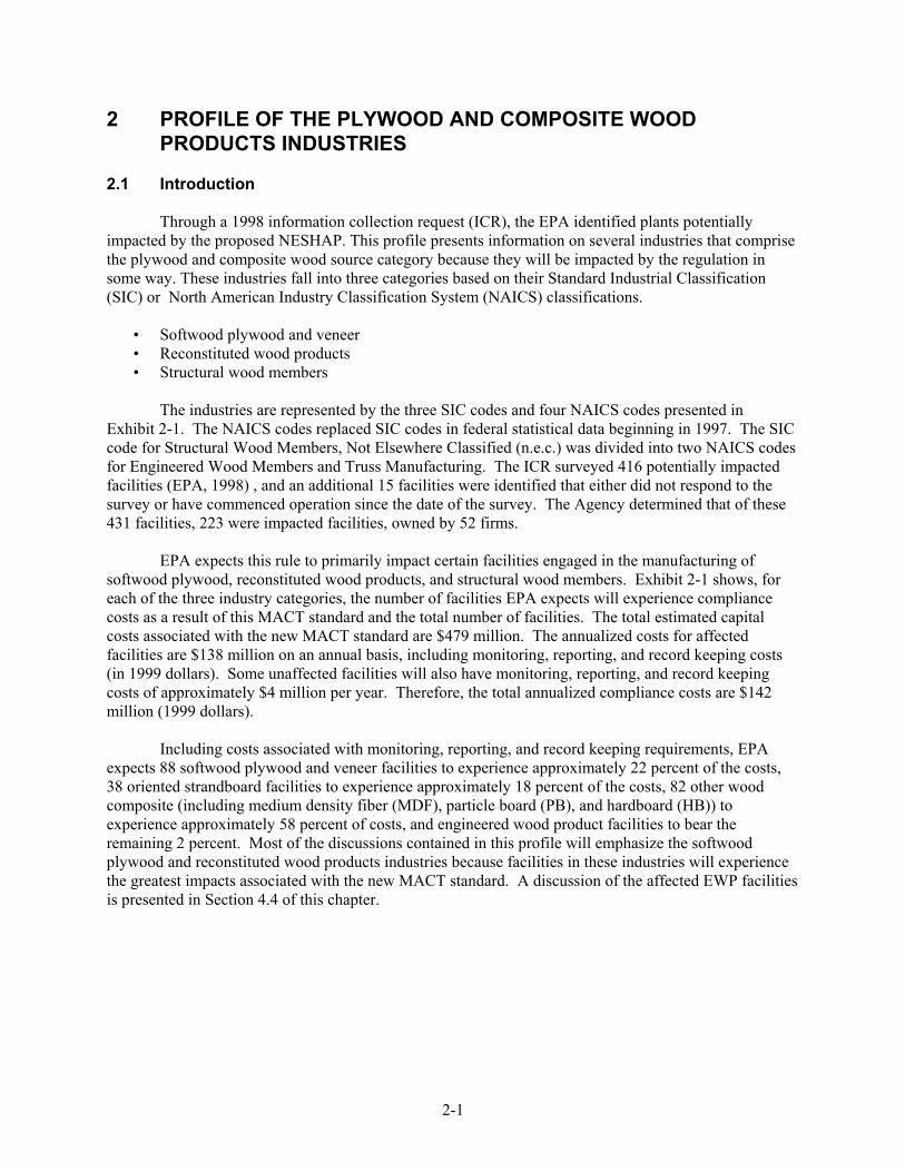
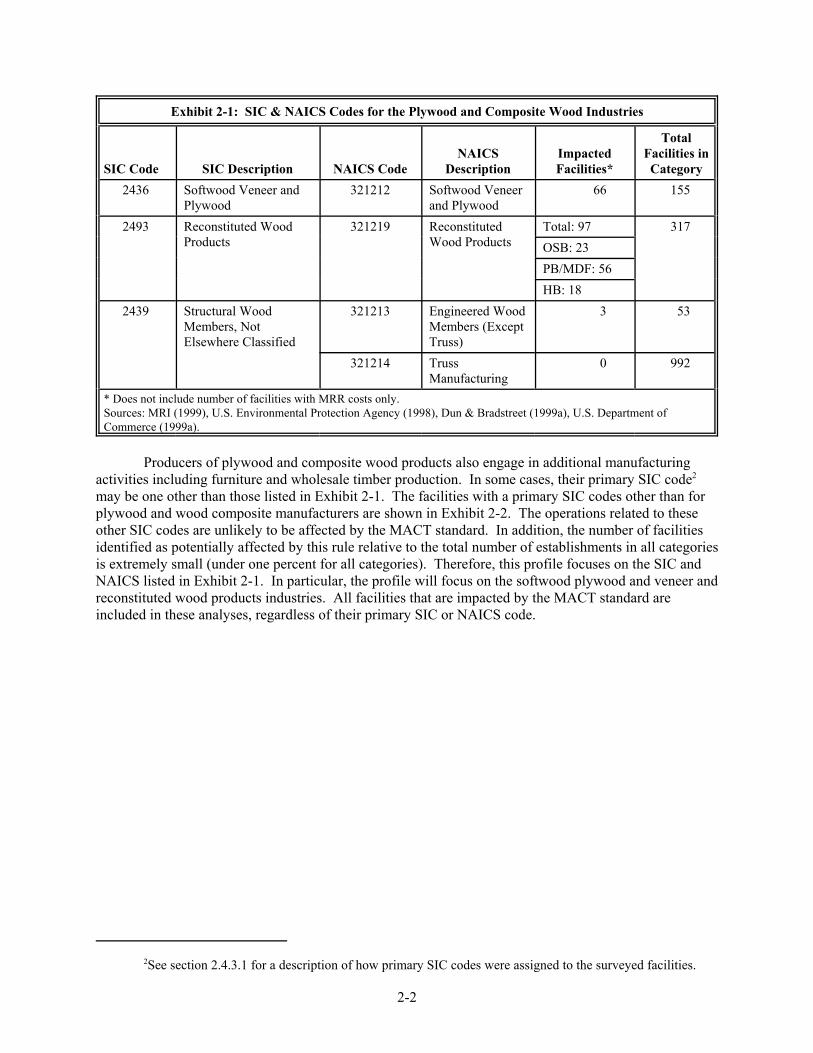
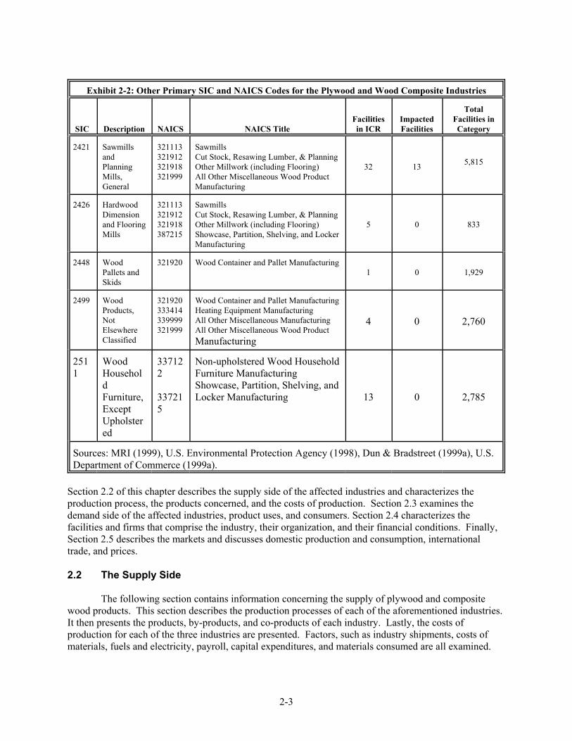
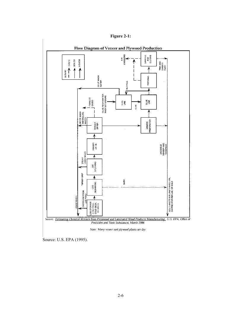

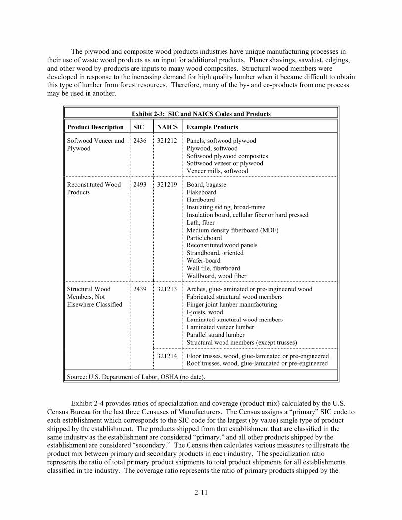
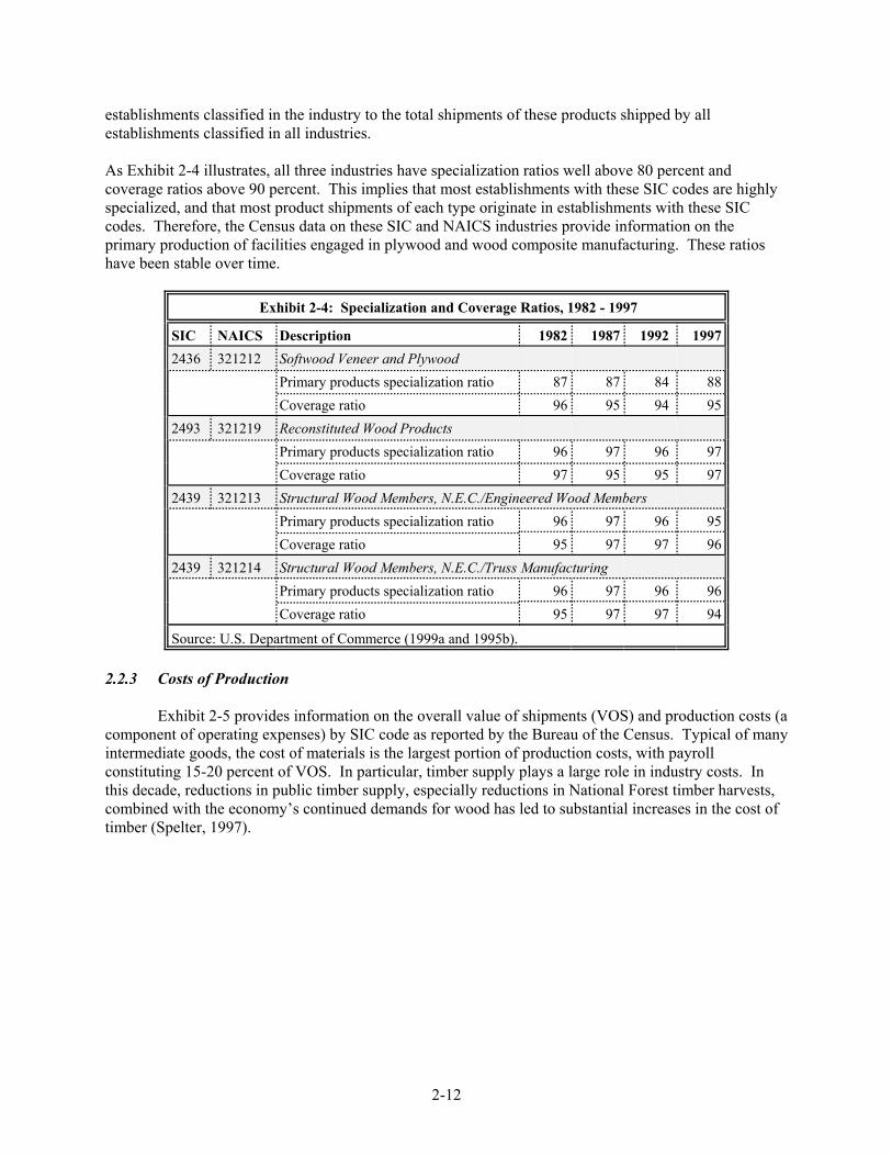
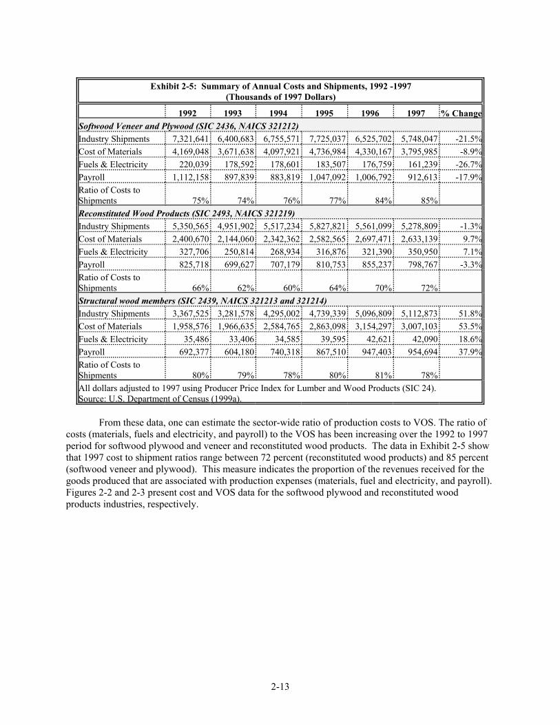
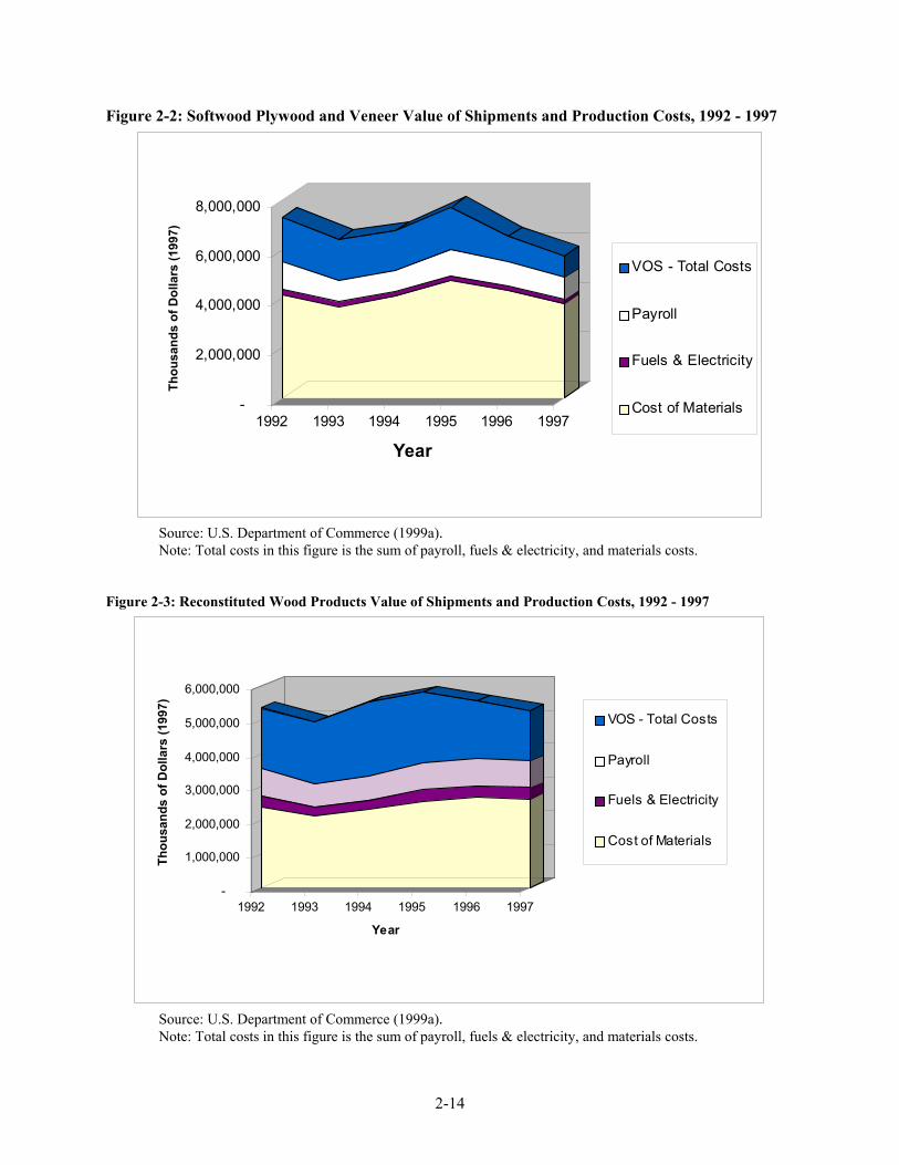
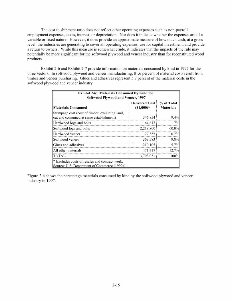
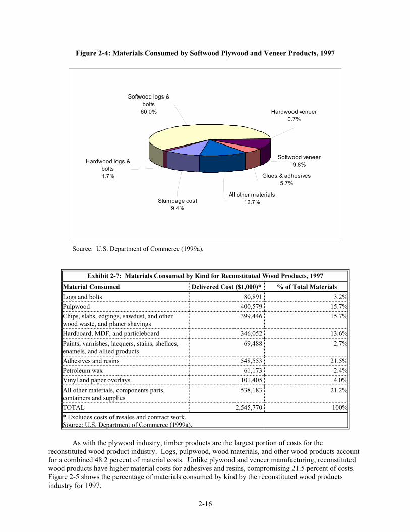
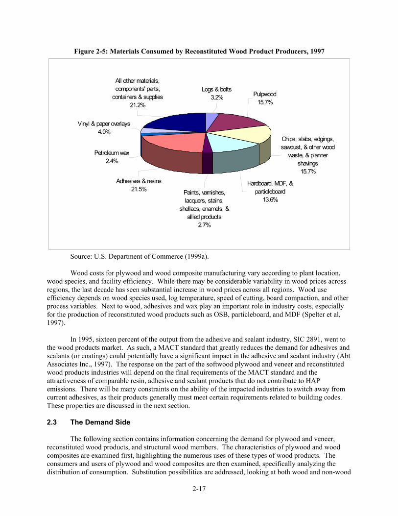
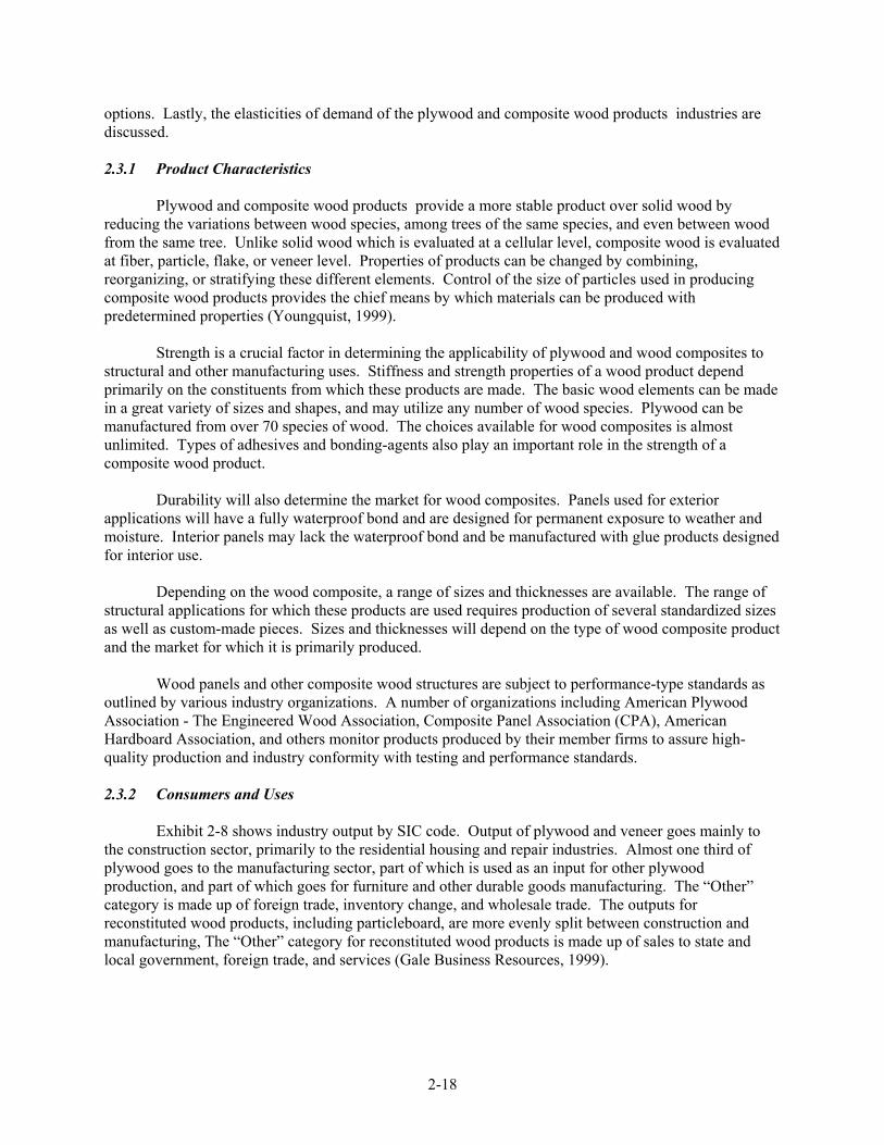
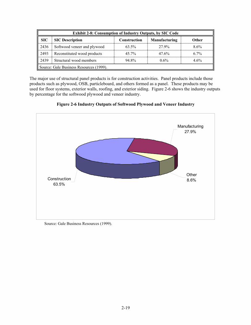
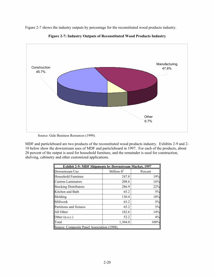
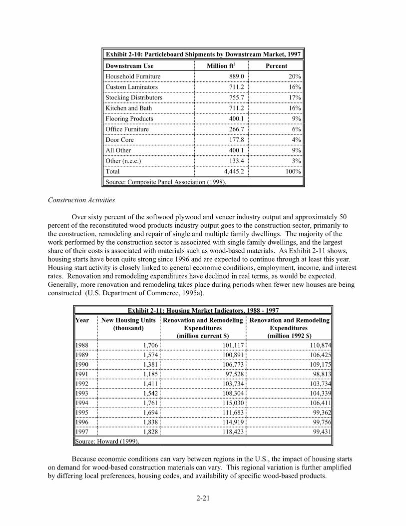
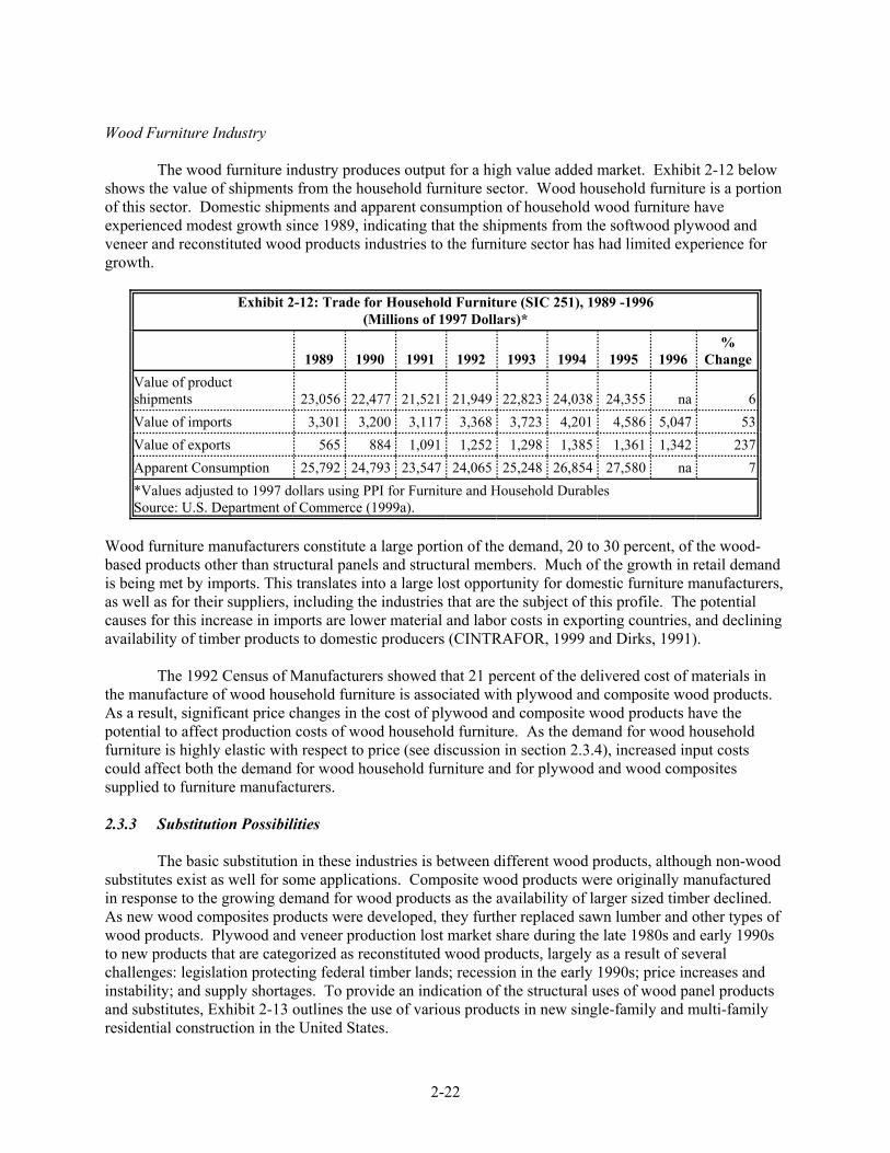
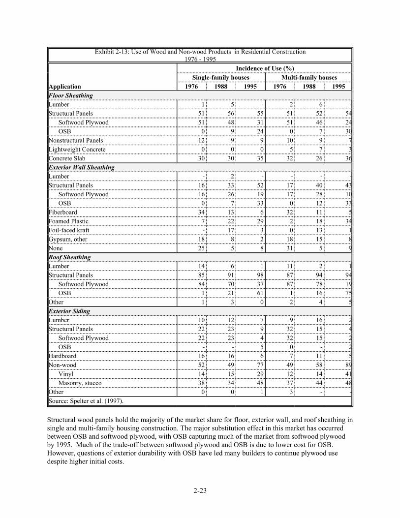
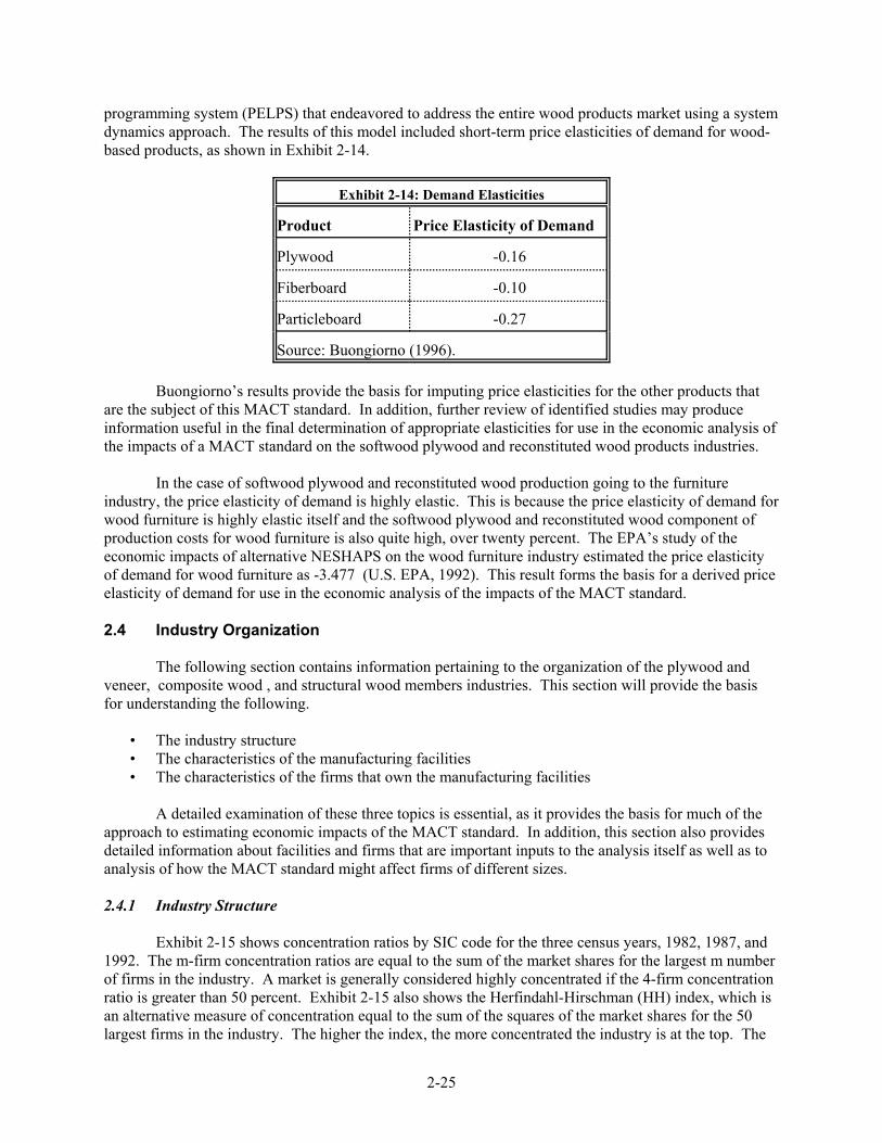
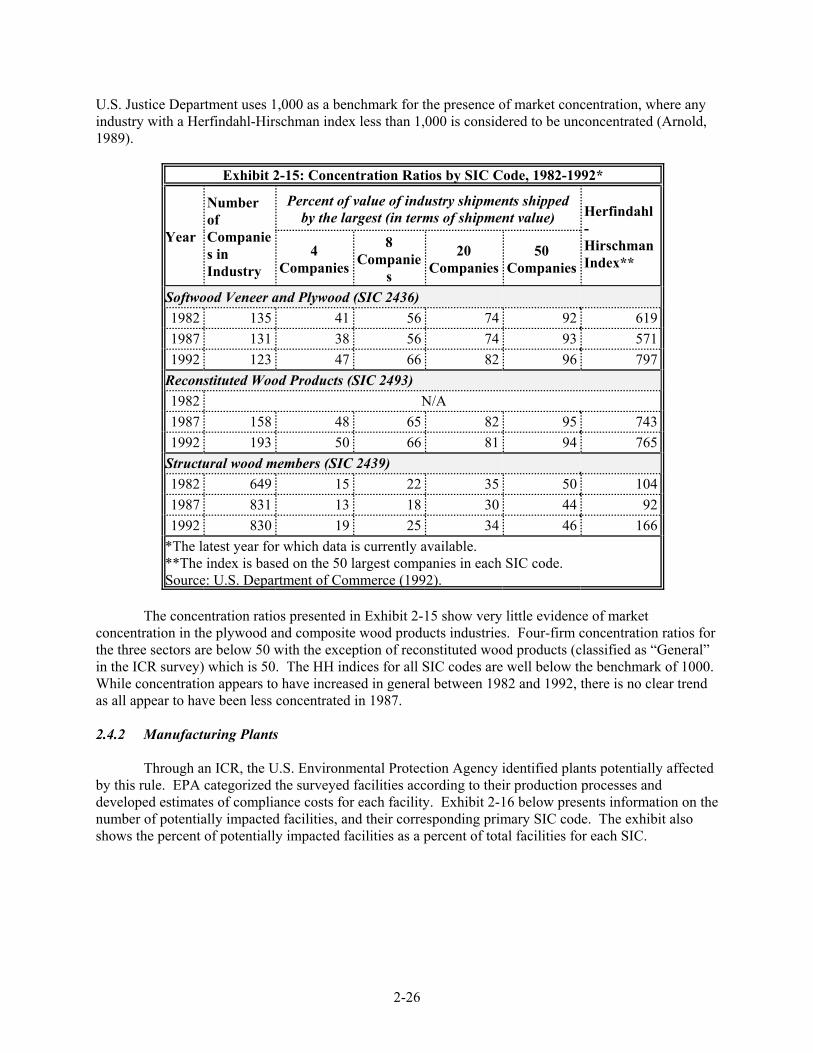


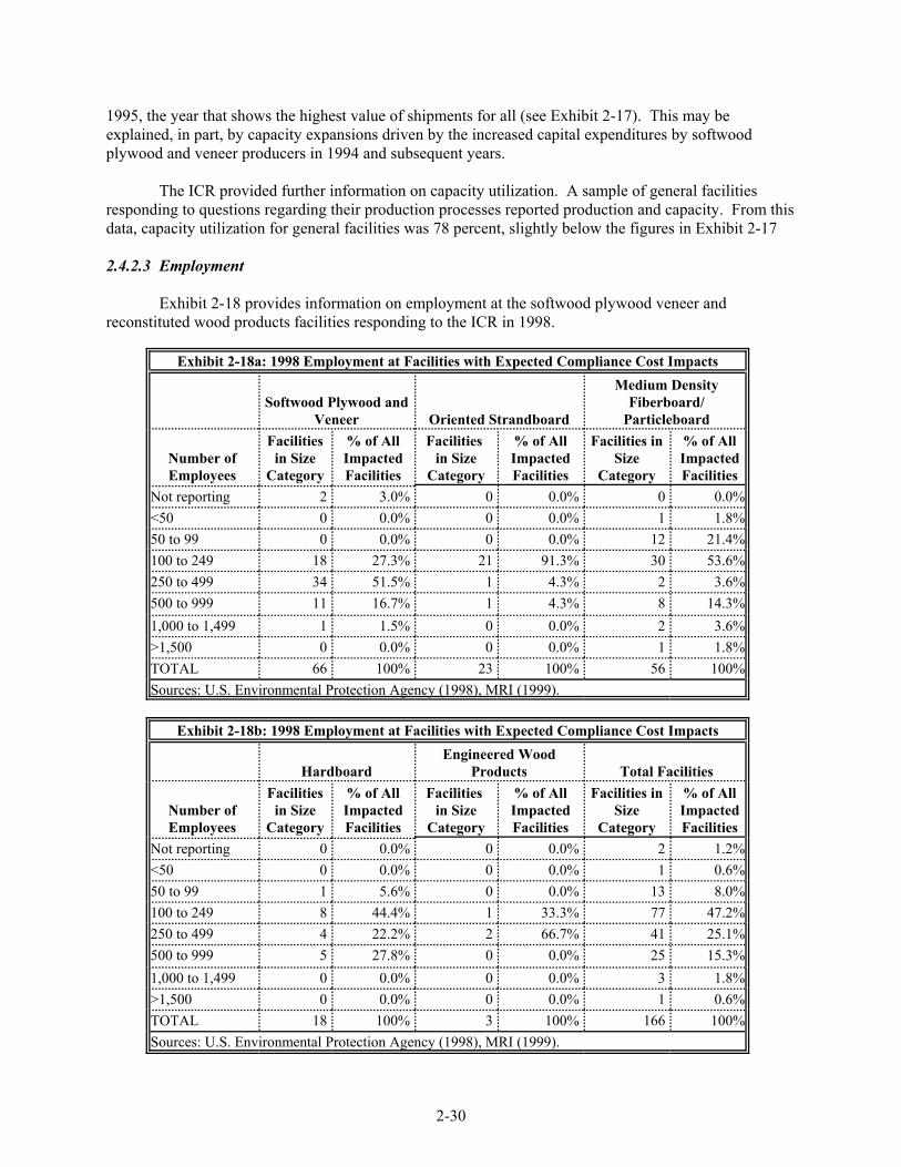


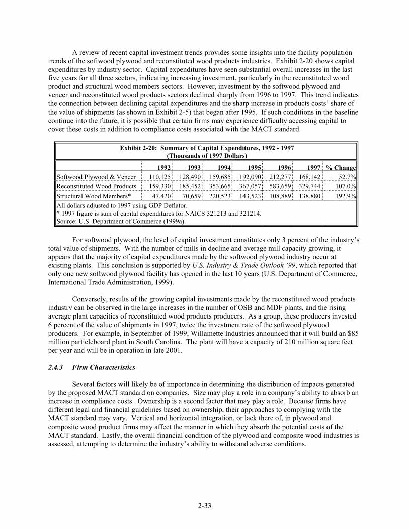


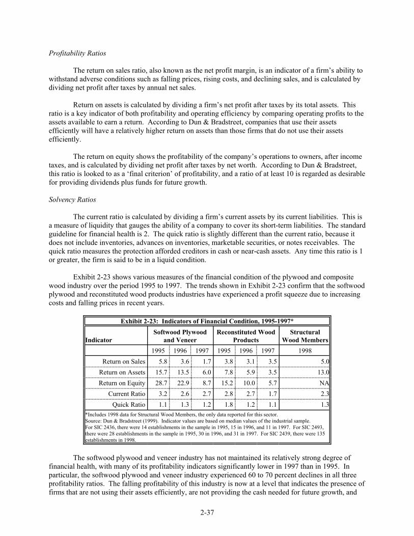
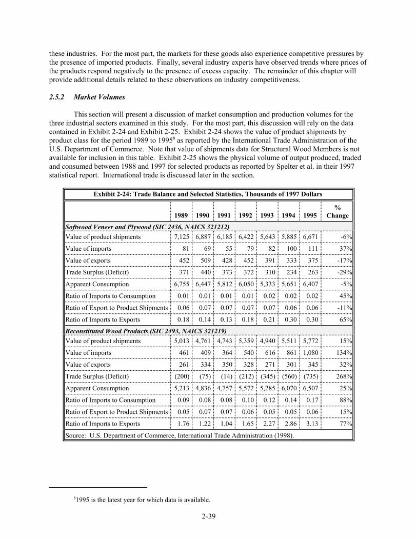
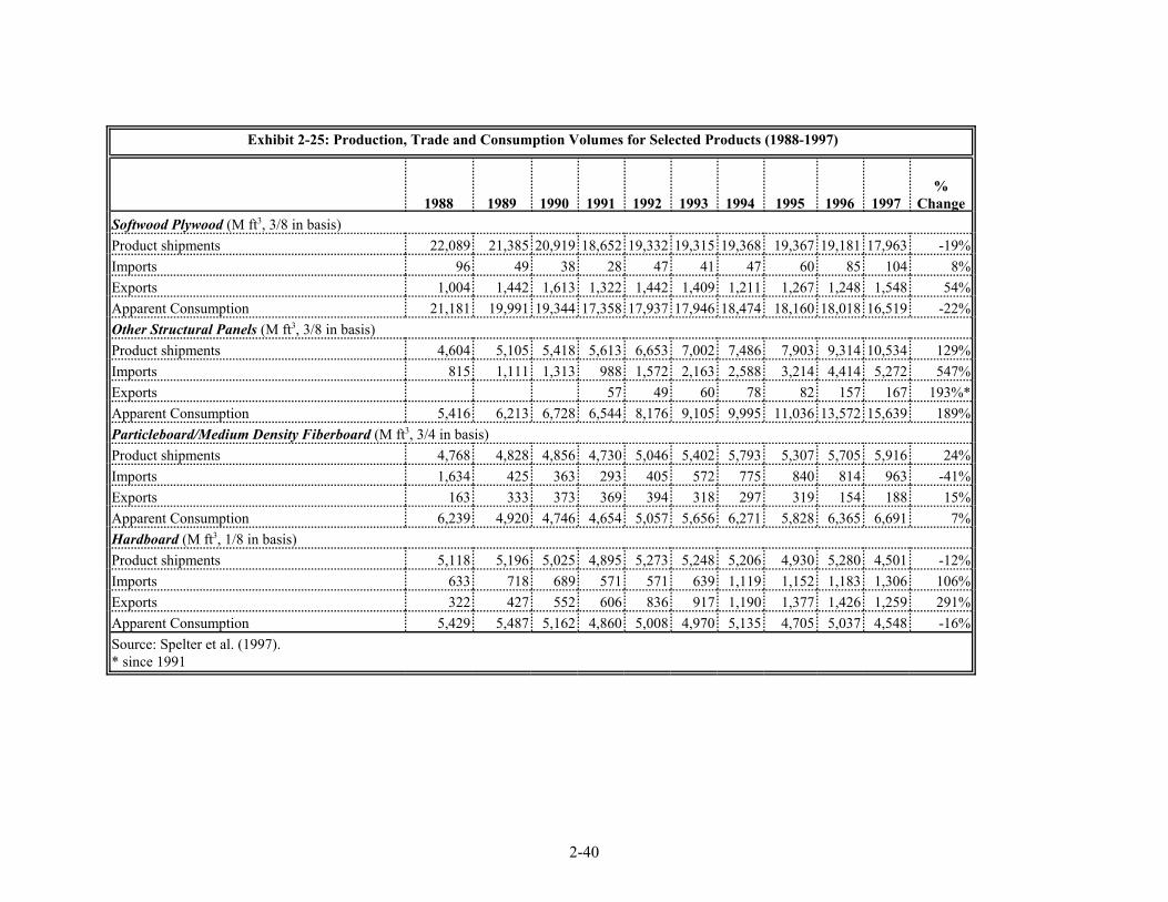

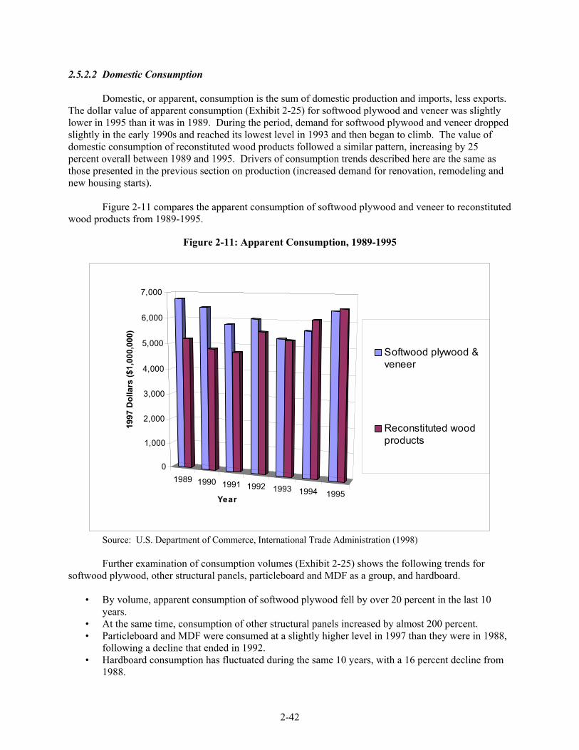
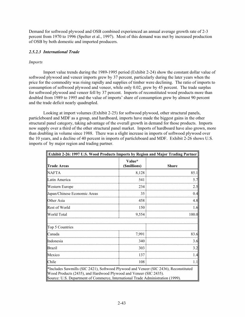

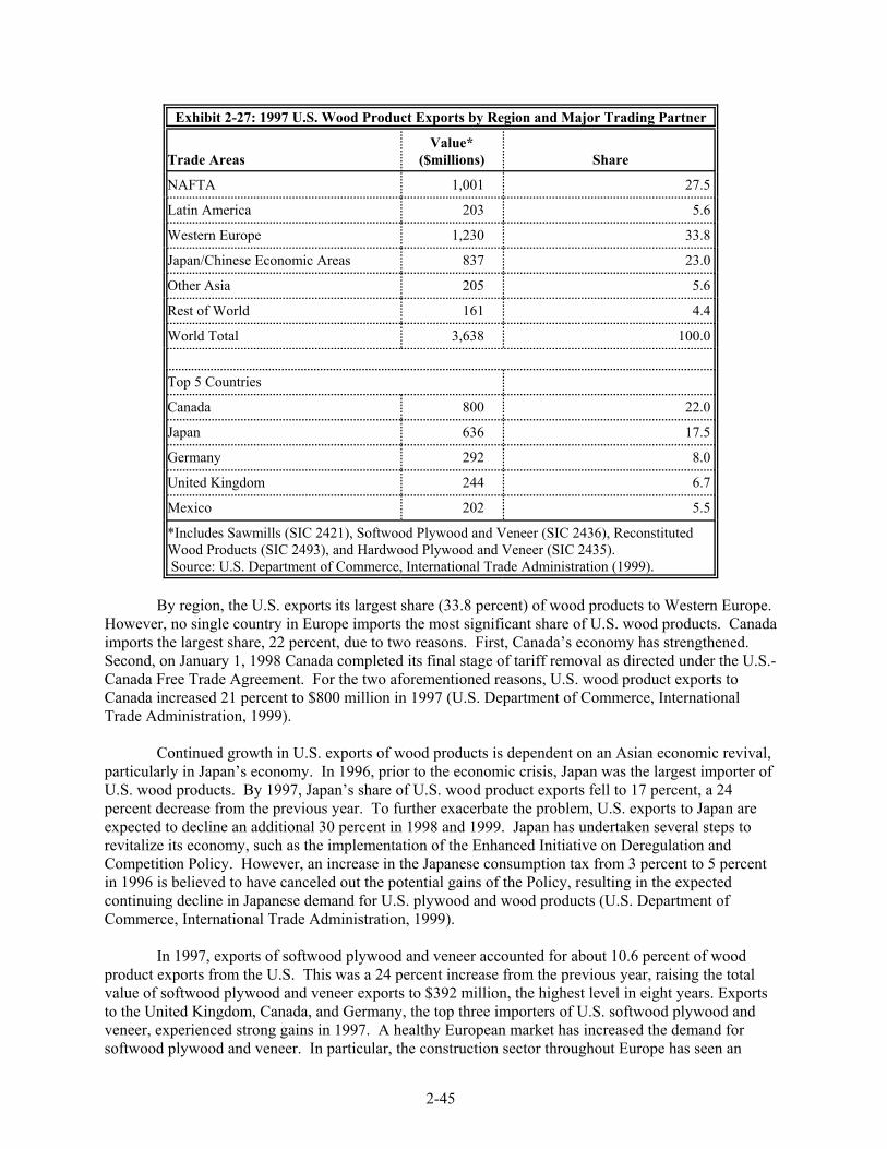
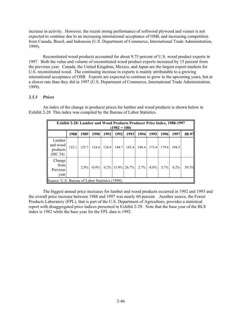
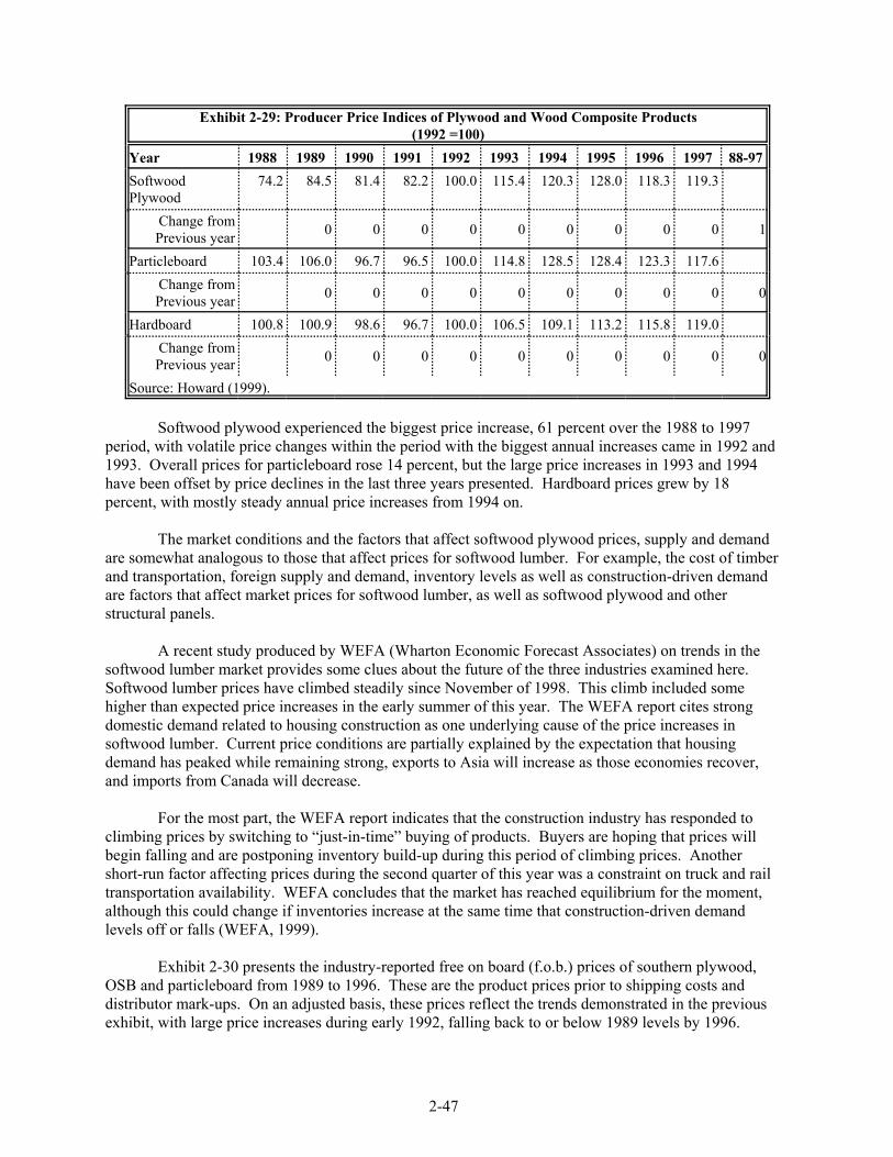
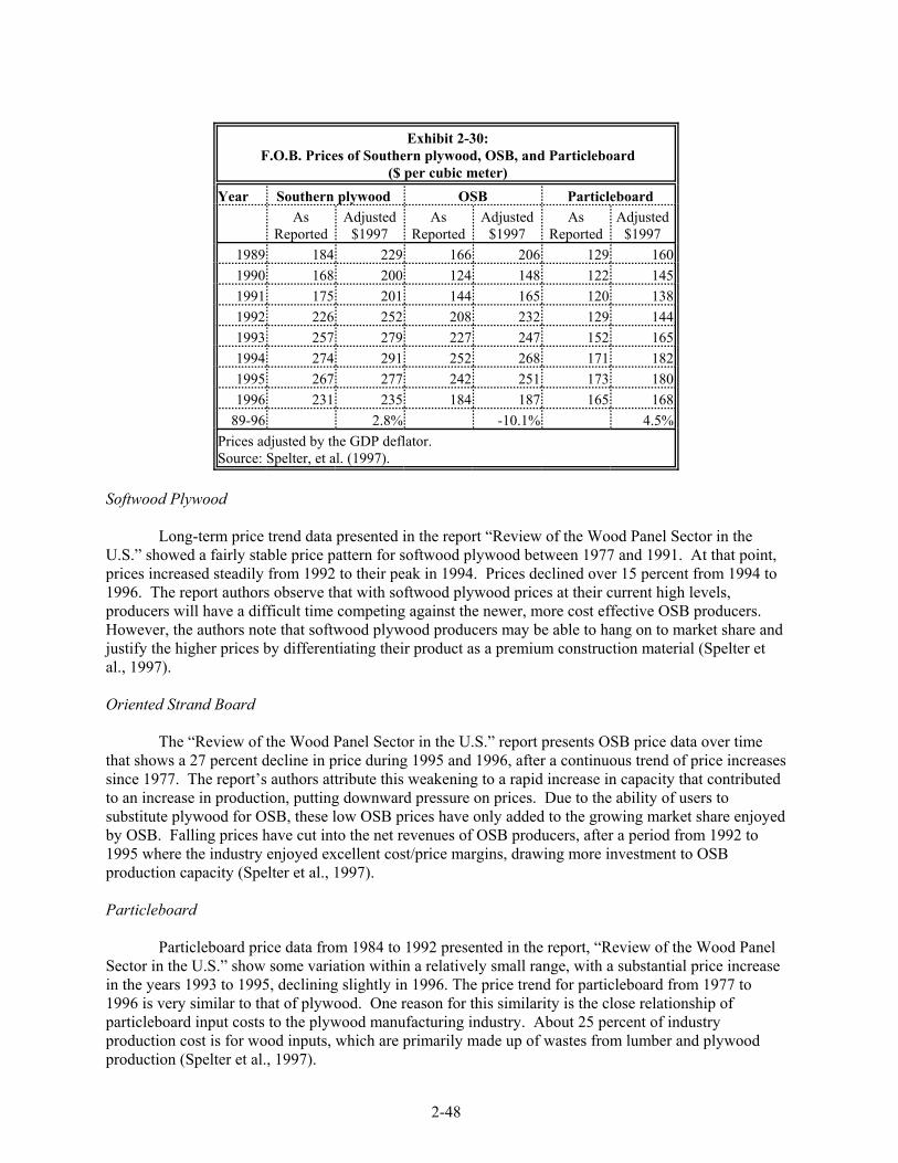
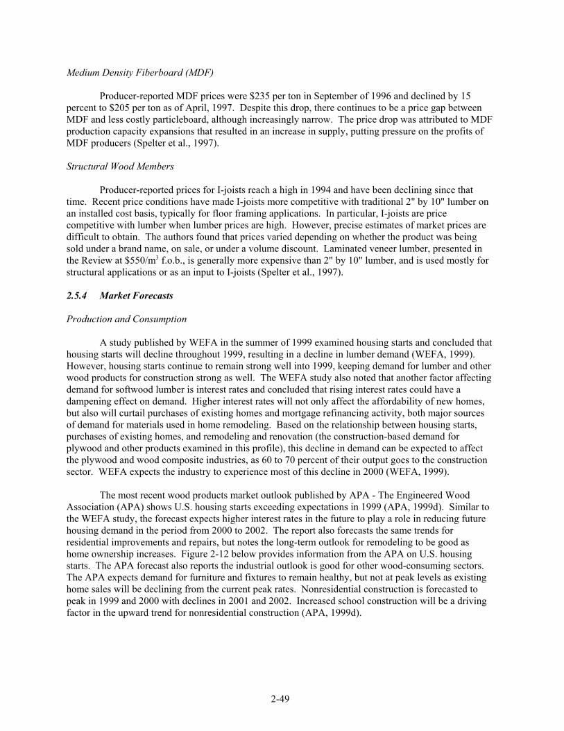
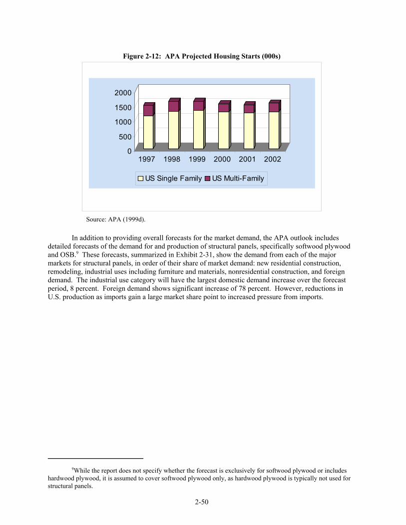
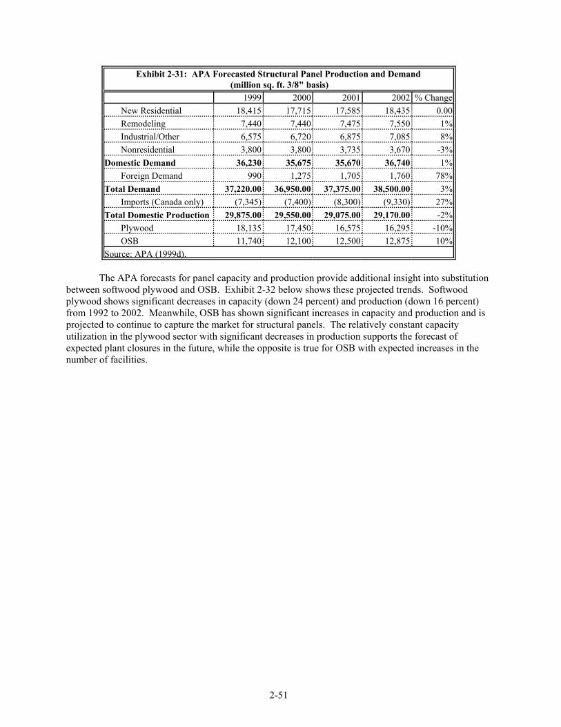
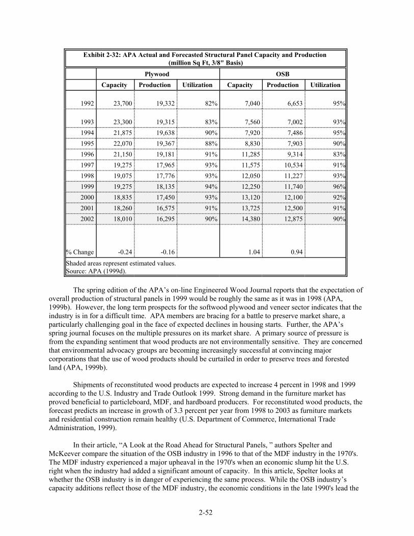


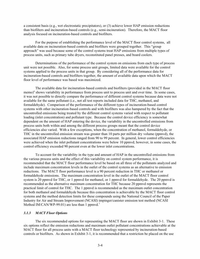

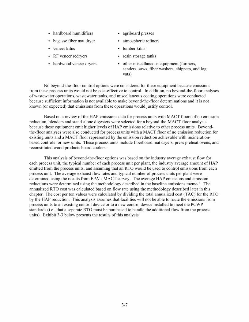
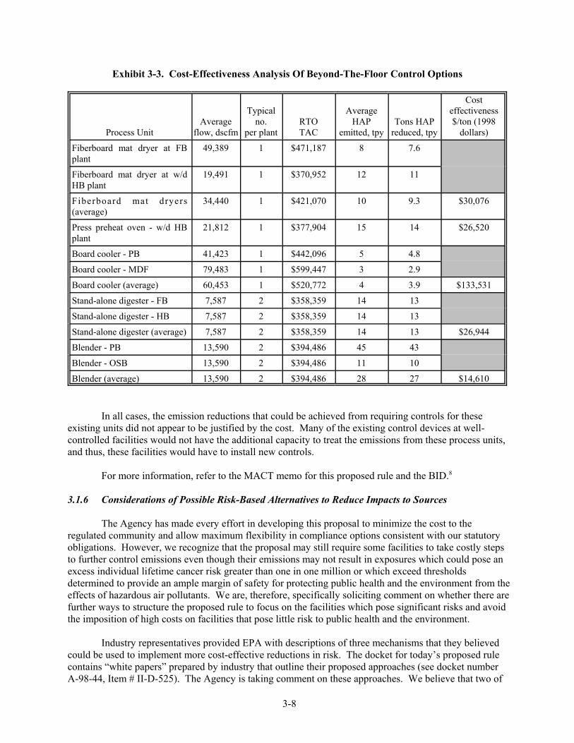

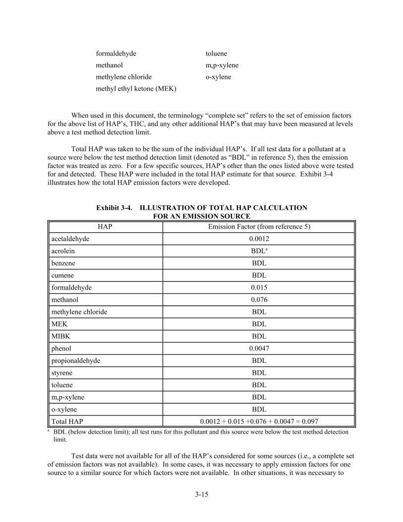
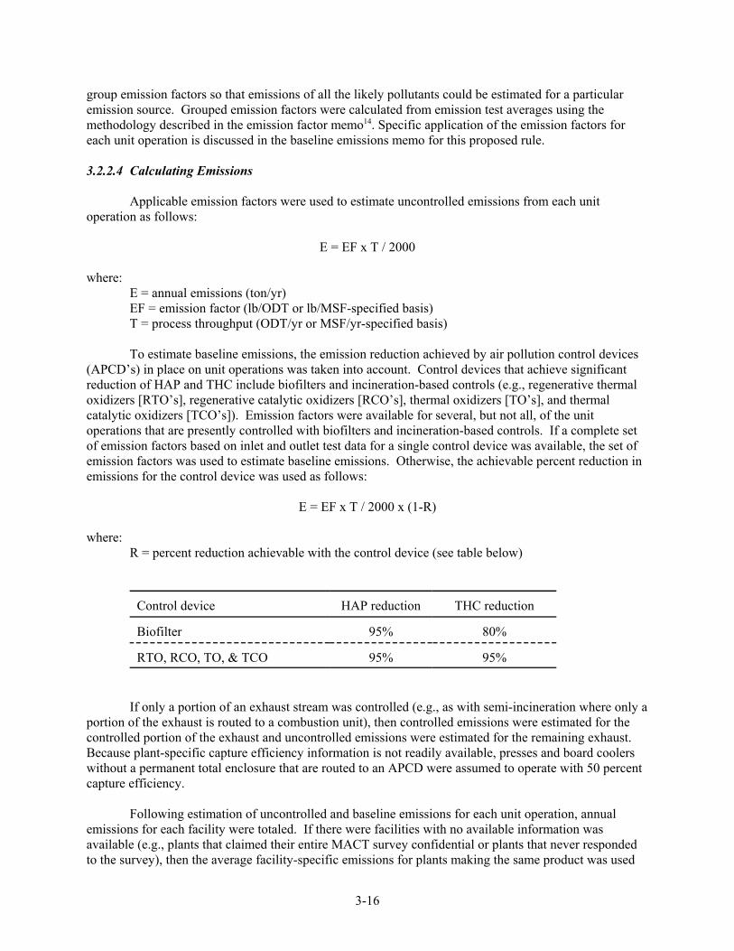


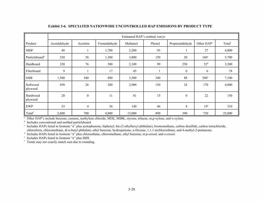

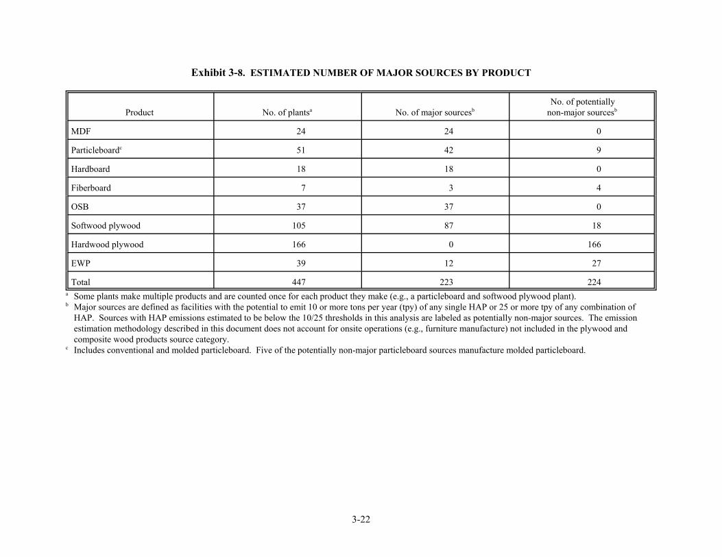
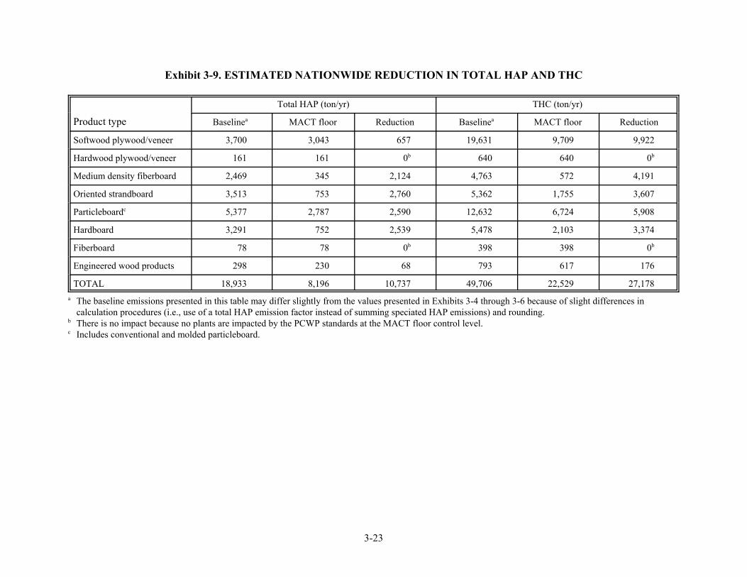
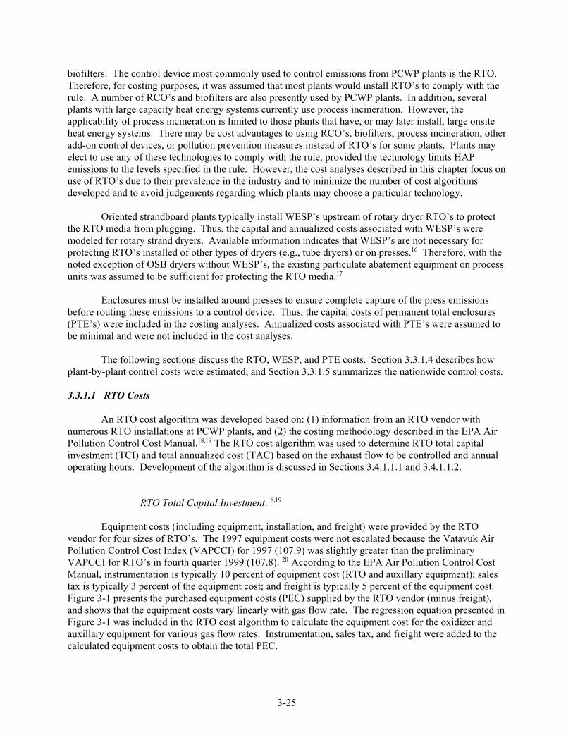
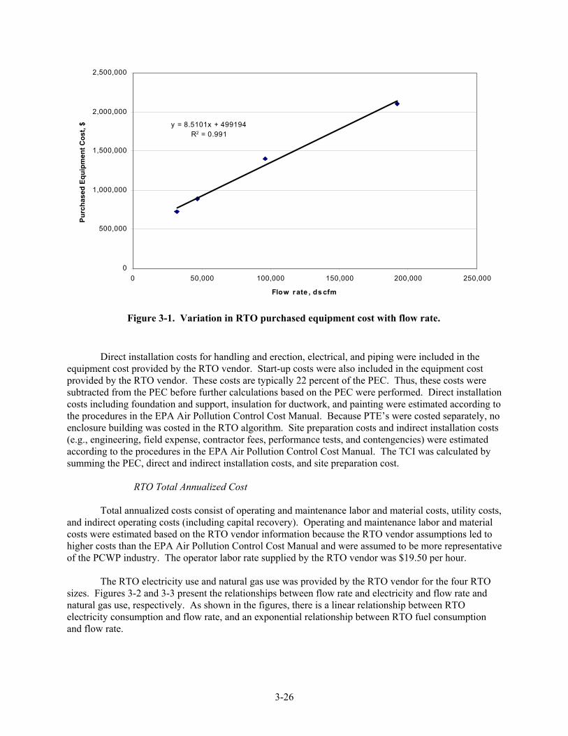

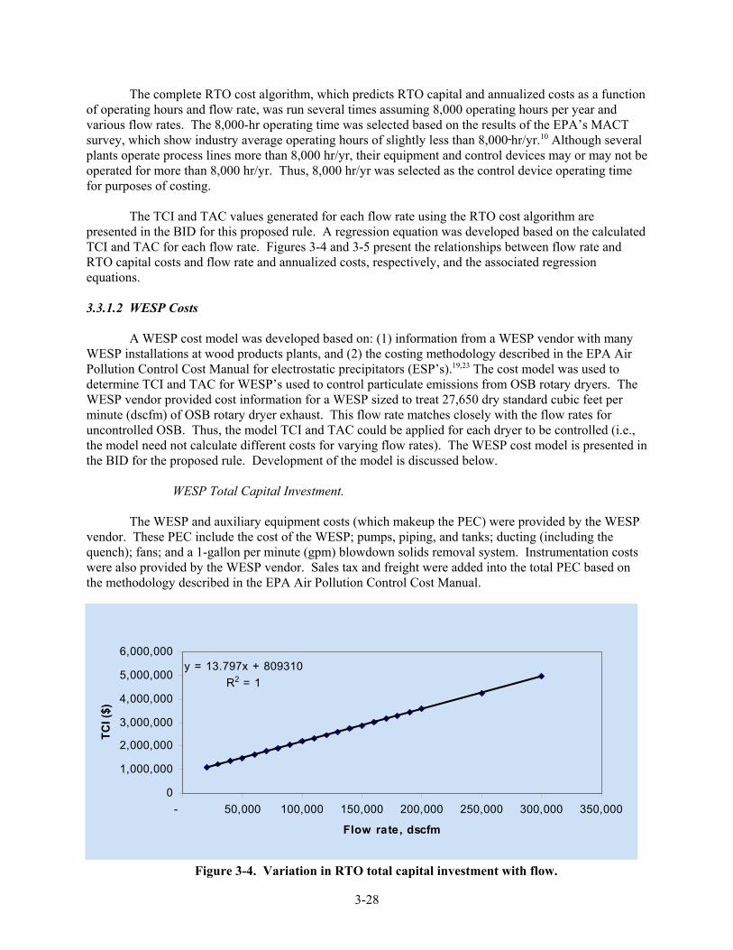
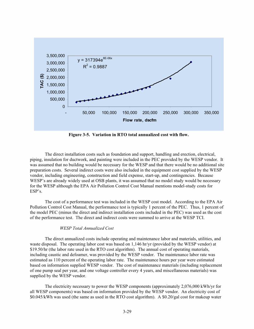
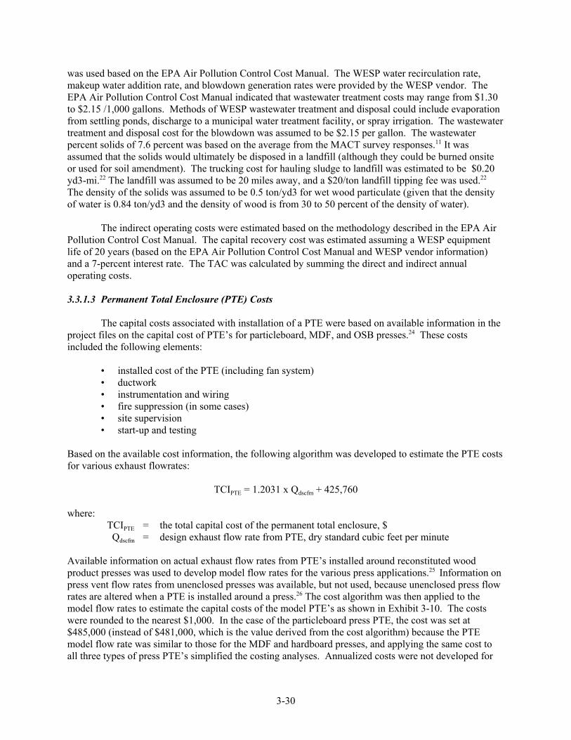
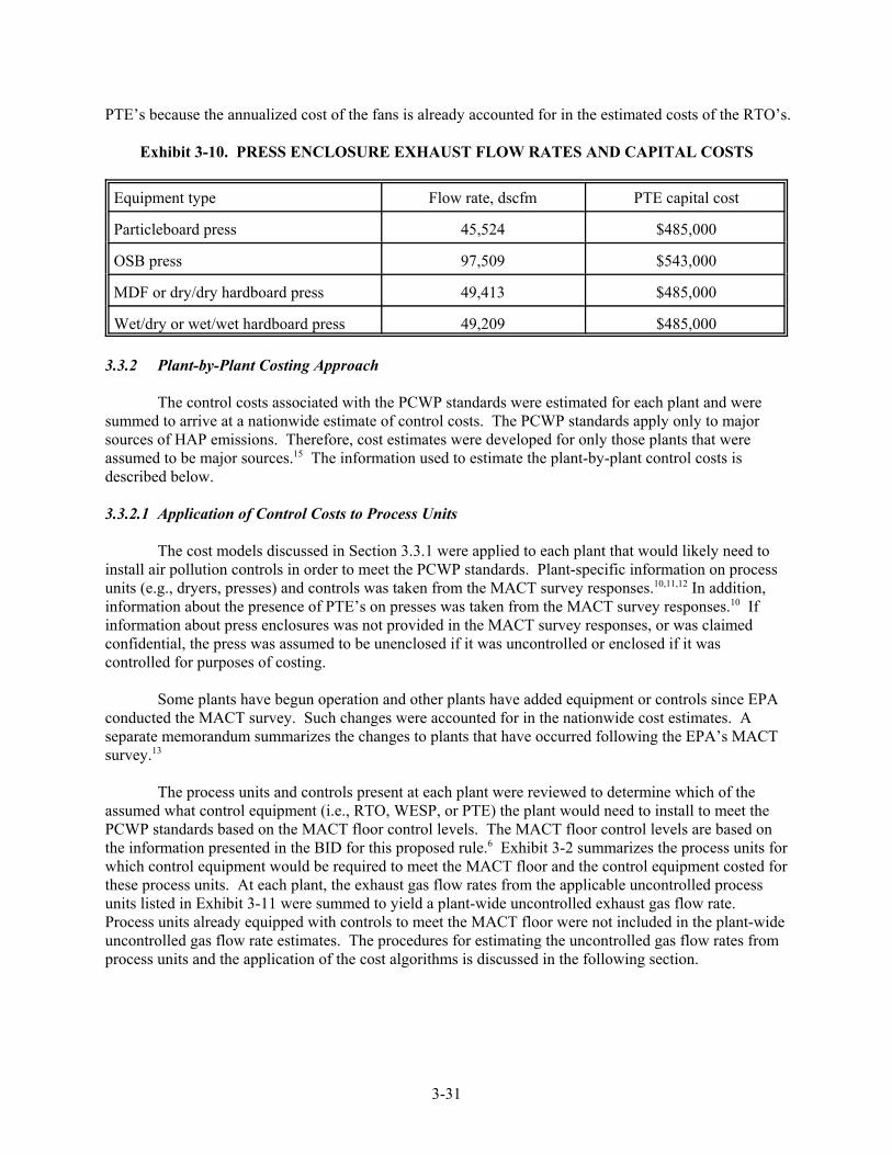
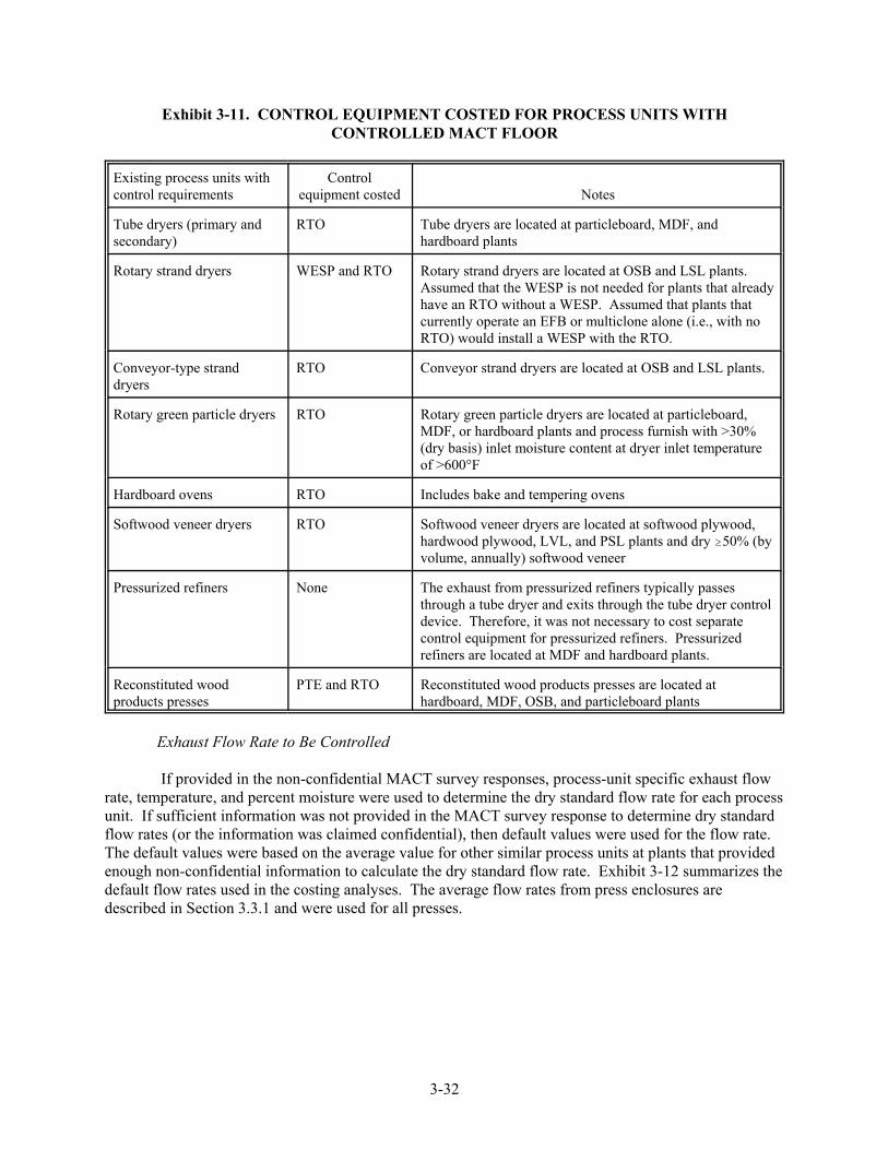
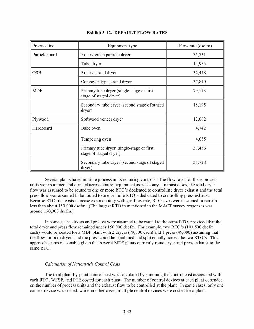

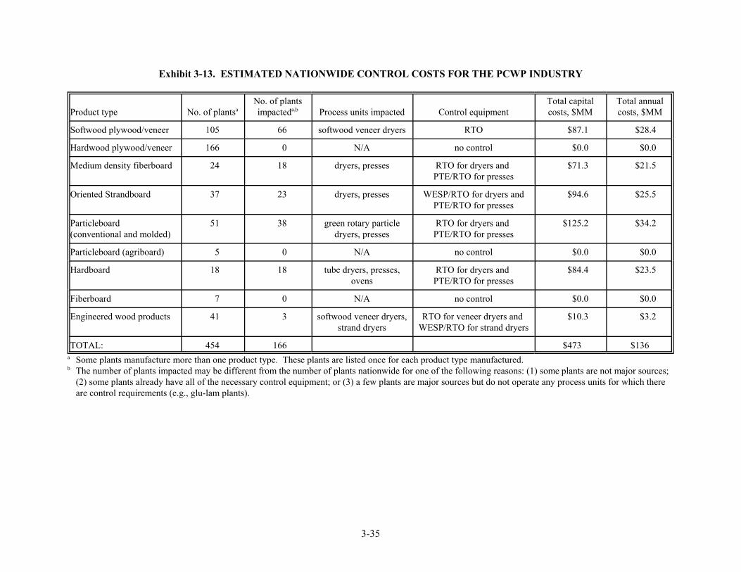
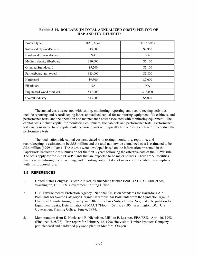

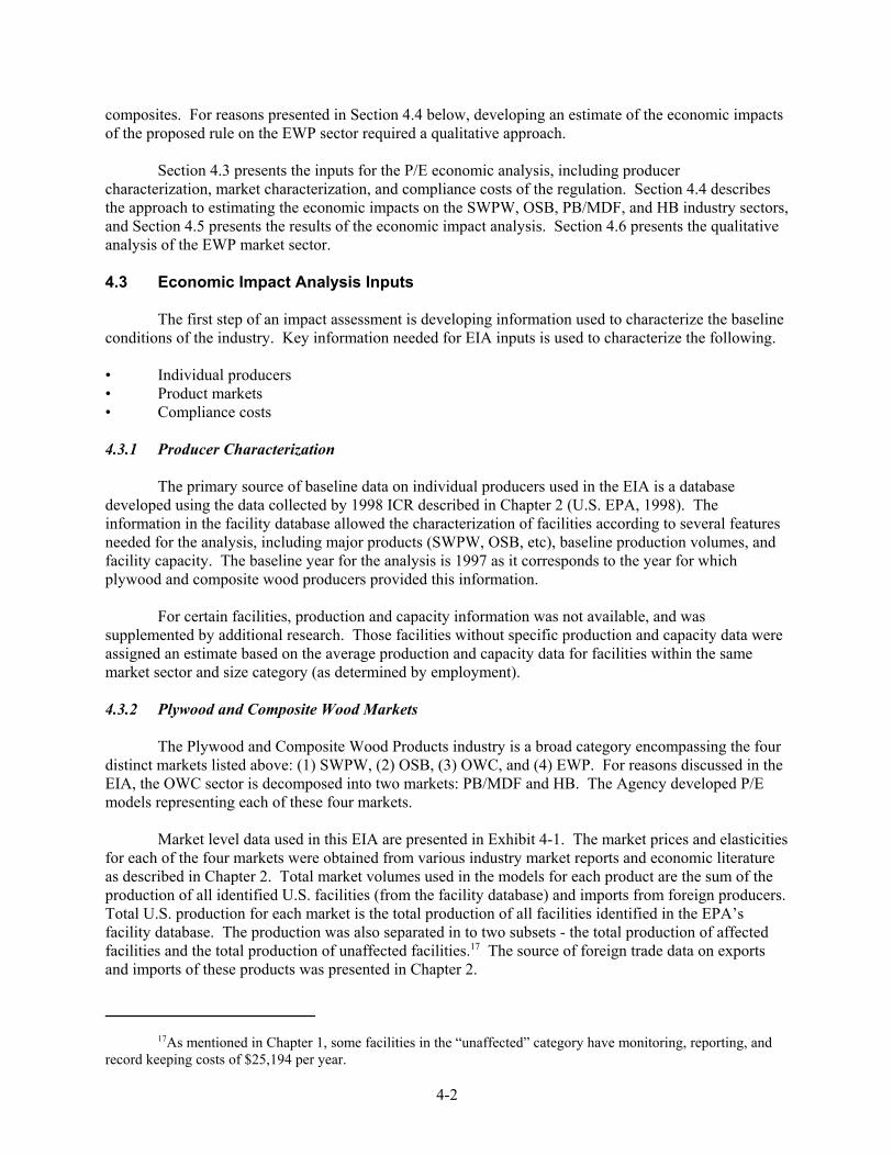
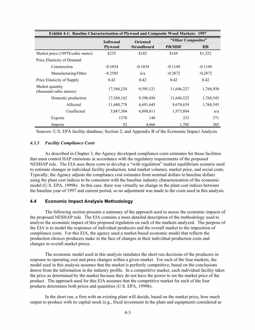
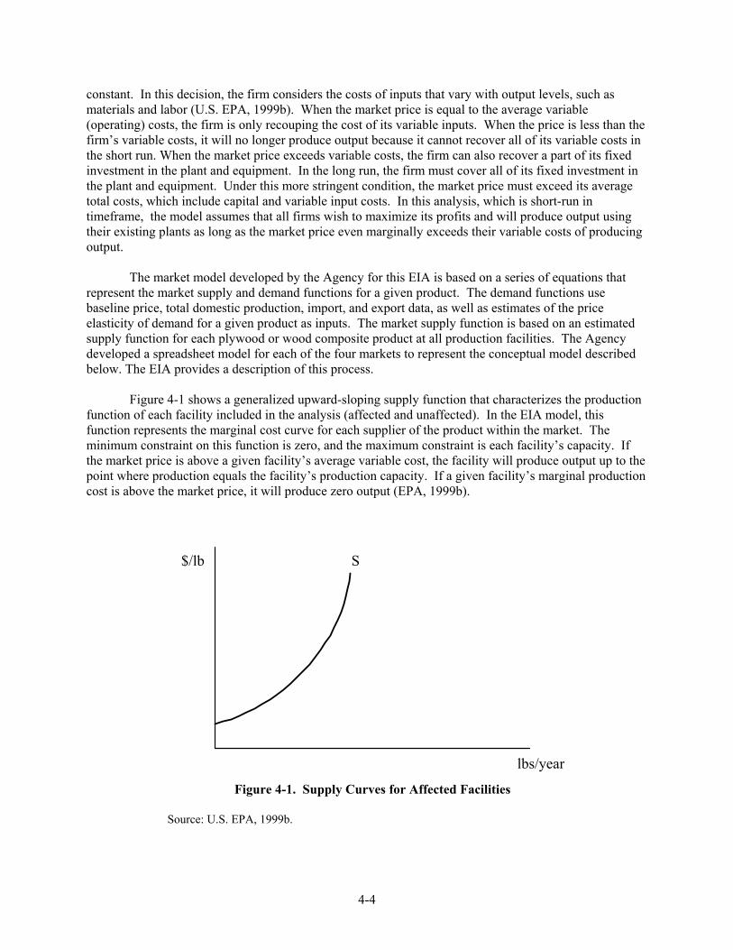
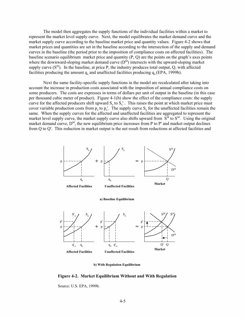
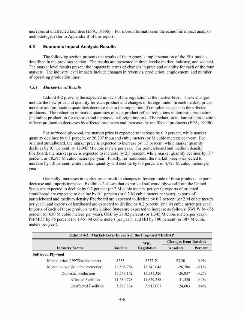
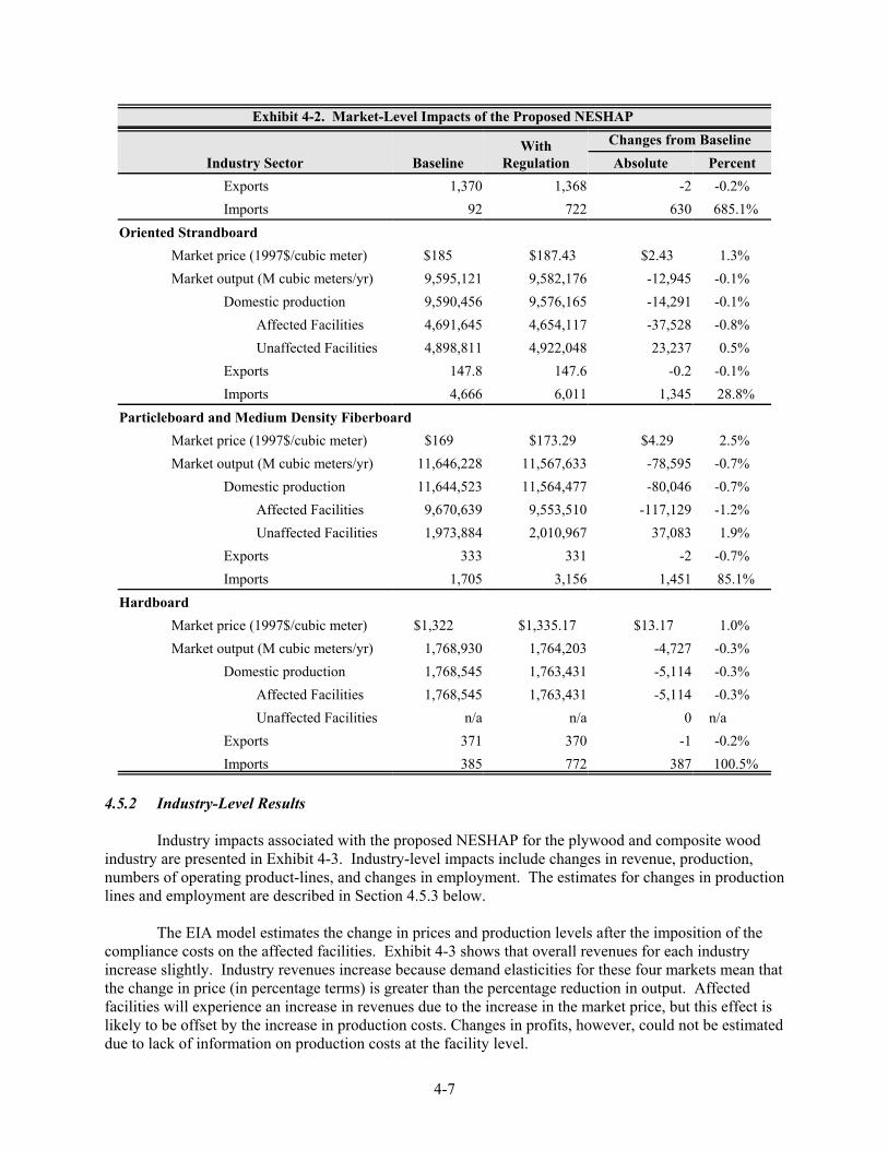
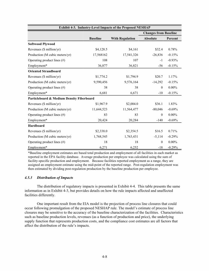
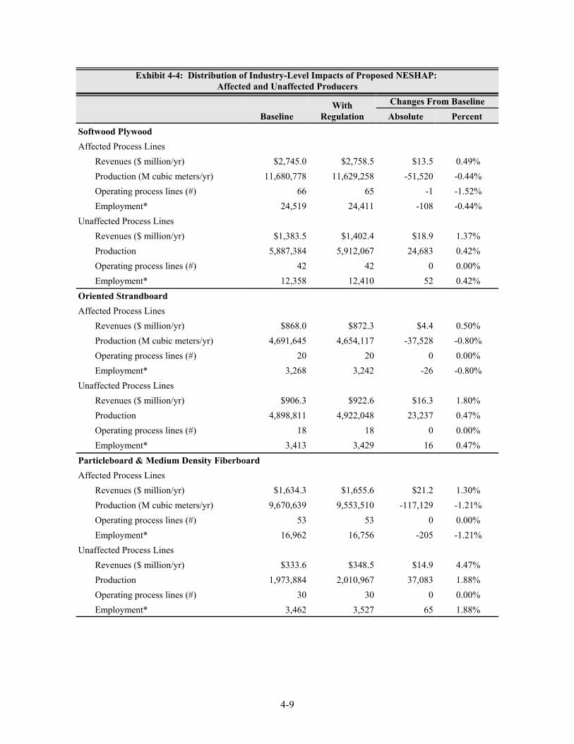
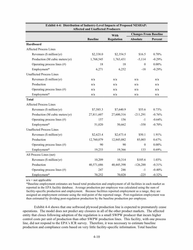
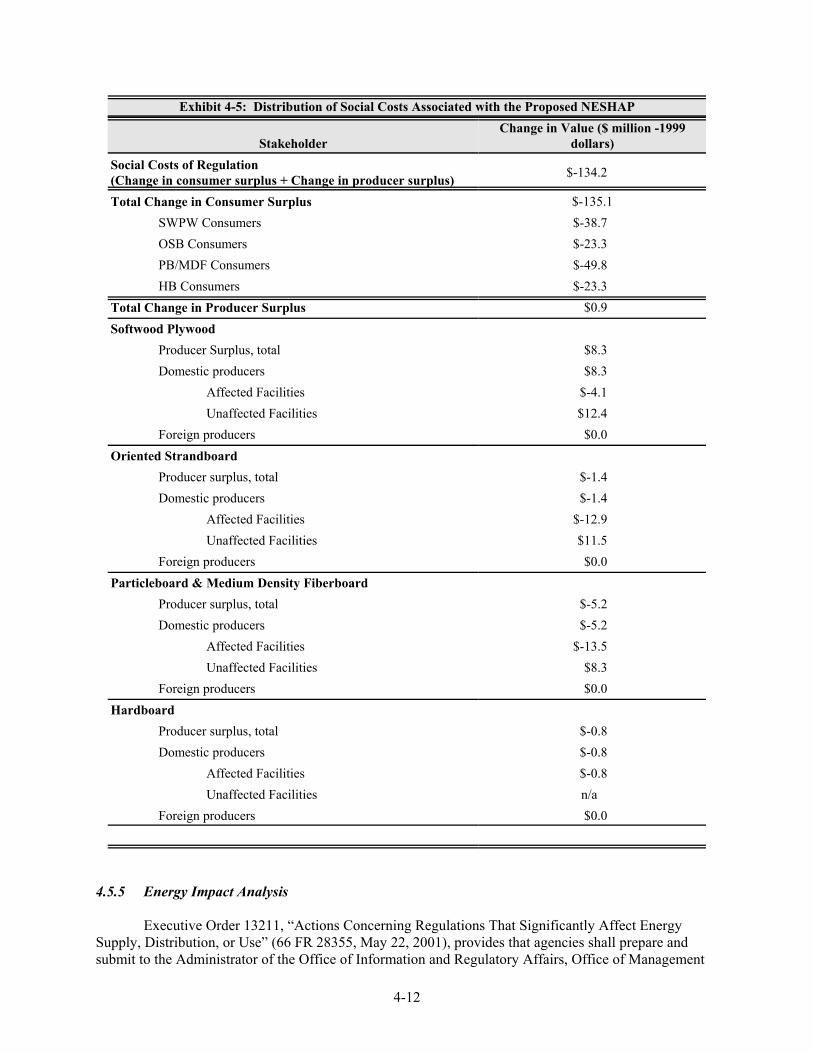
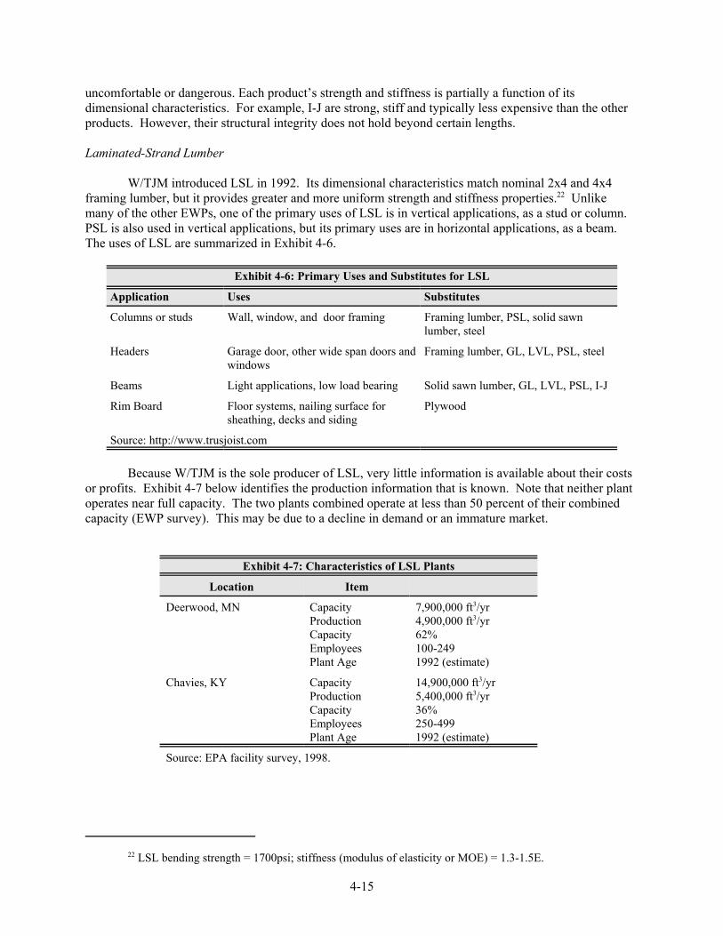
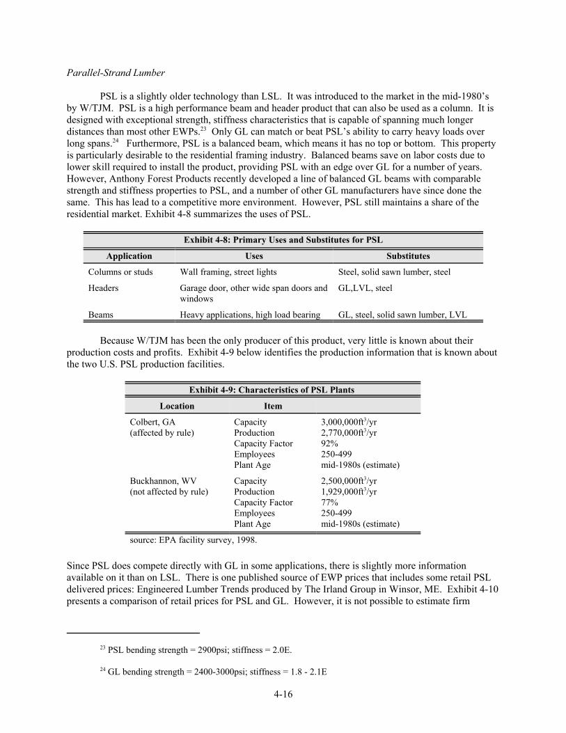


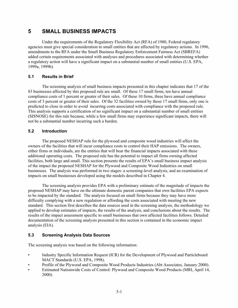
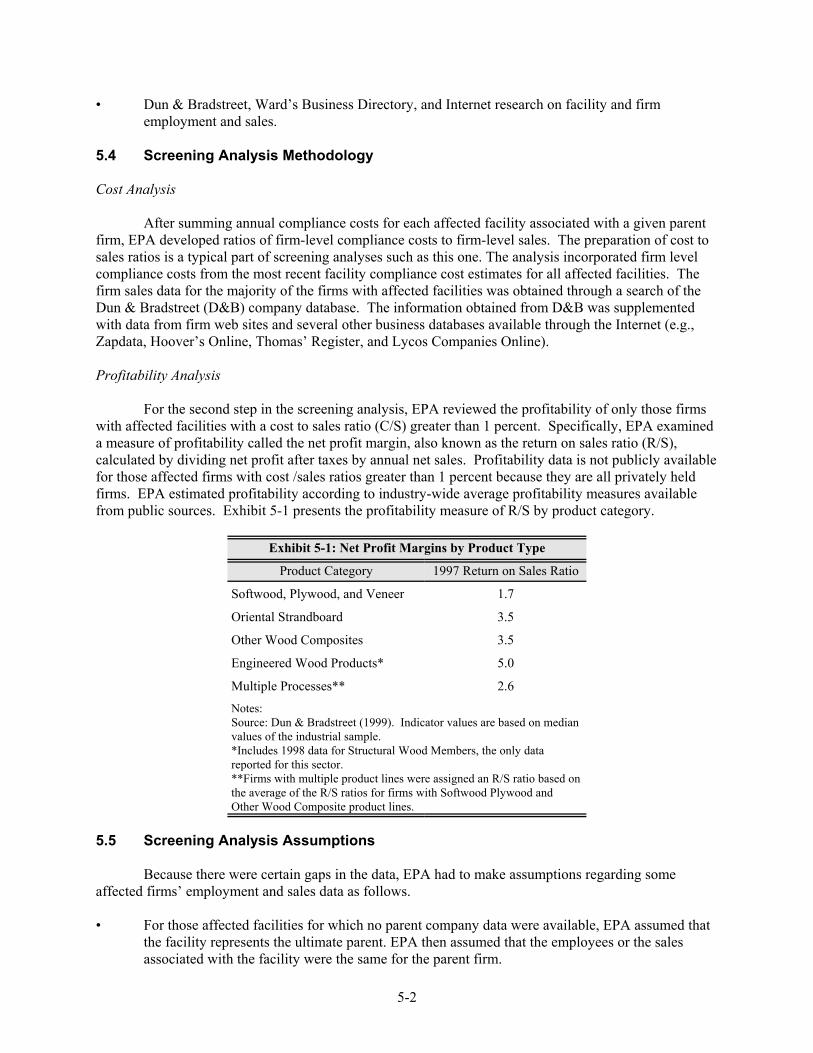

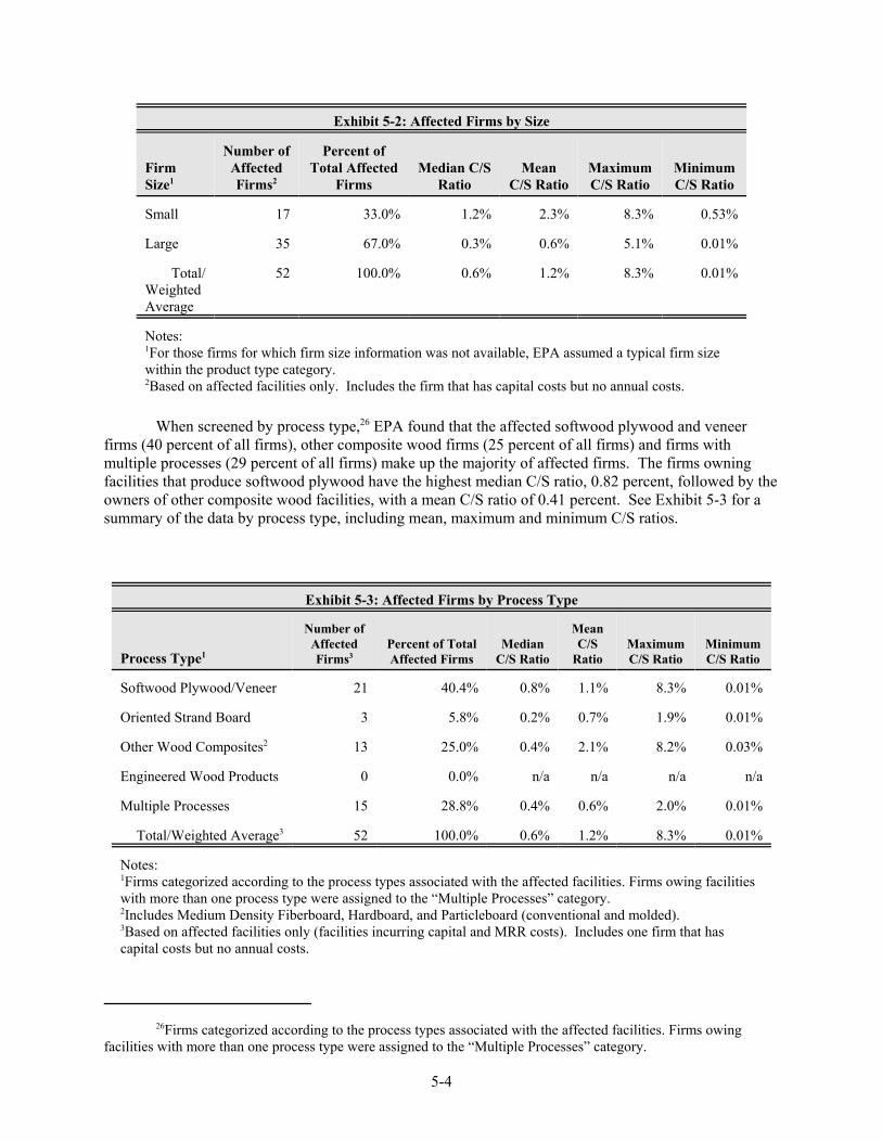
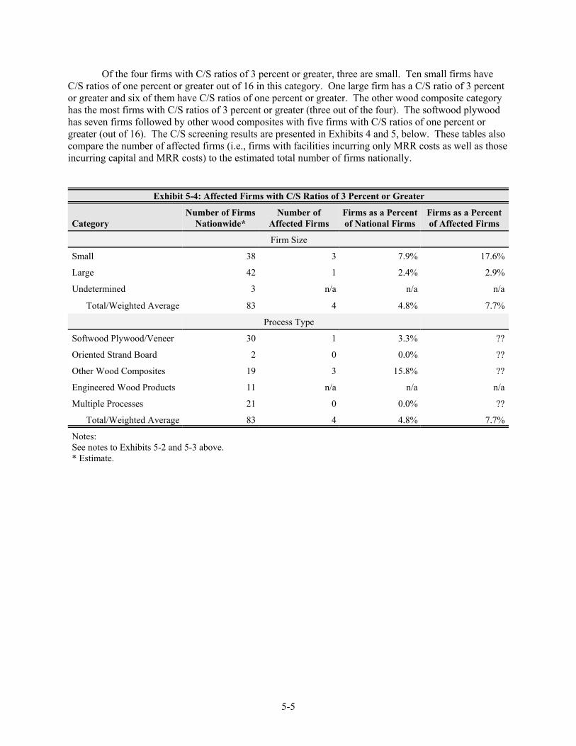


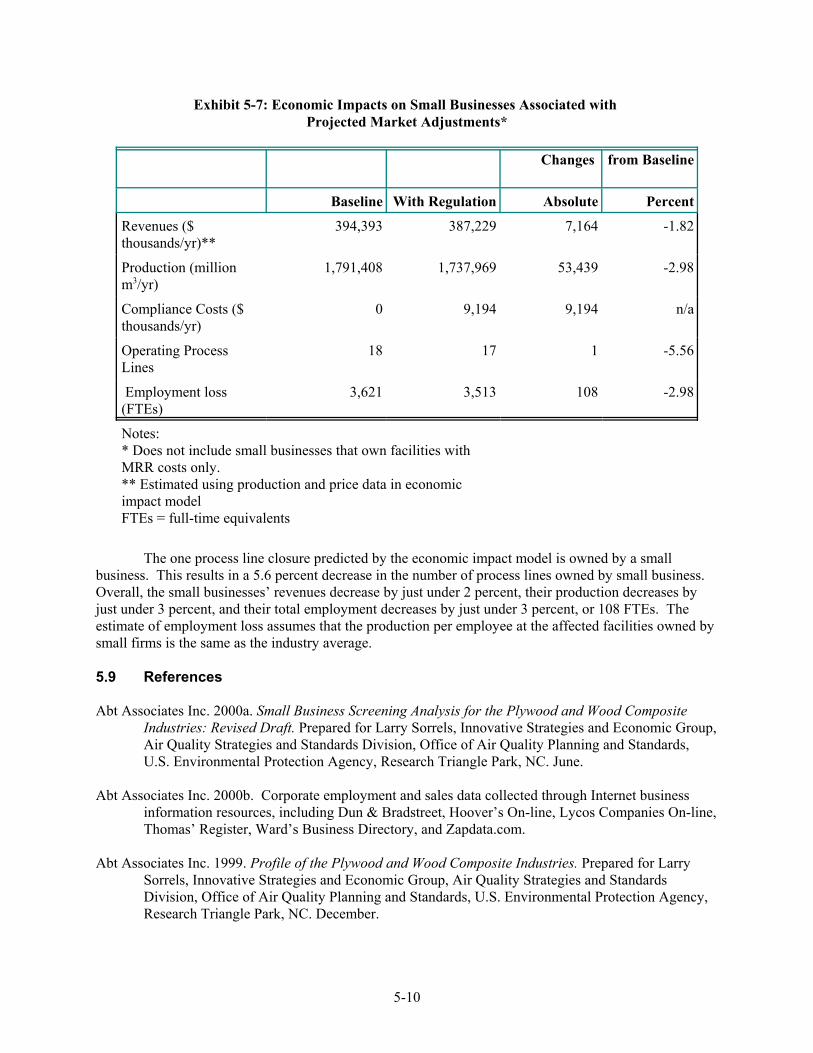


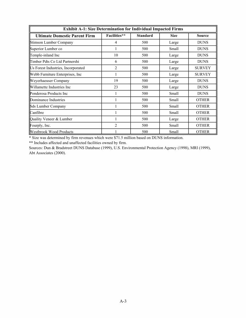
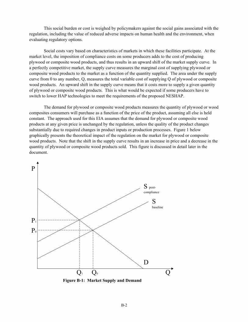
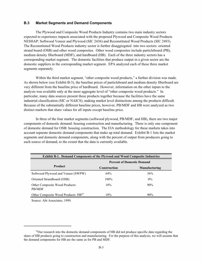
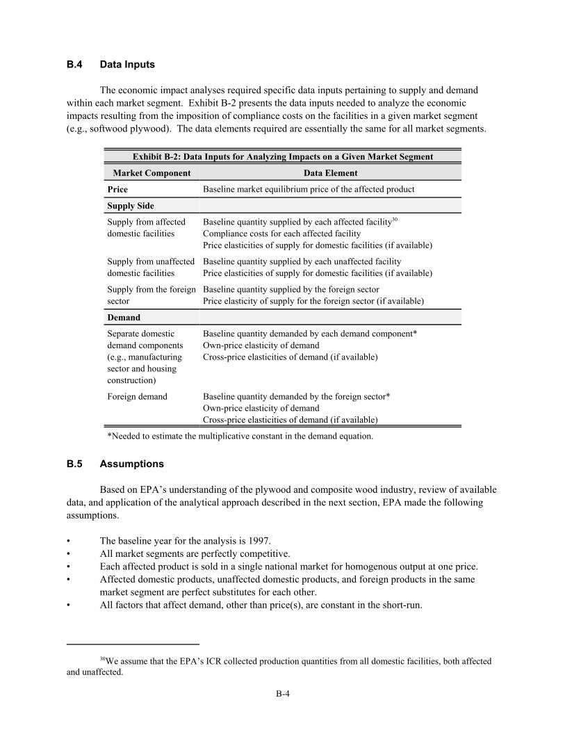
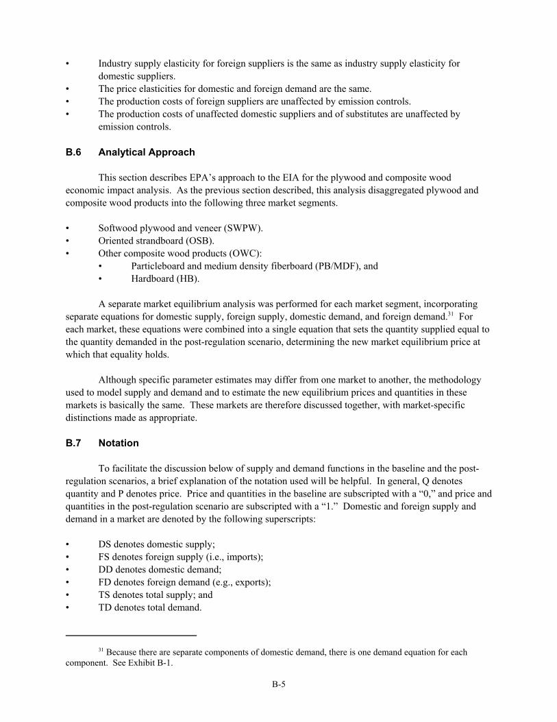
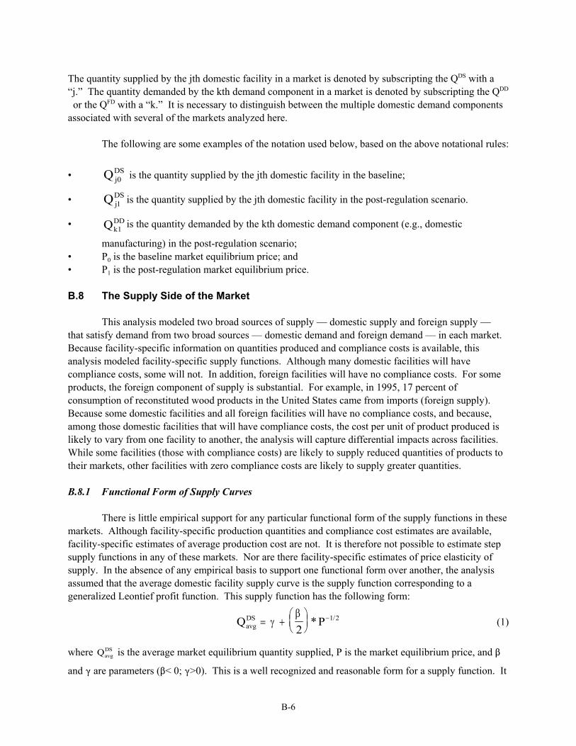
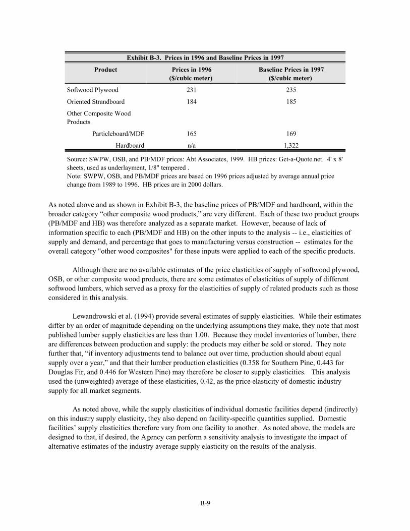
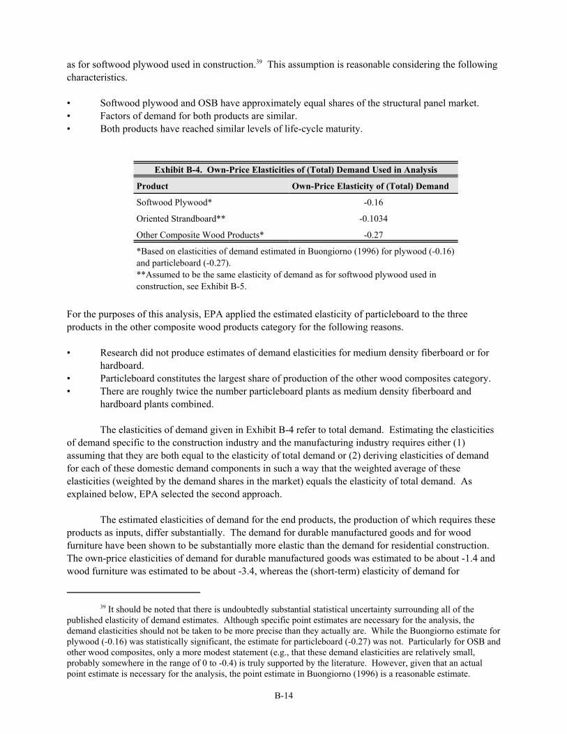
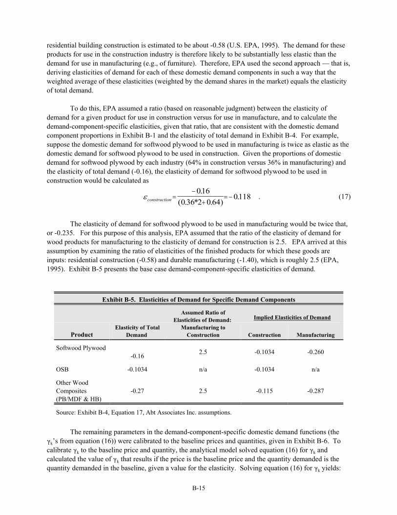
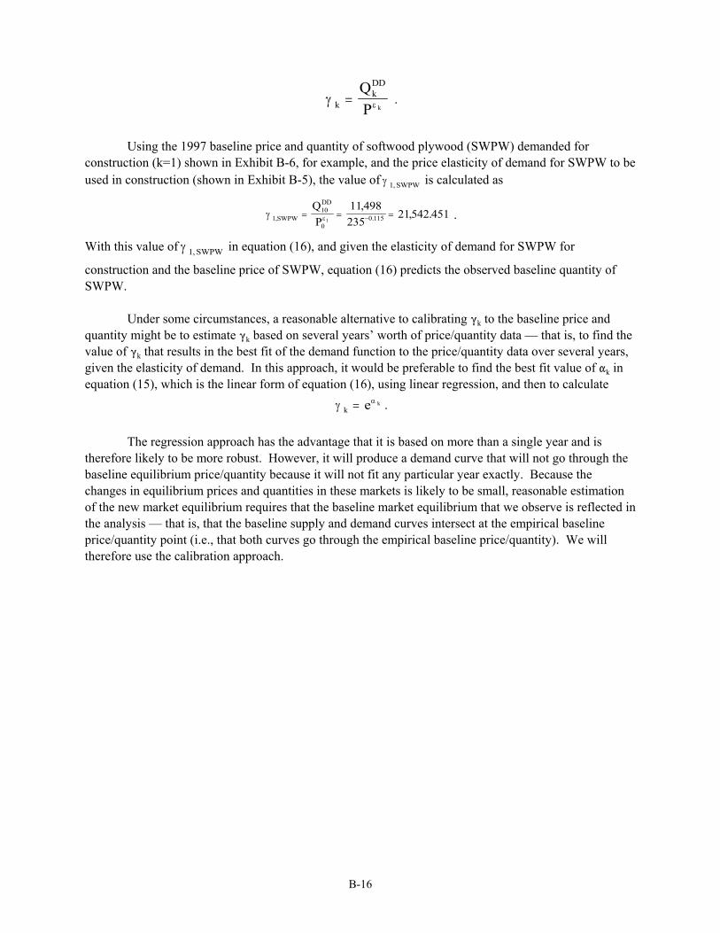

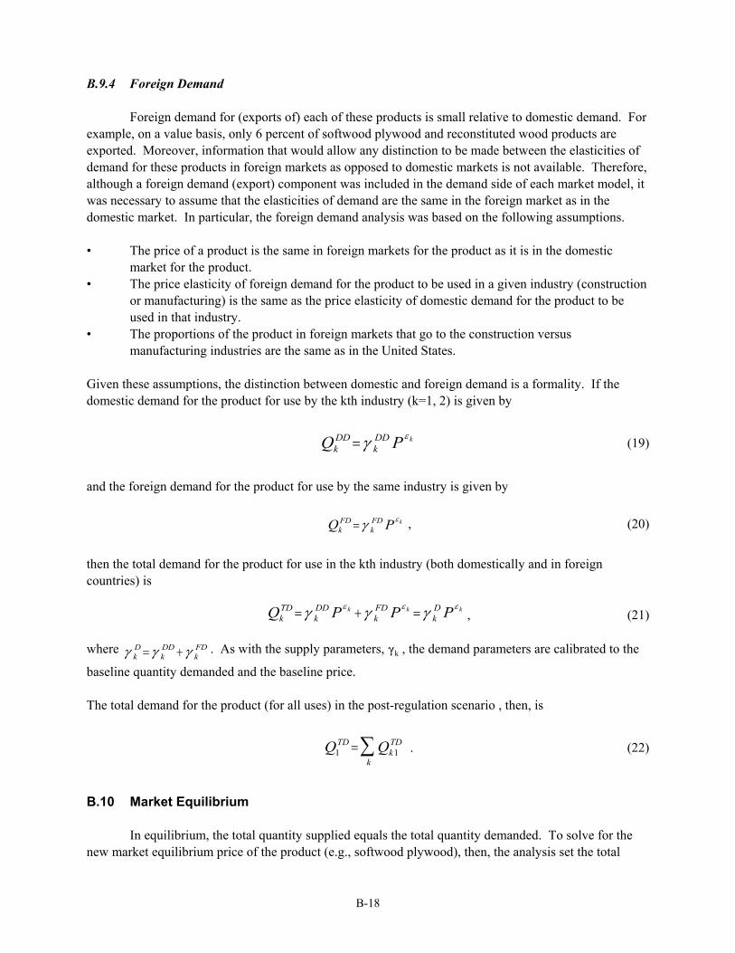
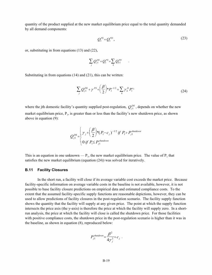


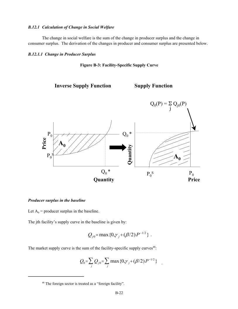
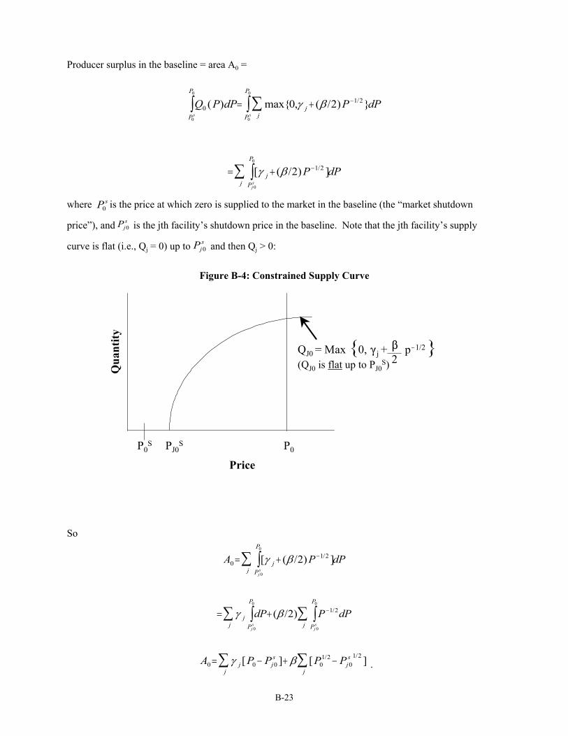
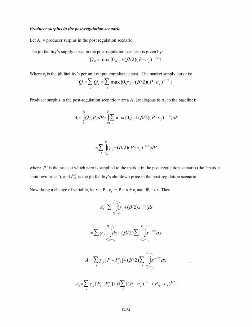

![Chronology,Narrative,andFoundingActs ...€¦[sic]-ajournalofliterature,cultureandliterarytranslation UtopiaandPoliticalTheology No.2-Year5 06/2015-LC.2 ISSN1847-7755;doi:10.15291/sic/2.5.lc.2](https://static.documents.pub/doc/80x56/5ac5edff7f8b9a12608de0ca/chronologynarrativeandfoundingacts-sic-ajournalofliteraturecultureandliterarytranslation.jpg)


![Chapter 2 SiC Materials and Processing Technology€¦ · 34 2 SiC Materials and Processing Technology Table 2.1 Key electrical parameters of SiC [1] Property 4H-SiC 6H-SiC 3C-SiC](https://static.documents.pub/doc/80x56/5f4fd11797ddad63bf719816/chapter-2-sic-materials-and-processing-technology-34-2-sic-materials-and-processing.jpg)
