1

 �ECONOMIC PLANTWIDE

CONTROL: �Control structure design for complete processing plants �

�Sigurd Skogestad

Department of Chemical EngineeringNorwegian University of Science and Tecnology (NTNU)Trondheim, Norway

13 Jan. 2017TexPoint fonts used in EMF. Read the TexPoint manual before you delete this box.: AAA

Salamanca, Spain, Feb. 2017

2

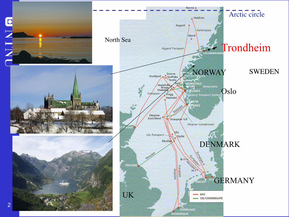
Trondheim

Oslo

UK

NORWAY

DENMARK

GERMANY

North Sea

SWEDEN

Arctic circle

3

Outline

•  Paradigm: based on time scale separation•  Plantwide control procedure: based on economics•  Example: Runner•  Selection of primary controlled variables (CV1=H y)

–  Optimal is gradient, CV1=Ju with setpoint=0–  General CV1=Hy. Nullspace and exact local method

•  Throughput manipulator (TPM) location•  Examples•  Conclusion

4

 �ECONOMIC PLANTWIDE CONTROL: Control structure design for complete processing plants �•  Sigurd Skogestad , Department of Chemical Engineering, Norwegian University

of Science and Technology (NTNU), Trondheim, Norway •  Abstract: A chemical plant may have thousands of measurements and control

loops. By the term plantwide control it is not meant the tuning and behavior of each of these loops, but rather the control philosophy of the overall plant with emphasis on the structural decisions. In practice, the control system is usually divided into several layers, separated by time scale: scheduling (weeks) , site-wide optimization (day), local optimization (hour), supervisory and economic control (minutes) and regulatory control (seconds). Such a hierchical (cascade) decomposition with layers operating on different time scale is used in the control of all real (complex) systems including biological systems and airplanes, so the issues in this section are not limited to process control. In the talk the most important issues are discussed, especially related to the choice of ”self-optimizing” variables that provide the link the control layers. Examples are given for optimal operation of a runner and distillation columns.

5

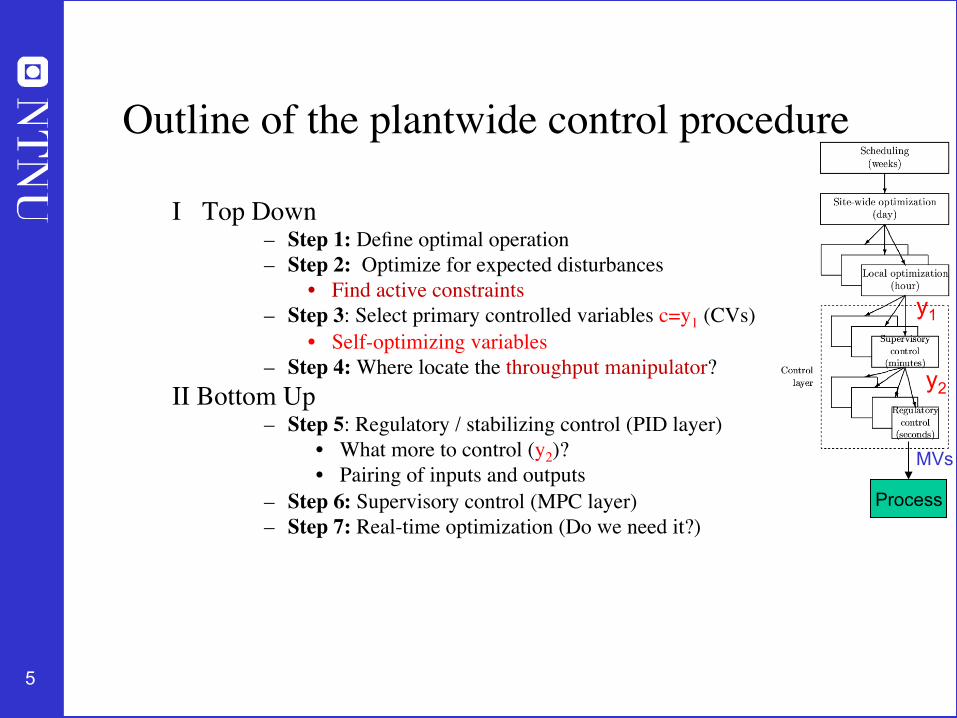
Outline of the plantwide control procedure

I Top Down –  Step 1: Define optimal operation–  Step 2: Optimize for expected disturbances

•  Find active constraints–  Step 3: Select primary controlled variables c=y1 (CVs)

•  Self-optimizing variables –  Step 4: Where locate the throughput manipulator?

II Bottom Up –  Step 5: Regulatory / stabilizing control (PID layer)

•  What more to control (y2)?•  Pairing of inputs and outputs

–  Step 6: Supervisory control (MPC layer)–  Step 7: Real-time optimization (Do we need it?)

y1

y2

Process

MVs

6

How we design a control system for a complete chemical plant?

•  Where do we start?•  What should we control? and why?•  etc.•  etc.

7

In theory: Optimal control and operation

Objectives

Present state

Model of system

Approach: • Model of overall system • Estimate present state • Optimize all degrees of freedom

Process control: •  Excellent candidate for centralized control

Problems:

•  Model not available •  Objectives = ? •  Optimization complex •  Not robust (difficult to handle uncertainty) •  Slow response time

(Physical) Degrees of freedom

CENTRALIZED OPTIMIZER

8

Practice: Engineering systems

•  Most (all?) large-scale engineering systems are controlled using hierarchies of quite simple controllers –  Large-scale chemical plant (refinery) –  Commercial aircraft

•  100’s of loops•  Simple components:

PI-control + selectors + cascade + nonlinear fixes + some feedforward

Same in biological systems

But: Not well understood

9

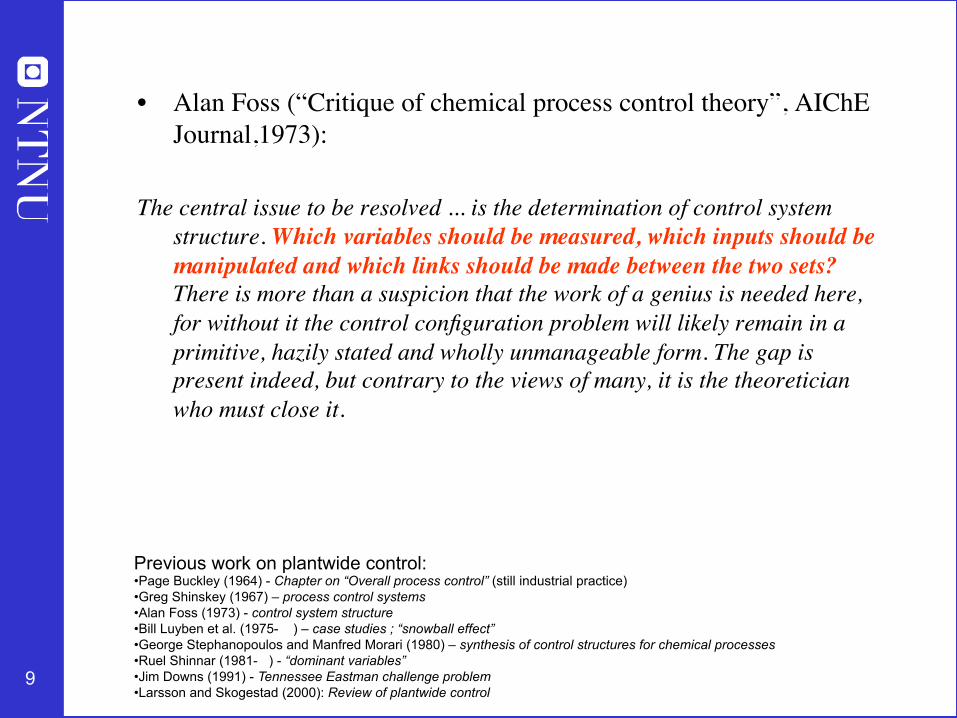
•  Alan Foss (“Critique of chemical process control theory”, AIChE Journal,1973):

The central issue to be resolved ... is the determination of control system structure. Which variables should be measured, which inputs should be manipulated and which links should be made between the two sets? There is more than a suspicion that the work of a genius is needed here, for without it the control configuration problem will likely remain in a primitive, hazily stated and wholly unmanageable form. The gap is present indeed, but contrary to the views of many, it is the theoretician who must close it.

Previous work on plantwide control: • Page Buckley (1964) - Chapter on “Overall process control” (still industrial practice) • Greg Shinskey (1967) – process control systems • Alan Foss (1973) - control system structure • Bill Luyben et al. (1975- ) – case studies ; “snowball effect” • George Stephanopoulos and Manfred Morari (1980) – synthesis of control structures for chemical processes • Ruel Shinnar (1981- ) - “dominant variables” • Jim Downs (1991) - Tennessee Eastman challenge problem • Larsson and Skogestad (2000): Review of plantwide control

10

Main objectives control system

1.  Economics: Implementation of acceptable (near-optimal) operation2.  Regulation: Stable operation

ARE THESE OBJECTIVES CONFLICTING?

•  Usually NOT –  Different time scales

•  Stabilization fast time scale–  Stabilization doesn’t “use up” any degrees of freedom

•  Reference value (setpoint) available for layer above•  But it “uses up” part of the time window (frequency range)

11

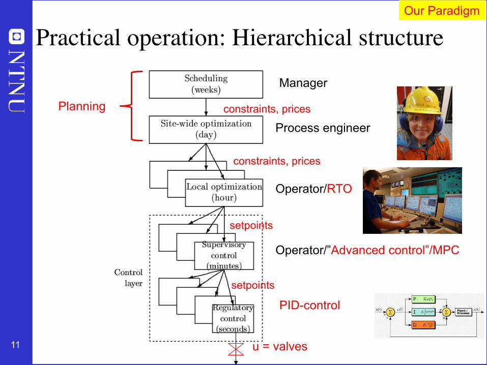
Practical operation: Hierarchical structure

Manager

Process engineer

Operator/RTO

Operator/”Advanced control”/MPC

PID-control

u = valves

Our Paradigm

setpoints

setpoints

constraints, prices

constraints, prices Planning

12

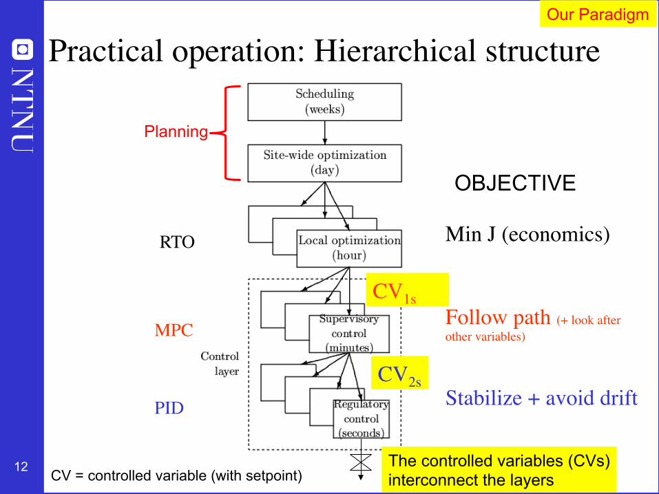
CV1s

MPC

PID

CV2s

RTO

Follow path (+ look after other variables)

Stabilize + avoid drift

Min J (economics)

u (valves)

OBJECTIVE

The controlled variables (CVs) interconnect the layers CV = controlled variable (with setpoint)

Our Paradigm

Practical operation: Hierarchical structure

Planning

13

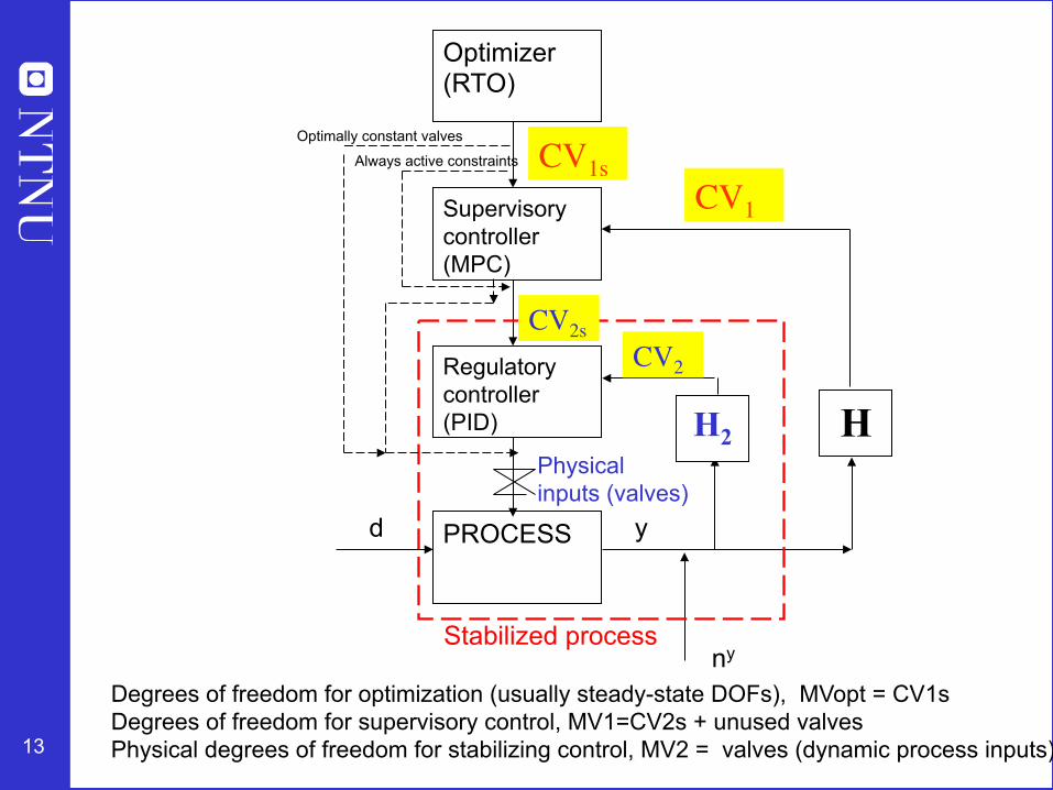
Degrees of freedom for optimization (usually steady-state DOFs), MVopt = CV1s Degrees of freedom for supervisory control, MV1=CV2s + unused valves Physical degrees of freedom for stabilizing control, MV2 = valves (dynamic process inputs)

Optimizer (RTO)

PROCESS

Supervisory controller (MPC)

Regulatory controller (PID) H2 H

y

ny

d

Stabilized process

Physical inputs (valves)

Optimally constant valves

Always active constraints CV1sCV1

CV2sCV2

14

Control structure design procedure

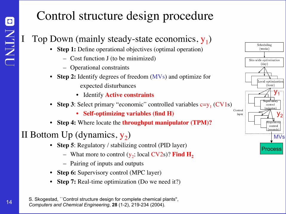
I Top Down (mainly steady-state economics, y1)•  Step 1: Define operational objectives (optimal operation)

–  Cost function J (to be minimized)–  Operational constraints

•  Step 2: Identify degrees of freedom (MVs) and optimize for expected disturbances

•  Identify Active constraints•  Step 3: Select primary “economic” controlled variables c=y1 (CV1s)

•  Self-optimizing variables (find H)•  Step 4: Where locate the throughput manipulator (TPM)?

II Bottom Up (dynamics, y2)•  Step 5: Regulatory / stabilizing control (PID layer)

–  What more to control (y2; local CV2s)? Find H2

–  Pairing of inputs and outputs•  Step 6: Supervisory control (MPC layer)•  Step 7: Real-time optimization (Do we need it?)

y1

y2

Process

MVs

S. Skogestad, ``Control structure design for complete chemical plants'', Computers and Chemical Engineering, 28 (1-2), 219-234 (2004).

15

Step 1. Define optimal operation (economics)

•  What are we going to use our degrees of freedom u (MVs) for?•  Define scalar cost function J(u,x,d)

–  u: degrees of freedom (usually steady-state)–  d: disturbances–  x: states (internal variables)Typical cost function:

•  Optimize operation with respect to u for given d (usually steady-state):

minu J(u,x,d)subject to:

Model equations: f(u,x,d) = 0Operational constraints: g(u,x,d) < 0

J = cost feed + cost energy – value products

16

Step S2. Optimize��(a) Identify degrees of freedom �(b) Optimize for expected disturbances

•  Need good model, usually steady-state•  Optimization is time consuming! But it is offline•  Main goal: Identify ACTIVE CONSTRAINTS•  A good engineer can often guess the active constraints

17

Step S3: Implementation of optimal operation

•  Have found the optimal way of operation. How should it be implemented?

•  What to control ? (CV1). 1.  Active constraints2.  Self-optimizing variables (for

unconstrained degrees of freedom)

18

–  Cost to be minimized, J=T–  One degree of freedom (u=power)–  What should we control?

Optimal operation - Runner

Optimal operation of runner

19

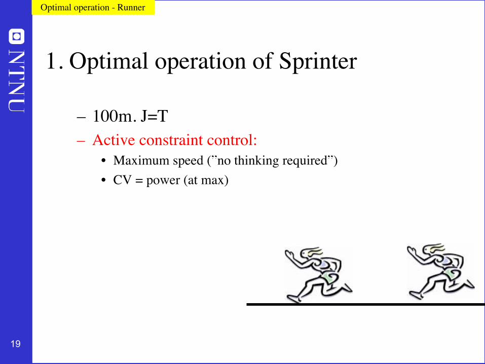
1. Optimal operation of Sprinter

–  100m. J=T–  Active constraint control:

•  Maximum speed (”no thinking required”)•  CV = power (at max)

Optimal operation - Runner

20

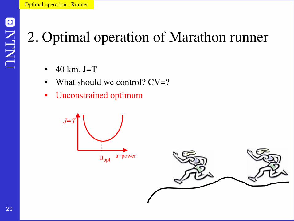
•  40 km. J=T•  What should we control? CV=?•  Unconstrained optimum

Optimal operation - Runner

2. Optimal operation of Marathon runner

u=power

J=T

uopt

21

•  Any self-optimizing variable (to control at constant setpoint)?

•  c1 = distance to leader of race•  c2 = speed•  c3 = heart rate•  c4 = level of lactate in muscles

Optimal operation - Runner

Self-optimizing control: Marathon (40 km)

22

�Conclusion Marathon runner

CV1 = heart rate

select one measurement

•  CV = heart rate is good “self-optimizing” variable •  Simple and robust implementation •  Disturbances are indirectly handled by keeping a constant heart rate •  May have infrequent adjustment of setpoint (cs)

Optimal operation - Runner

c=heart rate

J=T

copt

23

Summary Step 3. �What should we control (CV1)?

Selection of primary controlled variables c = CV1

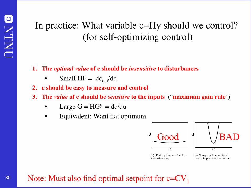
1.  Control active constraints!2.  Unconstrained variables: Control self-optimizing

variables!•  Old idea (Morari et al., 1980):

“We want to find a function c of the process variables which when held constant, leads automatically to the optimal adjustments of the manipulated variables, and with it, the optimal operating conditions.”

24

The ideal “self-optimizing” variable is the gradient, Ju

c = ∂ J/∂ u = Ju–  Keep gradient at zero for all disturbances (c = Ju=0)–  Problem: Usually no measurement of gradient

Unconstrained degrees of freedom

u

cost J

Ju=0 Ju<0

Ju<0

uopt

Ju 0

25

�

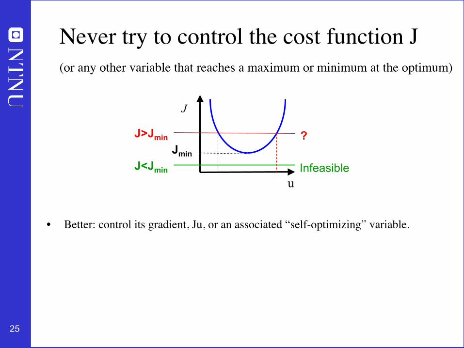
Never try to control the cost function J �(or any other variable that reaches a maximum or minimum at the optimum) �

•  Better: control its gradient, Ju, or an associated “self-optimizing” variable.

u

J

Jmin

J>Jmin

J<Jmin Infeasible

?

26

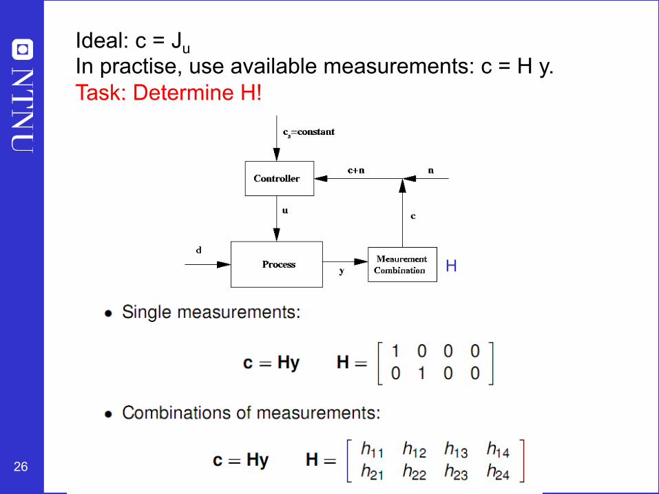
H

Ideal: c = Ju In practise, use available measurements: c = H y. Task: Determine H!

27

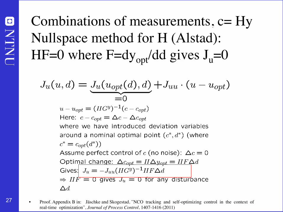
Combinations of measurements, c= Hy�Nullspace method for H (Alstad): �HF=0 where F=dyopt/dd gives Ju=0

•  Proof. Appendix B in: Jäschke and Skogestad, ”NCO tracking and self-optimizing control in the context of real-time optimization”, Journal of Process Control, 1407-1416 (2011)

•  .

28

“Minimize” in Maximum gain rule ( maximize S1 G Juu

-1/2 , G=HGy )

“Scaling” S1

“=0” in nullspace method (no noise)

With measurement noise

“Exact local method”

-  No measurement error: HF=0 (nullspace method) -  With measuremeng error: Minimize GFc

-  Maximum gain rule

29

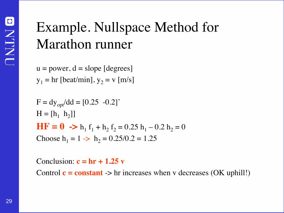
Example. Nullspace Method for Marathon runneru = power, d = slope [degrees]y1 = hr [beat/min], y2 = v [m/s]

F = dyopt/dd = [0.25 -0.2]’H = [h1 h2]]

HF = 0 -> h1 f1 + h2 f2 = 0.25 h1 – 0.2 h2 = 0Choose h1 = 1 -> h2 = 0.25/0.2 = 1.25

Conclusion: c = hr + 1.25 vControl c = constant -> hr increases when v decreases (OK uphill!)

30

BAD Good Good

Note: Must also find optimal setpoint for c=CV1

In practice: What variable c=Hy should we control?� (for self-optimizing control)

1.  The optimal value of c should be insensitive to disturbances •  Small HF = dcopt/dd

2.  c should be easy to measure and control 3.  The value of c should be sensitive to the inputs (“maximum gain rule”)

•  Large G = HGy = dc/du

•  Equivalent: Want flat optimum

31

Example: CO2 refrigeration cycle

J = Ws (work supplied)DOF = u (valve opening, z)Main disturbances:

d1 = TH d2 = TCs (setpoint) d3 = UAloss

What should we control?

pH

32

CO2 refrigeration cycle

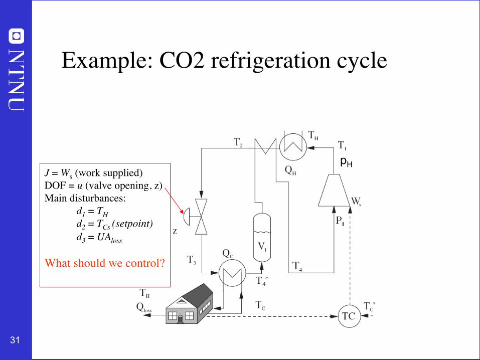
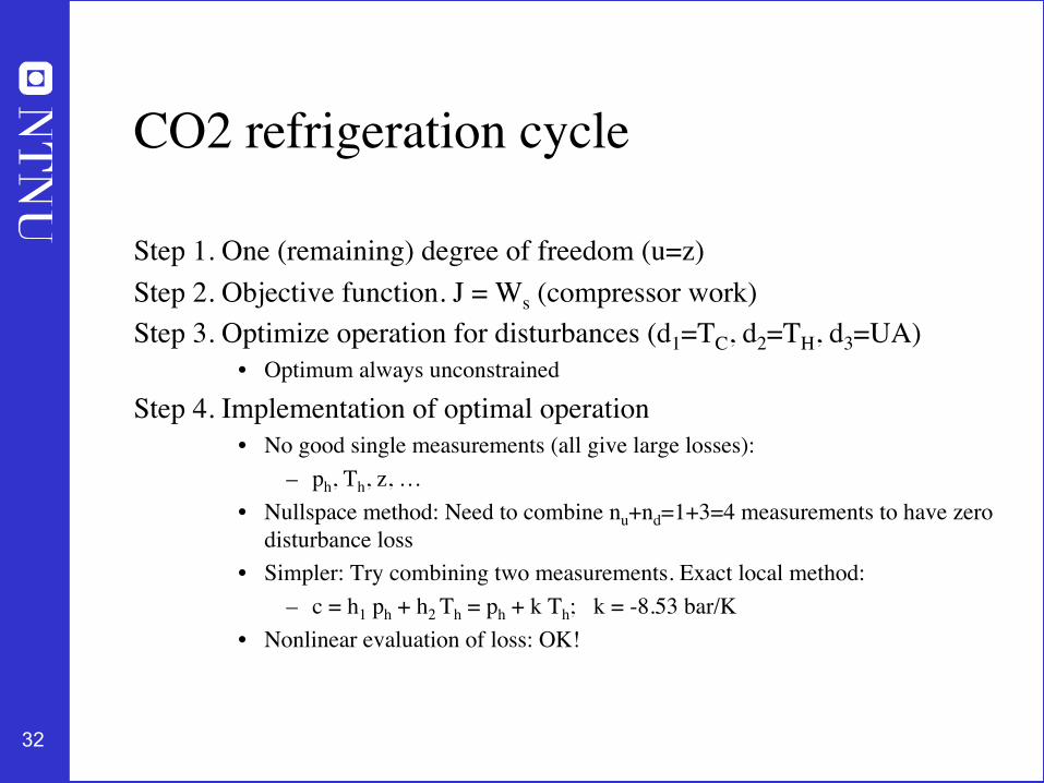
Step 1. One (remaining) degree of freedom (u=z)Step 2. Objective function. J = Ws (compressor work)Step 3. Optimize operation for disturbances (d1=TC, d2=TH, d3=UA)

•  Optimum always unconstrained

Step 4. Implementation of optimal operation•  No good single measurements (all give large losses):

–  ph, Th, z, …•  Nullspace method: Need to combine nu+nd=1+3=4 measurements to have zero

disturbance loss•  Simpler: Try combining two measurements. Exact local method:

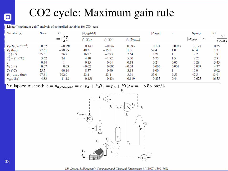
–  c = h1 ph + h2 Th = ph + k Th; k = -8.53 bar/K•  Nonlinear evaluation of loss: OK!

33

CO2 cycle: Maximum gain rule

34

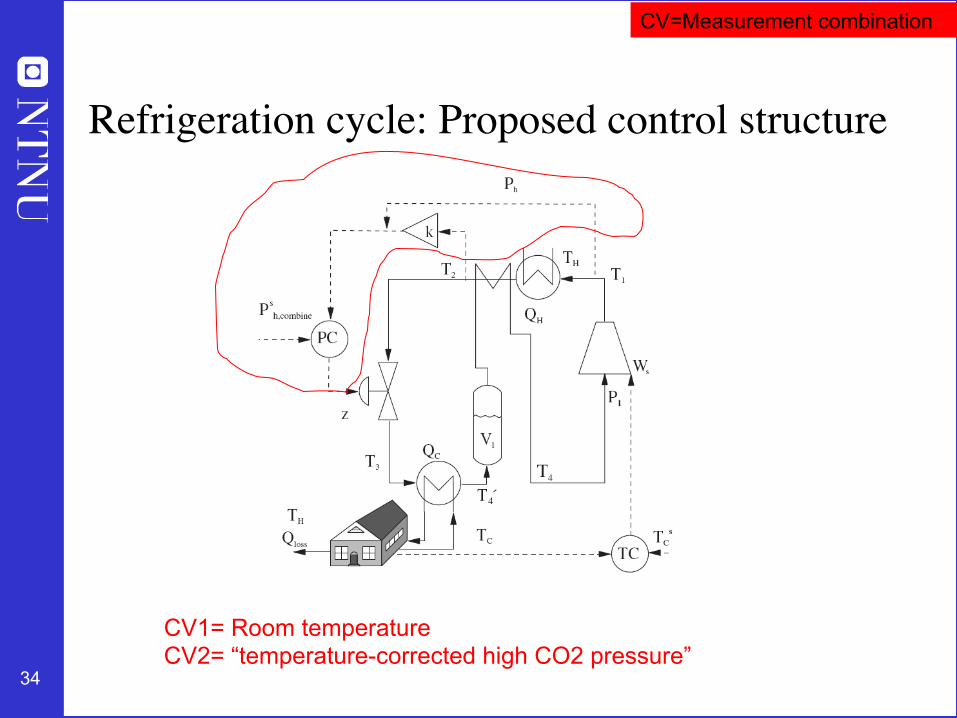
Refrigeration cycle: Proposed control structure

CV1= Room temperature CV2= “temperature-corrected high CO2 pressure”

CV=Measurement combination

35

Step 4. Where set production rate?

•  Where locale the TPM (throughput manipulator)?

– The ”gas pedal” of the process•  Very important!•  Determines structure of remaining inventory (level) control system•  Set production rate at (dynamic) bottleneck•  Link between Top-down and Bottom-up parts

•  NOTE: TPM location is a dynamic issue.Link to economics is to improve control of active constraints (reduce

backoff)

36

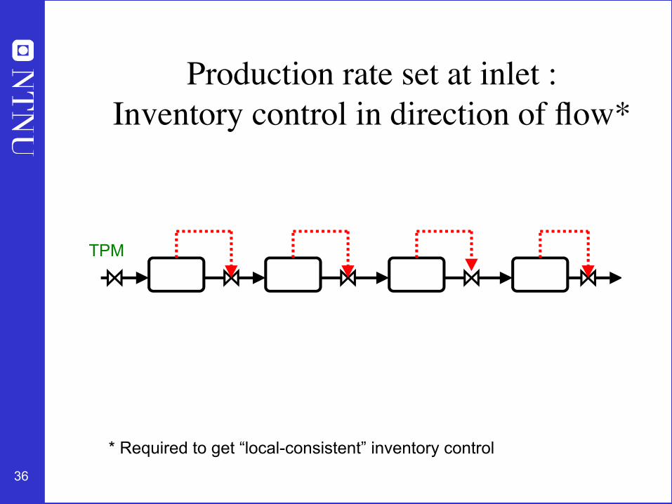
Production rate set at inlet :�Inventory control in direction of flow* �

* Required to get “local-consistent” inventory control

TPM

37

Production rate set at outlet:�Inventory control opposite flow

TPM

38

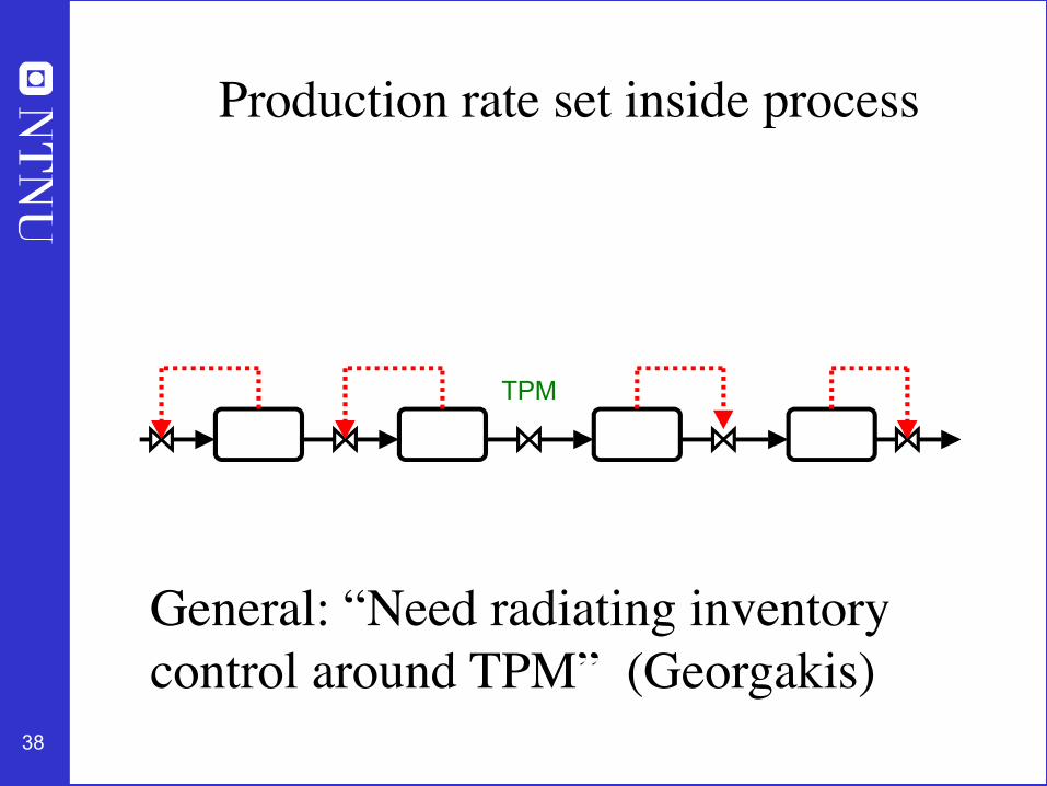
Production rate set inside process �

TPM

General: “Need radiating inventory control around TPM” (Georgakis)

39

CONSISTENT? QUIZ 1

40

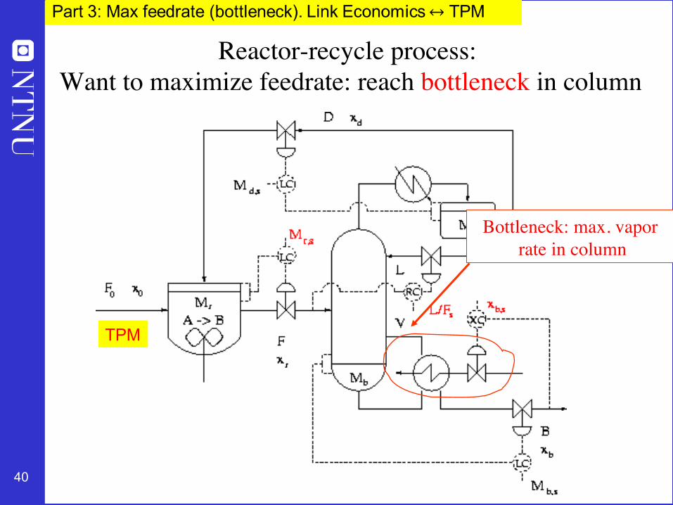
Reactor-recycle process:� Want to maximize feedrate: reach bottleneck in column

Bottleneck: max. vapor� rate in column

TPM

41

Reactor-recycle process with max. feedrate � Alt.A: Feedrate controls bottleneck flow

Bottleneck: max. vapor� rate in column

FC

Vmax

VVmax-Vs=Back-off = Loss

Vs

Get “long loop”: Need back-off in V

TPM

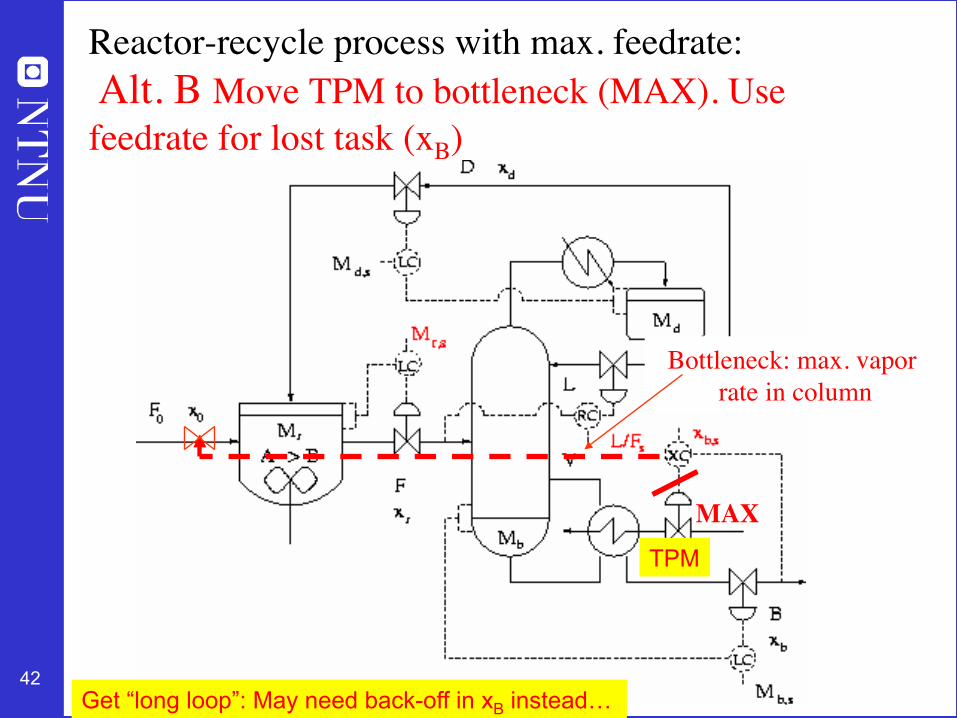
42

MAX

Reactor-recycle process with max. feedrate:� Alt. B Move TPM to bottleneck (MAX). Use feedrate for lost task (xB)

Get “long loop”: May need back-off in xB instead…

Bottleneck: max. vapor� rate in column

TPM

43

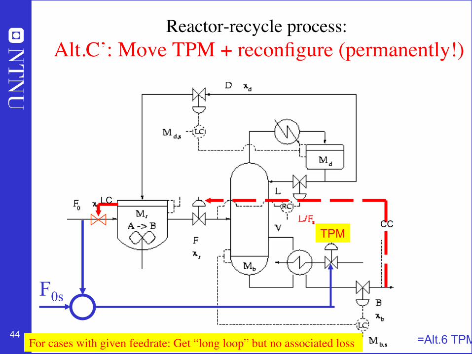
Reactor-recycle process with max. feedrate:� Alt. C: Best economically: Move TPM to bottleneck (MAX) + Reconfigure upstream loops

MAX

OK, but reconfiguration undesirable…

LC

TPM

44

Reactor-recycle process:� Alt.C’: Move TPM + reconfigure (permanently!)

F0s

For cases with given feedrate: Get “long loop” but no associated loss

LC

CC

=Alt.6 TPM

TPM

45

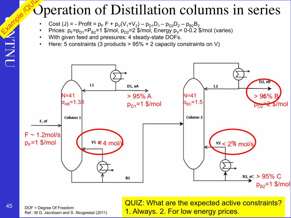
Operation of Distillation columns in series �

DOF = Degree Of Freedom Ref.: M.G. Jacobsen and S. Skogestad (2011)

> 95% B pD2=2 $/mol

F ~ 1.2mol/s pF=1 $/mol < 4 mol/s < 2.4 mol/s

> 95% C pB2=1 $/mol

N=41 αAB=1.33

N=41 αBC=1.5

> 95% A pD1=1 $/mol

QUIZ: What are the expected active constraints? 1. Always. 2. For low energy prices.

=

= =

•  Cost (J) = - Profit = pF F + pV(V1+V2) – pD1D1 – pD2D2 – pB2B2 •  Prices: pF=pD1=PB2=1 $/mol, pD2=2 $/mol, Energy pV= 0-0.2 $/mol (varies) •  With given feed and pressures: 4 steady-state DOFs. •  Here: 5 constraints (3 products > 95% + 2 capacity constraints on V)

46

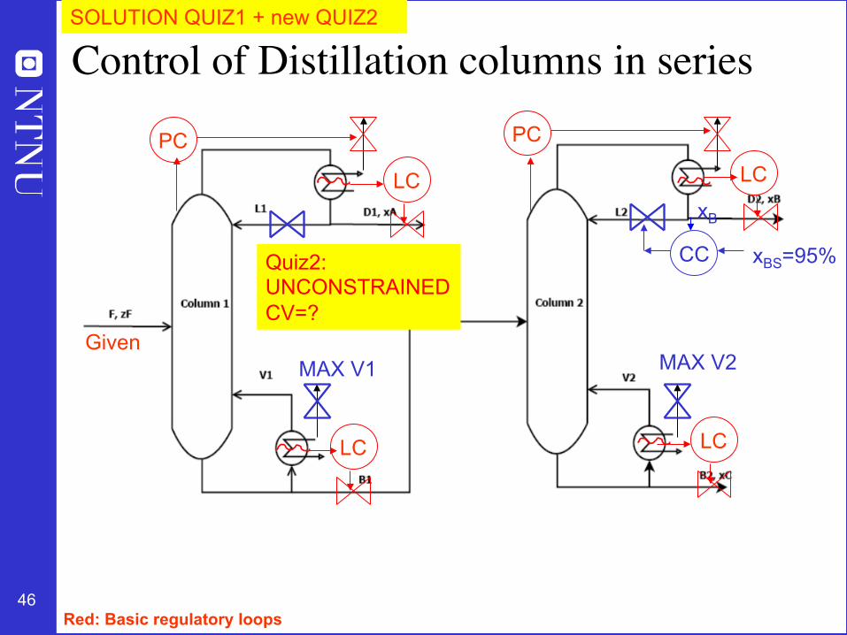
Control of Distillation columns in series �

Given

LC LC

LC LC

PC PC

Red: Basic regulatory loops

CC

xB

xBS=95%

MAX V1 MAX V2

SOLUTION QUIZ1 + new QUIZ2

Quiz2: UNCONSTRAINED CV=?

47

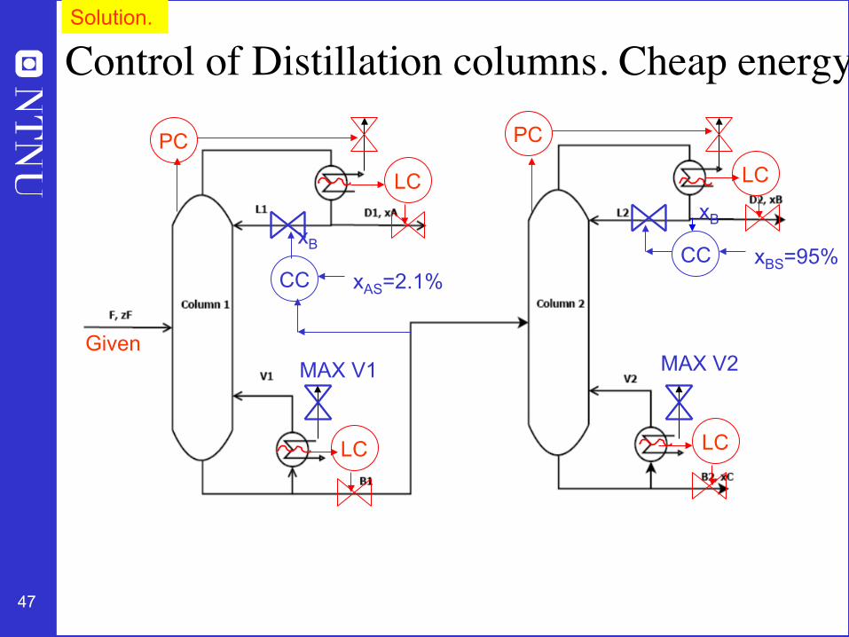
Given

LC LC

LC LC

PC PC

CC

xB

xBS=95%

MAX V1 MAX V2

CC

xB

xAS=2.1%

Control of Distillation columns. Cheap energy�Solution.

48

Active constraint regions for two �distillation columns in series

CV = Controlled Variable

3 2

0 1

1

0

2

[mol/s]

[$/mol]

1

Mode 1, Cheap energy: 3 active constraints -> 1 remaining unconstrained DOF (L1) -> Need to find 1 additional CVs (“self-optimizing”)

More expensive energy: Only 1 active constraint (xB) ->3 remaining unconstrained DOFs -> Need to find 3 additional CVs (“self-optimizing”)

Energy price

Distillation example: Not so simple

Mode 2: operate at BOTTLENECK. F=1,49 Higher F infeasible because all 5 constraints reached

Mode 1 (expensive energy)

49

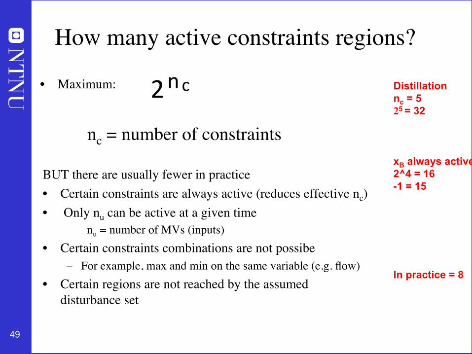
How many active constraints regions?

•  Maximum:

nc = number of constraints

BUT there are usually fewer in practice•  Certain constraints are always active (reduces effective nc)•  Only nu can be active at a given time

nu = number of MVs (inputs)•  Certain constraints combinations are not possibe

–  For example, max and min on the same variable (e.g. flow)•  Certain regions are not reached by the assumed

disturbance set

2nc Distillation nc = 5 25 = 32 xB always active 2^4 = 16 -1 = 15 In practice = 8

50

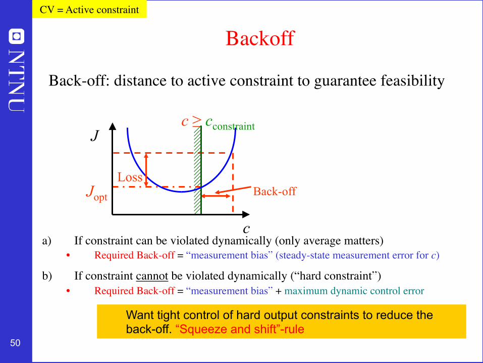
a)  If constraint can be violated dynamically (only average matters)•  Required Back-off = “measurement bias” (steady-state measurement error for c)

b)  If constraint cannot be violated dynamically (“hard constraint”) •  Required Back-off = “measurement bias” + maximum dynamic control error

Jopt Back-off Loss

c ≥ cconstraint

c

J

Backoff

Back-off: distance to active constraint to guarantee feasibility

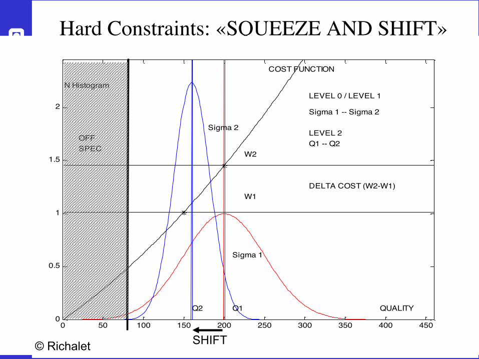
Want tight control of hard output constraints to reduce the back-off. “Squeeze and shift”-rule

The backoff is the “safety margin” from the active constraint and is defined as the difference between the constraint value and the chosen setpoint Backoff = |Constraint – Setpoint|

CV = Active constraint

51

Hard Constraints: «SQUEEZE AND SHIFT»

0 50 100 150 200 250 300 350 400 4500

0.5

1

1.5

2

OFF SPEC

QUALITY

N Histogram

Q1

Sigma 1

Q2

Sigma 2

DELTA COST (W2-W1)

LEVEL 0 / LEVEL 1

Sigma 1 -- Sigma 2

LEVEL 2Q1 -- Q2

W1

W2

COST FUNCTION

© Richalet SHIFT

SQUEEZE

CV = Active constraint

Rule for control of hard output constraints: • “Squeeze and shift”! • Reduce variance (“Squeeze”) and “shift” setpoint cs to reduce backoff

52

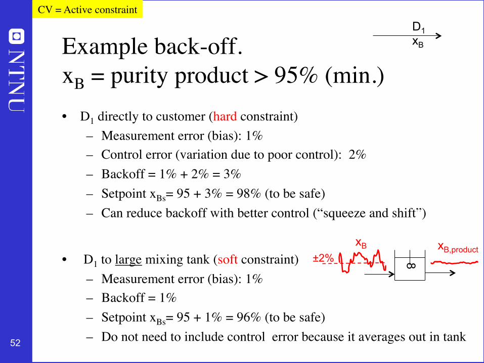
Example back-off. �xB = purity product > 95% (min.)•  D1 directly to customer (hard constraint)

–  Measurement error (bias): 1%–  Control error (variation due to poor control): 2%–  Backoff = 1% + 2% = 3%–  Setpoint xBs= 95 + 3% = 98% (to be safe)–  Can reduce backoff with better control (“squeeze and shift”)

•  D1 to large mixing tank (soft constraint)–  Measurement error (bias): 1%–  Backoff = 1%–  Setpoint xBs= 95 + 1% = 96% (to be safe)–  Do not need to include control error because it averages out in tank

CV = Active constraintD1 xB

8

xB xB,product ±2%

53

Optimal centralized Solution (EMPC)

Sigurd

Academic process control community fish pond

54

Conclusion:�Systematic procedure for plantwide control

•  Start “top-down” with economics: –  Step 1: Define operational objectives and identify degrees of freeedom–  Step 2: Optimize steady-state operation. –  Step 3A: Identify active constraints = primary CVs c. –  Step 3B: Remaining unconstrained DOFs: Self-optimizing CVs c. –  Step 4: Where to set the throughput (usually: feed)

•  Regulatory control I: Decide on how to move mass through the plant:•  Step 5A: Propose “local-consistent” inventory (level) control structure.

•  Regulatory control II: “Bottom-up” stabilization of the plant•  Step 5B: Control variables to stop “drift” (sensitive temperatures, pressures, ....)

–  Pair variables to avoid interaction and saturation•  Finally: make link between “top-down” and “bottom up”.

•  Step 6: “Advanced/supervisory control” system (MPC):•  CVs: Active constraints and self-optimizing economic variables +•  look after variables in layer below (e.g., avoid saturation)•  MVs: Setpoints to regulatory control layer.•  Coordinates within units and possibly between units

cs

http://www.nt.ntnu.no/users/skoge/plantwide

55

Summary and references•  The following paper summarizes the procedure:

–  S. Skogestad, ``Control structure design for complete chemical plants'', Computers and Chemical Engineering, 28 (1-2), 219-234 (2004).

•  There are many approaches to plantwide control as discussed in the following review paper: –  T. Larsson and S. Skogestad, ``Plantwide control: A review and a new

design procedure'' Modeling, Identification and Control, 21, 209-240 (2000).

•  The following paper updates the procedure: –  S. Skogestad, ``Economic plantwide control’’, Book chapter in V.

Kariwala and V.P. Rangaiah (Eds), Plant-Wide Control: Recent Developments and Applications”, Wiley (2012).

•  Another paper:–  S. Skogestad “Plantwide control: the search for the self-optimizing

control structure‘”, J. Proc. Control, 10, 487-507 (2000).•  More information:

http://www.nt.ntnu.no/users/skoge/plantwide