ECONOMIC REFORMS AND TECHNICAL EFFICIENCY …ECONOMIC REFORMS AND TECHNICAL EFFICIENCY PERFORMANCE...

ECONOMIC REFORMS AND TECHNICAL EFFICIENCY PERFORMANCE IN

INDIAN MANUFACTURING SECTOR

P. Sivakumar K. Uma Shankar Patnaik Research Fellow, Professor, Department of Economics, Department of Economics, University of Hyderabad, University of Hyderabad, Hyderabad 500 046. Hyderabad 500 046 India India E-mail: [email protected] E-mail: [email protected]

mailto:[email protected]

mailto:[email protected]

ECONOMIC REFORMS AND TECHNICAL EFFICIENCY PERFORMANCE IN

INDIAN MANUFACTURING SECTOR

P. Sivakumar and K. Uma Shankar Patnaik

ABSTRACT

This paper estimate and examine the technical efficiencies of Indian manufacturing sector

covering 144 three-digit industries for the period of 1973-74 to 1997-98. The main aim of

this study is to capture the behavior of technical efficiencies during the pre and post

reforms periods. By employing time-varying stochastic frontier production function in

the transcendental logarithmic form, this analysis identifies that there is a decreasing

trend in the technical efficiency level across industries and across time periods1. The

main finding of this study is that the industry specific inefficiency effects are the main

factor affecting the production process in achieving maximum feasible output than the

other random factors such as weather, luck, strikes etc. Also, this paper identifies that

during the post reforms period, technical efficiency is much lower than that of pre-reform

periods.

2

INTRODUCTION

Changes in the productivity levels are increasingly recognized as a major influence on a

host of macro and micro-economies problems. Politicians, industrialists, economists,

trade unionists and engineer all emphasis the importance of improving productivity

levels. The increasing attention paid to changes in the levels of productivity is probably

the results of persistent and high levels of inflation experienced in the past two decades as

well as increasingly competitive international market (Abby Ghobadian, 1990). The

literature abounds with rival definition of productivity. They range from ‘getting work

done’, ‘utilization of resources’, ‘reduction in cost’, ‘efficiency of resource allocation’ to

‘efficiency of production’. In broad terms, the definition of productivity falls into three

categories. These are the technological, engineering and economists concepts. The

technological concept defines productivity as the ratio of output to inputs expanded in its

production. The engineers view efficiency as the relationship between the actual and

potential output of the production process, while the economists define productivity as

the efficiency of the resource allocation.

An efficient and modern firm/industry is most likely to have lower cost of production,

improved quality of products and hence higher profits. Such a firm/industry can only be

competitive in the domestic as well as global market. It is well known that Technological

change or technical progress brings about production efficiencies, which in turn lead to

productivity growth. Production efficiencies may be brought about by technical,

allocative (price) or scale economies. Technical inefficiency refers to the failure of the

production unit to achieve the maximum possible output for a given level of input vector.

3

Allocative inefficiency, on the other hand, is associated with the sub-optimal choice of

the combination of inputs in the sense that the ratio of any two-factor prices is not equal

to the marginal rate of substitution between those two inputs. Scale

economies/diseconomies are associated with production carried on at scales either too

small or too large to minimize the cost of production. Thus, technological change,

technical efficiency and scale economies/diseconomies constitute the three major

technological characteristics of a firm / industry.

The industrial and the external sector of the Indian economy witnessed major changes in

their policy framework during 1990s when the government of India announced its new

industrial policy in June 1991. This industrial policy marked a major departure from the

earlier import substituting and regulation oriented industrial policy framework. One of

the major reforms in the industrial policy is the abolition of the complex system of

industrial licensing, under which new investors setting up new units or existing investors

undertaking major expansion had to obtain industrial license from the government.

Industrial licensing system was abolished in all the industries except in a small list of

strategic and potentially hazardous industries and in a few industries, which are referred

for the small-scale sector. The new policy also included many measures to improve the

performance of state owned enterprises. Entry of private sector firms into dereserved

industries create more competition and is expected to improve the performance of the

public sector firms. The incentive to improve performance is also being increased by a

conscious policy of phasing out budgetary support to fund losses in loss making

enterprises. Foreign Exchange Regulation Act, 1973 (FERA) was substantially

4

liberalised. All restriction on FERA companies in the matter of borrowing funds or

raising deposits in India as well as taking over or creating any interest in Indian

companies have been removed. There are number of studies to analysis these policy

changes and its impact on productivity, employment level and efficiency in Indian

manufacturing sector for various time periods.

Evidence on productivity in India as brought out by number of studies has been varied in

the estimation. For the period from 1960 to 1980, Golder’s (1986) estimation for Total

Factor Productivity Growth (TFPG) turned out to be 1.2 per cent per annum. Ahluwalia

(1991), however, in her study observed a decline in total factor productivity at the rate of

0.3 per cent per annum over the period of 1965-66 to 1979-80. Based on the National

Accounts Statistics another study done by Goldar(1995) estimated the total factor

productivity growth for the organized manufacturing sector at the rate of 1.55 per cent

per annum over the period 1970-71 to 1980-81 which rose to 3.85 per cent during 1980-

81 to1985-86 and further to 5.05 per cent during 1985-56 to 1990-91. The studies carried

out by the industrial Credit and Investment Corporation of India (ICICI, 1994) for

companies for which it provides assistance, estimated the growth rate of TFP at –2.7 per

cent per annum in the 1970s, -0.9 per cent per annum for the period from 1982-83 to

1986-87 and 2.1 per cent per annum during 1987-88 to 1991-92. Arup Mitra (1999), in

his study estimates technical efficiency for manufacturing industries across Indian states

using frontier production framework and observed deceasing trend in the technical

efficiency measures during the study period. Firm level study by Parameshwaran (2002)

for four major industry groups finds that there is decreasing trend in the efficiency levels

5

in all the four industries for the period of 1990 to 1997. He also finds that the reform

measures are not in favors of improving technical efficiency in Indian manufacturing

sector.

In view of these backgrounds, the present study aims at estimating technical efficiency

for Indian manufacturing sector at the three-digit level for the period of 1973-74 to 1997-

98. Since, for some of the industries the data relating to the WPI, capital and labour

inputs were not available for the whole sample period, we have considered 144 three-

digit industries for the analysis2. This study tries to explore the effects of reform

measures on technical efficiency scores during the pre and post liberalization scenario by

dividing the whole sample period into three sub periods (1973-74 to 1980-81, 1981-82 to

1990-91 and 1991-92 to 1997-98). Time varying stochastic frontier production function

and the estimation process are discussed in the following section. Section-III of this

paper briefly explains the data and variable used for this analysis. Section-IV and V

presents results and the main findings of the study.

THEORETICAL FRAMEWORK

Technical efficiency is a form of productive efficiency and is concerned with the

maximization of output for a given set of resource inputs. The measure of productive and

technical efficiency is based on the ‘best practice’ production function proposed by

Farrell (1957). Given the one output and two input framework, the efficient frontiers or

‘best practice’ production function can be expressed by the isoquant that shows the

6

minimum combination of inputs of a given quality given the state of technology that can

produce a specific level of output. Thus, in terms of production function, points on the

frontier are efficient and those below are inefficient (Chirwa, 2000).

Developments that followed Farrell’s approach to measure technical efficiency are

grouped into non-parametric frontiers and parametric frontiers. Non-parametric frontier

models in measuring technical efficiency do not impose any functional form on the

production frontiers and do not make any assumptions about the error term. These use

linear programming approaches and the most popular non-parametric approach is Data

Envelopment Analysis. Whereas, the parametric approaches impose a functional form on

the production function and assumptions are made about the data (Sankho Kim 2003).

The most common functional forms include the Cobb-Douglas, Constant Elasticity of

Substitution and Transcendental logarithmic production functions. The other distinction

in frontier measures is between deterministic and stochastic frontiers. Stochastic frontiers

assumes that the deviation from the frontier are due to partly to random events and partly

to industry / firm specific inefficiency and deterministic frontiers assumes that all the

deviations from the frontier are a results of industry / firm’s inefficiency.

The estimation of technical efficiency using econometric models can be categorized

according to the type of data employed; i.e., panel data or cross sectional data. Several

difficulties noted with the cross sectional stochastic frontier production frontier models in

the literature. The main problem is maximum likelihood estimation of stochastic

production frontier model, the subsequent separation of technical inefficiency from the

7

statistical noise, both requires strong distributional assumptions on each error component.

Also the robustness of inference to these assumptions is not well documented. Apart

from this maximum likelihood estimation also requires an assumption that the technical

inefficiency error component be independent of the regressors, although it is easy to

imagine that technical inefficiency might correlated with the input vectors producers

select (Schmidt and Sickles, 1984). These limitations can be avoided by employing panel

data. A panel data contains more information than a single cross-section. Having access

to panel data enables us to adopt conventional panel data estimation techniques to the

technical efficiency measurement problem. Moreover these techniques are not rest on

strong distributional assumptions. Also repeated observations on a sample of producers

can serve as a substitute for strong distributional assumptions. Moreover, adding more

observations on each producer generates information not provided by adding more

producers to a cross section (Kumbhakar 1990).

Two types of estimation techniques are found in the literature while using panel data, in

estimating technical efficiencies. The first technique in which, technical efficiency is

allowed to vary across producers, but it is assumed to be constant through time for each

producers, referred as time-invariant technical efficiency model. In the competitive

environment, it is hard to accept the notion that technical efficiency remain constant

through vary many time periods. The production frontier model, in which technical

efficiency is allowed to vary across producers and through time for each producer, is

referred as time-variant technical efficiency model.

8

Since our study employs 25 years of data for 144 three digit industries, the estimation of

technical efficiency in this paper follows time-varying model. The main advantage of this

is that, by estimating time-varying technical efficiency, one can test the other alternative

models and their suitability for the analysis.

The frontier production function can be expressed as

( )TExfy itit .: β= -----------------(1)

where, yit is the scalar output of producer i, i=1..2……..I , for the t period, t=1,2….T.

xit is the vector of N inputs used by the producer ‘i’,

( )β:itxf is the production frontier, and β is the vector of technology parameter

to be estimated.

The output oriented technical efficiency becomes,

( )β:it

it

xfy

TE = -------(2)

which defines technical efficiency as the ratio of observed output to the maximum

feasible output. The observed output (yit) achieves its maximum feasible value of

( )β:itxf , if, and only if TE=1. Otherwise TE<1 provides a measure of the shortfall of

observed output from maximum feasible output.

Now we begin by rewriting the equation (1) as,

( ) ( ititit uxfy −= exp: )β ----------(3)

Where TEi= . Since we require that ( itu−exp ) 1≤itTE , we have .0≥itu

The production function model will usually be linear in the logs of the variables, so the

equation (3) becomes,

9

----------(4) ∑ −+=n

itnitnit uxy lnln 0 ββ

where guarantees that .0≥itu ( )β:itit xfy ≤ .

Here uit=0 measures the technical efficiency,

uit>0 measures the technical inefficiency,

The objective is to obtain the estimates of the parameter vector β , which describes the

structure of the production function, and also to obtain estimates of the uit, which can be

used to obtain estimates of TE for each producers by means of TE= . Aigner,

Lovell and Schmidt (1977), and Meeusen and Van den Broeck(1977) simultaneously

introduced stochastic production frontier models. These models allow for technical

inefficiency, but they also acknowledge the fact that the random shocks outside the

control of producer can affect output. The great virtue of stochastic frontier models is that

the impact on outputs shocks due to variation in labour and machinery performance,

vagaries of the weather, and just plain luck can a least in principle be separated from the

combination of variation in technical efficiency.

( itu−exp )

)

If we again assume that ( β:itxf takes the log-linear form, then the stochastic

production frontier model can be written as

-------------(5) ∑ −++=n

ititnitnit uvxy lnln 0 ββ

where vit-is the two-sided ‘noise’ components, and uit is the non-negative technical

inefficiency component of the error term. As before, uit>0, but vit may take any value. A

symmetric distribution, such as the normal distribution is usually assumed for vit

10

From this equation the measures of the level of technical efficiency of the ith industry in

the tth period can be defined as the ratio of observed to the maximum possible output, i.e.

( )

( ) ( )it

itv

it

itu

exfy

eTEβ:

== − ---------- (6)

It is rational to argue that the reform policies can influence the industries with varying

degree of intensity, and consequently, the level of improvement in technical efficiency in

different industry would be different. Therefore, it becomes necessary to model uit

accordingly. If uit is remains constant over time, which indicates that there is no

improvement in technical efficiency. Alternatively, if uit decrease or increase, indicating

that technical efficiency may either improve or deteriorate over time

Following Battese and Coelli (1992), the above characteristics of technical efficiency can

be modeled as,

(( Ttuu iit −−= ))ηexp -------------(7)

Where the ui are independent random variables and η is an unknown parameter, which

represents the rate of changes in the technical inefficiency. It is expected that, uit

decrease, remain constant or increases as ‘t’ increases depending on whether η >0, η =0

or η <0, respectively. The case in which η is positive implies that, on average, industry

improve their level of technical efficiency over time. A negative value of η implies that

the industry’s efficiency worsens over time. Now the estimates of the industry-specific

technical efficiency require the assumption about the distribution of ui to facilitate the use

of maximum likelihood methods. It is assumed that ui is a non-negative truncation of

11

the ( )2, uN σμ . Further, uit and vit are assumed to be distributed independently (Kalirajan

1997).

However, neither uit nor vit can be obtained from the estimation and what is obtained is

the residualε , which is the sum of uit and vit. According to the statistical theory the best

predictor of an unknown random variable (uit), given the value of the combined random

variable (uit and vit), is the minimum mean-square error predictor obtained from the

conditional expectation of uit (Kalirajan and Shand 1999).

Following Battese and Coelli (1992)3, the logarithm of the likelihood function for the

sample observation is represented as

( ) ( ) ( ) ( ) ( )

( )[ ] ( )[ ]

( ) ( ) ( ) ( )∑∑∑

∑

∑∑∑

===

=

===

+−⎥⎦⎤

⎢⎣⎡ −′−−

−Φ−+−Φ−−

′+−−−⎥⎦

⎤⎢⎣

⎡−=

N

iii

N

i

N

iviiii

N

iii

N

iiiv

N

ivi

N

ii

NNxyxy

N

TTyL

1

2**

1

2

1

2

1

**

1

22

1

2

1

**

21

21

21

/1ln/1ln

ln21ln1

212ln

21;

σμσμσββ

σμσμ

σηησσπθ

----(8)

where ( )′′≡ ημσσβθ ,,,, 22*v

Using the re-parameterization, where and 222uv σσσ += 22 σσγ u= , the logarithm of

the likelihood function is expressed by

( ) ( ) ( ){ } ( ) ( )

( )[ ] ( )[ ] ([ ])

( ) ( ) ( )∑

∑∑

∑∑

=

==

==

⎥⎦⎤

⎢⎣⎡ −−′−−+

−Φ−+−−Φ−−−′+−

−−−+⎥⎦

⎤⎢⎣

⎡−=

N

iiiiii

N

ii

N

iii

N

ii

N

ii

xyxyNz

zNzzN

TTyL

1

22*

1

*2

1

1

2

1

*

121

21

1ln211ln11ln

21

1ln121ln2ln

21;

σγββ

γηη

γσπθ

------(9)

12

where ( ) ( ) 2122 ,,,,, γσμημγσβθ ≡′≡ z and

( ) ( )( ) ( )[ ]{ } 212

*

111

1

γηησγγ

βηγγμ

−′+−

−′−−=

ii

iiii

xyz

The minimum mean square error predictor of the technical efficiency of the ith firm at the

tth period is estimated as: ( itit uTE −= exp )

( )[ ] =iituE ε/exp[ ]

( ) ⎟⎠⎞⎜

⎝⎛ +−⎟

⎟⎠

⎞⎜⎜⎝

⎛

−Φ−

−Φ− 2*2***

***

exp1

1itit

ii

iiiit σημησμ

σμση ------(10)

where iε represent the (Ti ) vector of 1× itη ’s associated with the time periods observed

from the ith industry, and

22

22*

uiiv

uiivi σηησ

σεημσμ

′+

′−= , 22

222*

uiiv

uvi σηησ

σσσ

′+=

Where iη represents the (Ti ) vector of1× itη ’s associated with time periods observed for

the ith industry, and is the standard normal distribution function (Schmidt and C A Knox

Lovell (1980).

The mean technical efficiency of industry at the tth period given by

[ ]( ) ⎟

⎠⎞⎜

⎝⎛ +−

⎟⎟

⎠

⎞

⎜⎜

⎝

⎛

−Φ−

−Φ−= 22exp

11

uttu

uttTE σημη

σμσμση

------ (11)

If the industry effects are time invariant, then the mean technical efficiency is obtained

from the equation (11) by substituting 1=iη .

Thus the time-varying stochastic frontier approach explained above offers a better

methodology consistent with production theory to examine the pattern of technical

efficiency over period of time.

13

DATA AND METHODOLOGY

Two basic sources of production data are the Index of Industrial production (IIP) and

Annual Survey of Industries (ASI). The index deals with only selected products and

selected firms. ASI collects and provides industry wise data on value added, wages,

output, capital stock, depreciation etc, at current prices for the factory registered under

the Indian Factory Act 1945, i.e., those which use power and employ at least 10 workers

and those which do not use power and employ at least 20 workers.

To estimate technical efficiency level, annual data on value added, fixed capital, number

of workers etc., are collected for the organized manufacturing sector from the Annual

Survey of Industries for the period of 25 years from 1973-74 to 1997-98 for 144 three

digit industries. Data on value added and capital stock are on gross basis inclusive of

depreciation. Since the major changes in the classification of industries was introduced in

the year 1973-74, we choose this year as initial year for this analysis (Pushpa Triveti

2000).

Our estimation on gross value added function is based on single deflation method. The

WPI for the years 1973-74 to 1980-81 was given at the base 1970-71, whereas, rest of the

period the base year is 1980-81. The price index corresponding to the years 1973-74 to

1980-81 have therefore, converted into the 1980-81 base year before deflating the value

added series. Perpetual Inventory Method (PIM) is used to derive the measure of capital

input series. According to this method, capital stock for a given period is traced by

14

adding the previous investment starting from a benchmark year, converting to constant

value by a price index for capital asset. Following Benerji (1975), Goldar (1986) and

Balakrishnan and Pushpangadan (1994), double of the book value of the fixed capital is

taken as a measure of capital stock for the benchmark year.

Capital stock for the benchmark year is,

where t = 1973-74. ( tBK 20 = )

)

For the subsequent years, gross real investment has taken as a measure of capital stock.

The gross real investment for the year ‘t’ is obtained by,

----------(12) ( ttttt PDBBI /1 +−= −

where Bt is the book value of the fixed capital in the year ‘t’.

Bt-1 is the depreciation in the year ‘t’.

Pt is the index for machinery and machine tools for the tth year with base

year 1980-81.

The capital input, gross capital stock at the constant prices (1980-81) at the year ‘t’

derived as,

-------------------(13) ∑=

−+=t

iitt IKK

00

The labor input is used for the analysis is that the total employees including wage earners

and the salaried classes.

The more flexible functional form of production function, transcendental logarithmic

form has been used to estimate coefficients of production variables. The two inputs

stochastic frontier production function in the translog form is expressed as,

15

( ) ( )

( )( ) ( ) ( ) ititTTitLTitKTititKL

itLLitKKTitLitKit

uvTTLATKALAKA

LAKATLAKAVA

−++++

++++++=

2

220

21lnlnlnln

ln21ln

21lnlnln

ββββ

βββββα----(14)

where VA-Real value added at 1980-81 prices.

KA-capital stock at 1980-81 prices.

LA-number of workers.

T-time period., t=1,2,3……25 (1973-74 to 1997-98)

i=1,2,3,……144.

v is the stochastic error term affecting the production process..

u is the measure of technical inefficiency.

RESULTS AND DISCUSSION

The data used in this paper are an unbalanced panel consisting of annul-time series for

144 Indian manufacturing industries at 3-digit level during the period of 1973-74 to

1997-98, with a total of 3451 observations. The summery statistics for variables used in

the stochastic frontier production function in estimating technical efficiency are presented

in the table-1. The mean values presented in the table are the logarithmic value of value

added, capital and labour used in the actual estimation. The estimation has been carried

out in four periods including three sub-periods to capture the changes in the technical

efficiency. The second column of the table-1 shows the summery statistics for the whole

sample period (1973-74 to 1997-98). The other three columns presented in the table

shows the summery statistics for the variables used in the analysis for three sub periods

via.1973-74 to 1980-81, 1981-82 to 1990-91 and 1991-92 to 1997-98.

16

Table-1 Summery statistics for variables in the stochastic frontier production function for

Indian manufacturing industry Variables 1973-74 to

1997-98 1973-74 to 1980-81

1981-82 to 1990-91

1991-92 to 1997-98

Value added 8.3270 (1.8701)

7.7696 (1.7813)

8.3196 (1.8323)

9.0169 (1.8030)

Capital 8.0430 (1.9266)

7.6850 (1.9297)

8.0301 (1.8970)

8.4982 (1.8729)

Labour 9.4752 (1.5446)

9.2721 (1.5683)

9.4949 (1.5419)

9.6934 (1.4883)

Total observations

3451 1138 1379 934

Number of industries

144 144 144 144

Note: figures in parenthesis are standard deviations.

Hypothesis Test

The transcendental logarithmic production function, used in the estimation of technical

efficiency, allows us testing various hypotheses. The stochastic frontier production

function in the translog form, defined by equation (14), contains 10 β parameters and

four additional parameters associated with the distribution of vit and uit-random variables.

Maximum likelihood estimates for these parameters were obtained by using the computer

programme, developed by Tim Coelli (1996), FRONTIER 4.1. We estimated five basic

models using the frontier production function defined in equation (14).

1. Model-1 assumes that there is no technical inefficiency effect in the production

function, i.e., 0:0 === ημγH

2. Model-2 assumes that technical inefficiency is time-invariant, 0:0 =ηH .

3. Model-3 assumes that there is no technical change in the production function,

0:0 ==== TLTKTTTH ββββ

17

4. Model-4 assumes that technical progress is neutral, 0:0 == TLTKH ββ

5. Model-5 assumes that the production function is Cobb-Douglas form,

0:0 ==== TLTKLLKKH ββββ

The likelihood ratio test, a statistical test of goodness of fit between two models, used to

test null-hypothesis. It is defined that more complex models must differ from the simple

models only if the addition of one or more parameters. Adding additional parameters will

always results in higher likelihood scores. To determine, whether the difference in

likelihood scores among the two models is statistically significant, the degree of freedom

should be considered. In the LR test, the degree of freedom equals to the number of more

additional parameters in the more complex model. In general, the LR test statistics

approximately follows the chi-square distribution.

The likelihood ratio (LR) test statistics is given by

( ) ( )[ 102 HLHL −−= ]λ ---------------(15)

Where

L(H0)- value of log-likelihood function under the null hypothesis.

L(H1)- value of log-likelihood function under the alternative hypothesis.

if the null hypothesis is true, then the LR test statistics has approximately a chi-square

distribution with the degrees of freedom equals to the number of restrictions.

Table-2 presents the test results of various hypotheses for the total sample period and also

for the other three sub-periods. The estimated log-likelihood function value, calculated

LR test statistics and critical value to accept or reject the test statistics are presented in the

18

table for the different sample periods. In the case of whole sample period all the null-

hypothesis are rejected at 1 % significant level. The null hypothesis that the there is no

technical inefficiency is rejected at 1% level for period-I, period-II and Period-III.

Table-2 Test of hypothesis for parameters of the distribution of technical efficiency

Null Hypothesis Log-likelihood Function

LR-Test Statistics

Critical Value

Decision

Whole sample period (1973-74 to 1997-98) 0:0 === ημγH -2905.844 2712.2452 10.50 Reject

0:0 =ηH -1634.060 169.3421 6.63 Reject 0:0 ==== TKTLTTTH βββα -1673.085 247.3839 13.28 Reject

0:0 == TKTLH ββ -1598.031 48.6423 9.21 Reject 0:0 ==== TTLKKKLLH ββββ -1667.956 118.5672 13.28 Reject

Period-I (1973-74 to1980-81) 0:0 === ημγH -780.6721 1013.0041 10.50 Reject

0:0 =ηH -274.4909 0.6414 6.63 Accept 0:0 ==== TKTLTTTH βββα -294.9299 41.5194 13.28 Reject

0:0 == TKTLH ββ -274.5816 0.8228 9.21 Accept 0:0 ==== TTLKKKLLH ββββ -331.8111 115.2818 13.28 Reject

Period-II (1981-82 to1990-91) 0:0 === ημγH -1073.951 980.5456 10.50 Reject



Period-III (1991-92 to1997-98) 0:0 === ημγH -965.9869 967.0924 10.50 Reject



Note: These models are estimated using Frontier 4.1 computer program.

19

Based on the critical value it is accepted that there is a technical inefficiency levels,

which are affecting the production process in order to achieve the maximum feasible

output in Indian manufacturing sector during the whole sample period and also during

other three sub-periods. The second null-hypothesis is that, the technical inefficiency is

time-invariant is rejected during the period of 1973-74 to 1997-98, thereby accepting that

technical inefficiency is varying across time periods. In the case of other three sub-

periods, this null hypothesis is accepted, indicating that technical inefficiency is constant

across periods, given the time-varying specification of the stochastic frontier production

function. The third null hypothesis that there is no technical progress in Indian

manufacturing industry is rejected at 1 % significant level and accepting that the

existence of technical change in the production process during all the sample periods

considered for the analysis.

The fourth hypothesis, technical progress is neutral is rejected at the whole sample period

study, whereas it is accepted at the other three sub-periods. It is evident from the results

that during three study period, the technical progress is found to be non-neutral in Indian

manufacturing sector. The last hypothesis is that, the technology in Indian manufacturing

sector is a Cobb-Douglas for, is rejected for the whole sample period and also for the

other three sub-periods. Thus, the Cobb-Douglas production function is not an adequate

specification for the Indian manufacturing sector, given the assumptions of the translog

production function.

20

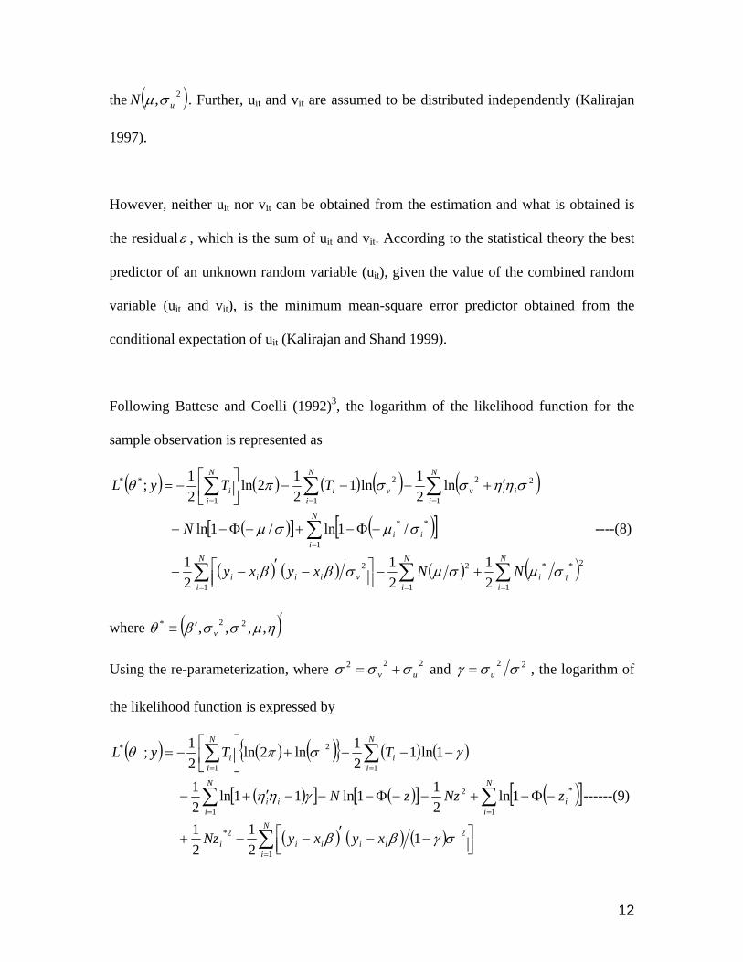
Estimates of frontier production function

The maximum likelihood estimates of frontier production function in the transcendental

logarithmic specification for the period of 1973-73 to 1997-98 are presented in the table-

3. In the table we have reported only two models out of five models estimated and also

the full model represents the estimation of all the parameters. The estimated model-I is

similar to that of OLS, since there is no technical inefficiency effects are considered for

the analysis. The model-I shows that the estimates of average production function, in

which the parametersμ , η and γ are restricted to be zero, indicating that there is no

technical inefficiency effects in the production function. Model-II represents the

technical inefficiency is time-invariant, indicating that there is no change in the technical

inefficiency levels across time periods in the industries. Full Model represents the full

frontier production function, expressing the existence of technical inefficiency,

technological progress and the time-varying effects of technical inefficiency in the given

stochastic frontier production function of transcendental logarithmic specification. Based

on the log-likelihood ratio test, the column 5 of the table-3 (full model) indicates the

existence of the time-varying technical inefficiency in Indian manufacturing industry

over the period of 1973-74 to 1997-98. From the table it is evident that all the coefficients

are significant at 1 % level. The significance of variance parameter and the ratio

variance parameter

2σ

γ implies that the realized output differ from potential output

significantly and the difference are mainly due to the differences in the industry-specific

technical inefficiency effects and not to any random change factors.

21

Table-3 ESTIMATES OF STOCHASTIC FRONTIER PRODUCTION FUNCTION USING

MAXIMUM LIKELIHOOD METHOD (1973-74 to 1997-98)

Sl.No Variables Parameters Model-I(OLS)

Model-II(MLE)

Full Model (MLE)

1 Constant 0α -5.2081 (19.20)

-1.0137 (3.06)

-1.8178 (5.83)

2 Capital Kβ 0.2004 (3.94)

0.2478 (4.99)

0.3668 (7.54)

3 Labour Lβ 1.7483 (21.72)

1.0759 (12.92)

1.0487 (12.17)

4 Capital*capital KKβ 0.1037 (13.03)

0.0436 (4.93)

0.0491 (6.03)

5 Labour*labour LLβ -0.1109 (9.62)

-0.0041 (0.29)

-0.0120 (0.82)

6 Kapital*labour KLβ -0.0436 (5.75)

-0.0405 (4.12)

-0.0425 (4.56)

7 Time Tβ -0.0259 (2.65)

-0.0035 0.53)

0.0224 (3.16)

8 Time*capital TKβ -0.0082 (7.13)

-0.0013 (1.66)

-0.0098 (10.26)

9 Time*labour TLβ 0.0111 (7.83)

0.0032 (3.29)

0.0095 (8.69)

10 Time*time TTβ 0.0016 (3.88)

0.0021 (7.14)

0.0035 (11.09)

11 222uv σσσ += 0.3165 0.5511

(17.55) 0.8333 (23.21)

12 ( )222uvu σσσγ += 0 0.7758

(69.14) 0.8529 (85.10)

13 μ 0 1.3077 (16.37)

1.6862 (14.38)

14 η 0 0 -0.0272 (14.53)

15 Log-Likelihood Function

-2905.84 -1675.79 -1590.18

Note: figures in parenthesis are ‘t’ statistics. The parameters are estimated using computer programme FRONTIER 4.1

However, the asymptotic t-test on the estimated value found to be 14.38, which is

significant at 1 % level, indicating that the mean of technical inefficiency is significantly

differ from zero. The result implies that the inclusion of ‘u’ in the production function

μ

22

equation is valid, and the assumption that ‘u’ follows a truncated normal distribution

with ( )2, uN σμ , and ‘u’ does not follows the normal distribution ( )2,0 uN σ . The time

varying technical (in)efficiency parameter η is found to be negative to the tune of

0.0272, which is significant at 1 % level indicating that the technical efficiency is

decreasing over the sample period in Indian manufacturing industry. It implies that the

rate of growth of technical efficiency in Indian manufacturing sector during 1973-74 to

1997-98 found to be decreasing to the extent of 2.72 per cent.

Given the specification of full model in which technical efficiency is found to be time-

varying with truncated distribution, the technical efficiencies of the individual industries

are calculated using minimum mean square predictor explained in equation (12). We

have estimated technical efficiencies for all the 144 three-digit industries for each time

period covering from 1973-74 to 1997-98 and reported only the average technical

efficiency levels in the table-4.

Since, the technical efficiency coefficient is found to be negative; the decreasing trends in

the estimated technical efficiencies scores are observed in the table. It is clear from the

analysis that overall average level of technical efficiency is found to be 31.61 % in Indian

manufacturing sector, implies that around 68 % of industry specific inefficiency effects

are affecting the production process in achieving the maximum feasible output. Also, the

causes for inefficiency levels in the manufacturing industry in India is mainly due to the

industry specific effects, but not the other stochastic effects such as, luck, whether, strikes

and lock-outs.

23

Table-4 Predicted average technical efficiencies of manufacturing industry in India

year TE Year TE year TE 1973-74 0.4218 1982-83 0.3401 1991-92 0.2626 1974-75 0.4118 1983-84 0.3257 1992-93 0.2502 1975-76 0.4016 1984-85 0.3216 1993-94 0.2448 1976-77 0.3941 1985-86 0.3194 1994-95 0.2438 1977-78 0.3852 1986-87 0.3059 1995-96 0.2323 1978-79 0.3775 1987-88 0.2999 1996-97 0.2268 1979-80 0.3679 1988-89 0.2899 1997-98 0.2233 1980-81 0.3548 1989-90 0.2819 1981-82 0.3485 1990-91 0.2703

Average TE

0.3161

Note: the estimates are computed using the computer programme FRONTIER 4.1, and these results are only the average TE of 144 three-digit industries for each period mentioned above.

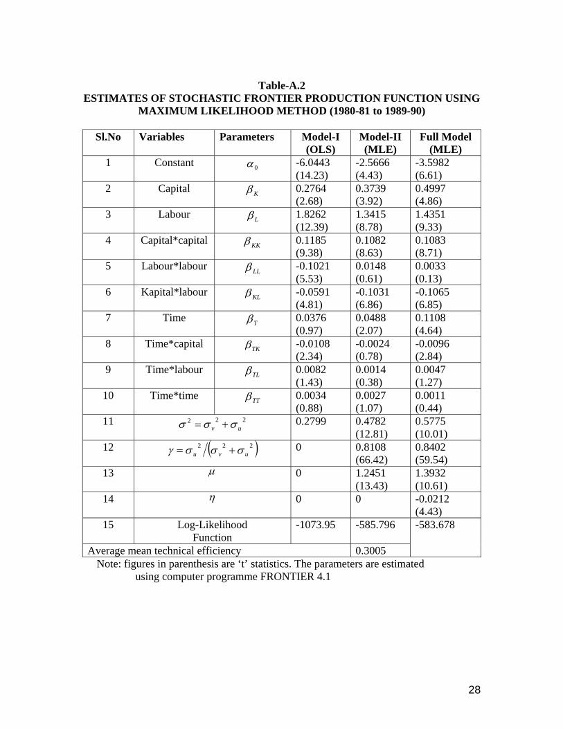
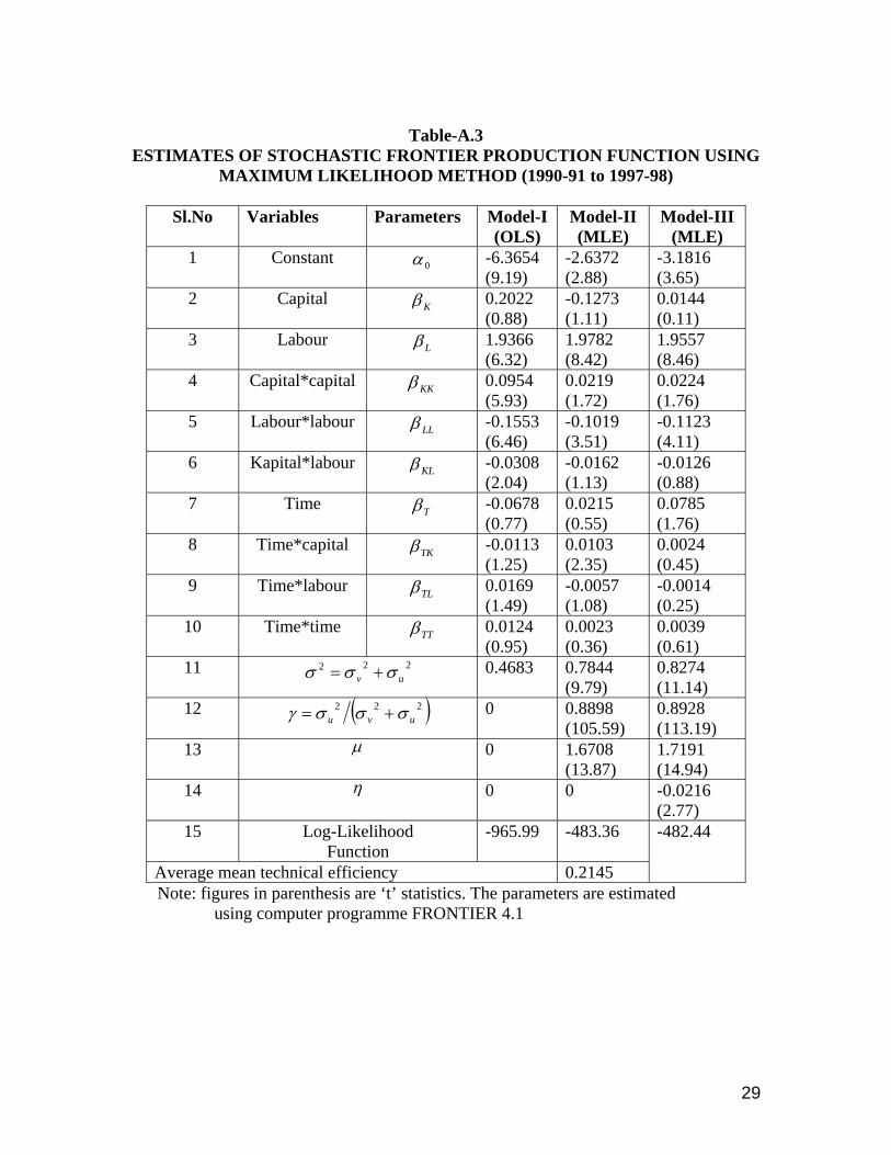
In order to capture the effects of reform policies on technical efficiency levels, we

estimated the parameters of the stochastic frontier production function in the

transcendental logarithmic form for three sub-periods, covering from 1973-74 to 1980-

81, 1981-82 to 1990-91 and 1991-92 to 1997-98. The results were presented in the

appendix-I, II, and III. From the results it is found that the technical efficiency is time-

invariant in all the three sub-periods, implying that there are no changes in the technical

efficiency scores during the three study periods. As we discussed earlier, in the time-

invariant model, the technical efficiency vary only across industries but it is not allowed

to vary over time periods. Hence, using the equation (11) we estimated mean technical

efficiency for each industry for the three different periods and reported the average of this

mean technical efficiency. It is evident from the results that technical efficiency is found

to be 28.84 % during 1973-74 to 1980-81, implies that around 71 % of inefficiency

effects are affecting the production process in Indian manufacturing industries. During

1981-82 to 1990-91, the level of technical efficiency is estimated as 30.05 %, implies that

there is increase in the TE compare with the earlier periods. In the post liberalization

24

period, 1991-92 to 1997-98, the estimated technical efficiency is 21.45 %, which is less

compare with the other two sub-periods. From the estimated results for the three

different sub-periods, the technical efficiency during the post reforms periods is much

less than the other two periods, implies that the reforms policies are not influencing in

increasing technical efficiency in Indian manufacturing industries.

CONCLUDING REMARKS

This paper estimates the technical (in)efficiency levels of the Indian manufacturing

sector using a sample of 144 three-digit industries for the period of 1973-74 to 1997-98

by employing time-varying stochastic frontier production function of transcendental

logarithmic form. The estimates of technical efficiencies are found to be time-varying

across industries and across time periods, for the whole sample period study. The study

reveals that there is a decreasing trend in the technical efficiency levels in Indian

manufacturing sector during the entire sample period. The empirical results of this study

suggest that the realized output differ from the potential output significantly in Indian

manufacturing sector and the differences are mainly due to the difference in the industry-

specific technical inefficiency effects than the other stochastic random factors. The

estimates for the three time periods (1973-74 to 1980-81, 1981-82 to 1990-91 and 1991-

92 to 1997-98), reveals that technical efficiency scores are constant across sample

periods, implies that there is no significant changes in the levels of technical efficiencies.

The estimated average mean technical efficiency is found to be lower during the period

1991-92 to 1997-98 as compare with the other two periods. Also, the study finds that

25

there exist of neutral technical progress during all three time periods in Indian

manufacturing sector. In concluding, the post reform period has negative impact on

Indian manufacturing sector with respect of its technical efficiency performance.

26

APPENDIX

Table-A.1 ESTIMATES OF STOCHASTIC FRONTIER PRODUCTION FUNCTION USING

MAXIMUM LIKELIHOOD METHOD (1973-74 to 1979-80)

Sl.No Variables Parameters Model-I(OLS)

Model-II(MLE)

Full Model (MLE)

1 Constant 0α -3.8867 (10.09)

-1.4454 (3.08)

-1.7975 (4.01)

2 Capital Kβ 0.2586 (3.38)

0.2385 (2.71)

0.2637 (2.81)

3 Labour Lβ 1.4453 (12.13)

1.1764 (9.94)

1.2289 (9.89)


0.0815 (5.77)

0.0987 (7.08)


-0.0082 (0.33)

0.0039 (0.15)


-0.0608 (3.34)

-0.0812 (4.34)

7 Time Tβ -0.0853 (1.79)

-0.0134 (0.49)

0.0123 (0.44)


-0.0022 (0.61)

-0.0006 (0.17)


0.0087 (1.98)

0.0059 (1.36)

10 Time*time TTβ -0.0019 (0.31)

-0.0069 (1.89)

-0.0079 (2.17)

11 222uv σσσ += 0.2329 0.4438

(11.53) 0.4311 (10.89)

12 ( )222uvu σσσγ += 0 0.8713

(104.85) 0.8691 (101.56)

13 μ 0 1.2437 (13.07)

1.2242 (12.69)

14 η 0 0 -0.0063 (0.95)


-780.67 -274.49

Average mean technical efficiency 0.2884

-274.17


27

Table-A.2

ESTIMATES OF STOCHASTIC FRONTIER PRODUCTION FUNCTION USING MAXIMUM LIKELIHOOD METHOD (1980-81 to 1989-90)

Sl.No Variables Parameters Model-I

(OLS) Model-II (MLE)

Full Model (MLE)

1 Constant 0α -6.0443 (14.23)

-2.5666 (4.43)

-3.5982 (6.61)

2 Capital Kβ 0.2764 (2.68)

0.3739 (3.92)

0.4997 (4.86)

3 Labour Lβ 1.8262 (12.39)

1.3415 (8.78)

1.4351 (9.33)


0.1082 (8.63)

0.1083 (8.71)


0.0148 (0.61)

0.0033 (0.13)


-0.1031 (6.86)

-0.1065 (6.85)

7 Time Tβ 0.0376 (0.97)

0.0488 (2.07)

0.1108 (4.64)


-0.0024 (0.78)

-0.0096 (2.84)


0.0014 (0.38)

0.0047 (1.27)

10 Time*time TTβ 0.0034 (0.88)

0.0027 (1.07)

0.0011 (0.44)

11 222uv σσσ += 0.2799 0.4782

(12.81) 0.5775 (10.01)

12 ( )222uvu σσσγ += 0 0.8108

(66.42) 0.8402 (59.54)

13 μ 0 1.2451 (13.43)

1.3932 (10.61)

14 η 0 0 -0.0212 (4.43)


-1073.95 -585.796


-583.678


28

Table-A.3

ESTIMATES OF STOCHASTIC FRONTIER PRODUCTION FUNCTION USING MAXIMUM LIKELIHOOD METHOD (1990-91 to 1997-98)

Sl.No Variables Parameters Model-I

(OLS) Model-II (MLE)

Model-III (MLE)

1 Constant 0α -6.3654 (9.19)

-2.6372 (2.88)

-3.1816 (3.65)

2 Capital Kβ 0.2022 (0.88)

-0.1273 (1.11)

0.0144 (0.11)

3 Labour Lβ 1.9366 (6.32)

1.9782 (8.42)

1.9557 (8.46)


0.0219 (1.72)

0.0224 (1.76)


-0.1019 (3.51)

-0.1123 (4.11)


-0.0162 (1.13)

-0.0126 (0.88)

7 Time Tβ -0.0678 (0.77)

0.0215 (0.55)

0.0785 (1.76)


0.0103 (2.35)

0.0024 (0.45)


-0.0057 (1.08)

-0.0014 (0.25)

10 Time*time TTβ 0.0124 (0.95)

0.0023 (0.36)

0.0039 (0.61)

11 222uv σσσ += 0.4683 0.7844

(9.79) 0.8274 (11.14)

12 ( )222uvu σσσγ += 0 0.8898

(105.59) 0.8928 (113.19)

13 μ 0 1.6708 (13.87)

1.7191 (14.94)

14 η 0 0 -0.0216 (2.77)


-965.99 -483.36


-482.44


29

NOTES

1. This is study is the part of the first author’s Ph.D work. The analysis in this study is

only for the whole sample covering all the 144 three-digit industries.

2. Out of 181 three-digit industries, reported in the Annual Survey of Industries, we

have chosen 144 industries based on the availability of information regarding the data

for the whole study period.

3. The detailed information regarding the derivation of equations relating to the log-

likelihood function are found in Battese and Coelli (1992).

REFERENCES

1. Abby Ghobadian and Tom Husband (1990), “Measuring total

productivity using production function”, International Journal of Productivity

Research, Vol: 28(8).

2. Abid A Burki (1998), “Measuring Production efficiency in small

firms in Pakistan, World Development, Vol: 26, No: 1, Pp: 155-169.

3. Afriat S. N (1972), “Efficiency estimation of production function”,

International Economic Review, Vol: 13 (3).

4. Agarwal R N (2001), “Technical efficiency and productivity

growth in the Central Public Sector Enterprises in India during 1990s”, Working

Paper, Institute of Economic Growth, New Delhi, India.

5. Aigner D J and S.F Chu (1968), “On estimating industry

production function”, American Economic Review, Vol: 58 (4), Pp: 826-839.

6. Allison Green, C Harris and David Mayes (1991), “Estimation of

technical inefficiency in manufacturing industry”, Applied Economies, Vol: 23.

30

7. Ana Martin-Marcos and Christina Suarez-Galvez (2000),

“Technical efficiency of Spanish manufacturing firms: a panel data approach”,

Applied Economics, Vol: 32.

8. Arup Mitra (1999), “Total factor productivity and technical

efficiency in Indian industries”, Economic and Political Weekly, July 31.

9. Christopher Cornwell, Peter Schmidt and Robin C Sickles (1990),

“Production frontiers with cross-sectional and time-variation in efficiency levels”,

Journal of Econometrics, Vol: 46, Pp: 185-200.

10. Donald M Waldman (1984), “Properties of technical efficiency

estimators in the stochastic frontier model”, Journal of Econometrics, Vol: 25, Pp:

353-364.

11. Finn R Forsund and Lennart Hjalmarsson (1974), “On the

measurement of productive efficiency”, Scandinavian Journal of Economics.

12. Finn R Forsund, Peter Schmidt and C A Knox Lovell (1980), “A

survey of frontier production function and of their relationship to efficiency

measurement”, Journal of Econometrics, Vol: 13, Pp: 5-25.

13. George E Battese and Tim J Coelli (1988), “Prediction of firm-

level technical efficiencies with generalized frontier production function and

panel data”, Journal of Econometrics, Vol: 38, Pp: 387-399.

14. George E Battese and Tim J Coelli (1995), “A model for technical

efficiency effects in a stochastic frontier production function for panel data”,

Empirical Economics, Vol: 20.

15. Gopinath Pradhan and Kaustuva Barik (1999) “Total factor

productivity in developing economies; A study of selected industries in India”,

Economic and Political Weekly, July 31.

31

16. Gorti V L Narasimham, P A V B Swamy and R C Reed (1988),

“Productivity analysis of U.S manufacturing using a stochastic coefficient

production function”, Journal of Business and Economic Statistics, Vol: 6 (3).

17. Hans Bjurek, Lennart Hjalmarsson and Finn R Forsund (1990),

“Deterministic parametric and nonparametric estimation of efficiency in service

production”, Journal of Econometrics, Vol: 46, Pp: 213-227.

18. James Jondrow, C A Knox Lovell, Ivan S Mathrov and Peter

Schmidt (1982), “On the estimation of technical inefficiency in the stochastic

frontier production functional model”, Journal of Econometrics, Vol: 19, Pp: 233-

238.

19. Julien van den Broek, Finn R Forsund, Lennart Hjalmarsson and

Wim Meeusen (1980), “On the estimation of deterministic and stochastic frontier

production functions- A comparison”, Journal of Econometrics, Vol: 13, Pp: 117-

138.

20. Kalirajan K P and M B Obwona (1994), “Frontier production

function: The Stochastic coefficient approach”, Oxford Bulletin of Economics and

Statistics, Vol: 56 (1).

21. Kalirajan K P and R T Shand (1989), “A Generalized measured of

technical efficiency”, Applied Economics, Vol: 21.

22. Kalirajan K P and R T Shand (1999), “Frontier production function

and technical efficiency measures”, Journal Economic Surveys, Vol: 13 (2).

23. Patricia E Beeson and Steven Husted (1989), “Pattern and

determinants of productive efficiency in State manufacturing”, Journal of

Regional Science, Vol: 29 (1).

24. Paul Stoneman and Nathan Francis (1994), “Double deflation and

the measurement of output and productivity in UK manufacturing 1979-89”,

International Journal of the Economics of Business, Vol: 1 (3).

32

25. Paul W Bauer (1990), “Recent Developments in the Econometric

Estimation of Frontiers”, Journal of Econometrics, Vol: 46, Pp: 39-56.

26. Peter Schmidt and C A Knox Lovell (1980), “ Estimating

stochastic production and cost frontiers when technical efficiency and allocative

efficiency are correlated”, Journal of Econometrics, Vol: 13, Pp: 83-100.

27. Peter Schmidt and Robin C Sickles (1984), “Production frontier

and panel data”, Journal of Business and Economic Statistics, Vol: 2 (4).

28. Pravin Krishna, Devashish Mitra (1998), “Trade liberalization,

Market Discipline and Productivity Growth: New evidence from India”, Journal

of Development Economics, Vol: 56, Pp: 447-462.

29. Rafik B and Mokhtar Kouki (2003), “Stochastic production

frontiers and technical inefficiency: A sensitivity analysis”, Econometrics Review,

Vol: 22 (1).

30. Sankho Kim (2003), “Identifying and estimating source of

technical efficiency in Korean manufacturing industry”, Contemporary Economic

policy, Vol: 21 (1).

31. Subal C Kumbhakar(1990), “Production frontiers, panel data, and

time-varying technical inefficiency”, Journal of Econometrics, Vol: 46, Pp: 201-

211.

32. Wim Meeusen and Julien van den Broek. Antwerpen (1977),

“Technical Efficiency and the dimenstion of the firms: Some results on the use of

frontier production functions”, Empirical Economics, Vol: 2 (2).

33. Xiao-Guang Zhang and Siqi Zhang (2001), “Technical efficiency

in China’s Iron and Steel industry: Evidence from new census data”, International

Review of Applied economics, Vol: 15 (2).

************************

33

Date post:	20-Mar-2020
Category:	Documents
Upload:	others
View:	11 times
Download:	0 times

ECONOMIC REFORMS AND TECHNICAL EFFICIENCY …ECONOMIC REFORMS AND TECHNICAL EFFICIENCY PERFORMANCE...

Documents