University of Tennessee, KnoxvilleTrace: Tennessee Research and Creative

Exchange

University of Tennessee Honors Thesis Projects University of Tennessee Honors Program

5-2013

Economic Report on Vanadium Redox FlowBattery with Optimization of Flow RateKevin SpellmanUniversity of Tennessee - Knoxville, kspellma@utk.edu

Kendrick StilesUniversity of Tennessee - Knoxville, kstiles3@utk.edu

Ian LittleUniversity of Tennessee - Knoxville, ilittle@utk.edu

Follow this and additional works at: https://trace.tennessee.edu/utk_chanhonoproj

Part of the Membrane Science Commons, Other Chemical Engineering Commons, and theTechnology and Innovation Commons

This Dissertation/Thesis is brought to you for free and open access by the University of Tennessee Honors Program at Trace: Tennessee Research andCreative Exchange. It has been accepted for inclusion in University of Tennessee Honors Thesis Projects by an authorized administrator of Trace:Tennessee Research and Creative Exchange. For more information, please contact trace@utk.edu.

Recommended CitationSpellman, Kevin; Stiles, Kendrick; and Little, Ian, "Economic Report on Vanadium Redox Flow Battery with Optimization of FlowRate" (2013). University of Tennessee Honors Thesis Projects.https://trace.tennessee.edu/utk_chanhonoproj/1593

1

Economic Report on Vanadium Redox Flow Battery with Optimization of Flow Rate

CBE 488

Dr. Counce

4/15/13

Kevin Spellman

Kendrick Stiles

Ian Little

2

Table of Contents:

Introduction…………………………………………………………………………….3 Synthesis Information for VRB (EP 1)………………………………………………...5 Input/ Output Analysis (EP 2)………………………………………………………….8 Optimization……………………………………………………………………………9 Power Capacity Analysis (EP 3)……………………………………………………….15 Energy Capacity Analysis (EP 4)………………………………………………………17 Balance of Plant Analysis (EP 5)………………………………………………………18 Capital Investment Analysis (EP 6)……………………………………………………19 Conclusions…………………………………………………………………………….20 Appendices …………………………………………………………………………….21 References ……………………………………………………………………………..41

3

Introduction

The purpose of this report is to provide a detailed analysis on the economic

feasibility of the insertion of Vanadium Redox Flow Batteries (VRFBs) into the electrical

power grid. VRFBs could be beneficial to the power grid for two primary reasons. The

initial economic studies (Moore 2012) into VRFB technology as a source of energy

storage were based on the huge inefficiency in modern power grids. Currently, the grid is

designed to meet production at all times based on the current needs. Thus, power

production must currently be able to meet peak power need. However, if a smarter grid

were created, a smaller constant production rate would be used and in off-peak times

energy would be stored for peak need. Thus, the capital cost of power production would

be significantly cheaper as several plants would no longer be necessary. Energy storage

technology, such as VRFBs, would need to be implemented into the grid for a smarter

and more efficient electrical grid to be realized. Thus, this report compiles the economic

feasibility of VRFBs by charging them at off peak electricity rates and discharging them

during peak rates.

However, due to changing policies in electrical sources, the use of VFRBs in the

electrical grid will be necessary regardless of the economic feasibility. As the grid

continues to rely on more and more sources of clean energy inconsistencies in electrical

production by wind and solar power will create a necessity for large-scale energy storage.

Thus, regardless of the economic outcome, the implementation of the design proposed in

the report could be necessary in order to maintain stability in the grid when wind and

solar electrical production cease due to the reliance of environmental conditions on

electrical production.

4

The design objectives are to provide a study level design and analysis of a 12 MW

VRFB. The base case of operation will be provided below in table one.

Table 1

Base case design information

1. Aqueous solutions of 1 Molar Vanadium/ 5 Molar Sulfuric Acid

2. Power Capacity= 12 MW

3. Cost of Membrane (Nafion 115) to be provided

4. All costs are to be estimated in 2012 dollars (CE Index = 575.4)

5. Selling cost of electricity is $0.1576/kWh (EPB)

6. Purchased Electrical Cost energy is $0.0541/ kWh (EPB)

7. One complete Charge/ Discharge cycle is assumed to take 24 hours

8. Optimized liquid flow rate to stack or half stack is to be determined

Results of this study are to be provided in a formal design report as follows.

Synthesis Information for the VPN

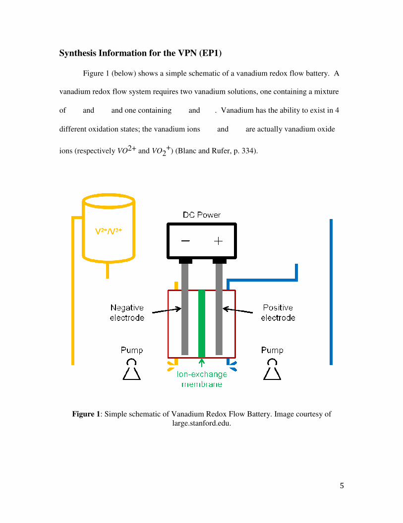
Figure 1 (below) shows a simple schematic of a vanadium redox flow battery. A

vanadium redox flow system requires two

of and and one containing

different oxidation states; the vanadium ions

ions (respectively VO2+ and

Figure 1: Simple schematic of Vanadium Redox Flow Battery.

for the VPN (EP1)

Figure 1 (below) shows a simple schematic of a vanadium redox flow battery. A

vanadium redox flow system requires two vanadium solutions, one containing a mixture

and one containing and . Vanadium has the ability to exist in 4

ifferent oxidation states; the vanadium ions and are actually vanadium oxide

and VO2+) (Blanc and Rufer, p. 334).

: Simple schematic of Vanadium Redox Flow Battery. Image courtesy of large.stanford.edu.

5

Figure 1 (below) shows a simple schematic of a vanadium redox flow battery. A

one containing a mixture

ility to exist in 4

are actually vanadium oxide

Image courtesy of

6

In essence, a vanadium redox flow battery acts an extremely large, rechargeable

battery. While electricity is being generated, the battery is charged, with the following

forward reactions taking place at the anode and cathode, respectively:

��� � �� � �� �� � � � �� � 2�� � ��

When discharging, the reverse of these two reactions takes place. As with any battery,

electric current is produced (during discharge) when electrons travel from the negative

anode to the positive cathode. In a flow battery, however, the two separate vanadium

solutions are pumped across opposite sides of an ion exchange membrane, which allows

for the flow of hydrogen ions as they are produced in either half-cell of the battery.

The design variable that this process will examine is the flow rate of vanadium

solution delivered to each cell. As the operating voltage for each cell is dependent upon

the lowest voltage across each membrane, higher flow rates will raise the voltage in areas

close to the cell output (where voltage will be lowest) by reducing the accumulation of

discharge products (��� and �� on each side of the cell membrane. Greater flow

rates, however, also require higher generation energies. Therefore, this project’s purpose

will be to determine a flow rate that optimizes power production versus the requisite

power consumption for pumping.

While power output and consumption are the primary economic drivers of a

vanadium redox flow battery, other factors, such as equipment and materials, are also

important considerations. In order to construct each cell, current collectors, carbon felt,

and a membrane permeable to protons are needed, as well as vanadium pentoxide and

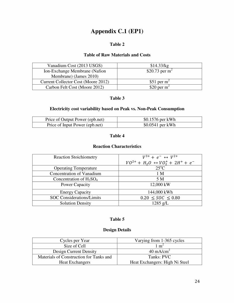
sulfuric acid, which is used to create the vanadium solutions. Table 2 (appendix C.1)

describes these costs (Moore p.241).

7

Another economic concern is the price at which power can be bought and sold.

Using the power prices from EPB Power Company’s website (www.epb.net), the price of

input power (needed to charge the battery) and output power (discharged by the battery)

seen in Table 3 (appendix C.1) were generated.

Physical characteristics of the system, such as the operating temperature and

molarity of solutions, also need to be established. Choices in materials for the heat

exchangers and tanks are similarly decided. For the tanks, PVC is used, as it represents a

cost effective material that is resistant to acid corrosion (according to the PVC supply

website www.usplastic.com). Owing to its high thermal conductivity and resistance to

corrosion, high nickel steel will be utilized for the heat exchanger (according to the steel

supply websitewww.regentsteel.net). Tables 4 and 5 (appendix C.1) delineate these

characteristics.

8

Input/Output Analysis (EP2)

Input/Output analysis is based solely upon simple algebraic equations that

describe the input and output of the system. In this case, the input is the cost of power

bought, and the output is the cost of power sold. This model allows for the maximum

profit potential, as all processing costs are ignored. Utilizing peak and off-peak power

cost rates, the power bought will be during the cheaper, off-peak periods while the power

sold will be during the more expensive peak periods, maximizing profit. The numbers

generated for the peak and off-peak rates are based upon the rates given by the EPB

Power Company, a company that provides rates comparable to those throughout the

United States. For the charging and discharging energy to be calculated, however,

electrical efficiency for the system must be calculated (see Appendix A). Once the

electrical efficiency has been calculated, the input/output profit is then compared against

a variable, in this case number of cycles of charge and discharge per year, which is

illustrated in Figure 3 (Appendix C.2). Using the assumption of 100% availability

throughout the year (all 365 possible cycles), the input/output analysis predicts a

profitability of $4,736,015.50/year (see Appendix A). Though this level of analysis does

not include many important variables, it indicates that this process has the potential to

become profitable.

9

Optimization

The design variable to be optimized in this procedure was the flow rate of the

vanadium solution across the cell membrane. In order to find this optimized flow rate, a

numerical approach was used. Utilizing the program MATLAB, this computational

approach was carried out through a computer program. Prior to the completion of the

economic potential calculation, optimization was performed due to the complexity of the

optimization of flow rate. The entire basis of prior work (Moore 2012) was performed

assuming that flow rate was so high that the state of charge did not drop across the

membrane. This was a very unrealistic assumption because of the immense amount of

friction generated within the stacks (Blanc 2010). Since friction increases by a factor of

velocity squared (equation [2]), clearly the optimal flow rate could not occur at a rate

where SOC drop is negligible.

��,� � ������

����� ��� � ���

����� [2]

The development of a model and a computer program was required to efficiently

complete the optimization. The MATLAB code (appendix E) was developed for that

reasoning. The basis of the entire model used was the assumption that the flow of

electrons across the membrane remains constant with time and flow rate. The accuracy of

this model could likely be questioned because the membrane would likely not remain

completely saturated under lower state of charges. However, due to the complexities of

modeling the reaction and diffusion near the membrane no further investigation was

made into the accuracy of the constant electron flow model. The electron flow was easily

calculated since the area and current density were both known for the membrane. The

electron flow rate was equal to the depletion of Vn2+ to Vn3+, therefore a simple balance

10

of Vanadium concentrations around the cell was used to calculate the exit state of charge

of a cell. Then using an equation derived from the Nernst Equation (equation [14])

voltage could be produced as a function of time.

� � �� � � !"# ln &'(�

)*�&'( � [14]

The program initially started with the minimum flow rate possible for developing

electricity. This flow rate would be the flow rate that would produce a state of charge of 0

out of the cell when the entering state of charge would be 0.2. This assumption was made

because the voltage produced by cell at any time is only a function of the lowest (exiting

fluid) state of charge in the cell. Thus, if the flow rate was run any lower than this

minimum flow rate, no electricity would be produced at the end of the cycle.

The program then found a tightly fitting equation to represent voltage as a

function of time. The average value of this function overall all times was then saved in an

output matrix. The flow rate was then increased by multiples of the minimum flow rate,

from a range of 1.01*fmin to 50*fmin. The average voltage at each flow rate was added

to output matrix. The power generated over the discharge cycle for each flow rate was

then generated (equation [15]).

+ � �, [15]

The next step in order to optimize the VRFB flow rate is to take into

consideration the significant head loss in the system. Essentially, the head loss can be

placed into two categories: that from the piping system and that from the cell stacks. As

the fluid-stack interface is much greater in area than that of the piping system, a vast

majority of the head loss occurs in the cell stacks. To calculate the pipe head loss, the

11

MATLAB code begins a loop that determines whether the flow is turbulent or laminar,

which then determines whether equation [3] or [4] is used as the friction factor. The loop

then continues as it combines equations [1] and [2] to calculate the piping head loss from

each given flow rate:

∆./�/0 � 12 3∆���� � ∆4 � �� � ��5 [1]

��,� � ������

����� ��� � ���

����� [2]

�� � 6780�

[3]

*

9��� 12 log < =�

�.?��� .@*

80�9��A [4]

In this case, the flow rate in the code is varied from the minimum calculated value to 50

times the minimum value. Outside of this flow rate loop, the number of cells is also

varied from 4000 to 10000, giving a large range of flow rates at various cell numbers.

Having such a unique, complicated structure, the head loss calculations incurred

because of the stacks must be found empirically. In this case, finite element method

(FEM) simulations may be run in order to generate a hydraulic resistance value, which,

combined with equation [6] yield the pressure drop due to the stacks.

∆.BCDEF � G�~ [6]

The addition of the head loss from the piping and the cell stacks then yields the total head

loss for the system, which can be substituted into equation [8] to find the power required

to pump the liquid across the total number of cells.

+/I�/ � 2�/G � ∆.G [8]

In order for the optimal flow rate to be found, the maximum difference between the

required power for pumping and the power generated by the cells must be calculated for

12

each flow rate. Once the code has accomplished this, it returns the highest difference

value found in the array of differences. These matrices of power differences can then be

used to develop plots against various values, such as number of cells or flow rate.

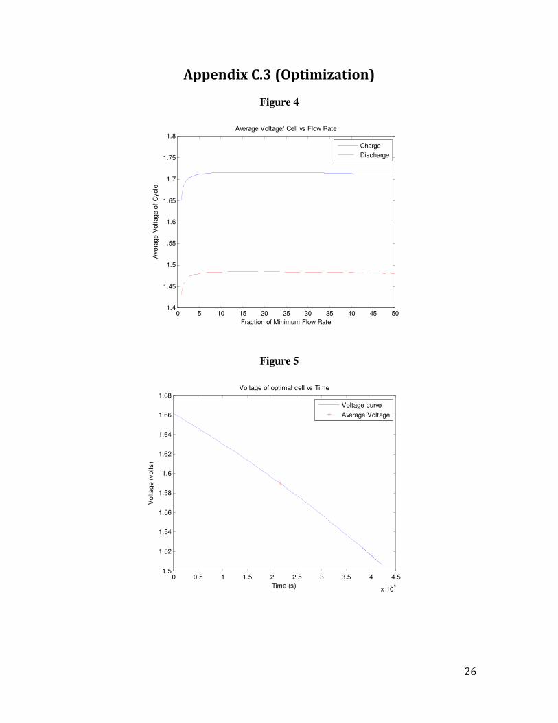
The output of the optimization program includes four figures and several design

variables. Figure 4 (appendix C.3) is developed the by the calculations of the average

voltage required to charge and discharge the cells over the various flow rates. Figure 4

demonstrates two main points. The first is that the cell efficiency being less than one

causes the battery to require more power to charge the than it can discharge. Figure 4

also demonstrates that the average voltage of the cell increases very quickly as flow rate

is increased. The average voltage quickly approaches an asymptote, thus after a large

enough flow rate was reached any gains in power generation by increasing the flow rate

would be negligible.

Figure 5 (appendix C.3) shows the voltage of the cell as a function of time at the

optimal flow rate. This voltage curve was significant because it describes the operation of

the battery. While the voltage for power generated was estimated to be the average of this

curve (denoted *), the actual power generated for this curve at any given time would be

the current produced multiplied by the number of cells multiplied by the voltage on the

curve at any given time.

Figure 6 (appendix C.3) shows the net power generated as a function of flow rate.

This graph demonstrates the main theory behind the optimization used. At some point,

the power to generate a flow rate from pumps would become greater than the power

gained by a faster flow rate. Thus the net power generation curve could be used to find

the optimal flow rate for the system. This data point was found by simply finding the k

13

which develops the maxima clearly seen in figure three. This figure was also varied over

a large variety of cell numbers to show how net power generation changed as a function

of cells.

Figure 7 (appendix C.3) shows the result of generation of figure three under a

variety of cell numbers. Figure 6 shows important data for further scale up and down of

the system. It turns out that the maximum net power (net power under optimal flow rate)

increases linearly with the number of cells in the system. An additional result of the

development of figure 6 was that the optimal flow rate was independent of the number of

cells in the system.

Finally, the program outputs several key design variables. The average voltage of

the system under optimal flow rate (see figure 5) was developed as described above. The

optimal flow rate (see figure 6) was also stated. The number of cells needed for the

system to develop the desired power (12 MW) was developed by use of the data in figure

6. The actual power generated for that exact integer was an additional output. The

number of cells in the stack was found by assuming the optimal voltage for the system to

output was 120 Volts. Thus, 120 volts was divided by the average voltage and rounded to

the nearest integer. Thus, 54 stacks of 75 cells were found to be optimal for the system.

In addition tank size was calculated (equation [23] and [ 24], appendix C.3) by the

calculation of moles of vanadium required to provide all the cells operation from 0.8

SOC to 0.2 SOC for twelve hours.

JK � ),B LB ME MB /)O PQR� 1 QR�S [23]

�C � TU(U

[24]

14

The moles of vanadium calculated were used to develop the weight of vanadium or

vanadium oxide required for the solution. Finally, the total surface was calculated by

multiplying number of cells by the surface area of membrane in each cell. Finally, the

pump power used was calculated specifically for the optimal flow rate by methods

previously used to calculated power required for the pump. Upon successfully completing

this optimization, a sound understanding of the effects of flow rate upon the VRFB

system (most importantly, increasing the head loss, cell voltage, cell power, and pump

power required) was attained. Using this newfound knowledge of the optimization in the

VRFB system, a successful economic analysis on this same system could be conducted.

15

Power Capacity Analysis (EP3)

For EP3, we considered the costs that scale with the power capacity. This includes

systems converting electricity from AC to DC, materials used to construct the cells and

structures, costing for pumps needed to run the systems. Pump costing was found using

methods described in Chemical Engineering Process Design and Economics (Ulrich

2004.) The number of stacks and cells were calculated from the optimization steps.

Power lost was then calculated using equation [16]. This lost energy was all assumed to

be lost to heat. Using equation [17], the heat generated from charge and discharge was

approximately 9 10@ YB and 8.4 10@ Y

B respectively. However a temperature increase of

only .02 degrees Celsius from equation [18], no heat exchanger or thermal system is

needed to control temperature.

MB � \�� ]� ^_

[16]

` � + )1 1 a� [17]

Δc � d (e #f

[18]

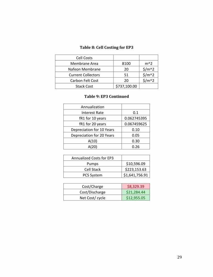
Using an interest rate of 10% and a lifespan of 10 or 20 years (stacks and pumps

were assumed to have a life of 10 years, everything else 20), the fraction of the initial

capital investment was found using equation [19] to be 0.0627 and 0.067.

�8] � gh �)ij� k)ij� klim�*

g [19]

Using both equation [20] and[ 21], the annualized cost was found to be $223,153.63 for

the cell stack. EP3 was completed by using equation [22] and found to be $2,853,088.28

for 100% runtime at 365 days/yr. All specific data can be found in Appendix C.4.

16

�� � *g [20]

nR � REoBC). 14 � �8] � �� [21]

�+� � �+ 1 nRB 1 nRpqr 1 nR/ 1 nR\(& [22]

17

Energy Capacity Analysis (EP4)

For EP4, energy capacity was taken into consideration for costing. The number of

moles of vanadium was found to be 6044000 by using equation [23], and volume of

vanadium was found using a simple conversion shown in equation [24].

JK � ),B LB ME MB /)O PQR� 1 QR�S [23]

�C � TU(U

[24]

Using the price of $14.33 (James 2010) for kg of Vanadium Oxide, the total cost of

Vanadium was found to be approximately $7.9 million. Sulfuric Acid cost about

$415,000 at $.07 per kg (Sigma Aldrich.) Tank sizing was found to be 6044 m3 with a

cost estimated around $3.2 million (Ulrich 2004.) With a cost of $8,330 per charge and a

gain of $21,000 per discharge, the net gain per cycle was around $13,000. This stayed

constant due to the fact that no more operating costs were added after EP3. Thus the

slope of the economic potential lines remained constant after EP3. The specific data

generated in EP4 can be found in appendix C.5. The results of EP4 can be found in

tabular form in appendix D.1 and in figure 8 (appendix D.2).

18

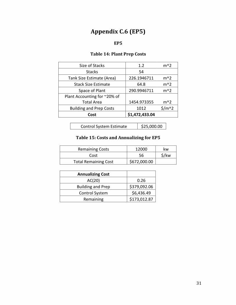
Balance of Plant Analysis (EP5)

Included in the balance of plant costs are those associated with construction and

land costs, control system costs, and building/site preparation costs. Using the number of

stacks (and their square footage), tank square footage, an estimate of the plant space is

generated (Table 14, appendix C.6). Predicting that the plant space is approximately 20%

of the total space needed, a final square footage number is also generated (Table 14,

appendix C.6). The rest of the costs are given based upon the calculated square footage

(Tables 14 and 15, appendix C.6), or based upon the numbers seen in Mark Moore’s

report on VRFB (Moore 2012). The final cost of the balance of plant analysis is found

with: �+@ � �+7 1 nsstuvw4�x Ryz{z �|y} �+@ (Moore 2012). The specific data

generated in EP5 can be found in appendix C.6. The results of EP5 can be found in

appendix D.1 (tables) and D.2 (graph).

19

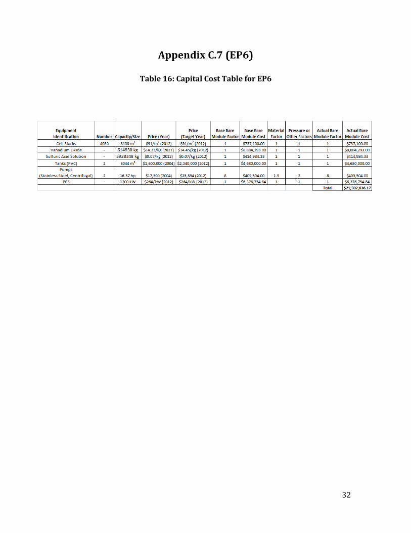
Capital Investment Analysis (EP6)

EP6 was a simple list of all capital costs calculated in EP3 through EP5. Table 17

(appendix C.7) estimates the total capital required to develop the optimized 12 MW

Vanadium Redox Flow Battery. This capital was annualized in Economic Potentials 3

through 5 and thus already included in the overall analysis of the report. The

annualization of the capital was performed based on a 10% interest rate and the

assumption that pumps and stacks would have a life of ten years while all other aspects of

the system would have a life of twenty years. However, the actual capital required for the

proposed Vanadium Redox Battery exists in table 16.

20

Conclusions

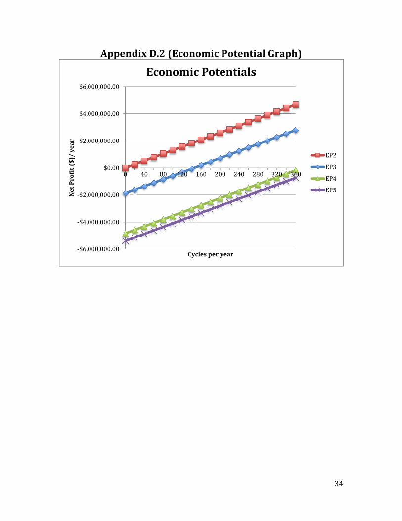
Appendix D represents the conclusions of the economic analysis. After the

inclusion of all capital costs, the 12 MW vanadium redox flow battery cannot be

recommended for economic benefit currently. The massive capital costs associated with

the project (table 16) are the major contributions to the annualized expense. Specifically

the cost of Vanadium oxide causes the project to rapidly become unfeasible. The

annualized expense of Vanadium is over $2 million. Also, the PCS equipment for power

conversion contributes to the massive capital costs with over $6 million in capital. Thus,

if the cost of these two capital expenses were lessoned then the project would likely be

feasible economically. Perhaps a used PCS system from a decommissioned power source

could provide a cheaper alternative to the massive capital of a new system. However, the

cost of vanadium shows no great alternatives. The only hope is that the cost of vanadium

will continue to decrease with time. Vanadium still currently represents essentially the

cheapest metal for use in a redox battery. However, $14.33/ kg is far from feasible

because of the over $7 million in capital this price represents. As demand for vanadium

increases across the world, additional mines could be constructed, increasing the

availability and lowering the cost. Thus, only time could help make this project feasible

due to the massive amounts of vanadium required for a 12 MW plant. In the current

scenario, though, VRFBs may become a necessary component of the grid due to the

implementation of green power sources. Thus, under the most ideal scenario with 100%

cycle availability the battery will lose $664,153.07 annually. In fact, even under the most

ideal scenario, the price of the sold electricity would need to be raised approximately

$.03/kWh (from the value of $.1576/kWh) simply to break even over the year.

21

Appendix A (Membrane efficiency)

Figure 2

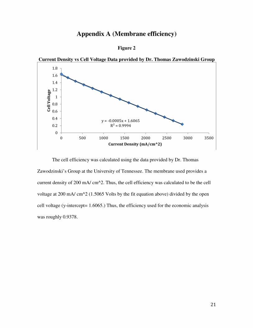
Current Density vs Cell Voltage Data provided by Dr. Thomas Zawodzinski Group

The cell efficiency was calculated using the data provided by Dr. Thomas

Zawodzinski’s Group at the University of Tennessee. The membrane used provides a

current density of 200 mA/ cm^2. Thus, the cell efficiency was calculated to be the cell

voltage at 200 mA/ cm^2 (1.5065 Volts by the fit equation above) divided by the open

cell voltage (y-intercept= 1.6065.) Thus, the efficiency used for the economic analysis

was roughly 0.9378.

y = -0.0005x + 1.6065R² = 0.9994

0

0.2

0.4

0.6

0.8

1

1.2

1.4

1.6

1.8

0 500 1000 1500 2000 2500 3000 3500

Ce

ll V

olt

ag

e

Current Density (mA/cm^2)

22

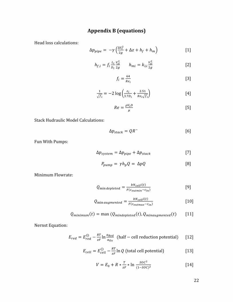
Appendix B (equations)

Head loss calculations:

∆./�/0 � 12 3∆���� � ∆4 � �� � ��5 [1]

��,� � ������

����� ��� � ���

����� [2]

�� � 6780�

[3]

*

9��� 12 log < =�

�.?��� .@*

80�9��A [4]

�� � ~���� [5]

Stack Hudraulic Model Calculations:

∆.BCDEF � G�~ [6]

Fun With Pumps:

∆.B�BC0� � ∆./�/0 � ∆.BCDEF [7]

+/I�/ � 2�/G � ∆.G [8]

Minimum Flowrate:

G��� �0/�0C0� � ��_����)C #)E�����k�E�k [9]

G��� DI��0gC0� � ��_����)C #)E����f��E�k [10]

G��g��I�){ � max )G��g�0/�0C0�){ , G��gDI��0gC0�){ [11]

Nernst Equation:

��0� � ��0�� 1 8!

"# ln D���D��

)half 1 cell reduction potential [12]

�E0�� � �E0��� 1 8!

"# ln G (total cell potential) [13]

� � �� � � !"# ln &'(�

)*�&'( � [14]

23

General Electricity Power Equation:

+ � �, [15]

Power Capacity Considerations (EP3):

MB � \�� ]� ^_

[16]

` � + )1 1 a� [17]

Δc � d (e #f

[18]

�8] � gh �)ij� k)ij� klim�*

g [19]

�� � *g [20]

nR � REoBC). 14 � �8] � �� [21]

�+� � �+ 1 nRB 1 nRpqr 1 nR/ 1 nR\(& [22]

Energy Capacity Analysis (EP4):

JK � ),B LB ME MB /)O PQR� 1 QR�S [23]

�C � TU(U

[24]

�+7 � �+� 1 nR� 1 nR! 1 nRp&'7 [25]

24

Appendix C.1 (EP1)

Table 2

Table of Raw Materials and Costs

Vanadium Cost (2013 USGS) $14.33/kg

Ion-Exchange Membrane (Nafion Membrane) (James 2010)

$20.73 per m2

Current Collector Cost (Moore 2012) $51 per m2

Carbon Felt Cost (Moore 2012) $20 per m2

Table 3

Electricity cost variability based on Peak vs. Non-Peak Consumption

Price of Output Power (epb.net) $0.1576 per kWh

Price of Input Power (epb.net) $0.0541 per kWh

Table 4

Reaction Characteristics

Reaction Stoichiometry ��� � �� � ��

�� � � � �� � 2�� � �� Operating Temperature 25oC

Concentration of Vanadium 1 M

Concentration of H2SO4 5 M

Power Capacity 12,000 kW

Energy Capacity 144,000 kWh

SOC Considerations/Limits 0.20 ¡ QR ¡ 0.80 Solution Density 1285 g/L

Table 5

Design Details

Cycles per Year Varying from 1-365 cycles

Size of Cell 1 m2

Design Current Density 40 mA/cm2

Materials of Construction for Tanks and Heat Exchangers

Tanks: PVC Heat Exchangers: High Ni Steel

Net profit versus cycles per year

$0.00

$2,000,000.00

$4,000,000.00

$6,000,000.00

0

Ne

t P

rofi

t ($

)/ y

ea

r Net Profit vs. Cycles per Year

Appendix C.2 (EP2)

Figure 3

Net profit versus cycles per year

100 200 300

Cycles per year

Net Profit vs. Cycles per Year

25

26

Appendix C.3 (Optimization)

Figure 4

Figure 5

0 5 10 15 20 25 30 35 40 45 501.4

1.45

1.5

1.55

1.6

1.65

1.7

1.75

1.8Average Voltage/ Cell vs Flow Rate

Fraction of Minimum Flow Rate

Avera

ge V

oltage o

f C

ycle

Charge

Discharge

0 0.5 1 1.5 2 2.5 3 3.5 4 4.5

x 104

1.5

1.52

1.54

1.56

1.58

1.6

1.62

1.64

1.66

1.68Voltage of optimal cell vs Time

Time (s)

Voltage (

volts)

Voltage curve

Average Voltage

27

Figure 6

Figure 7

0 5 10 15 20 25 30 35 40 45 502.84

2.86

2.88

2.9

2.92

2.94

2.96

2.98x 10

7 Net Power Generated vs. Flow Rate

Multiple of Minimum Flow Rate

Net

Pow

er

Genera

ted (

W)

4000 5000 6000 7000 8000 9000 100001

1.2

1.4

1.6

1.8

2

2.2

2.4

2.6

2.8

3x 10

7

Number of Cells

Maxim

um

Net

Pow

er

(W)

Max Net Power vs. Number of Cells

28

Appendix C.4 (EP3)

Table 6: Heat Calculations for EP3

Number of Cells 4050

Flow Rate 1.1142 L/s cell

Flow Rate 4.51251 m^3/s

Density of Water 1000000 g/m^3

Mass Flow Rate 4512510 g/s

Membrane Efficiency 0.93

Heat Capacity 4.2 J/g*k

Power Generated 12000000 W

Heat from Charge 903225.81 J/s

Heat from Discharge 840000 J/s

Delta T Charge 0.02 C

Delta T Discharge 0.02 C

Table 6: Pump Costing for EP3

Pump Size 12358 W

Pump Size (hp) 16.57 hp

Pump Cost/Pump 17500

Pump Efficiency 0.75

Electricity/Charge (Discharge

already accounted for) 197.728 kwh

Annualized Electricity

Cost/Pump 10.16519648

Number of Pumps 2

Capital of Pumps $35,000.00

Annualized running cost/cycle $20.33

Table 7: PCS equipment costing for EP3

PCS Equipment Costs 265 $/kw

Discharge Power 11160 kw

Charge Power 12903.23 kw

PCS Charge (AC-> DC) $2,957,400.00

PCS Discharge (DC -> AC) $3,419,354.84

29

Table 8: Cell Costing for EP3

Cell Costs

Membrane Area 8100 m^2

Nafeon Membrane 20 $/m^2

Current Collectors 51 $/m^2

Carbon Felt Cost 20 $/m^2

Stack Cost $737,100.00

Table 9: EP3 Continued

Annualization

Interest Rate 0.1

fR1 for 10 years 0.062745395

fR1 for 20 years 0.067459625

Depreciation for 10 Years 0.10

Depreciation for 20 Years 0.05

A(10) 0.30

A(20) 0.26

Annualized Costs for EP3

Pumps $10,596.09

Cell Stack $223,153.63

PCS System $1,641,756.91

Cost/Charge $8,329.39

Cost/Discharge $21,284.44

Net Cost/ cycle $12,955.05

30

Appendix C.5 (EP4)

Table 10: Vanadium Calculations

Vanadium Needed 6044000 mols

Vanadium Oxide

Needed 549680 kg

Cost of Vanadium

Oxide 14.33 $/kg

Total Cost of

Vanadium $7,876,914.40

Table 11: Sulfuric Acid Calculations

Sulfuric Acid Needed 5928347.52 kg

Cost of Sulfuric Acid 0.07 $/kg

Total Cost of H2SO4 $414,984.33

Table 12: Tank Sizing

Tanks Needed 2

Tank Size 6044.4 m^3

Cost of Tank $1,600,000.00

Cost of Tanks $3,200,000.00

Table 13: Annualization and EP4

A(20) 0.26

Vanadium $2,027,987.43

Sulfuric Acid $106,841.71

Tanks $823,870.80

EP4

Cost/Charge $8,329.39

Cost/Discharge $21,284.44

Net cost/Cycle $12,955.05

31

Appendix C.6 (EP5)

EP5

Table 14: Plant Prep Costs

Size of Stacks 1.2 m^2

Stacks 54

Tank Size Estimate (Area) 226.1946711 m^2

Stack Size Estimate 64.8 m^2

Space of Plant 290.9946711 m^2

Plant Accounting for ~20% of

Total Area 1454.973355 m^2

Building and Prep Costs 1012 $/m^2

Cost $1,472,433.04

Control System Estimate $25,000.00

Table 15: Costs and Annualizing for EP5

Remaining Costs 12000 kw

Cost 56 $/kw

Total Remaining Cost $672,000.00

Annualizing Cost

AC(20) 0.26

Building and Prep $379,092.06

Control System $6,436.49

Remaining $173,012.87

32

Appendix C.7 (EP6)

Table 16: Capital Cost Table for EP6

33

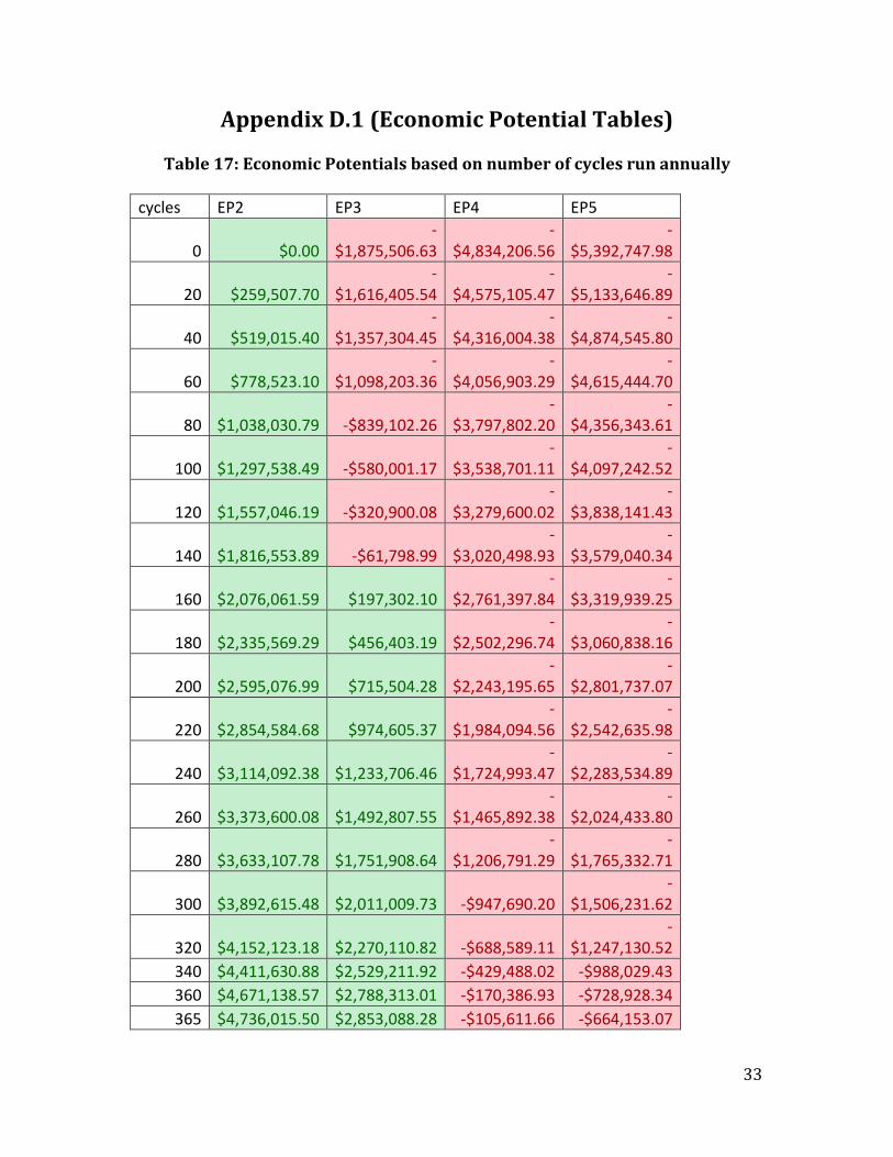
Appendix D.1 (Economic Potential Tables)

Table 17: Economic Potentials based on number of cycles run annually

cycles EP2 EP3 EP4 EP5

0 $0.00

-

$1,875,506.63

-

$4,834,206.56

-

$5,392,747.98

20 $259,507.70

-

$1,616,405.54

-

$4,575,105.47

-

$5,133,646.89

40 $519,015.40

-

$1,357,304.45

-

$4,316,004.38

-

$4,874,545.80

60 $778,523.10

-

$1,098,203.36

-

$4,056,903.29

-

$4,615,444.70

80 $1,038,030.79 -$839,102.26

-

$3,797,802.20

-

$4,356,343.61

100 $1,297,538.49 -$580,001.17

-

$3,538,701.11

-

$4,097,242.52

120 $1,557,046.19 -$320,900.08

-

$3,279,600.02

-

$3,838,141.43

140 $1,816,553.89 -$61,798.99

-

$3,020,498.93

-

$3,579,040.34

160 $2,076,061.59 $197,302.10

-

$2,761,397.84

-

$3,319,939.25

180 $2,335,569.29 $456,403.19

-

$2,502,296.74

-

$3,060,838.16

200 $2,595,076.99 $715,504.28

-

$2,243,195.65

-

$2,801,737.07

220 $2,854,584.68 $974,605.37

-

$1,984,094.56

-

$2,542,635.98

240 $3,114,092.38 $1,233,706.46

-

$1,724,993.47

-

$2,283,534.89

260 $3,373,600.08 $1,492,807.55

-

$1,465,892.38

-

$2,024,433.80

280 $3,633,107.78 $1,751,908.64

-

$1,206,791.29

-

$1,765,332.71

300 $3,892,615.48 $2,011,009.73 -$947,690.20

-

$1,506,231.62

320 $4,152,123.18 $2,270,110.82 -$688,589.11

-

$1,247,130.52

340 $4,411,630.88 $2,529,211.92 -$429,488.02 -$988,029.43

360 $4,671,138.57 $2,788,313.01 -$170,386.93 -$728,928.34

365 $4,736,015.50 $2,853,088.28 -$105,611.66 -$664,153.07

Appendix D.2 (Economic Potential Graph)

-$6,000,000.00

-$4,000,000.00

-$2,000,000.00

$0.00

$2,000,000.00

$4,000,000.00

$6,000,000.00

0 40

Ne

t P

rofi

t ($

)/ y

ea

rEconomic Potentials

Appendix D.2 (Economic Potential Graph)

80 120 160 200 240 280 320 360

Cycles per year

Economic Potentials

34

Appendix D.2 (Economic Potential Graph)

360

EP2

EP3

EP4

EP5

35

Appendix E (Matlab Optimization Code) clc clear all close all

% The following code was written for the optimization of a vanadium redox % flow battery. Specifically the flow rate through the battery was % optimized by finding the maximum point of net power generated by the % battery during discharge taking into account the cost of power for % pumping the solution through the membrane. This code was generated by % Kevin Spellman, Kendrick Stiles, and Ian Little for the purpose of Senior % Design project for CBE 488 and subsequent Honor's Thesis. The code may % not be reused by others without premission of the authors and proper % recognition. All data generated by the code is also property of the % authors and proper recognition is necessary for its use. soc0=0.8; socf=0.2; concV = 1; %Conc of Vanadium Vn20=soc0.*concV; %Vn2+ + Vn3+ = 1 molar always by definition Vn2f=socf.*concV; cd=.2; %A/cm^2 Area=10000; %cm^2 current=Area.*cd; %amps= coloumbs/ s F= 96485.3365; %Coloumbs/ mol eflow=current./F; %mol/s t=0:15*60:12*3600; %min measuring every 15 minutes flowmin=eflow/0.2; %lowest possible SOCin=0.2/ SOCout=0 %derived from mass balance flowminm3 = flowmin*.001; %min flow in m^3/s vavg=[]; k =[]; psi = [];

for kk=1:5000 %percentage of minimum flow rate used in trial k(kk)=kk*.01; if k(kk)<1; k(kk)=1; end psi(kk)=k(kk).*flowmin; %psi= flowrate (L/s) ilast=length(t); tspc=t(ilast).*eflow./(Vn20-Vn2f); t(ilast)=t(ilast)-1; Vn2out=[]; Vn2in=[]; SOC=[];

for i=1:ilast Vn2in(i)= (Vn20.*tspc-eflow.*t(i))./tspc; Vn2out(i)=(Vn2in(i).*psi(kk)-eflow)./(psi(kk)); SOC(i)=Vn2out(i)./1 ; %1 molar solution end E0=1.602; %open circuit voltage= 1.602 R=8.314; %J/mol K Temp=298; %Assume STP V=E0+R.*Temp./F.*log(SOC.^2./(1-SOC).^2);

% plot(t,V); % hold p=polyfit(t,V,2); f=polyval(p,t);

36

% plot(t,f); vavg(kk)=mean(f); end n=0.93; Vdischarge=vavg.*n; Vcharge=vavg./n;

gpm = psi*15.85; %Conversion of flow into gpm (1 L/s = 15.85 gpm) m3 = psi*.001; %Conversion of flow into m^3/s (1 L/s = .001 m^3/s)

% figure(1) % plot(k,Vcharge) % hold on % plot(k,Vdischarge,'--r') % title('Average Voltage/ Cell vs Flow Rate') % xlabel('Fraction of Minimum Flow Rate') % ylabel('Average Voltage of Cycle') % legend('Charge','Discharge')

pcharge=Vcharge.*current; pdischarged=Vdischarge.*current;

% figure(2) % plot(k,pcharge) % hold on % plot(k,pdischarged,'--r') % title('Power genererated/ Cell vs Flow rate') % xlabel('Fraction of Minimum Flow Rate') % ylabel('Power per cell (W)') % legend('Power to charge', 'Power to discharge')

Powergen=12*10^6; %W Ncells= Powergen./pdischarged;

% figure(3) % plot(k,Ncells); % title('Number of cells vs flow rate') % xlabel('Fraction of Minimum Flow Rate') % ylabel('Number of cells')

%% Head loss/Velocity calcs

htotal = []; %Total head loss di = .1; %Diameter (m) A1 = pi*(di/2)^2; %Pipe area (m^2) vel = []; llength = 1; %Pipe length (m) gamma = -1; %DeltaP equation constant gravity = 9.81; %Acceleration due to gravity (m^2/s) density = 997; %Density of solution at STP (kg/m^3) viscosity = 0.9; %Viscosity of solution at STP ( elbow = 2; %Number of 90 degree elbows kelbow = 1.5; %Constant for head loss due to elbows dZ = 10; %Change in height (m) Ratio = 14186843/19; %Stack flow resistance (Pa/m^3)/# of cells Ppump = [];

37

Pdiff = []; peff=0.75 %assuming 75% pump efficiency

vel = m3/A1; %Calculates fluid velocities depending on pipe size powermaxes = []; %Matrix that will be filled with max net power outputs newcells = [4000:50:10000]; %Matrix of cell numbers to use flowmaxes = []; %Matrix with maximum flow rates from each cell number kopts = []; pwrmx = [];

for dd = 1:numel(newcells)

for ii = 1:kk %Calculates head losses for each velocity

Re = density*di*vel(ii)/viscosity; %Reynolds #

if Re < 2100 %Calc for friction factor based on Re fi=65./Re; else fi0=65./Re; eata=1; %go back to find out roughness fi=fi0; limit=.001./100; i3=1; i5=1; fi2=[]; fi2(i5)=fi0; while i3>limit i5=i5+1; fi2(i5)=(1./(-2.*log(eata./(3.7.*di)+2.51./(Re.*sqrt(fi2(i5-1))))))^2; i3=abs(fi2(i5)-fi2(i5-1))./fi2(i5); fi=fi2(i5); end end

hfi = fi*llength/di*vel(ii)^2/(2*gravity); %Head loss from length hm1 = elbow*kelbow*vel(ii)^2/(2*gravity); %Head loss from elbows htotal = hm1+hfi;

dPpipe = -1*gamma*(vel(ii)^2/(2*gravity)+dZ+htotal); %Calc dP for pipe R = Ratio*newcells(dd); %Calc resistance of flow with actual number of %cells dPstack = m3(ii)*R; %Calc dP for stack dPtotal = dPpipe + dPstack; %Total dP Ppump(ii) = dPtotal*m3(ii)./peff; %Power used by pump Pdiff(ii) = pdischarged(ii)*newcells(dd) - 2.*Ppump(ii); %Power %difference between pumping power and power discharged

end

figure(4) plot(k,Pdiff) title('Net Power Generated vs. Flow Rate') xlabel('Multiple of Minimum Flow Rate') ylabel('Net Power Generated (W)')

38

for ii = 2:kk

if Pdiff(ii) > Pdiff(ii-1)

flowmax = m3(ii); %Flow rate at which power diff is maximum Pmax = Pdiff(ii); %Maximum power difference i7=ii; end end

flowmaxes(dd) = flowmax; kopts(dd) = flowmax./flowminm3; powermaxes(dd) = max(Pdiff); pwrmx(dd) = Pmax;

end

figure(5) plot(newcells,powermaxes) xlabel('Number of Cells') ylabel('Maximum Net Power (W)') title('Max Net Power vs. Number of Cells')

kopt=kopts(1);

% Redeveloping figures 1-3 used earlier now for optimal flow rate

psi2=kopt.*flowmin; %psi= flowrate (L/s) ilast=length(t); tspc=t(ilast).*eflow./(Vn20-Vn2f); t(ilast)=t(ilast)-1; Vn2outopt=[]; Vn2inopt=[]; SOCopt=[];

for i=1:ilast Vn2inopt(i)= (Vn20.*tspc-eflow.*t(i))./tspc; Vn2outopt(i)=(Vn2inopt(i).*psi2-eflow)./(psi2); SOCopt(i)=Vn2outopt(i)./1 ; %1 molar solution end E0=1.602; %open circuit voltage= 1.602 R=8.314; %J/mol K Temp=298; %Assume STP V=E0+R.*Temp./F.*log(SOCopt.^2./(1-SOCopt).^2);

% plot(t,V); % hold p=polyfit(t,V,2); f=polyval(p,t); figure(2) plot(t,f); title('Voltage of optimal cell vs Time') xlabel('Time (s)') ylabel('Voltage (volts)') vavgopt=mean(f); hold on tavg=0; for i7=1:length(t)

39

if V(i7)> vavgopt tavg=t(i7); i8=i7; end end plot(tavg,V(i8),'*r') legend('Voltage curve','Average Voltage')

n=0.93; Vdischargeopt=vavgopt.*n; Vchargeopt=vavgopt./n;

figure(1) plot(k,Vcharge) hold on plot(k,Vdischarge,'--r') title('Average Voltage/ Cell vs Flow Rate') xlabel('Fraction of Minimum Flow Rate') ylabel('Average Voltage of Cycle') legend('Charge','Discharge')

vavgopt kopt psi2 cellnum=0; for i9=1:numel(newcells) if powermaxes(i9) <1.2*10^7 cellnum=i9; end end cellsneeded=newcells(cellnum+1) Powergenerated=powermaxes(cellnum+1) cellsinstack=floor(120./vavgopt) stacks=cellsneeded./cellsinstack

% Calculating vanadium needed Vmols=eflow.*12.*3600./0.6.*cellsneeded;%(mols) %1/1 electron rate vs VN depletion and only 60% of vanadium is used in % depletion cycle Tanksize=Vmols./concV % Liters VnMW=50.9415; % g/mol %molecular mass of vanadium kgV=Vmols.*2.*VnMW./1000 %kg of Vneeded kgVn2O5=Vmols./2.*181.88./1000 %kg of Vn2O5 needed for solution

% Calculating Nafeon membrane size Totalsurface=Area./100^2.*2.*cellsneeded %m^2 %membrane area * cells * 2 membrances/ cell

% Sizing pump ii=round(kopt./0.01);

Re = density*di*vel(ii)/viscosity; %Reynolds #

if Re < 2100 %Calc for friction factor based on Re fi=65./Re; else fi0=65./Re; eata=1; %go back to find out roughness

40

fi=fi0; limit=.001./100; i3=1; i5=1; fi2=[]; fi2(i5)=fi0; while i3>limit i5=i5+1; fi2(i5)=(1./(-2.*log(eata./(3.7.*di)+2.51./(Re.*sqrt(fi2(i5-1))))))^2; i3=abs(fi2(i5)-fi2(i5-1))./fi2(i5); fi=fi2(i5); end end

hfi = fi*llength/di*vel(ii)^2/(2*gravity); %Head loss from length hm1 = elbow*kelbow*vel(ii)^2/(2*gravity); %Head loss from elbows htotal = hm1+hfi;

dPpipe = -1*gamma*(vel(ii)^2/(2*gravity)+dZ+htotal); %Calc dP for pipe R = Ratio*newcells(dd); %Calc resistance of flow with actual number of %cells dPstack = m3(ii)*R; %Calc dP for stack dPtotal = dPpipe + dPstack; %Total dP Pumppower = dPtotal*m3(ii)./peff%Watts %Power used by pump

41

References

Christian Blanc and Alfred Rufer (2010). Understanding the Vanadium Redox Flow

Batteries, Paths to Sustainable Energy, Dr Artie Ng (Ed.), ISBN: 978-953-307-

401-6, InTech, Available from: http://www.intechopen.com/books/paths-to-

sustainable-energy/understanding-the-vanadium-redox-flow- batteries

Eckroad, S., “Vanadium Redox Flow Batteries: An In-Depth Analysis”. Palo Alto: EPRI,

2007.

EPRI-DOE Handbook of Energy Storage for Transmission &Distribution Applications,

EPRI, Palo Alto, CA, and the U.S. Department of Energy, Washington, DC: 2003.

1001834.

James, Kalinoski, Baum. “Mass Production Cost Estimation for the Direct H2 PEM Fuel

Cell System for Automotive Applications: 2010 Update”. Directed Technologies,

Inc., Arlington, Va. (Prepared under subcontract AGB-0-40628-01 to U.S.

Department of Energy) (September 30, 2010).

Moore, Mark, Counce, Robert, et al. “A Step by Step Methodology for a Base Case

Vanadium Redox-Flow Battery”. University of Tennessee, Knoxville. 2012.

Print.

42

Mouron, Elizabeth Hope, "The Economic Potential of the All-Vanadium Redox Flow

Battery With a Focus on State of Charge" (2011). University of Tennessee Honors

Thesis Projects.

http://trace.tennessee.edu/utk_chanhonoproj/1421

Ulrich, Gail, Vasudevan, P. T. Chemical Engineering Process Design and Economics. A

Practical Guide. Second Edition. Durham , New Hampshire: Process Publishing,

2004.

Watt-Smith, M.J., Ridley, P., Wills, R.G.A., Shah, A.A. and Walsh, F.C. (2013), The

importance of key operational variables and electrolyte monitoring to the

performance of an all vanadium redox flow battery. J. Chem. Technol.

Biotechnol., 88: 126–138. doi: 10.1002/jctb.3870