142
Economic Review December 2017

Natio
nal B
ank o
f Belg
ium
Eco
no
mic R
eview
Decem
ber 2017
Economic ReviewDecember 2017

© National Bank of Belgium
All rights reserved.Reproduction of all or part of this publication for educational and non‑commercial purposes is permitted provided that the source is acknowledged.
ISSN 1780 ‑ 664X

Economic ReviewDecember 2017

5December 2017 ❙ Contents ❙
Contents
ECONOMIC PROJECTIONS FOR BELGIUM – AUTUMN 2017 7
ARE BANK LOANS BEING GRANTED TO THE BEST-PERFORMING FIRMS ? 29
THE NEGATIVE INTEREST RATE POLICY IN THE EURO AREA AND THE SUPPLY OF BANK LOANS 43
TOWARDS A NEW POLICY MIX IN THE EURO AREA ? 63
UP OR OUT ? PORTRAIT OF YOUNG HIGH‑GROWTH FIRMS IN BELGIUM 93
RECENT DEVELOPMENTS IN THE FINANCIAL SITUATION OF FIRMS 115
ABSTRACTS FROM THE WORKING PAPERS SERIES 143
CONVENTIONAL SIGNS 145
LIST OF ABBREVIATIONS 147

7December 2017 ❙ EcoNomIc pRojEctIoNS foR BElgIum – AutumN 2017 ❙
Economic projections for Belgium – Autumn 2017
Introduction
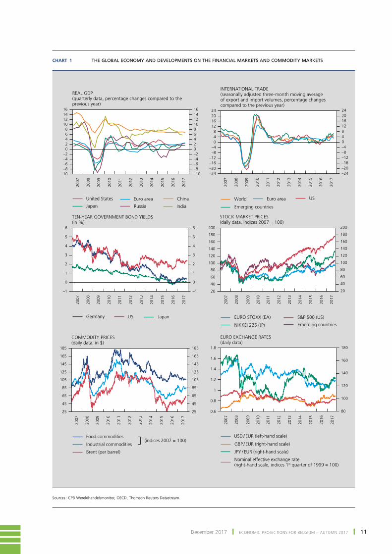
As expected, the global economy recorded relatively sus‑tained growth in the first two quarters of 2017. According to the initial quarterly statistics and the leading indicators for some major countries, this growth pace would – at least – have been maintained in the second half of the year. In the common assumptions adopted for these projections with a cut-off date of 23 November 2017, the main ones being described in box 1, it is assumed that global year-on-year growth excluding the euro area will pick up slightly at first, but then subside a little from 2018. That contraction is likely to occur because the gradual slowdown in some advanced countries will not be entirely offset by the stronger growth seen in a number of emerging countries, such as the expected strengthening of the Brazilian economic recovery.
World trade rebounded strongly in the first half of 2017 : according to the initial available data, global trade flows expanded at almost twice the pace of global GDP. This widespread phenomenon seems to be due in particular to the revival of highly import‑intensive investment. the effect of the recovery in the emerging countries combined with the increasing supply constraints in a number of advanced countries may have also sparked a further extension of the global production chains. the marked expansion of trade also makes global growth more robust and less dependent on the situation in certain individual countries. However, similar to the latest projections by other international institutions, the common assumptions used for these Eurosystem estimates consider this to be partly the result of a series of one‑off factors, and they therefore allow for a gradual decline in the trade intensity of growth during the projection period, so that the expansion of trade will fall back into line with world GDP
growth. The underlying idea is that some factors which have accentuated that trade intensity in the past, such as the progressive liberalisation of trade, will exert less influence in the future. In recent months, the financial markets have remained calm. Up to now, the tightening of monetary policy initiated in the united States and the announcement of the reduction of quantitative easing in the euro area from January 2018, as well as the ever-present geopolitical risks, have generated surprisingly little volatility. In fact, stock markets have continued rising strongly, reflecting the favourable profit outlook but probably also investors’ search for yield which is fuelling a marked increase in the prices of other assets such as property. In the euro area, interest rates are still close to their historical floor, notably on account of inflation which has risen only modestly so far. However, oil prices have staged a fairly substantial rise since mid-2017. In view of the continuation of the current production restrictions and the only temporary impact of extreme weather phenomena which mainly affected American production, that rise essentially reflects the revival of world demand for oil, driven by the favourable global economic situation. However, the most significant development occurred on the foreign exchange markets, where the euro has appreciated considerably since the summer, partly as a result of the relative adjustment of the growth figures (or outlook) for the euro area.
According to the latest statistics, the pace of activity in the euro area continued to strengthen significantly from the autumn of 2016, at an average of 0.6 % over the past four quarters. Real GDP growth is therefore estimated at 2.4 % this year, representing the strongest rise for ten years. Growth gained steam in both Germany and France, and remained very robust in Spain and the Netherlands. Recently, also Italian activity gained some momentum,

8 ❙ EcoNomIc pRojEctIoNS foR BElgIum – AutumN 2017 ❙ NBB Economic Review
even though its expansion is still clearly below the euro area average. the most relevant short‑term indicators, such as those concerning business confidence, continue to point to a very favourable outlook for the euro area in the immediate future, with growth expected to re‑main practically unchanged in the final quarter of 2017. However, according to the new Eurosystem estimates, which run until 2020 this time – and incorporate the au‑tumn projections discussed in this article and completed on 30 November – activity in the euro area is subsequently set to slow down gradually. The slowdown is due to the weakening momentum of global growth and world trade mentioned earlier, which will cause a gradual slackening of external demand, but also due to the labour market supply constraints which will be an impediment to growth in some major countries. Annual growth in the euro area is in fact predicted to slow gradually to 1.7 % by 2020. Inflation in the euro area is bolstered this year by rising energy prices. leaving aside that component and other volatile factors, core inflation is set to increase through‑out the projection period, reflecting the growing pressure of domestic costs, but will remain below 2 % at the end of 2020.
In regard to Belgium, the macroeconomic estimates were barely revised compared to the spring projections. the growth estimate for 2017 has been upgraded slightly to 1.7 %, mainly on account of the revision of the quarterly statistics for the first half of the year. However, growth will then decline gradually up to 2020, the principal factor being the moderation in the business investment cycle and the traditional drop in local government invest‑ment following the elections. The negative growth gap between Belgium and the euro area, which opened up in 2015, will diminish, but will not entirely vanish during the projection period.
In 2017, employment clearly exceeded the spring projec‑tions, partly as a result of the revision of the initial quar‑terly statistics, and actually strengthened in comparison with 2016. This implies that the expansion of employment has practically kept pace with the growth of activity for two years now, which is very unusual in the context of a cyclical upturn. Hence, there is little doubt that the job creation was driven by the recent policy measures, and especially the wage cost moderation which makes labour relatively cheaper, as well as by certain structural labour market reforms which are boosting the effective labour supply. The strong jobs growth is accompanied by a rising participation rate, particularly among older workers who are remaining active on the labour market for longer as a result of the various reforms. Yet the current forecasts still assume that the additional stimulus of those measures will fade away and that employment growth will gradually
slow down, not only because labour costs begin rising again but also owing to the increasing impact of labour market shortages – as is already evident from the grow‑ing number of unfilled vacancies – so that firms will find it increasingly difficult to obtain suitable staff. The unem‑ployment rate is set to decline further to just under 7 %, which is close to the level prevailing immediately before the great recession.
Inflation, which stands at 2.2 % in 2017, will ease con‑siderably in 2018, dropping to around 1.6 %. It will be tempered by various factors, particularly the expected levelling out of oil prices and the impact of the euro’s recent appreciation, which makes imports cheaper, but also the abolition of the energy levy on domestic electric‑ity consumption in the Flemish Region with effect from 1 January 2018. Core inflation edges upwards during the projection period even though, as in the past, the strong rise in labour costs will not be entirely passed on in prices ; instead, it will lead to moderation of profit margins.
Finally, turning to public finances, the budget deficit fell much more steeply than expected in 2017, to 1.2 % of gDp. the main factor here is the substantial increase in advance payments by companies and, to a lesser extent, the favourable effect of the strong job creation on public revenues and expenditure. However, the budget deficit is set to rise again in the years ahead, as the deterioration in the primary surplus will be only partly offset by the further fall in interest charges. At the end of the projec‑tion period, the budget deficit will still stand at 1.5 %, which is far short of the target of a structurally balanced budget. the government’s debt ratio is gradually falling, but the debt level will still exceed GDP at the end of the projection period. Here it should be remembered that, in accordance with the Eurosystem rules for such projection exercises, account is only taken of measures which, on the cut‑off date for the estimates, the government has already specified in sufficient detail and formally approved or is very likely to approve. furthermore, the estimates of the impact on the budget of certain measures, such as those to combat fraud, differ from the amounts included in the budget.
1. International environment and assumptions
1.1 World economy
After picking up in the second half of 2016, global eco‑nomic growth continued to gain momentum in 2017. Growth also became more broadly based in geographical

9December 2017 ❙ EcoNomIc pRojEctIoNS foR BElgIum – AutumN 2017 ❙
terms, in both the advanced and the emerging economies. In the advanced economies, the vigorous activity was sup‑ported by the continuing accommodative monetary policy and restoring consumer and business confidence. It was based primarily on the dynamism of domestic demand and, more particularly, on a strong investment revival. In the emerging economies, growth recorded a slightly more moderate strengthening, but the variations between countries diminished considerably. the improvement in the global macroeconomic outlook was accompanied by a world trade revival and a strong rise in the valuation of assets on global markets. conversely, commodity prices were more volatile.
In the emerging countries, there was a further slight strengthening of the robust growth of the Chinese econ‑omy. Economic activity benefited from substantial export growth which more than offset the slight slackening of domestic demand. Private consumption was fairly stable, while investment was down slightly, so that a consider‑able amount of production capacity remained unused. Fiscal policy was still relatively expansionary, and that was reflected in particular in a high level of public investment. the people’s Bank of china maintained a “neutral” mon‑etary policy stance. However, against the backdrop of a heavy debt burden and increased risks to financial stabil‑ity, the Chinese authorities took new measures to halt the constant credit expansion.
In the commodity‑exporting countries – and more espe‑cially those producing fossil fuels – activity was still de‑pressed overall by the persistently low commodity prices, although those did exceed the 2016 average. However, Brazil and Russia recorded positive growth again after two years of deep recession. In Brazil, the recovery was initially supported by agriculture, but subsequently strengthened and spread to the other economic sectors, while falling inflation bolstered household consumption. In Russia, the economy picked up gradually from the end of 2016 as a result of rising oil prices, stabilisation of the rouble, and the steady decline in inflation. Both private consumption and private investment contributed to the revival in the context of a clear restoration of confidence and improv‑ing financing conditions. Conversely, in India, the effects of the measures to rein in the shadow economy, such as demonetisation and the harmonisation of taxes on goods and services, dampened growth, which is estimated at just under 7 % this year.
As regards the advanced economies, activity in the united States surged in 2017, further fuelling the ongoing improvement in the labour market. underpinned by a marked increase in investment, growth gradually picked up, reaching 3.3 % year-on-year in the third quarter. In
November, as a result of job creation, the unemploy‑ment rate was back down to the level prevailing in the early 2000s, at 4.1 %. Private consumption remained robust, supported in particular by the wealth effects as‑sociated with the good performance of the asset markets and the rise in wages, albeit still moderate. Despite these favourable developments, inflation remained below target and inflation expectations were still relatively low.
In japan, economic activity accelerated against the back‑drop of highly accommodative financing conditions and significant government measures to support the economy. The growth of exports resulting from the upturn in inter‑national trade supported investment, while consumption benefited from a new improvement in employment. However, with energy and food prices excluded, inflation still remained close to zero. the main explanatory factor seems to be the extreme caution displayed by japanese firms in setting wages and prices. Despite unemployment running at less than 3 %, a growing labour shortage and a surge in corporate profits, wages hardly increased at all in real terms.
In the United Kingdom, the economy began to slow down at the end of 2016, after the initial resilience following the vote on 23 June 2016 in favour of exit from the European Union. Corporate investment remained modest owing to uncertainty over the decision to leave the European union, and private consumption suffered in particular from the fall in purchasing power. That fall is due more specifically to the strong rise in inflation resulting from the sharp depreciation of the pound sterling during 2016. Conversely, the lower pound boosted exports which, in contrast to imports, increased strongly. As a result, the growth slowdown was modest, and thanks to the sus‑tained job creation unemployment declined further to less than 4.5 %.
In the euro area, economic growth picked up in 2017. It was supported primarily by domestic demand and be‑came widespread across countries and sectors. Although private consumption was restrained by weak wage growth, it benefited from a new labour market revival, with the overall unemployment rate falling to 8.8 % in October, its lowest level in nine years. Investment gained support from the continuing favourable financing conditions and from the rise in consumer confidence, increased profitability and a strengthening of global demand. Exports recorded substantial growth in view of the world trade revival. The marked improvement in the macroeconomic outlook for the euro area was backed by the progress achieved in cleaning up banks’ balance sheets, although substantial outstanding amounts of non‑performing loans persist in places.

10 ❙ EcoNomIc pRojEctIoNS foR BElgIum – AutumN 2017 ❙ NBB Economic Review
Despite continuing significant discrepancies, all euro area countries contributed to the economic expansion record‑ed in 2017. While economic growth was consolidated in germany and the Netherlands, it gathered pace in france and Italy. In Spain, activity remained robust and gDp sur‑passed its pre‑crisis level.
After reaching 1.9 % in April, mainly as a result of the rise in energy prices, headline inflation in the euro area subsided again. At 1.5 % in November, it was well short of the ECB’s target of close to 2 %. Core inflation, i.e. excluding food and energy prices, increased for a time during the year to reach 1.2 % in April and in the sum‑mer. However, recently it has fallen again to just 0.9 % in November as a result of the continuing weak pricing and wage-setting dynamics.
After a marked slowdown in 2016, global trade flows recovered from the last quarter of 2016. Once again, the growth of world trade significantly outpaced the expan‑sion of activity. The stronger trade dynamics were seen in both the advanced and the emerging economies, pointing to a rise in global demand, and more particularly increased investment which has a relatively high import content. Apart from the renewed dynamism in the euro area, where trade is particularly intense, the stronger growth in China and the united States played a dominant role. the expan‑sion of Chinese exports fuelled trade between the Asian countries, while in the United States the oil price recovery underpinned investment in the energy sector.
Driven by encouraging macroeconomic news and the continuing accommodative monetary policy, the financial markets flourished throughout the world. The renewed risk appetite was accompanied by lower volatility in the main market segments, and more specifically on the bond market. Despite certain measures and signals indicating or presaging the start of monetary tightening in most of the advanced economies, yields on long‑term sovereign
bonds remained low and stable in a rather low inflation environment. Equity markets produced a solid perfor‑mance, while corporate bond spreads narrowed further. In the euro area, spreads on sovereign bonds continued to diminish gradually in the context of a general economic recovery. Sentiment regarding the emerging economies also continued to improve, while the attraction of high yields stimulated the inflow of capital.
on the foreign exchange markets, uncertainty over the development of uS macroeconomic policy – both mon‑etary and fiscal – depressed the US dollar, which fell against most currencies of the advanced and emerging economies. In contrast, as a result of the euro area’s good macroeconomic performance and in anticipation of a very gradual tightening of the Eurosystem’s monetary policy, the euro appreciated in effective terms.
After approaching the $ 60 per barrel mark at the end of 2016, the oil price fell by almost 15 % in the first half of 2017, despite the decision by OPEC and some other exporters to extend until March 2018 the production restrictions agreed at the end of 2016. In the second half of the year, however, the crude oil price escalated to almost $ 65 per barrel in the autumn. Strong demand from Europe and the United States combined with the growing political uncertainty in Saudi Arabia, the world’s largest oil-exporting country, were major factors con‑tributing to that rise. finally, expectations concerning renewal of the said OPEC agreement, eventually decided on 30 November (namely renewal of the agreement until the end of 2018), drove prices up at the end of the year. commodity prices excluding energy also declined in the first half of the year before picking up to some extent in the second half. that applied in particular to metal prices, which benefited greatly from the improvement in the economic climate and more especially from the increased dynamism of the chinese economy. Agricultural prices generally remained stable.
11December 2017 ❙ EcoNomIc pRojEctIoNS foR BElgIum – AutumN 2017 ❙
Chart 1 THE GLOBAL ECONOMY AND DEVELOPMENTS ON THE FINANCIAL MARKETS AND COMMODITY MARKETS
2007
2008
2009
2010
2011
2012
2013
2014
2015
2016
2017
–24–20–16–12–8–4048
12162024
–24–20–16–12–8–404812162024
2007
2008
2009
2010
2011
2012
2013
2014
2015
2016
2017
–10–8–6–4–202468
10121416
–10–8–6–4–20246810121416
80
100
120
140
160
180
25
45
65
85
105
125
145
165
185
25
45
65
85
105
125
145
165
185
2007
2008
2009
2010
2011
2012
2013
2015
2014
2016
2017
2007
2008
2009
2010
2011
2012
2013
2015
2014
2016
2017
–1
0
1
2
3
4
5
6
–1
0
1
2
3
4
5
6
20
40
60
80
100
120
140
160
180
200
20
40
60
80
100
120
140
160
180
200
2007
2008
2009
2010
2011
2012
2013
2015
2014
2016
2017
2007
2008
2009
2010
2011
2012
2013
2015
2014
2016
2017
food commodities
Brent (per barrel)
Industrial commodities(indices 2007 = 100)
uSD / EuR (left‑hand scale)
jpY / EuR (right‑hand scale)
Nominal effective exchange rate(right‑hand scale, indices 1st quarter of 1999 = 100)
gBp / EuR (right‑hand scale)
commoDItY pRIcES(daily data, in $)
germany uS japan
EuRo EXcHANgE RAtES(daily data)
EuRo StoXX (EA) S&p 500 (uS)
NIkkEI 225 (jp) Emerging countries
uS
Emerging countries
World Euro areaEuro area ChinaUnited States
Japan Russia India
INtERNAtIoNAl tRADE(seasonally adjusted three‑month moving average of export and import volumes, percentage changes compared to the previous year)
REAl gDp(quarterly data, percentage changes compared to the previous year)
tEN‑YEAR govERNmENt BoND YIElDS(in %)
Stock mARkEt pRIcES(daily data, indices 2007 = 100)
0.6
0.8
1
1.2
1.4
1.6
1.8
Sources : CPB Wereldhandelsmonitor, OECD, Thomson Reuters Datastream.

12 ❙ EcoNomIc pRojEctIoNS foR BElgIum – AutumN 2017 ❙ NBB Economic Review
Table 1 PROJECTIONS FOR THE MAIN ECONOMIC REGIONS
(percentage changes compared to the previous year, unless otherwise stated)
2016
2017 e
2018 e
2019 e
Real GDP
World . . . . . . . . . . . . . . . . . . . . . . . . . . . . . . . . . . . . . . . . . . . . . . . . . . 3.2 3.5 3.7 3.7
of which :
Advanced countries . . . . . . . . . . . . . . . . . . . . . . . . . . . . . . . . . . 1.8 2.4 2.2 2.1
United States . . . . . . . . . . . . . . . . . . . . . . . . . . . . . . . . . . . . . 1.5 2.2 2.3 2.1
Japan . . . . . . . . . . . . . . . . . . . . . . . . . . . . . . . . . . . . . . . . . . . . 1.0 1.6 1.2 1.0
European Union . . . . . . . . . . . . . . . . . . . . . . . . . . . . . . . . . . . 1.9 2.3 2.1 1.9
Emerging countries . . . . . . . . . . . . . . . . . . . . . . . . . . . . . . . . . . 4.3 4.5 4.8 4.9
China . . . . . . . . . . . . . . . . . . . . . . . . . . . . . . . . . . . . . . . . . . . . 6.7 6.8 6.5 6.2
India . . . . . . . . . . . . . . . . . . . . . . . . . . . . . . . . . . . . . . . . . . . . . 7.9 6.6 7.5 7.6
Russia . . . . . . . . . . . . . . . . . . . . . . . . . . . . . . . . . . . . . . . . . . . . −0.2 1.7 1.6 1.5
Brazil . . . . . . . . . . . . . . . . . . . . . . . . . . . . . . . . . . . . . . . . . . . . −3.6 0.7 1.8 2.0
p.m. World imports . . . . . . . . . . . . . . . . . . . . . . . . . . . . . . . . . . . . . . 2.4 4.3 4.3 4.2
Inflation (1)
United States . . . . . . . . . . . . . . . . . . . . . . . . . . . . . . . . . . . . . . . . . . . 1.3 2.0 2.1 2.2
Japan . . . . . . . . . . . . . . . . . . . . . . . . . . . . . . . . . . . . . . . . . . . . . . . . . . −0.1 0.4 0.8 1.2
European Union . . . . . . . . . . . . . . . . . . . . . . . . . . . . . . . . . . . . . . . . . 0.3 1.7 1.7 1.8
Unemployment (2)
United States . . . . . . . . . . . . . . . . . . . . . . . . . . . . . . . . . . . . . . . . . . . 4.9 4.5 4.3 4.1
Japan . . . . . . . . . . . . . . . . . . . . . . . . . . . . . . . . . . . . . . . . . . . . . . . . . . 3.1 2.9 2.8 2.7
European Union . . . . . . . . . . . . . . . . . . . . . . . . . . . . . . . . . . . . . . . . . 8.6 7.8 7.3 7.0
Source : EC.(1) Consumer price index.(2) In % of the labour force.
Box 1 – Assumptions for the projections
the macroeconomic projections for Belgium described in this article form part of the joint Eurosystem projections for the euro area. that projection exercise is based on a set of technical assumptions and forecasts for the international environment drawn up jointly by the participating institutions, namely the ECB and the national central banks of the euro area.
In the projections, it is assumed that future exchange rates will remain constant throughout the projection period at the average levels recorded in the last ten working days before the cut-off date of the assumptions, i.e. 23 November 2017. In the case of the US dollar, the exchange rate then stood at $ 1.17 to the euro, implying a clear appreciation of the euro compared to the average level in 2016.
As usual, the assumptions concerning oil prices take account of market expectations as reflected in forward contracts on the international markets. In mid-November 2017, the markets expected the price per barrel of
4

13December 2017 ❙ EcoNomIc pRojEctIoNS foR BElgIum – AutumN 2017 ❙
Brent crude to rise fairly strongly towards the end of the year, before subsiding gradually from the beginning of 2018.
The interest rate assumptions are likewise based on market expectations in mid-November 2017. The three-month interbank deposit rate has been stable for more than a year and a half, at around –30 basis points, but is expected to edge upwards and rise above zero again towards the end of the projection period. The level of Belgian long-term interest rates is projected to rise more sharply from 0.8 % in the third quarter of 2016 to an average of 1.3 % in 2020.
However, the expected movement in bank interest rates on business investment loans and household mortgage loans may diverge somewhat from that in market rates. For instance, the average mortgage interest rate is historically low, on account of the particularly accommodative monetary policy of the ECB and the resulting abundant liquidity. Nevertheless, it is set to rise gradually from around 2.1 % in 2017 to 2.4 % by the end of the projection period. The average interest rate on business loans, which is closer to the short-term segment, is also expected to rise slowly over the projection period : in 2020 it is forecast at an average of 2.1 %, i.e. about 0.4 percentage point above the 2017 figure.
As mentioned in chapter 1, the world economy has clearly gained momentum. Moreover, trade flows expanded much more vigorously than global GDP. However, their strong end to the year in 2016 and the robust start to 2017 are considered partially exceptional and, according to the Eurosystem’s common assumptions, global import growth would therefore gradually return to a pace more in line with the growth of global activity. Nonetheless, the favourable start to the year has already enabled substantial annual growth on Belgium’s export markets in 2017 : at over 5 %, that growth represents the highest figure for six years. Conversely, over the remainder of the projection period, the expansion of Belgium’s export markets is expected to weaken slightly, particularly on account of the slowdown in the euro area, dropping to a still robust rate of 3.8 % on average in 2020.
4
INTEREST RATES AND VOLUME GROWTH OF EXPORT MARKETS
(in %)
2015 2016 2017 2018 2019 2020 2015 2016 2017 2018 2019 2020
0
1
2
3
4
5
6
7
1.5
2.0
2.5
3.0
3.5
4.0
Interest rate on household mortgage loans
Interest rate on business loans
INTEREST RATES BELGIUM’S EXPORT MARKETS(percentage change)
Export markets in the euro area
Export markets outside the euro area
Source : Eurosystem.

14 ❙ EcoNomIc pRojEctIoNS foR BElgIum – AutumN 2017 ❙ NBB Economic Review
1.2 Estimates for the euro area
The Eurosystem’s current growth estimates for the euro area have been clearly upgraded compared to the EcB’s previous projections dated September 2017. During this year, activity has already accelerated more strongly than expected and, in view of the marked expansion of trade volumes, import demand from outside the euro area was revised upwards, especially for the first half of the projec‑tion period.
The euro area’s economy is estimated to have grown by 2.4 % in 2017 and is likely to maintain a similar pace in 2018. After that, the expansion of activity is predicted to slacken, though it will still considerably exceed poten‑tial growth. That slowdown is due to the assumed gradual weakening of the trade intensity of global growth, which will cause import demand from countries outside the euro area to rise less rapidly ; another factor is that labour market supply constraints will increasingly impede growth
in certain countries, including Germany. Following a fur‑ther decline in 2017, the household savings ratio is set to pick up gradually from next year, curbing the growth of consumption. that is due not only to the usual inertia in adjusting consumption patterns to rising incomes, but also to the need to dismantle household debt positions against the backdrop of rising market interest rates.
Despite some short‑term volatility, the forecasts predict that inflation will remain fairly flat until well into the projec‑tion period. The assumed flattening of the oil price at the beginning of 2018 means a sharp fall in energy inflation. However, that is gradually more than offset by the rising domestic cost pressure. labour costs are set to increase considerably, partly owing to the abolition of certain meas‑ures which have tended to moderate the rise in labour costs in various countries, but more generally as a result of increasing labour market tensions. Excluding the volatile components, core inflation is estimated at 1.8 % at the end of 2020.
The trend in Belgian exports is determined not only by the growth of those foreign markets but also by the movement in market shares, and consequently by Belgium’s competitiveness. As regards the cost aspects of competitiveness, fluctuations in the prices that competitors charge on the export markets are a key factor. In 2018, the more expensive euro will be reflected in a relatively small increase in the prices of competing exporters outside the euro area. In subsequent years, rising inflation in the euro area – but also elsewhere – will gradually lead to renewed upward pressure on the prices of Belgian exporters’ competitors if exchange rates remain constant.
EUROSYSTEM PROJECTION ASSUMPTIONS
(in %, unless otherwise stated)
2017
2018
2019
2020
(annual averages)
EUR / USD exchange rate . . . . . . . . . . . . . . . . . . . . . . . . . . . . . . . . . . 1.13 1.17 1.17 1.17
Oil price (US dollars per barrel) . . . . . . . . . . . . . . . . . . . . . . . . . . . . 54.3 61.6 58.9 57.3
Interest rate on three‑month interbank deposits in euro . . . . . . . −0.3 −0.3 −0.1 0.1
Yield on ten‑year Belgian government bonds . . . . . . . . . . . . . . . . 0.7 0.8 1.0 1.3
Business loan interest rate . . . . . . . . . . . . . . . . . . . . . . . . . . . . . . . . 1.7 1.7 1.9 2.1
Household mortgage interest rate . . . . . . . . . . . . . . . . . . . . . . . . . . 2.1 2.1 2.2 2.4
(percentage changes)
Belgium’s relevant export markets . . . . . . . . . . . . . . . . . . . . . . . . . . 5.3 4.8 4.2 3.8
Export competitors’ prices . . . . . . . . . . . . . . . . . . . . . . . . . . . . . . . . . 2.2 0.3 2.0 2.1
Source : Eurosystem.

15December 2017 ❙ EcoNomIc pRojEctIoNS foR BElgIum – AutumN 2017 ❙
the labour market recovery continued to gain momentum this year. That primarily reflects the further expansion of activity ; however, the labour intensity of that increased growth has diminished slightly. As the scarcity of suitable staff intensifies and activity slows down somewhat, job creation in the euro area will gradually run out of steam. Nonetheless, employment growth is still strong enough to reduce the unemployment rate to 7.3 % by the end of the projection period, the lowest figure for more than 35 years.
The average budget deficit in the euro area, which barely exceeds 1 % of GDP this year, is forecast to continue falling to 0.5 % of GDP in 2020. That improvement is at‑tributable mainly to the upturn in the economy and the continuing reduction in interest charges resulting from the unusually low level of interest rates. Conversely, the struc‑tural primary balance which is an indicator of the underly‑ing fiscal policy will probably remain virtually unchanged over the whole of the projection period. The decline in the public debt ratio, driven by the low level of interest rates, will continue : in 2020, the debt ratio will have fallen by more than 11 percentage points below its 2014 peak.
2. Activity and demand
According to the current quarterly statistics, economic activity got off to a good start in the first half of the year, with growth increasing to an average of 1.7 %
year-on-year. On the expenditure side, that growth is largely due to the contribution from private consumption, but also – and above all – to the underlying expansion of investment, at least if an adjustment is made to allow for the impact of specific major purchases of investment goods abroad by large multinationals at the end of 2016. on the production side, the increased activity in market services was the main contributor to growth, while value added in manufacturing industry decreased.
In the third quarter, growth subsided somewhat to 0.3 % quarter-on-quarter, though year-on-year growth was steady at 1.7 %. The gradual decline in quarterly growth mirrors the trend in business confidence which weakened since the beginning of the year, although it is still above the long‑term average and began rising again from october. In contrast, consumer confidence has been rising almost continuously, and in october actually reached its highest level since the summer of 2001. These and other short-term indicators suggest that growth in the last quarter of this year will be slightly up again, as is also signalled by the nowcasting models used at the Bank. Although some models predict a stronger acceleration, the current estimates assume quar‑terly growth of 0.5 % in the final quarter of 2017.
In all, thanks to the strong first half of the year, economic growth year-on-year will have accelerated slightly in 2017 to reach 1.7 %. That growth rate is expected to persist in 2018, but in subsequent years activity will gradually
Table 2 EUROSYSTEM PROJECTIONS FOR THE EURO AREA
(percentage changes compared to the previous year, unless otherwise stated)
2016
2017 e
2018 e
2019 e
2020 e
Real GDP . . . . . . . . . . . . . . . . . . . . . . . . . . . . . . . . . . . . . . . . . . . . . . . 1.8 2.4 2.3 1.9 1.7
Household and NPI final consumption expenditure . . . . . . . . . 2.0 1.9 1.7 1.6 1.5
General government final consumption expenditure . . . . . . . . 1.7 1.2 1.2 1.2 1.2
Gross fixed capital formation . . . . . . . . . . . . . . . . . . . . . . . . . . . . 4.4 4.4 4.3 3.4 2.9
Exports of goods and services . . . . . . . . . . . . . . . . . . . . . . . . . . . 3.3 5.0 5.1 4.1 3.7
Imports of goods and services . . . . . . . . . . . . . . . . . . . . . . . . . . . 4.7 5.1 5.2 4.4 3.9
Inflation (HICP) . . . . . . . . . . . . . . . . . . . . . . . . . . . . . . . . . . . . . . . . . . 0.2 1.5 1.4 1.5 1.7
Core inflation (1) . . . . . . . . . . . . . . . . . . . . . . . . . . . . . . . . . . . . . . . . . . 0.9 1.0 1.1 1.5 1.8
Domestic employment . . . . . . . . . . . . . . . . . . . . . . . . . . . . . . . . . . . . 1.4 1.7 1.3 1.0 0.8
Unemployment rate (2) . . . . . . . . . . . . . . . . . . . . . . . . . . . . . . . . . . . . 10.0 9.1 8.4 7.8 7.3
General government financing requirement (−) or capacity (3) . . . −1.5 −1.1 −0.9 −0.9 −0.5
Source : ECB.(1) Measured by the HICP excluding food and energy.(2) In % of the labour force.(3) In % of GDP.

16 ❙ EcoNomIc pRojEctIoNS foR BElgIum – AutumN 2017 ❙ NBB Economic Review
slacken, producing growth of 1.4 % in 2020. That re‑flects the deceleration of Belgium’s export markets and a normalisation of the expansion of business investment, accentuated by the traditional post‑election fall in public investment from 2019. Furthermore, certainly towards the end of the projection period, economic growth will be curbed by supply constraints, particularly in some geo‑graphical or functional segments of the labour market.
Over the projection period as a whole, just as in the pre‑ceding years, growth will clearly be driven by domestic demand, as the growth contribution of net exports will remain negative throughout the projection period at an average of –0.1 percentage point.
In 2016, imports and exports recorded very strong growth, but that was partly due to the reorganisation of the trading activities of a multinational pharmaceutical company in fa‑vour of its Belgium‑based subsidiaries, so that from the sec‑ond quarter of 2016 more trade flows to and from Belgium appeared in the statistics. Since imports and exports were both influenced upwards to practically the same degree, there was no net impact on GDP, though it is necessary to make an adjustment to take account of this statistical effect when examining the movement in market shares. The adjusted export growth in 2016 tallied much more
closely with the import growth of the trading partners, so that in reality the movement in Belgian exporters’ market shares was broadly neutral. In 2017, the (adjusted) loss of market shares increases fairly steeply to just over 1 per‑centage point, and according to the projections, there will be further losses of market shares amounting to around 0.4 percentage point per year over the projection period. That is mainly due to the pressure of domestic costs, which will rise again from 2017, ending the improvement in cost competitiveness compared to other countries. In line with the very gradual weakening of world demand, export growth will fall slightly, quarter-on-quarter, to average 0.8 % in the last year of the projection period. Since import growth will be somewhat stronger, partly owing to buoyant domestic demand, the growth contribution of net exports remains slightly negative on a quarterly basis throughout the projection period.
In 2017, stock-building will also have made a positive contribution to growth ; that follows essentially from the statistics already available, because – as usual – according to the technical assumptions adopted for all the quarters covered by the projection periods, the growth contribu‑tion of the change in inventories is neutral, owing to the great statistical uncertainty surrounding that concept.
the robust increase in domestic demand during the projection period is due mainly to private consumption. After the strong growth recorded by that component in 2016, the figure was significantly lower this year,
Chart 2 GDP AND BUSINESS CONFIDENCE
(data adjusted for seasonal variations and calendar effects, unless otherwise stated)
2015 2016
JJJ
J
J
J
–10
–9
–8
–7
–6
–5
–4
–3
–2
–1
0
1
2
2017 e 2018 e 2019 e 2020 e0.0
0.2
0.4
0.6
0.8
1.0
1.2
1.4
1.6
1.8
2.0
Real GDP (year-on-year percentage changes)
Gross series
Smoothed series
Overall synthetic business survey curve (1) (right-hand scale)
Real GDP (quarter-on-quarter changes)
(left-hand scale)
Sources : NAI, NBB.(1) Non calendar adjusted data.
Chart 3 EXPORTS AND EXPORT MARKETS
(volume data adjusted for seasonal and calendar effects, percentage changes compared to the previous year)
2015 2016
0
1
2
3
4
5
6
7
8
2017 e 2018 e 2019 e 2020 e
Exports Export marketsExports(adjusted(1))
Sources : NAI, NBB. (1) Export growth adjusted to take account of expenditure due solely to the
reorganisation of the commercial activities of a large pharmaceuticals company in 2016. Since the impact of the reorganisation only becomes apparent from the second quarter of 2016, year-on-year export growth in the first quarter of 2017 can still be considered exceptional.

17December 2017 ❙ EcoNomIc pRojEctIoNS foR BElgIum – AutumN 2017 ❙
notably on account of a slowdown in purchases of dura‑ble goods. Nonetheless, the current forecasts point to a gradual acceleration of consumption growth during the projection period, rising to quarterly growth of 0.4 % or more, though the pace slackens a little in 2020. Household consumption mirrors the increasing income growth, and in particular the acceleration of labour incomes.
That rise is due to the expansion of employment – which, though slowing down, should remain vigorous for some time – and above all to the increase in real wages. Furthermore, from this year onwards, property incomes should also positively contribute to household income growth once again, owing to the expected rise in interest rates and the increase in dividends paid out by companies. Finally, household purchasing power is also supported by the additional tax cuts planned for the coming years via the tax shift. They will give a strong boost to income growth, particularly in 2019. In 2018, the favourable im‑pact of the tax shift will still be partly offset by the increase in certain levies on financial transactions and incomes, fol‑lowing the 2018 federal budget. In 2020, income growth diminishes again slightly, notably because there are no additional tax shift measures that year so that the posi‑tive contribution from the secondary income distribution disappears.
This year, annual consumption growth will roughly equal the growth of incomes, so that the savings ratio remains stable, but from 2018 that ratio begins rising again. On the one hand, households will as usual take time to adjust their expenditure to the increase in net labour incomes, and more generally to income fluctuations, thus smoothing their consumption profile and reducing its volatility. The upward trend in the savings ratio is also attributable to the restoration of the share of dispos‑able income represented by property incomes, because a larger proportion of such income is generally saved.
Apart from private consumption, private investment will also continue to support growth, albeit to a diminishing extent. Excluding the distortion caused by certain specific purchases of investment goods abroad, which had driven up invest‑ment in 2016, the expansion of business investment in 2017 is particularly vigorous, with volume growth of 5.6 %. The underlying determinants of investment remain favourable thanks to still favourable financing conditions, ample cash reserves, a growing operating surplus, low interest rates and increasing capacity utilisation, which will lead to ever more investment in expansion. In the years ahead, the growth of business investment is nevertheless set to subside gradually to a more normal pace, closer to the increase usually seen in this phase of the business cycle.
Chart 4 HOUSEHOLD CONSUMPTION AND DISPOSABLE INCOME (1)
(volume data, percentage changes compared to the previous year, unless otherwise stated)
2015 2016 2015 20162017 e 2018 e 2019 e 2020 e
COMPOSITION OF DISPOSABLE INCOME(growth contributions)
Savings ratio (in % of disposable income, right-hand scale)
Consumption (left-hand scale)
Disposable income (left-hand scale)
CONSUMPTION, DISPOSABLE INCOME AND SAVINGS RATIO
Wages and salaries (2)
Other (4)
Property income (net)
Secondary income distribution (3)
Disposable income, of which :
2017 e 2018 e 2019 e 2020 e
11
11.5
12
12.5
0.0
0.5
1.0
1.5
2.0
2.5
3.0
–1.5
–1.0
–0.5
0.0
0.5
1.0
1.5
2.0
2.5
–1.5
–1.0
–0.5
0.0
0.5
1.0
1.5
2.0
2.5
Sources : NAI, NBB.(1) Data deflated by the household consumption expenditure deflator.(2) Excluding employers’ social contributions.(3) Including employers’ social contributions.(4) ‘Other’ comprises the gross operating surplus and gross mixed income (of self-employed persons).

18 ❙ EcoNomIc pRojEctIoNS foR BElgIum – AutumN 2017 ❙ NBB Economic Review
Chart 5 BUSINESS INVESTMENT AND INVESTMENT IN HOUSING
(volume data, percentage changes compared to the previous year, unless otherwise stated)
2015 2016
0
1
2
3
4
5
6
7
8
2015 2016–1
0
1
2
3
4
2017 e 2018 e 2019 e 2020 e78
78.5
79
79.5
80
80.5
81
81.5
82
Business investment (adjusted (1))
Gross operating surplus (2)
Capacity utilisation in manufacturing industry (in %, right-hand scale)
BUSINESS INVESTMENT AND DETERMINANTS
(left-hand scale)
2017 e 2018 e 2019 e 2020 e
INVESTMENT IN HOUSING
Sources : NAI, NBB.(1) Adjusted to take account of major purchases of specific investment goods abroad.(2) In nominal terms.
Table 3 GDP AND MAIN EXPENDITURE CATEGORIES
(seasonally adjusted volume data ; percentage changes compared to the previous year, unless otherwise stated)
2016
2017 e
2018 e
2019 e
2020 e
Household and NPI final consumption expenditure . . . . . . . . . . . . 1.7 1.2 1.5 1.8 1.6
General government final consumption expenditure . . . . . . . . . . 0.5 0.8 0.7 0.6 0.7
Gross fixed capital formation . . . . . . . . . . . . . . . . . . . . . . . . . . . . . . 3.6 1.0 3.8 2.5 2.2
general government . . . . . . . . . . . . . . . . . . . . . . . . . . . . . . . . . . . −3.1 2.7 6.4 −1.2 3.0
housing . . . . . . . . . . . . . . . . . . . . . . . . . . . . . . . . . . . . . . . . . . . . . . 2.6 −0.6 0.5 2.3 2.0
business . . . . . . . . . . . . . . . . . . . . . . . . . . . . . . . . . . . . . . . . . . . . . . 4.9 1.3 4.4 3.0 2.1
p.m. Domestic expenditure excluding change in inventories (1) . . 1.8 1.0 1.8 1.7 1.5
Change in inventories (1) . . . . . . . . . . . . . . . . . . . . . . . . . . . . . . . . . . . 0.2 0.4 −0.1 0.0 0.0
Net exports of goods and services (1) . . . . . . . . . . . . . . . . . . . . . . . . −0.6 0.3 −0.1 −0.1 −0.1
Exports of goods and services . . . . . . . . . . . . . . . . . . . . . . . . . . . 7.5 4.7 4.3 3.9 3.4
Imports of goods and services . . . . . . . . . . . . . . . . . . . . . . . . . . . 8.4 4.4 4.5 4.0 3.5
Gross domestic product . . . . . . . . . . . . . . . . . . . . . . . . . . . . . . . . . . 1.5 1.7 1.7 1.6 1.4
Sources : NAI, NBB.(1) Contribution to the change in GDP compared to the previous year, in percentage points.
Household investment – in the form of new builds or renovation projects – also continues to be stimulated by the low interest rate environment. In that connection,
property has increasingly become an alternative form of investment for households seeking yield. the available quarterly statistics nevertheless show a marked fall in

19December 2017 ❙ EcoNomIc pRojEctIoNS foR BElgIum – AutumN 2017 ❙
such investment since mid‑2016. that may be due to the declining impact of portfolio reallocations, given that financial market interest rates have been fairly stable for some time. However, the current projections point to a modest revival in residential investment : over the projec‑tion period, that investment will rise by 0.5 % per quar‑ter, on average. All the same, investment in housing has yet to recover fully from the crisis, since it remains well below its 2008 peak at the end of the projection period.
Finally, as regards government expenditure, the growth of public consumption will be rather modest throughout the projection period. Conversely, public investment will, as usual, mirror the profile of the electoral cycle : following the acceleration predicted for 2018, investment growth will slow down sharply from 2019.
3. labour market
Job creation remained substantial in 2017. The num‑ber of persons in work, which had already risen by 58 000 units in 2016, will increase by a further 69 000 units this year. That is all the more remarkable since GDP growth reaches a relatively modest 1.7 %. For comparison : in 2007, for example, the number of jobs created was fairly similar (+71 000 units), but GDP growth was twice as high at 3.4 %. Over the past two years, growth has been very employment-intensive. While the exact impact cannot be assessed at present, the wage moderation policy which makes labour rela‑tively less expensive and the various structural reforms which boost the effective labour supply have evidently helped to achieve that.
for the next three years, the projections assume that the ratio between job creation and activity growth will gradu‑ally return to a level in line with its long-term value. Thus, around 121 000 jobs are likely to be created during the period 2018-2020. On the one hand, the effect of the reforms will gradually fade away, while labour costs will begin rising again, curbing job creation. In addition, gDp growth is expected to lose momentum over the projection period as a whole, since it will not exceed 1.4 % in 2020. As unemployment continues to fall, supply shortages in certain geographical and functional segments of the labour market will increasingly moderate the expansion of employment.
Simultaneously to the strong job creation, hourly pro‑ductivity growth will remain relatively weak in 2017, at 0.3 %. The causes of the slackening of productivity since 2016 are currently still being analysed. Nonetheless, several factors can already be cited, such as the shift to
a services economy (as the services sector is less produc‑tive than manufacturing industry), the aforesaid labour market reforms encouraging job creation mainly for low-skilled workers, and the extension of working life. Although productivity growth picks up during the projec‑tion period, it will still be lower than in the past.
Roughly 60 % of the jobs created can be attributed to the increasing number of employees in branches sensitive to the business cycle. In those branches, it is only financial and insurance activities that continue to record a decline in their workforce. In contrast to preceding years, there were no further job losses in industry and construction in 2017. The sectors seeing the most job creation are business services, on the one hand, and trade, transport and hotels and restaurants on the other.
During the projection period, the growth rate of the num‑ber of employees will decline a little faster than that of self-employed persons, as the latter are unaffected – or at least less affected – by the diminishing impact of the recent la‑bour cost moderation and the structural reforms. moreover, some trends encouraging a shift to self‑employed status in certain jobs will persist. Against the backdrop of declining growth in the population of working age – whose impact on the labour supply is partly offset by the rise in the par‑ticipation rate, accelerated by the structural labour market
Chart 6 DOMESTIC EMPLOYMENT, WORKING TIME AND PRODUCTIVITY
(contribution to GDP growth, percentage points, data adjusted for seasonal and calendar effects)
2014 2015 2016 2017e 2018 e 2019 e 2020 e
Hourly productivity
Domestic employment
Average working time
p.m. Real GDP
–1.0
–0.5
0.0
0.5
1.0
1.5
2.0
2.5
Sources : NAI, NBB.

20 ❙ EcoNomIc pRojEctIoNS foR BElgIum – AutumN 2017 ❙ NBB Economic Review
reforms – employment growth is accompanied by a fall in the number of unemployed job-seekers. In 2017, there will be on average 26 000 less compared to the previous year. that decline is expected to continue for the next three years, so that there will be roughly 39 000 fewer unemployed persons by the end of the projection period. However, it should be noted that this fall is due partly to the gradual retirement of a large cohort of unemployed persons who are now over 60 years old. After dropping sharply in the past three years, the unemployment rate is set to fall further to 6.9 % in 2020.
4. costs and prices
4.1 labour costs
Gross wages in the private sector increased in 2017, following a period of severe wage moderation. Under the 2017-2018 central agreement, real negotiated in‑creases were set at 1.1 % for the period as a whole, namely 0.3 % in 2017 and 0.8 % in 2018. For 2019-2020, in the absence of a wage norm for that period, the technical assumption regarding real increases put the
growth of negotiated adjustments excluding indexation in 2019 at the same figure as in 2018, and in view of the stylised facts concerning those agreements and the increased tensions on the labour market, it was assumed that growth would be slightly higher in the second year, at 1 % in 2020. The increase in hourly wages over the projection period also incorporates the wage drift, i.e. the increases due to structural factors such as the rising average age and level of skills of the working popula‑tion. In addition, the relatively strong demand for labour could lead to tensions on the labour market, potentially accentuating the pressure on wages at company level, which also contributes to the wage drift. Taking account of the restoration of price indexation (which drives up nominal wages by an average of 1.6 % per annum dur‑ing the projection period), hourly wages are set to rise from 2017.
As a result of measures taken by successive govern‑ments to reduce labour costs, employers’ social security contributions have fallen significantly. This aspect of the tax shift had its greatest impact in 2016, but its effects will still be felt up to 2020. Overall, hourly labour costs in the private sector will rise by 1.9 % this year, but the pace will increase to 2.7 % in 2020. However, thanks
Table 4 LABOUR SUPPLY AND DEMAND
(seasonally adjusted data; change in thousands of persons, unless otherwise stated)
2014
2015
2016
2017 e
2018 e
2019 e
2020 e
Total population . . . . . . . . . . . . . . . . . . . . . . . . . . . . 55 59 57 58 58 54 55
Population of working age . . . . . . . . . . . . . . . . . . . 9 16 16 13 8 4 2
Labour force . . . . . . . . . . . . . . . . . . . . . . . . . . . . . . . 33 21 32 43 35 27 21
Domestic employment . . . . . . . . . . . . . . . . . . . . . . . 20 40 58 69 54 38 30
Employees . . . . . . . . . . . . . . . . . . . . . . . . . . . . . . . 14 30 44 58 44 29 22
Branches sensitive to the business cycle (1) . . −1 19 29 42 33 19 12
Public administration and education . . . . . . . 8 2 2 3 0 0 0
Other services (2) . . . . . . . . . . . . . . . . . . . . . . . . 7 9 13 14 12 10 10
Self‑employed . . . . . . . . . . . . . . . . . . . . . . . . . . . . 6 10 13 11 10 9 8
Unemployed job‑seekers . . . . . . . . . . . . . . . . . . . . . 14 −19 −26 −26 −19 −11 −9
p.m. Harmonised unemployment rate (3) (4) . . . . . . 8.6 8.6 7.9 7.3 7.0 6.9 6.9
Harmonised employment rate (3) (5) . . . . . . . . . 67.3 67.2 67.7 68.3 69.0 69.5 69.9
Sources : DGS, FPB, NAI, NEO, NBB.(1) Agriculture, industry, energy and water, construction, trade, hotels and restaurants, transport and communication, financial activities, property services and business services.(2) Health, welfare, community, public social services, personal services and domestic services.(3) On the basis of data from the labour force survey.(4) Job‑seekers in % of the labour force aged 15‑64 years.(5) Persons in work in % of the total population of working age (20‑64 years).

21December 2017 ❙ EcoNomIc pRojEctIoNS foR BElgIum – AutumN 2017 ❙
to the accelerating recovery of productivity, the rise in unit labour costs will be more modest at around 1.6 % in 2017, 1.7 % in the ensuing two years, and 1.9 % in 2020.
4.2 prices
The headline inflation rate increased from an average of 1.8 % in 2016 to 2.2 % in 2017, owing to rising energy prices – driven mainly by oil prices – while inflation in the other categories of goods and services slowed down on average. Core inflation would thus decline from 1.8 to 1.5 % in 2017, due to to a slowdown in the price increas‑es concerning non‑energy industrial goods and services. there are several contributory factors here, such as the disappearance of the upward influence of the increase in higher education tuition fees in the flemish community (which affected inflation up to September 2016) and the smaller rise in telecommunications prices. package prices did not rise as steeply as in 2016, and the abolition of roaming charges in June 2017 had a favourable effect on the mobile telephony price index. finally, increases in food prices in 2016 were quite exceptional and did not occur again in 2017.
Total inflation is set to fall sharply in 2018, once again as a result of energy price fluctuations. Apart from the expected weaker rise in the price of Brent crude oil, that is largely due to the abolition of the contribution to the Energy fund in the flemish Region pursuant to a Constitutional Court judgment, whereas that contribution had driven up the price of electricity from March 2016. over the remainder of the projection period, energy price inflation is predicted to be slightly negative, in line with the Eurosystem’s assumptions for oil prices and, to a lesser degree, the pattern of gas and electricity prices.
Food inflation is expected to accelerate in 2018 as a result of price rises for both unprocessed and processed foods. The latter are greatly influenced by changes in excise du‑ties : according to the budget figures announced in the summer of 2017, the duty on tobacco will increase faster in 2018. To a lesser degree, the rise in the “health tax on soft drinks” will also boost food inflation. After that, ex‑cise duties are not expected to continue rising at the same pace, and the inflation rate should weaken up to 2020.
Core inflation covering services and non-energy indus‑trial goods is predicted to increase from 1.5 % in 2017 to 1.8 % in 2020. Price rises for the latter slowed
Table 5 PRICE AND COST INDICATORS
(percentage changes compared to the previous year, unless otherwise stated)
2015
2016
2017 e
2018 e
2019 e
2020 e
Private sector labour costs (1)
Labour costs per hour worked . . . . . . . . . . . . . . . . . . . . . . . . . . . 0.1 −0.7 1.9 2.2 2.5 2.7
of which : Indexation . . . . . . . . . . . . . . . . . . . . . . . . . . . . . . . . . 0.1 0.6 1.6 1.6 1.5 1.6
Labour productivity (2) . . . . . . . . . . . . . . . . . . . . . . . . . . . . . . . . . . . 1.7 −0.6 0.3 0.5 0.8 0.8
Unit labour costs . . . . . . . . . . . . . . . . . . . . . . . . . . . . . . . . . . . . . . −1.6 −0.1 1.6 1.7 1.7 1.9
p.m. Labour costs per hour worked according to the national accounts (3) . . . . . . . . . . . . . . . . . . . . . . . . . . . . . . . . . . . . . . . . . 0.2 −0.8 1.7 2.1 2.4 2.6
Core inflation (4) . . . . . . . . . . . . . . . . . . . . . . . . . . . . . . . . . . . . . . . . . . 1.6 1.8 1.5 1.5 1.7 1.8
Energy . . . . . . . . . . . . . . . . . . . . . . . . . . . . . . . . . . . . . . . . . . . . . . . . . −8.0 −0.6 9.8 1.4 −0.3 −0.3
Food . . . . . . . . . . . . . . . . . . . . . . . . . . . . . . . . . . . . . . . . . . . . . . . . . . . 1.8 3.1 1.3 2.1 2.2 1.9
Total inflation (HICP) . . . . . . . . . . . . . . . . . . . . . . . . . . . . . . . . . . . . . 0.6 1.8 2.2 1.6 1.6 1.6
p.m. Inflation according to the national consumer price index (NCPI) . . . . . . . . . . . . . . . . . . . . . . . . . . . . . . . . . . . . . . . . . . . . . 0.6 2.0 2.1 1.5 1.6 1.6
Health index (5) . . . . . . . . . . . . . . . . . . . . . . . . . . . . . . . . . . . . . . . . . . . 1.0 2.1 1.8 1.4 1.6 1.6
Sources : EC, FPS Employment, Labour and Social Dialogue, NAI, NBB.(1) Labour costs per hour worked are not shown here according to the national accounts concept but according to a broader concept that also includes reductions in contributions
for target groups and wage subsidies. That concept gives a better idea of the true labour cost for firms.(2) Value added in volume per hour worked by employees and self‑employed persons.(3) Excluding wage subsidies and reductions in contributions for target groups.(4) Measured by the HICP excluding food and energy.(5) Measured by the national consumer price index excluding tobacco, alcohol and motor fuel.

22 ❙ EcoNomIc pRojEctIoNS foR BElgIum – AutumN 2017 ❙ NBB Economic Review
in 2017, notably as a result of certain base effects re‑sulting from the purchase of vehicles (some measures had driven prices up in 2016) ; subsequently, they are not expected to accelerate but will actually slow down in view of the effects of the euro’s appreciation. Over the rest of the projection period, inflation in industrial goods is forecast to increase to around 1 %. Services
inflation, which is still the biggest contributor to total inflation, is forecast to rise from 2 % in 2017 to 2.2 % by the end of the projection period. the increase in labour costs is reflected only slowly and partially in that component. The relatively stable pattern of core infla‑tion in the past suggests in particular that large fluctua‑tions in labour costs are partly absorbed in profit mar‑gins. thus, the labour cost moderation of recent years has led to a widening of those margins. Conversely, the rise in labour costs during the projection period would curb the margin growth, and the increase in core inflation would thus be fairly small, despite the grow‑ing cost pressure. In the euro area, according to the Eurosystem estimates, the higher labour costs should be passed on to a greater extent in prices. As a result, the gap between Belgian and euro area inflation, which has been relatively large in recent years, will gradually dwindle.
The above analysis concerns the HICP, which permits comparison of inflation rates across all European coun‑tries. Inflation measured according to the Belgian nation‑al consumer price index (NCPI) deviates slightly from that figure owing to methodological differences. The NCPI is used to calculate the health index, i.e. the national index which excludes tobacco, alcoholic beverages and motor fuel. That health index, which forms the basis of wage indexation, is forecast to rise a little more slowly in 2017 (1.8 %) and much more slowly in 2018 (1.4 %) – mainly as a result of the fall in electricity prices – before eventu‑ally accelerating again up to 2020.
5. Public finances
5.1 Budget balance
According to the latest estimates, the public finances will end the year 2017 with a deficit of 1.2 % of GDP, repre‑senting a 1.3 percentage point improvement over 2016. In the macroeconomic context described above, the general government budget deficit will edge upwards in 2018 and 2019, then remain more or less stable in 2020.
The budget balance improves in 2017 because both pri‑mary expenditure and interest charges are down, while revenues increase as a ratio of gDp. primary expenditure is set to decline further in 2018 and should remain broadly stable in the ensuing years. Interest charges are predicted to maintain their downward trend, but will fall less steeply towards the end of the projection period. However, the favourable impact of those factors on the budget balance
Chart 7 INFLATION AND DETERMINANTS
(percentage changes compared to the previous year, unless otherwise stated)
2010
2012
2014
2016
2011
2013
2015
2010
2012
2014
2016
2011
2013
2015
2010
2012
2014
2016
2011
2013
2015
–2
–1
0
1
2
3
4
TERMS OF TRADE
PROFIT MARGINS AND UNIT LABOUR COSTS
INFLATION (HICP)
Services
Non‑energy industrial goods
Core inflation of which (in percentage points)
Unit labour costs (2)
Profit margins (1)
Total inflation
2018
e
2020
e
2017
e
2019
e
2018
e
2020
e
2017
e
2019
e
2018
e
2020
e
2017
e
2019
e
–2.0–1.5–1.0–0.50.00.51.01.52.0
–1.0–0.50.00.51.01.52.02.53.03.54.0
Sources : EC, NAI, NBB.(1) Difference between the year-on-year rise in unit selling prices and unit
production costs.(2) Including wage subsidies and reductions for target groups.

23December 2017 ❙ EcoNomIc pRojEctIoNS foR BElgIum – AutumN 2017 ❙
will only partly offset the decline in fiscal and parafiscal charges from 2018.
The deficits will occur mainly at the level of the federal gov‑ernment, but the sub‑sector comprising the communities and Regions will continue to record a small deficit during the projection period. In contrast, the local authority and social security accounts should remain virtually in balance. In 2018, the downward revision of the autonomy factor for determining the regional additional percentages on per‑sonal income tax will result in a one-off adjustment for the excess taxes paid to the Regions since 2015 ; that will have a negative impact on the budget balance of the communities and Regions and a positive impact on the federal govern‑ment budget.
As usual, the projections are based on the assumption of no change in policy. Consequently, they only take account of budget measures which have already been announced and specified in sufficient detail. It is as‑sumed that the corporation tax reform will be neutral for the budget.
5.2 Revenues
The downward trend in public revenues evident for sev‑eral years is expected to pause in 2017, with revenues increasing by 0.3 percentage point of GDP. In 2018
and 2019, however, there will be a further sharp drop, with government revenues down by 0.7 and 0.4 per‑centage point of GDP respectively, while in 2020 they are likely to remain virtually stable.
The rise in the revenue ratio in 2017 is due mainly to the increase in income from taxes on corporate profits. Those taxes are up by 0.4 percentage point of GDP, primarily as a result of the sharp increase in advance payments by firms ; it seems that those advance payments are reverting to the level prevailing before the start of the financial and economic crisis.
conversely, levies on labour incomes are likely to dip by 0.1 percentage point of GDP in 2017, essentially owing to a fall in social contributions, now that the reduction in the rate of employers’ contributions has been fully opera‑tional since 1 April 2016.
Income from taxes on goods and services will remain more or less stable. this is the outcome of a small decline in VAT revenues combined with a slight rise in excise revenues resulting from the increase in excise duties on tobacco and alcohol.
In 2018 and 2019, the fiscal and parafiscal pressure will ease significantly as a result of the tax shift meas‑ures. For instance, personal income tax revenues will fall by 0.3 percentage point of GDP in each of those
Table 6 GENERAL GOVERNMENT ACCOUNTS
(in % of GDP)
2016
2017 e
2018 e
2019 e
2020 e
General government
Revenue . . . . . . . . . . . . . . . . . . . . . . . . . . . . . . . . . . . . . . . . . . . . . . . . 50.7 51.1 50.4 49.9 49.9
Primary expenditure . . . . . . . . . . . . . . . . . . . . . . . . . . . . . . . . . . . . . . 50.3 49.7 49.4 49.3 49.3
Primary balance . . . . . . . . . . . . . . . . . . . . . . . . . . . . . . . . . . . . . . . . . 0.4 1.3 1.0 0.6 0.6
Interest charges . . . . . . . . . . . . . . . . . . . . . . . . . . . . . . . . . . . . . . . . . 2.9 2.5 2.3 2.2 2.1
Financing requirement (−) or capacity . . . . . . . . . . . . . . . . . . . −2.5 −1.2 −1.3 −1.5 −1.5
Overall balance per sub-sector
Federal government (1) . . . . . . . . . . . . . . . . . . . . . . . . . . . . . . . . . . . . −2.5 −1.1 −0.8 −1.5 −1.4
Social security . . . . . . . . . . . . . . . . . . . . . . . . . . . . . . . . . . . . . . . . . . . −0.1 0.0 0.0 0.0 0.0
Communities and Regions (1) . . . . . . . . . . . . . . . . . . . . . . . . . . . . . . . 0.0 −0.1 −0.5 −0.2 −0.2
Local authorities . . . . . . . . . . . . . . . . . . . . . . . . . . . . . . . . . . . . . . . . . 0.2 0.1 0.0 0.1 0.1
Sources : NAI, NBB.(1) These figures include the advances on the regional additional percentages on personal income tax although, according to the methodology of the ESA 2010, those advances
are regarded as purely financial transactions and the regional additional percentages are only taken into account at the time of collection.

24 ❙ EcoNomIc pRojEctIoNS foR BElgIum – AutumN 2017 ❙ NBB Economic Review
years. In addition, a further reduction in employers’ contribution rates will lead to a decline in social con‑tributions in 2018, 2019 and 2020. Corporation tax revenue will also diminish in 2018 and 2019 because the strong rise in advance payments in 2017 will lower the amounts collected via assessments. finally, levies on other incomes and on assets will increase in 2018 as a result of the entry into force of the tax on securities accounts and the increase in the rates of the tax on stock market transactions, but in 2019 the measures taken concerning the activation of savings will depress those levies.
5.3 primary expenditure
The downward trend in primary expenditure as a ratio of GDP will continue in 2017 and in the two subsequent years. In nominal terms, that expenditure will therefore rise more slowly than economic activity up to 2019. After that, if there is no change in policy, expenditure growth will broadly match the growth of GDP.
the moderation of expenditure expected for this year will continue to reflect the federal government’s efforts to restrain its operating costs and keep social security expenditure under control. that moderation should also benefit from the weakening or disappearance of vari‑ous unexpected factors which had a negative impact on the budget balance in 2016. This concerns such things as substantial tax refunds due to court rulings, and the
exceptional effort devoted to managing the influx of asylum-seekers. In 2017, there will also be a temporary reduction in Belgium’s Eu budget contribution based on gross national income.
Table 7 PUBLIC REVENUES
(in % of GDP)
2016
2017 e
2018 e
2019 e
2020 e
Fiscal and parafiscal revenues . . . . . . . . . . . . . . . . . . . . . . . . . . . . . . 43.8 44.1 43.4 43.1 43.1
Levies applicable mainly to labour income . . . . . . . . . . . . . . . . . 25.0 24.9 24.4 24.2 24.3
Personal income tax . . . . . . . . . . . . . . . . . . . . . . . . . . . . . . . . . . 11.1 11.0 10.7 10.4 10.6
Social contributions . . . . . . . . . . . . . . . . . . . . . . . . . . . . . . . . . . 14.0 13.9 13.7 13.7 13.7
Taxes on corporate profits . . . . . . . . . . . . . . . . . . . . . . . . . . . . . . . 3.4 3.8 3.6 3.6 3.6
Levies on other incomes and on assets . . . . . . . . . . . . . . . . . . . . 4.2 4.2 4.2 4.2 4.2
Taxes on goods and services . . . . . . . . . . . . . . . . . . . . . . . . . . . . . 11.2 11.2 11.1 11.1 11.1
of which :
VAT . . . . . . . . . . . . . . . . . . . . . . . . . . . . . . . . . . . . . . . . . . . . . . 6.8 6.8 6.7 6.7 6.7
Excise duty . . . . . . . . . . . . . . . . . . . . . . . . . . . . . . . . . . . . . . . 2.2 2.3 2.3 2.3 2.2
Non‑fiscal and non‑parafiscal revenues . . . . . . . . . . . . . . . . . . . . . . 6.9 7.0 6.9 6.9 6.8
Total revenues . . . . . . . . . . . . . . . . . . . . . . . . . . . . . . . . . . . . . . . . . . . 50.7 51.1 50.4 49.9 49.9
Sources : NAI. NBB.
Chart 8 CORPORATION TAX
(in % of GDP)
2001
2003
2005
2007
2009
2011
2013
2015
2017
e
2019
e
0.0
0.5
1.0
1.5
2.0
2.5
3.0
3.5
4.0
4.5
Total (1)
Assessments
Advance payments
Sources : NAI, NBB.(1) Including other taxes, primarily the withholding tax on income from movable
property.

25December 2017 ❙ EcoNomIc pRojEctIoNS foR BElgIum – AutumN 2017 ❙
Conversely, a new indexation of social benefits and public sector pay, exactly a year after the previous one, will have driven up the corresponding expenditure in 2017.
Following adjustment for these temporary factors, the impact of the business cycle and the time lag between inflation and indexation, real primary expenditure will rise by 0.9 % in 2017. As in previous years, that increase will be kept under control and will fall short of real GDP growth.
In 2018, primary expenditure will remain under control despite the expected traditional surge in public investment in the run‑up to the municipal and provincial elections.
In 2019 and 2020, in the absence of new economy meas‑ures, the structural trend in public expenditure will closely match that in real gDp.
5.4 Debt
During the projection period, the public debt is forecast to decline gradually as a ratio of gDp.
The debt ratio will fall by more than 2 percentage points in 2017. That is due solely to the downward impact of the endogenous factors, as nominal gDp growth will exceed the implicit interest rate on the public debt, and the primary balance will be positive. The exogenous factors will exert a slight upward in‑fluence, since the effect of selling part of the federal government’s stake in BNP Paribas is outweighed by the debt‑increasing impact of the rise in lending under the social housing policy and a series of factors concerning debt management.
the debt ratio should then resume its decline, again as a result of a favourable interest rate / growth dynamic com‑bined with – albeit small – primary surpluses. In 2020, at the end of the projection period, the debt ratio should come to 100.5 % of GDP. However, no account is taken of any additional measures which will speed up the decline in the Belgian public debt ratio.
6. Differences compared to the previous estimate
In these projections, the growth of Belgium’s economy underwent only minimal upward adjustment, amounting to less than 0.1 percentage point on average. The two aspects for which the outlook has changed the most in comparison with the spring forecasts are the labour mar‑ket and public finances.
Chart 9 PRIMARY EXPENDITURE OF GENERAL GOVERNMENT AND GDP
(percentage changes compared to the previous year)
2007
2008
2009
2010
2011
2012
2013
2014
2015
2016
–3
–2
–1
0
1
2
3
4
5
–3
–2
–1
0
1
2
3
4
5
Adjusted primary expenditure (1)
2017
e
2018
e
2019
e
2020
e
Real GDP (2)
Sources : NAI, NBB.(1) Primary expenditure deflated by the GDP deflator and adjusted for cyclical,
one-off and fiscally neutral factors, and for the effect of indexation. The latter is due to the difference between the actual indexation (or the theoretical figure for 2015 and 2016, as a result of the approved index jump) of civil service pay and social benefits and the increase in the GDP deflator.
(2) calendar adjusted data.
Chart 10 CONSOLIDATED GROSS DEBT OF GENERAL GOVERNMENT
(in % of GDP)
2001
2003
2005
2007
2009
2011
2013
2015
0
20
40
60
80
100
120
2017
e
2019
e
Belgium
Euro area
Sources : EC, NBB.

26 ❙ EcoNomIc pRojEctIoNS foR BElgIum – AutumN 2017 ❙ NBB Economic Review
The expansion of domestic employment was again surprisingly strong in the most recent quarters of 2017, partly because of revisions of earlier NAI statistics. the main factor here seems to be the initial under‑estimation of the participation rate, particularly in the 55-64 age group, which suggests that the recent government measures to curb early retirement and expand the labour supply are having a bigger impact than initially thought. taking account of that trend, the estimates for the future participation rate were also revised upwards slightly. The higher estimated job crea‑tion in the ensuing years is therefore partly absorbed by increased labour market participation. Nonetheless, the unemployment rate was adjusted downwards on account of the increased job creation. In addition, unit labour costs were revised upwards in comparison with the spring forecasts, in view of the slower restoration of productivity associated with the strong expansion of employment in the context of hardly any increase in GDP growth.
the most striking change in these estimates is perhaps the public sector financing requirement which comes to 1.2 % of GDP in 2017. That is 0.8 percentage point bet‑ter than predicted in the spring forecasts. Although this is due partly to the somewhat more favourable macro-economic environment, almost 0.4 percentage point of the revision since June is attributable solely to the (much) higher advance payments by companies, while the reduc‑tion in funding for the Eu and the more favourable start‑ing position in 2016 together also account for 0.2 per‑centage point of the revision.
the other changes are less substantial. they are often due to revisions of the underlying data series relating to the recent past. For instance, the starting point for the growth contributions of the expenditure components changed as a result of the inclusion in the 2016 annual accounts of a new, very large purchase of investment goods abroad. Although that purchase was neutral for growth, it has a clear impact on the breakdown between domestic demand and net exports. level effects mean that, at the beginning of the projection period, this is reflected in a downward revision of the estimate for domestic demand in favour of a corresponding increase in the growth con‑tribution of net exports.
Changes to the legislative (fiscal) framework also led to revisions. Among other things, the inflation estimates were adjusted downwards as a result of the abolition of the energy levy in the Flemish Region with effect from 1 January 2018. Compared to June, the core inflation figure was also adjusted downwards slightly on account of the euro’s appreciation. like the abolition of the levy
mentioned above, that revision resulted in lower wage indexation after a certain time lag, and thus also influ‑ences pricing.
7. conclusion and risk factor assessment
the Eurosystem’s autumn forecasts currently point to an economic boom phase for Belgium and the euro area. This year and next, Belgian growth peaks at 1.7 % before gradually losing momentum over the projection period, dropping to 1.4 % in 2020. However, this puts Belgium throughout the projection period well below the average growth rate for the euro area, estimated at 2.4 % this year. Just as in the euro area, the GDP growth estimated for Belgium in the coming years is driven largely by do‑mestic demand.
These growth estimates are very similar to the latest fore‑casts issued by other institutions. While the growth esti‑mates pre‑dating November, such as the fpB’s September Economic Budget and the latest Imf forecast issued in October, were unable to take account of the revisions to the quarterly accounts published by the NAI at the end of October (including the upward adjustment to growth in the first half of 2017), the impact of those revisions ap‑pears to be generally small.
Despite the relative similarity of the macroeconomic es‑timates, such forecasts are always based on a particular set of assumptions and surrounded by great uncertainty.
At international level, financial market tensions and geo‑political risks in the EU and elsewhere are the main factors of uncertainty, since they could necessitate revisions to the framework within which these estimates were pro‑duced. Another risk concerns the progress of the Brexit negotiations. At present, it is still assumed that, in the end, there will still be a close relationship between the EU and the United Kingdom, and that Britain’s departure will have only minor economic repercussions. However, if the Brexit process were to take a different turn, its economic impact would need to be reassessed.
Generally speaking, the domestic risks for the growth estimates seem to be neutral. As was already the case in June, those risks are manifested first in the labour market. Although the published quarterly employment figures for 2017 look surprisingly good, it is still assumed that job creation will gradually slow down over the projection pe‑riod as a result of increasing tensions on the labour market. the uncertainty for the years ahead concerns the scale and timing of these tensions and the extent to which they will

27December 2017 ❙ EcoNomIc pRojEctIoNS foR BElgIum – AutumN 2017 ❙
be offset by the recent reforms boosting the labour supply and aimed at improving the match between demand and supply (both in geographical terms and in regard to skills).
there is also the possibility that business investment may succeed in maintaining its current growth rate for longer than currently assumed. the forecast for future years is in fact influenced by the analysis that the ratio between the expansion of that investment (adjusted for specific trans‑actions) and GDP growth reached a maximum in 2017. That finding is based partly on the ratios and patterns seen in previous economic cycles, but also on the fact that business confidence has weakened in recent months. However, the latest business confidence observations dat‑ing from October and November 2017 were surprisingly high, underlining the upside risks.
Although it is possible in principle that the recent gain in (labour) cost competitiveness may yet lead to a positive impact in the short term, the recent appreciation of the euro could depress exports, and hence the net export position, to a greater extent than expected. What is more, there is a real risk that the structural loss of market share (resulting from a decline in non-cost competitiveness) has been underestimated, implying additional risks for exports over the projection period.
Finally, as regards inflation, the risks appear to be bal‑anced, although it must be said that the estimate for wage growth in 2019-2020 is particularly uncertain since the wage norm for that period is still being negotiated. If it is lower than currently assumed, that could again have secondary effects on inflation and consumption.
Table 8 COMPARISON WITH THE ESTIMATES OF OTHER INSTITUTIONS
(in %)
Institution
Publication date
Real GDP growth
Inflation (HICP, unless otherwise stated)
2017
2018
2019
2020
2017
2018
2019
2020
Federal Planning Bureau (1) . . . . . . September 2017 1.7 1.7 1.5 1.6 2.0 1.6 1.6 1.5
IMF . . . . . . . . . . . . . . . . . . . . . . . . . October 2017 1.6 1.6 2.1 1.2
EC . . . . . . . . . . . . . . . . . . . . . . . . . . November 2017 1.7 1.8 1.7 2.2 1.4 1.6
OECD . . . . . . . . . . . . . . . . . . . . . . . November 2017 1.7 1.7 1.7 2.2 1.6 1.8
Consensus Economics . . . . . . . . . December 2017 1.7 1.7 2.1 1.7
NBB . . . . . . . . . . . . . . . . . . . . . . . . December 2017 1.7 1.7 1.6 1.4 2.2 1.6 1.6 1.6
(1) Economic budget for 2017‑2018, supplemented by the Medium‑term Economic Outlook for 2019‑2020, as published in June. The inflation rates are the NCPI figures.

28 ❙ EcoNomIc pRojEctIoNS foR BElgIum – AutumN 2017 ❙ NBB Economic Review
Annex
PROJECTIONS FOR THE BELGIAN ECONOMY : SUMMARY OF THE MAIN RESULTS
(percentage changes compared to the previous year, unless otherwise stated)
2016
2017 e
2018 e
2019 e
2020 e
Growth (calendar adjusted data)
Real GDP . . . . . . . . . . . . . . . . . . . . . . . . . . . . . . . . . . . . . . . . . . . . . . . 1.5 1.7 1.7 1.6 1.4
Contributions to growth :
Domestic expenditure, excluding change in inventories . . . . . . 1.8 1.0 1.8 1.7 1.5
Net exports of goods and services . . . . . . . . . . . . . . . . . . . . . . . . −0.6 0.3 −0.1 −0.1 −0.1
Change in inventories . . . . . . . . . . . . . . . . . . . . . . . . . . . . . . . . . . 0.2 0.4 −0.1 0.0 0.0
Prices and costs
Harmonised index of consumer prices . . . . . . . . . . . . . . . . . . . . . . 1.8 2.2 1.6 1.6 1.6
Health index . . . . . . . . . . . . . . . . . . . . . . . . . . . . . . . . . . . . . . . . . . . . 2.1 1.8 1.4 1.6 1.6
GDP deflator . . . . . . . . . . . . . . . . . . . . . . . . . . . . . . . . . . . . . . . . . . . . 1.6 2.0 1.6 1.6 1.5
Terms of trade . . . . . . . . . . . . . . . . . . . . . . . . . . . . . . . . . . . . . . . . . . 0.7 −0.3 0.3 0.1 0.0
Unit labour costs in the private sector (1) . . . . . . . . . . . . . . . . . . . . . −0.1 1.6 1.7 1.7 1.9
Hourly labour costs in the private sector (1) . . . . . . . . . . . . . . . . . . . −0.7 1.9 2.2 2.5 2.7
Hourly productivity in the private sector . . . . . . . . . . . . . . . . . . . . . −0.6 0.3 0.5 0.8 0.8
Labour market
Domestic employment (annual average change in thousands of persons) . . . . . . . . . . . . 57.7 69.4 54.0 37.6 29.8
Total volume of labour (2) . . . . . . . . . . . . . . . . . . . . . . . . . . . . . . . . . . 1.3 1.4 1.1 0.8 0.6
Harmonised unemployment rate (in % of the labour force aged 15 years and over) . . . . . . . . . . . . 7.9 7.3 7.0 6.9 6.9
Incomes
Real disposable income of individuals . . . . . . . . . . . . . . . . . . . . . . . 0.9 1.2 1.9 2.4 1.8
Savings ratio of individuals (in % of disposable income) . . . . . . . 11.2 11.2 11.5 12.0 12.2
Public finances
Primary balance (in % of GDP) . . . . . . . . . . . . . . . . . . . . . . . . . . . . 0.4 1.3 1.0 0.6 0.6
Budget balance (in % of GDP) . . . . . . . . . . . . . . . . . . . . . . . . . . . . . −2.5 −1.2 −1.3 −1.5 −1.5
Public debt (in % of GDP) . . . . . . . . . . . . . . . . . . . . . . . . . . . . . . . . 105.7 103.3 102.1 101.2 100.5
Current account (according to the balance of payments, in % of GDP) . . . . . . . . . 0.1 0.0 0.1 0.1 0.0
Sources : DGS, EC, NAI, NBB.(1) Including wage subsidies (mainly reductions in payroll tax) and targeted reductions in social contributions.(2) Total number of hours worked in the economy.

29December 2017 ❙ ARE BANk loANS BEINg gRANtED to tHE BESt‑pERfoRmINg fIRmS ? ❙
Are bank loans being granted to the best‑performing firms ?
C. DuprezCh. Piette (*)
Introduction
one of the key roles of the banking system is to channel sav‑ings into productive investment projects. But in recent years, the inefficient allocation of loans granted by banks has raised concern. It is even one of the factors now being cited to ex‑plain the slowdown in productivity (Duval et al., 2017 ; Besley et al., 2017). Research studies have also pointed up the growing number of ‘zombie’ firms since the beginning of the 2000s, which the banks seem to continue (re)financing so as to avoid marking up losses on their balance sheets. Yet, the increase in survival rates among these low-productivity companies, many of which are close to ceasing trading or to bankruptcy, just adds to market congestion and hinders the growth of more productive firms (McGowan et al., 2017). In this regard, the accommodative monetary policy and low in‑terest rate environment have actually facilitated the funding of less performing projects. other factors have also been put forward, such as the high degree of economic uncertainty, which may have constrained companies’ willingness to carry out growth- and employment-generating investment pro‑jects (Adler et al., 2017).
While it is of course desirable for banks to give priority to granting loans for projects with high potential, it is neverthe‑less not the only criterion that they take into account when deciding whether to grant a loan or not. The principle of prudence can actually lead them to turn down finance for in‑novative and growth-promoting projects that are still highly, uncertain ventures. projects of this kind effectively lay them open to default risks. It is precisely the objective of prudential
regulation to limit these risks. It imposes capital requirements on banks in proportion to risks inherent in the components of the assets side of their balance sheets, including loans to businesses. the notion of risk can therefore act as a hin‑drance to funding some high‑potential projects.
Apart from the banks’ own appraisal of the quality and the degree of risk involved in the projects they are to finance, the allocation of credit in an economy is also influenced by demand-related aspects. Thus, a successful company may well opt for alternative sources of funding, for example by turning to internal liquidity reserves or through a bond issue, and therefore not having to ask a bank for a loan. So, the allocation of bank loans observed in the data is always the result of a balance determined by both supply and demand factors, which is not always easy to distinguish.
the objective of this article is to highlight the link be‑tween loans allocated to firms and their characteristics, in particular their economic performance. In order to do so, we base our research on data for Belgian firms over the period 2005-2015. Our approach involves using a multivariate analysis that takes account of a maximum of observable variables, so as to best identify the role of each one of them considered individually.
The article is structured as follows. The first part gives a portrait of what makes a successful company. The second part gives an overview of loans granted to them and reviews the main factors affecting the allocation of loans (access to alternative sources of finance, productivity, profitability and solvency, age of the firm and investment). The third part broaches the relationship between bank
(*) The authors would like to thank S. Ben Hadj, O. De Jonghe, E. Dhyne and P. Ilbas for their valuable comments, which have helped to improve this article.
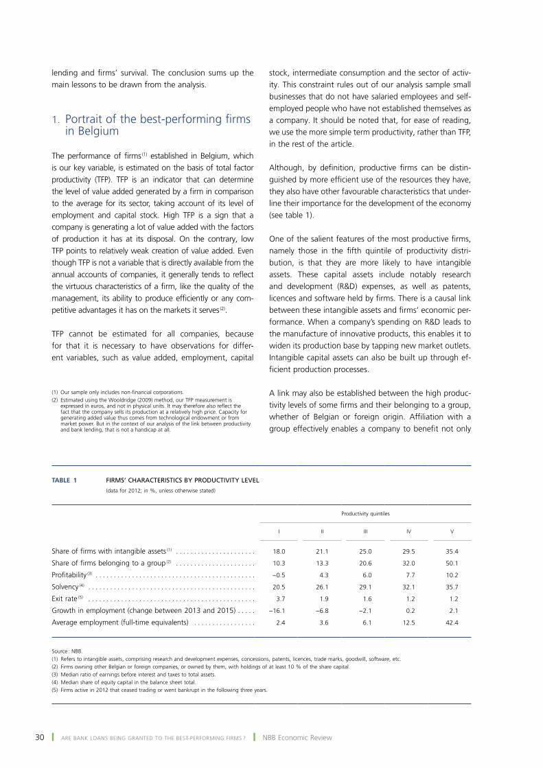
30 ❙ ARE BANk loANS BEINg gRANtED to tHE BESt‑pERfoRmINg fIRmS ? ❙ NBB Economic Review
lending and firms’ survival. The conclusion sums up the main lessons to be drawn from the analysis.
1. Portrait of the best-performing firms in Belgium
The performance of firms (1) established in Belgium, which is our key variable, is estimated on the basis of total factor productivity (TFP). TFP is an indicator that can determine the level of value added generated by a firm in comparison to the average for its sector, taking account of its level of employment and capital stock. High tfp is a sign that a company is generating a lot of value added with the factors of production it has at its disposal. On the contrary, low TFP points to relatively weak creation of value added. Even though tfp is not a variable that is directly available from the annual accounts of companies, it generally tends to reflect the virtuous characteristics of a firm, like the quality of the management, its ability to produce efficiently or any com‑petitive advantages it has on the markets it serves (2).
tfp cannot be estimated for all companies, because for that it is necessary to have observations for differ‑ent variables, such as value added, employment, capital
stock, intermediate consumption and the sector of activ‑ity. this constraint rules out of our analysis sample small businesses that do not have salaried employees and self‑employed people who have not established themselves as a company. It should be noted that, for ease of reading, we use the more simple term productivity, rather than TFP, in the rest of the article.
Although, by definition, productive firms can be distin‑guished by more efficient use of the resources they have, they also have other favourable characteristics that under‑line their importance for the development of the economy (see table 1).
One of the salient features of the most productive firms, namely those in the fifth quintile of productivity distri‑bution, is that they are more likely to have intangible assets. these capital assets include notably research and development (R&D) expenses, as well as patents, licences and software held by firms. There is a causal link between these intangible assets and firms’ economic per‑formance. When a company’s spending on R&D leads to the manufacture of innovative products, this enables it to widen its production base by tapping new market outlets. Intangible capital assets can also be built up through ef‑ficient production processes.
A link may also be established between the high produc‑tivity levels of some firms and their belonging to a group, whether of Belgian or foreign origin. Affiliation with a group effectively enables a company to benefit not only
(1) Our sample only includes non-financial corporations.(2) Estimated using the Wooldridge (2009) method, our TFP measurement is
expressed in euros, and not in physical units. It may therefore also reflect the fact that the company sells its production at a relatively high price. capacity for generating added value thus comes from technological endowment or from market power. But in the context of our analysis of the link between productivity and bank lending, that is not a handicap at all.
Table 1 FIRMS’ CHARACTERISTICS BY PRODUCTIVITY LEVEL
(data for 2012; in %, unless otherwise stated)
Productivity quintiles
I
II
III
IV
V
Share of firms with intangible assets (1) . . . . . . . . . . . . . . . . . . . . . . 18.0 21.1 25.0 29.5 35.4
Share of firms belonging to a group (2) . . . . . . . . . . . . . . . . . . . . . . 10.3 13.3 20.6 32.0 50.1
Profitability (3) . . . . . . . . . . . . . . . . . . . . . . . . . . . . . . . . . . . . . . . . . . . . −0.5 4.3 6.0 7.7 10.2
Solvency (4) . . . . . . . . . . . . . . . . . . . . . . . . . . . . . . . . . . . . . . . . . . . . . . 20.5 26.1 29.1 32.1 35.7
Exit rate (5) . . . . . . . . . . . . . . . . . . . . . . . . . . . . . . . . . . . . . . . . . . . . . . 3.7 1.9 1.6 1.2 1.2
Growth in employment (change between 2013 and 2015) . . . . . −16.1 −6.8 −2.1 0.2 2.1
Average employment (full-time equivalents) . . . . . . . . . . . . . . . . . 2.4 3.6 6.1 12.5 42.4
Source : NBB.(1) Refers to intangible assets, comprising research and development expenses, concessions, patents, licences, trade marks, goodwill, software, etc.(2) Firms owning other Belgian or foreign companies, or owned by them, with holdings of at least 10 % of the share capital.(3) Median ratio of earnings before interest and taxes to total assets.(4) Median share of equity capital in the balance sheet total.(5) Firms active in 2012 that ceased trading or went bankrupt in the following three years.

31December 2017 ❙ ARE BANk loANS BEINg gRANtED to tHE BESt‑pERfoRmINg fIRmS ? ❙
from shared intangible assets but also from productivity gains stemming from economies of scale.
The profitability of firms is also closely correlated to their productivity levels. The most productive firms post a prof‑itability ratio with a median value of more than 10 %, while the companies in the first productivity quintile, that is, the less efficient ones, frequently suffer losses. However, it should be noted that there is no one-to-one connection between productivity and profitability, and for different reasons too. for instance, at a given perfor‑mance level, a company whose return on production is distributed more widely among workers than equity hold‑ers registers a lower profitability rate. Apart from profit‑ability, the better financial health of the most productive firms is also reflected in higher solvency ratios, thanks to retained earnings and accumulated reserves.
Lastly, the fact that they manage to generate profits naturally enables the more productive businesses to guarantee their future and to grow. That is largely reflected in lower rates of bankruptcy or cessation of activities, as well as much stronger employment growth than that for low-performing firms (1). these differences in terms of exit rates and employment trends are in a way a reflection of a process of creative destruction and efficient reallocation of factors of production, where less productive and less profitable firms go out of business, while the higher performers expand. Hence, the weight of successful firms in the total economy, whether meas‑ured on the basis of employment, capital stock or value added, is relatively high.
2. Allocation of bank loans to companies
2.1 Overview
Generally speaking, the most productive firms take up the lion’s share of all loans granted by resident banks. As chart 1 shows, 55 % of outstanding loans are concentrated in the hands of companies in the fifth productivity quintile, compared with barely 20, 12, 8 and 4 % respectively for the lower quintiles. However, this observation can be qualified. In fact, the best-per‑forming firms account for 59 % of employment, hold 62 % of the capital stock and generate 69 % of value
added. Productive firms have admittedly contracted more loans, but not proportionately to their weight in the economy.
2.2 factors affecting the allocation of credit
Alternative sources of finance
The reason why bank loans to productive firms are not in proportion to their weight in the economy is partly because these companies are more often likely to have access to alternative means of finance, such as bond is‑sues for example. Moreover, the best-performing firms belong to a group more often than not (see above). So, they can count on privileged sources of funding, like equity stakes or inter-company loans. So, it is hardly surprising that they generally tend to be better capitalised during their first few years of existence and benefit more often from non-bank loans (see chart 2). Of course, the least productive firms fund their busi‑ness even more from their own capital. However, that is more a question of need, because their low profitability and the resultant scale of losses carried over limit their access to bank loans.
(1) It is worth noting that the period 2013-2015, for which growth in employment has been calculated in table 1, was rather unfavourable in terms of labour market developments. The year 2013, in particular, was marked by heavy job losses. As can be seen from the data presented in table 1, it was above all the firms with the weakest performance that were affected by these job losses.
Chart 1 BREAKDOWN OF BANK LOANS PER PRODUCTIVITY QUINTILE
(data for 2015, in % of the total)
0
10
20
30
40
50
60
70
80
I II III IV V
Loans (1)
Employment (2)
Capital stock (3)
Value added
Productivity quintiles
Source : NBB.(1) outstanding total of long‑term loans authorised.(2) Expressed as full-time equivalents.(3) Non-financial fixed assets.

32 ❙ ARE BANk loANS BEINg gRANtED to tHE BESt‑pERfoRmINg fIRmS ? ❙ NBB Economic Review
It is also quite likely that the higher capitalisation of young and very productive enterprises partly reflects the fact that they turn more frequently to funding from venture capital,
which may come from business angels, specialised financ‑ing companies or crowdfunding platforms, for instance. However, the data at our disposal do not enable any systematic identification of firms that have benefited from these sources of finance.
Productivity
As mentioned before, the most productive firms gen‑erally tend to be more profitable and bigger than the others, just as they have easier access to other sources of finance. This combination of characteristics specific to successful companies makes it hard to assess the precise role played by productivity in the allocation of bank loans. A descriptive approach, like that followed in section 2.1, can actually lead to this factor being wrongly attributed to an effect that in fact results from other features of these firms, like their size or profitability.
to make up for this inherent shortcoming of the descrip‑tive analysis, we resort to a multivariate approach, de‑scribed in the box below. This method has the advantage of accurately pinpointing the link between new loans (1) and each factor considered in isolation. Moreover, we focus on the determinants of obtaining a loan rather than on the amount borrowed. This is mostly influenced by the scale of the funding requirements. Under our analysis, we are nevertheless not trying to establish whether firms are
Chart 2 RECOURSE TO ALTERNATIVE MEANS OF FINANCE BY YOUNG FIRMS (1)
(percentage of long-term funding requirements (2), data for 2015)
I II III IV V–40
–20
0
20
40
60
80
100
F
Productivity quintiles
Reserves and accumulated profits (losses)
Non-bank long-term loans (3)
Total
Capital
Source : NBB.(1) Firms that have been active for at least five years. (2) Long-term funding requirements are approximated by the sum of fixed assets
and working capital requirements.(2) Includes both bond issues and other non‑bank loans, such as intra‑group
financing and loans extended by private individuals.
(1) New loans refer to new lender-borrower relationships between a bank and a company and additional loans.
Box – methodology
In order to determine the characteristics of firms that manage to get loans from banks, we have put data from the Central Balance Sheet Office (CBSO) together with information from the Central Corporate Credit Register (CCCR). The CBSO provides information on the features of each firm, such as employment, capital stock, value added, sec‑tor of activity, etc. Its data also enables an estimate of TFP. Data from the CCCR give the amount borrowed, per bank and per borrowing enterprise. The term ‘loans’ refers to the type of loan that banks typically grant companies to meet their long-term funding requirements, that is, mainly fixed-term loans and instalment loans (1). our sample of data covers the period 2005-2015.
The econometric approach selected is based on a probit-type regression analysis, which measures the impact of each factor on a binary variable that equals 1 in the case of a new bank loan and 0 in the other cases. Among the explanatory factors, we have included productivity, profitability, solvency (2), liquidity requirements (3), size, age,
4
(1) This definition excludes short-term credit facilities. They are nevertheless taken into account in the third part of this article.(2) Share of equity capital in the balance sheet total.(3) Liquidity requirements are estimated on the basis of the difference between the working capital requirement and actual working capital. A firm is deemed to
be facing liquidity needs once this difference is positive.

33December 2017 ❙ ARE BANk loANS BEINg gRANtED to tHE BESt‑pERfoRmINg fIRmS ? ❙
getting appropriate funding, but rather to profile those firms that get a loan and of those that are turned down.
To begin with, we take a look at the results obtained for productivity. the predicted probability (1) of a new loan works out at 19 % for firms in the first productivity quin‑tile and respectively 21, 22, 22 and 20 % for those in the subsequent quintiles (see upper left-hand panel of chart 3). Expressed as a percentage change when the predicted probability for the first quintile is taken as a benchmark, the probabilities of a new loan for the following quintiles are respectively 11, 16, 15 and 5 % higher than it.
This result leads us to pinpoint two elements. On the one hand, the banks take companies’ economic performance into consideration when it comes to granting them loans. Low-performing firms are actually having difficulty in get‑ting a loan from a bank. However, the allocation of loans is relatively insensitive to productivity. the predicted probabil‑ity of getting a new bank loan is virtually identical for the second, third and fourth productivity quintiles. On the oth‑er hand, the fact that probability is lower for the last quin‑tile indicates that access to new credit is relatively limited for the most productive companies. Even if we control for a certain number of demand factors, such as membership of a group or its legal form (and thus its possible recourse to equity finance, as is the case with limited companies for example), the list cannot be exhaustive. So, we cannot
measure the ease with which a company can turn to other forms of alternative funding, like venture capital. the result for high-performing firms is therefore difficult to interpret. On the whole, these estimates are still enough to point up the highly ambiguous connection between new loans and firms’ productivity levels.
the exercise carried out so far on a global level can also be broken down individually for each of the big four commercial banks active in Belgium (2). We can then see that the relationship between new loans and firms’ productivity varies significantly from one large bank to another. For banks 1 and 2, the connection between new loans granted and companies’ productivity is a lot more pronounced. for instance, in the case of bank 2, firms in the fourth and fifth productivity quintiles have respectively 37 and 25 % more chance of being given a new loan than those in the first quintile. By contrast, banks 3 and 4 are a lot less sensitive to productivity. in the case of bank 4, the predicted probability of enter‑prises in the fourth quintile rose by only 9 %, while the more productive companies have less chance of getting a new loan than low-performing firms.
sector of activity, legal form, whether the company invests or not, whether it belongs to a group or not (1), as well as cyclical effects or those induced by developments in the macrofinancial environment, which are captured by annual binary variables. In order to counter endogeneity risks, our probit model relates any new loans obtained during a given accounting year to characteristics of firms as observed when closing the previous year’s annual accounts (2). The results of this regression are given in table A.1 of the annex.
for each variable, like productivity for example, the probit model makes it possible to estimate a predicted prob‑ability. This provides an average response, calculated for the whole sample, for different given values for the vari‑able considered, while keeping the other variables unchanged. The predicted probability has the big advantage of not being skewed by any possible correlations between the various explanatory variables. As the sample contains almost 100 000 observations, our estimates for each factor considered separately are robust.
Apart from the binary approach, we have also carried out an analysis focusing on the amounts of loans authorised, the results of which are also given in table A.1. It shows that the variables determining whether a firm has a loan or not also affect the authorised amounts. Overall, the results of this exercise are very similar to the findings of the binary approach. This is why this article only discusses the findings using this approach.
(1) The group may be purely domestic, international with a Belgian parent company or international with a foreign parent company.(2) The objective here is to determine the influence of each factor on bank loans, and not the other way round. Yet, bank loans themselves directly affect certain factors,
like solvency for instance. In fact, they automatically reduce the share of equity capital in the balance sheet total. In order to limit the influence of bank loans on solvency, bank loans granted during the year t are considered in relation to solvency in t‑1.
(1) The average predicted probability gives the average response for the whole sample if the productivity of all the firms takes a given value (successively the average level of the first quintile, the second quintile, etc.), while keeping all the other firm characteristics unchanged. The predicted probability has the big advantage of not being skewed by any correlations between the characteristics.
(2) For confidentiality reasons, the big four banks are not identified and have randomly been attributed a number between 1 and 4.

34 ❙ ARE BANk loANS BEINg gRANtED to tHE BESt‑pERfoRmINg fIRmS ? ❙ NBB Economic Review
Solvency and profitability
A similar exercise to that carried out for productivity can be performed for solvency and for profitability, two elements that the banks generally tend to take into account when they are assessing default risks, notably by reference to their internal models.
The relationship between firms’ solvency, that is, the share of equity – which includes reserves and reinvested earnings – in their balance sheet total, and the predicted probability of a new loan is non-linear. As the centre panel of chart 3 shows, it takes the shape of an upside down "U". The probability is lower for both the least solvent and the most solvent companies. The first find‑ing is of course to do with credit institutions’ lack of confidence in enterprises with excessive debt levels in relation to their equity capital and / or an accumulation of losses carried over. the second most probably comes from a demand effect. The more highly capitalised firms or those that have built up substantial reserves that have been added to over the years are in fact the most likely to fund themselves, by using their available cash as a substitute for bank credit.
The result for profitability – which we measure by the ratio of earnings before interest and taxes to total assets – is clear. The most profitable enterprises post much higher probabilities of getting a new loan. The interpretation of this relationship is fairly intuitive : sufficiently high operat‑ing results send a very strong signal to banks because they are a kind of guarantee of a firm’s ability to service its debt.
The sensitivity of new lending to solvency or productivity varies from one large bank to another, although to a much lesser extent than for productivity (see below-centre and right panels of chart 3). The sensitivity of banks 3 and 4 is identical to that applying on average to all banks. It is inter‑esting to note that the relationship between new loans and profitability is strongest for bank 1, which is already highly sensitive to productivity.
generally speaking, the importance that credit institutions attach to accounting ratios for the financial health of bor‑rowers is largely based on the assumption that they serve as good predictors of the sustainability of firms and their future ability to honour their financial obligations. In fact, 16 % of firms from the first profitability quintile in 2010 had ceased
Chart 3 LINKS BETWEEN PRODUCTIVITY, SOLVENCY, PROFITABILITY AND NEW LOANS
(estimates for the period 2006-2015)
0
10
20
30
40
0
10
20
30
40
0
10
20
30
40
–10
0
10
20
30
40
50
–10
0
10
20
30
40
50
–10
0
10
20
30
40
50
I II III IV V I II III IV V I II III IV V
I II III IV V I II III IV V I II III IV V
PRODUCTIVITY (QUINTILES) SOLVENCY (QUINTILES) PROFITABILITY (QUINTILES)
Percentages
Percentage change compared with quintile I
Bank 1 Bank 2 Bank 3 Bank 4
Predicted probability of a new loan :
Source : NBB.

35December 2017 ❙ ARE BANk loANS BEINg gRANtED to tHE BESt‑pERfoRmINg fIRmS ? ❙
trading or been declared bankrupt five years later (1), while this proportion dropped to just 5 % for the most profitable companies (see chart 4).
While unfavourable ratios really do reflect a risk of default at a given moment in time, this risk can nev‑ertheless evolve over time, and the risk assessment may therefore be surrounded by uncertainty. Earnings generated by a firm over one accounting year are not necessarily representative of its future profits. The observable trend here is that just 21 % of enterprises belonging to the first profitability quintile in 2010 were still there in 2015, while 14 % moved into the fifth quintile.
By way of comparison, the other indicators studied, no‑tably productivity, do not show any such instability over time (see chart 5). These findings suggest that a discrimi‑nating indicator for bank lending, in this case profitability, is relatively unstable over time.
Age of the firms
A firm’s age may have significant influence on the probability of having loans from the bank. Among the population of firms that had a bank loan in 2015, there is a higher proportion of older businesses (see left‑hand panel of chart 6). So, young enterprises seem to encounter some difficulty in getting a bank loan. This fact is backed up by the obvious difficulty in getting a loan for the first time (see right-hand panel of chart 6). Compared with firms that have not yet taken out any loans, those which have already had at least one are twice as likely to be able to contract a new loan or obtain an additonal loan.
Investment
Bank loans are naturally used for meeting financing re‑quirements. They are more often granted to enterprises that invest. The predicted probability of getting a new loan is only 12 % when the firm does not invest, but is much higher when the firm does invest (see chart 7). A big difference depending on the type of investment is nevertheless observed.
the predicted probability goes up sharply in the case of investment in tangible assets : rising to 37 %, even to as much as 45 % for investment in tangible and intangible assets at the same time. on the other hand, investing
(1) This exit rate does not take account of company exits following mergers or acquisitions.
Chart 4 MOVEMENTS OF FIRMS ACROSS THE PROFITABILITY DISTRIBUTION (1)
(percentages)
I II III IV V0
10
20
30
40
50
60
70
80
90
100
Quintile in 2010
Exit
Quintile I
Quintile II
Quintile III
Quintile IV
Quintile V
Status in 2015
Source : NBB.(1) measured on the basis of the ratio of earnings before interest and taxes to total
assets.
Chart 5 MOVEMENTS OF FIRMS ACROSS THE PRODUCTIVITY DISTRIBUTION
(percentages)
I II III IV V0
10
20
30
40
50
60
70
80
90
100
Quintile in 2010
Exit
Quintile I
Quintile II
Quintile III
Quintile IV
Quintile V
Status in 2015
Source : NBB.

36 ❙ ARE BANk loANS BEINg gRANtED to tHE BESt‑pERfoRmINg fIRmS ? ❙ NBB Economic Review
solely in intangible assets has a lot less influence on the probability of getting a new loan, because it only scores 17 %. This finding is probably to do with the fact that, unlike investment in tangible assets, intangible assets can rarely be used as collateral with the banks.
3. Bank loans and firms’ survival
The link between business credit and investment takes us back to the essential role that the banking system plays in economic development. By granting loans to firms, banks are notably giving them the possibility of putting in place the production capacity needed to implement their pro‑jects. Apart from funding investment projects, bank loans can also cover working capital requirements. Businesses must have sufficient cash reserves to ensure their day-to-day operations, especially for paying wages or suppliers’ invoices. Without these liquid assets, firms run the risk of defaulting.
Bank credit can therefore contribute to the viability and sustainability of business enterprises. As chart 8 illus‑trates, firms that have already obtained a loan run less risk of going out of business than those that have not benefited from this source of funding, regardless of their productivity level. this emphasises the fact that, even in the case of the best‑performing companies, having a bank loan – and, more generally, long‑term sources of funding – proves to be a crucial factor of survival.
Of course, the causal link between getting credit and a firm’s probability of survival is not one-sided. Productive enterprises may see their loan applications turned down because they present characteristics with signs of im‑minent failure, such as low profitability. However, the favourable effect that bank lending exerts on the sus‑tainability of firms is statistically significant, even when
Chart 6 DIFFICULTY IN OBTAINING A FIRST BANK LOAN
3-4
5-6
7-9
10-1
4
15-1
91 2
40
45
50
55
60
65
70
0
5
10
15
20
25
30
20 a
nd +
PREDICTED PROBABILITY OF HAVING A LOAN(in %, 2015)
Age classes (1)
Firms with no loan Firms with a loan
PREDICTED PROBABILITY OF A NEW LOAN(in %, 2006-2015)
Source : NBB.(1) Number of years since the firm was established.
Chart 7 LOANS USED MOSTLY TO FINANCE INVESTMENT IN TANGIBLE CAPITAL, LESS SO IN INTANGIBLE ASSETS
(predicted probability of a new loan in %, estimates for the period 2006-2015)
0
10
20
30
40
50
No
inve
stm
ent
Inve
stm
ent
in
inta
ngib
le a
sset
s
Inve
stm
ent
in
tang
ible
ass
ets
Inve
stm
ent
in b
oth
tang
ible
an
d in
tang
ible
ass
ets
Source : NBB.

37December 2017 ❙ ARE BANk loANS BEINg gRANtED to tHE BESt‑pERfoRmINg fIRmS ? ❙
isolated from the influence of other factors likely to affect their survival.
our estimates (1), presented in table A.2 in the Annex, effectively confirm that, ceteris paribus, bank loans are systematically associated with a greater probability of survival. this effect is all the more important for the more productive enterprises, which suggests that, on average, bank loans have a more direct bearing on these firms’ chances of survival than is the case for less productive firms. By contrast, short-term credit facilities are not associated with higher chances of survival. They even have a significant influence on the exit probability of low-performers, reflecting the risk of bankruptcy related to an excessively heavy degree of short‑term indebtedness that they carry (2).
conclusion
Bank loans are often a crucial ingredient for the success of projects carried out by businesses. they enable companies, notably the best-performing ones, to have a sufficiently solid financial base to ensure their development. And in lending funds, the banks themselves make a significant contribution to economic growth and job creation.
The findings presented in this article nevertheless suggest that the most productive firms are taking up a smaller
proportion of bank loans than expected given their weight in the economy. that is partly because the best‑perform‑ing companies benefit more extensively from alternative sources of funding, such as intra-group financing, and therefore do not resort systematically to bank loans to finance their projects. Nevertheless, our analysis points to certain factors that might hinder bank‑managed funds from being channelled towards the best-performing firms. More specifically, a high risk profile makes it harder to get access to bank loans, even if the firm’s production model or its positioning on the market are enabling it to perform well, or at least give it the potential to become a success‑ful business.
In this respect, the various determinants of bank lend‑ing highlighted in this article make it possible to profile the firm that is doing well, but still likely to encounter difficulties in getting a loan. This is typically a newly established firm and which does not belong to a group. It is still not in a position to put forward any convincing guarantees of its project’s viability on the basis of its first accounting results, even though these results may improve considerably in the next few years. Nor does it have any credit history proving its ability to repay its debts. Besides, when its project is largely based on the use of intangible assets, such as a patent for example, it can offer the banks very little in the way of tangible guarantees when applying for a loan.
This attitude towards risk being taken by banks is justi‑fied from the financial stability point of view. It is even encouraged by prudential regulations subjecting banks to capital requirements proportional to the risky nature of the components on the assets side of their balance sheets, including corporate loans. that being said, the mere fact that some young firms with great potential can see their access to bank lending restricted owing to the uncertainty surrounding their viability stresses the importance of alternative sources of funding, and in particular venture capital finance.
By strengthening the equity capital invested by entre‑preneurs, funding through venture capital gives firms just starting out a chance to have a large enough capital
(1) These estimates are based on a discrete choice model, which includes among the explanatory variables taken into consideration the amounts granted as bank loans, whose perimeter is determined in the same way as in the previous part, that is, by incorporating the types of loans normally used for long‑term funding. Also included in the specification, via an additional variable, are loans obtained through short‑term instruments, such as authorised overdrafts on bank accounts. The respective effects of these two categories of loans on a firm’s exit probability have been estimated on the basis of a complementary log-log (cloglog) type model (see Tsoukas, 2011), after controling for the effects of several control variables.
(2) This is also the reason why these short-term credit instruments have not been incorporated into the analysis presented in the second part.
Chart 8 EXIT RATE FOR COMPANIES ACCORDING TO THEIR PRODUCTIVITY LEVEL
(percentages of firms active in 2012 that had ceased trading or gone into bankruptcy within the next three years))
I II III IV V0
1
2
3
4
5
6
Firms with no loans
Firms with loans
Productivity quintiles
Source : NBB.

38 ❙ ARE BANk loANS BEINg gRANtED to tHE BESt‑pERfoRmINg fIRmS ? ❙ NBB Economic Review
buffer to absorb any losses incurred during their start‑up phase. Some initiatives have recently been taken in Belgium, including at regional level, to promote or sup‑port this funding method (1). through its capital markets union project, the European commission is also plan‑ning to take a number of measures to this end. If they re‑ally do help channel funds into entrepreneurial ventures
that generate the most value added, these initiatives will certainly be relevant.
(1) this mainly involves the ‘tax shelter’, a tax incentive offered to private individuals who invest in young enterprises, and the establishment of a regulatory framework tailor-made for crowdfunding platforms, which aims in particular to verify the professional skills of crowdfund managers and to protect investors. This regulatory approval framework was laid down by the Law of 18 December 2016. public funding initiatives have also been taken at regional level. Among these are most notably Seed & Early Stage in flanders, investment aid in Brussels and action taken by SoWAlfIN and SRIW in Wallonia.

39December 2017 ❙ ARE BANk loANS BEINg gRANtED to tHE BESt‑pERfoRmINg fIRmS ? ❙
Annexes
Table a.1 PROBABILITY OF A NEW LOAN AND AMOUNTS AUTHORISED
(data for the period 2006-2015)
Explanatory variables
Binary approach (loan=1, no loan=0)
Amounts authorised
(Marginal effect)
(Predicted probability)
(Average marginal effect (1))
Productivity (TFP) in t −1Quintile I . . . . . . . . . . . . . . . . . . . . . . . . . . . . . . . . . . . . . . . . . . . . . 18.9*** – –Quintile II . . . . . . . . . . . . . . . . . . . . . . . . . . . . . . . . . . . . . . . . . . . . . 21.0*** 11.2*** 1.1***Quintile III . . . . . . . . . . . . . . . . . . . . . . . . . . . . . . . . . . . . . . . . . . . . 21.9*** 15.5*** 1.5***Quintile IV . . . . . . . . . . . . . . . . . . . . . . . . . . . . . . . . . . . . . . . . . . . . 21.8*** 15.3*** 1.4***Quintile V . . . . . . . . . . . . . . . . . . . . . . . . . . . . . . . . . . . . . . . . . . . . 19.9*** 5.0 0.5
Profitability in t −1Quintile I . . . . . . . . . . . . . . . . . . . . . . . . . . . . . . . . . . . . . . . . . . . . . 17.0*** – –Quintile II . . . . . . . . . . . . . . . . . . . . . . . . . . . . . . . . . . . . . . . . . . . . . 20.2*** 19.1*** 1.8***Quintile III . . . . . . . . . . . . . . . . . . . . . . . . . . . . . . . . . . . . . . . . . . . . 21.5*** 26.5*** 2.4***Quintile IV . . . . . . . . . . . . . . . . . . . . . . . . . . . . . . . . . . . . . . . . . . . . 21.9*** 28.8*** 2.6***Quintile V . . . . . . . . . . . . . . . . . . . . . . . . . . . . . . . . . . . . . . . . . . . . 22.2*** 30.5*** 2.7***
Solvency in t −1Quintile I . . . . . . . . . . . . . . . . . . . . . . . . . . . . . . . . . . . . . . . . . . . . . 17.8*** – –Quintile II . . . . . . . . . . . . . . . . . . . . . . . . . . . . . . . . . . . . . . . . . . . . . 22.4*** 25.8*** 2.3***Quintile III . . . . . . . . . . . . . . . . . . . . . . . . . . . . . . . . . . . . . . . . . . . . 22.8*** 27.6*** 2.4***Quintile IV . . . . . . . . . . . . . . . . . . . . . . . . . . . . . . . . . . . . . . . . . . . . 21.8*** 22.0*** 1.9***Quintile V . . . . . . . . . . . . . . . . . . . . . . . . . . . . . . . . . . . . . . . . . . . . 18.0*** 0.9 −0.1
Investment (2)
None . . . . . . . . . . . . . . . . . . . . . . . . . . . . . . . . . . . . . . . . . . . . . . . . 11.9*** – –In tangible assets . . . . . . . . . . . . . . . . . . . . . . . . . . . . . . . . . . . . . . 37.0*** 209.6*** 1.2***In intangible assets . . . . . . . . . . . . . . . . . . . . . . . . . . . . . . . . . . . . . 16.6*** 39.0*** 0.3***In both tangible and intangible assets . . . . . . . . . . . . . . . . . . . . 45.0*** 276.6*** –
Size category (number of employees)0 . . . . . . . . . . . . . . . . . . . . . . . . . . . . . . . . . . . . . . . . . . . . . . . . . . . . 18.4*** – –1-9 . . . . . . . . . . . . . . . . . . . . . . . . . . . . . . . . . . . . . . . . . . . . . . . . . . 20.4*** 10.9*** 1.1***10-49 . . . . . . . . . . . . . . . . . . . . . . . . . . . . . . . . . . . . . . . . . . . . . . . . 23.1*** 25.8*** 2.2***50-249 . . . . . . . . . . . . . . . . . . . . . . . . . . . . . . . . . . . . . . . . . . . . . . . 19.0*** 3.6 −0.4250 or more . . . . . . . . . . . . . . . . . . . . . . . . . . . . . . . . . . . . . . . . . . 13.6*** −25.9*** −4.9***
Age category (number of years)1 year . . . . . . . . . . . . . . . . . . . . . . . . . . . . . . . . . . . . . . . . . . . . . . . . 25.8*** – –2 years . . . . . . . . . . . . . . . . . . . . . . . . . . . . . . . . . . . . . . . . . . . . . . . 22.8*** −11.6*** −1.4***3-4 years . . . . . . . . . . . . . . . . . . . . . . . . . . . . . . . . . . . . . . . . . . . . . 22.0*** −14.8*** −1.9***5-6 years . . . . . . . . . . . . . . . . . . . . . . . . . . . . . . . . . . . . . . . . . . . . . 21.1*** −18.0*** −2.4***7-9 years . . . . . . . . . . . . . . . . . . . . . . . . . . . . . . . . . . . . . . . . . . . . . 21.1*** −18.1*** −2.4***10-14 years . . . . . . . . . . . . . . . . . . . . . . . . . . . . . . . . . . . . . . . . . . . 21.0*** −18.4*** −2.4***15-19 years . . . . . . . . . . . . . . . . . . . . . . . . . . . . . . . . . . . . . . . . . . . 20.9*** −18.9*** −2.4***20 years or more . . . . . . . . . . . . . . . . . . . . . . . . . . . . . . . . . . . . . . 20.1*** −22.1*** −2.9***
Already has a loan?No . . . . . . . . . . . . . . . . . . . . . . . . . . . . . . . . . . . . . . . . . . . . . . . . . . 12.9*** – –Yes . . . . . . . . . . . . . . . . . . . . . . . . . . . . . . . . . . . . . . . . . . . . . . . . . . 24.0*** 86.2*** 5.9***
Liquidity requirement in t −1 (3)
No . . . . . . . . . . . . . . . . . . . . . . . . . . . . . . . . . . . . . . . . . . . . . . . . . . 19.2*** – –Yes . . . . . . . . . . . . . . . . . . . . . . . . . . . . . . . . . . . . . . . . . . . . . . . . . . 23.1*** 20.4*** 2.0***
Part of a groupNo . . . . . . . . . . . . . . . . . . . . . . . . . . . . . . . . . . . . . . . . . . . . . . . . . . 21.2*** – –Yes . . . . . . . . . . . . . . . . . . . . . . . . . . . . . . . . . . . . . . . . . . . . . . . . . . 19.5*** −8.0*** −0.8***
Fixed effects : industry (2-digit NACE) . . . . . . . . . . . . . . . . . . . . Yes Yes Yes
Fixed effects : legal form . . . . . . . . . . . . . . . . . . . . . . . . . . . . . . . . Yes Yes Yes
Fixed effects : years . . . . . . . . . . . . . . . . . . . . . . . . . . . . . . . . . . . . . Yes Yes Yes
Number of observations . . . . . . . . . . . . . . . . . . . . . . . . . . . . . . . . . . 942 496 942 496 942 496
Source: NBB.(1) The average marginal effect corresponds to the (percentage) change in the probability of a new loan in comparison with the reference group.(2) For the binary approach (see the first two columns), investment is a binary variable that takes a value of 1 if there is any investment and 0 if otherwise. For the authorised
amount approach (see the last column), investment is a sum expressed in logs.(3) Liquidity requirements estimated on the basis of the difference between the working capital requirement and actual working capital. A firm is deemed to be facing liquidity
needs once this difference is positive.* significant at 10 % ; ** significant at 5 % ; *** significant at 1 %.

40 ❙ ARE BANk loANS BEINg gRANtED to tHE BESt‑pERfoRmINg fIRmS ? ❙ NBB Economic Review
Table a.2 DETERMINANTS OF A FIRM’S PROBABILITY OF EXIT
(marginal effects (1) estimated using a complementary log-log model, data for the period 2006-2015)
Explanatory variables
Productivity quintiles
I
II
III
IV
V
Credit used (in % of balance sheet total) . . . . . . . . . . . . . . . . . . . . −0.58*** −1.26*** −2.40*** −2.42*** −3.61***
Credit lines used (in % of balance sheet total) . . . . . . . . . . . . . . . 0.26** −0.40 −0.22 −1.00* −0.19
Employment in full-time equivalents (logarithm) . . . . . . . . . . . . . . −0.08*** −0.18*** −0.17*** −0.24*** −0.21***
Non-financial fixed assets (logarithm) . . . . . . . . . . . . . . . . . . . . . . . −0.16*** −0.23*** −0.27*** −0.27*** −0.25***
Earnings before interest and taxes (in % of balance sheet total) . . . . . . . . . . . . . . . . . . . . . . . . . . . . . . −0.92*** −1.14*** −0.47*** −0.36** −0.07
Part of a group . . . . . . . . . . . . . . . . . . . . . . . . . . . . . . . . . . . . . . . . . . −0.04 −0.33*** −0.32*** −0.36*** −0.50***
Age category (base: 10-14 years)
Less than a year . . . . . . . . . . . . . . . . . . . . . . . . . . . . . . . . . . . . . . . −0.32 −0.27 0.04 −0.53 −0.13
1 year . . . . . . . . . . . . . . . . . . . . . . . . . . . . . . . . . . . . . . . . . . . . . . . . 0.22** −0.21 −0.27 −0.75** −0.13
2 years . . . . . . . . . . . . . . . . . . . . . . . . . . . . . . . . . . . . . . . . . . . . . . . 0.15** 0.60 −0.05 −0.31*** −0.26
3-4 years . . . . . . . . . . . . . . . . . . . . . . . . . . . . . . . . . . . . . . . . . . . . . 0.16*** 0.08 −0.19 −0.34*** −0.25
5-6 years . . . . . . . . . . . . . . . . . . . . . . . . . . . . . . . . . . . . . . . . . . . . . 0.14** −0.34 −0.10 −0.54*** −0.05
7-9 years . . . . . . . . . . . . . . . . . . . . . . . . . . . . . . . . . . . . . . . . . . . . . 0.18*** −0.25 0.00 −0.28*** −0.14
15-19 years . . . . . . . . . . . . . . . . . . . . . . . . . . . . . . . . . . . . . . . . . . . 0.17*** 0.17** 0.26*** −0.06 −0.06
20 years or more . . . . . . . . . . . . . . . . . . . . . . . . . . . . . . . . . . . . . . 0.43*** 0.37*** 0.32*** 0.02 −0.13
Fixed effects : years . . . . . . . . . . . . . . . . . . . . . . . . . . . . . . . . . . . Yes Yes Yes Yes Yes
Number of observations . . . . . . . . . . . . . . . . . . . . . . . . . . . . . . . . 184 024 185 732 185 878 185 515 183 076
Source : NBB.(1) A marginal effect corresponds to the impact of the change in one unit of an explanatory variable on the logarithm of the exit probability.* significant at 10 %; ** significant at 5 %; *** significant at 1 %.

41December 2017 ❙ ARE BANk loANS BEINg gRANtED to tHE BESt‑pERfoRmINg fIRmS ? ❙
Bibliography
Adler G., R. Duval, D. Furceri, S. K. Çelik, K. Koloskova and M. Poplawski-Ribeiro (2017), Gone with the Headwinds : Global Productivity, Imf Staff discussion note 17 / 04.
Besley T., I. Roland and J. Van Reenen (2017), Credit Market Frictions and the Productivity Slowdown, mimeo.
Duval R., G.H. Hong and Y. Timmer (2017), Financial frictions and the great productivity slowdown, Imf Working paper 17 / 129.
McGowan M. A., D. Andrews and V. Millot (2017), The walking dead ? Zombie firms and productivity performance in OECD countries, OECD Working Paper 2017 / 4.
Tsoukas S. (2011), “Firm survival and financial development : Evidence from a panel of emerging Asian economies”, Journal of Banking & Finance, 35, 1736-1752.
Wooldridge J. (2009), “On estimating firm-level production functions using proxy variables to control for unobservables”, Economics Letters, 104(3), 112-114.

43December 2017 ❙ tHE NEgAtIvE INtERESt RAtE polIcY IN tHE EuRo AREA AND tHE SupplY of BANk loANS ❙
the negative interest rate policy in the euro area and the supply of bank loans
M. de Sola PereaM. Kasongo Kashama
Introduction
From the summer of 2014 onwards, the Governing Council of the European Central Bank (ECB) took a series of measures aimed at further easing its monetary policy stance in the face of falling inflation. These measures include the gradual lowering of the deposit facility interest rate – the benchmark rate for euro area markets in times of ample liquidity – taking it into negative territory. This key policy interest rate, which had stood at 0 % since July 2012, was cut to –0.1 % in June 2014, then to –0.2 % in September 2014, and to –0.3 % in December 2015, fi‑nally reaching a low of –0.4 % in March 2016.
The ECB’s "negative interest rate policy", synonymous with navigating in uncharted waters, has constantly attracted questions and criticisms from commentators. However, the purpose of this article is not to revisit them in detail : that would involve examining both the presumed distortions at the level of the transmission of this policy and its potentially unwelcome effects on financial stability. Instead, the article sheds specific light on more than three years of experience of negative interest rates in the euro area by concentrating on a single aspect of transmission, namely the bank lending channel. the assumption regarding that channel is that a monetary policy shock produces its effects by affecting the banks’ capacity to lend (1).
By adopting that angle, the article essentially aims to understand how a negative interest rate policy can be considered special from the banks’ point of view. It thus examines more closely the argument whereby the nega‑tive interest rate has an adverse impact on banks’ profita‑bility, and hence on their capacity to grant new loans. The
point of view adopted is particularly pertinent in the case of the euro area, since the banks play a dominant role in financing its real economy (2). In addition, the relevance of this analysis is clear from the EcB’s latest stress tests, which asked about the impact on banks’ profitability of various yield curve scenarios (ECB, 2017b).
The article comprises five sections. Section 1 explains the context of the governing council’s decision to take the deposit facility rate into negative territory from the sum‑mer of 2014. Apart from the fact that such a monetary policy practice has not been unusual in recent years in the advanced economies, this section explains that, in the euro area, it became a genuinely integral part of a global strategy aimed at counteracting the decline in inflation by using the real interest rate lever.
Section 2 looks briefly at the efficient transmission of the negative interest rate to financial market rates in the euro area where institutional investors operate. Next, it focuses in particular on the fact that the interest rates re‑munerating retail customers’ deposits were the only ones to resist any further reductions after a given moment. In the remainder of that section we therefore endeavour to ascertain the reason for that rigidity ; for that purpose, we refer in particular to the concept of the "physical lower bound of nominal interest rates".
(1) According to this channel, also known as the "bank balance sheet channel", monetary policy affects the banks’ capacity to lend by influencing their real value (i.e. their own funds) (see Bernanke and Gertler, 1995).
(2) Although bank disintermediation has accelerated somewhat since the global financial crisis, almost 50 % of euro area business finance is still obtained from the banks, while the remaining 50 % originates from the financial markets. We are therefore still a long way from the structure of the American financial system, where firms obtain most of their funding (amounting to 75 %) from the financial markets while the banks provide the remaining 25 % (ECB, 2016a).

44 ❙ tHE NEgAtIvE INtERESt RAtE polIcY IN tHE EuRo AREA AND tHE SupplY of BANk loANS ❙ NBB Economic Review
Assuming some downward rigidity in retail deposit interest rates, the third section analyses the extent to which, from a conceptual angle, that affects the trans‑mission of the negative interest rate policy via the bank lending channel. It reveals that the negative interest rate may at some point constrain the bank’s capacity to lend more to the economy. that constraint is due in particular to downward pressure on the bank’s net interest margin. The minimum interest rate below which banks will curb their lending is called the "economic lower bound of nominal interest rates".
Section 4 examines how the banks’ characteristics influ‑ence the level of the economic lower bound of nominal interest rates, on the basis of data specific to the euro area. The idea is to show that, in practice, certain spec-ific features of the banks will accentuate (or, conversely, offset) the potentially restrictive / tightening effects of the negative interest rate policy.
Finally, the last section presents a more general view of the overall impact on the euro area banks’ capacity to lend of the package of monetary policy measures adopted by the governing council since the summer of 2014. In parti cular, it shows how the other monetary policy measures, by complementing and interacting with the negative interest rate policy, can mitigate the poten‑tially adverse effect of that policy on banks’ profitability, and hence on lending dynamics. In view of the positive trend in lending dy namics, the low level of interest rates charged on loans and the associated constant easing of lending standards, it seems that the combination of measures has facilitated a smooth transmission via the banks in the euro area.
1. Background to the negative interest rate policy in the euro area
1.1 Negative interest rate policies in the advanced economies since the crisis (1)
A negative interest rate policy consists in cutting the effective key policy rate below 0 %. The effective key policy rate is the benchmark for setting the interest rates applied in the markets. If it is considered necessary for the monetary policy stance to be made more accommodative when the "conventional" policy limits have already been reached, that reduction below zero may form part of the central bank’s strategy. Since that reduction is actually a continuation of conventional interest rate policy, it is often applied together with non-standard measures such as asset purchase programmes.
Although the policy was first applied in Denmark (ini‑tially from July 2012 to April 2014, and then from September 2014), the ECB was the first central bank of a major currency area to initiate the negative interest rate policy from the summer of 2014. Today, the practice is no longer uncommon among the advanced economies – almost a quarter of global GDP is subject to negative in‑terest rates, as Switzerland, Sweden and Japan have since followed in the footsteps of Denmark and the euro area (from January 2015, February 2015 and February 2016 re‑spectively). The motivation behind this policy is of course closely linked to the ultimate goal of the central banks concerned. for some economies, namely the euro area, Sweden and Japan, the aim is thus to achieve the inflation target. In the case of Denmark and Switzerland, however, the policy is instead aimed directly at the exchange rate target : it is intended to counteract the upward pressure on the domestic currency by discouraging the inflows of capital into the country.
In practice, in most of the economies mentioned, the ne gative interest rate policy has taken the form of a negative rate of remuneration on banks’ deposits with the central bank (excluding reserve requirements). In other words, the banks have to pay the central bank to store their excess liquidity there. In principle, this negative deposit rate serves as the benchmark determining all the financing conditions in the economy : the reason is that the jurisdictions in question are in an abundant liquidity situation as a result of the exceptional measures adopted in view of the global financial crisis (2).
Since a negative deposit rate means that the banks pay the central bank interest for storing their cash, that im‑plies a direct gross cost for the banks. for that reason, it may be accompanied by an exemption system whereby part of the banks’ excess liquidity is not subject to a negative remuneration rate. that is the case in Denmark, Switzerland and Japan, for example (3). Such exemptions are intended to reduce the direct gross cost to the banks of holding liquidity while ensuring the appropriate trans‑mission of the negative interest rate to the money and fi‑nancial markets. Depending on the current and projected future weight of the excess liquidity and how it is dis‑tributed on the interbank market, the attainment of this dual objective may require systems of varying complexity
(1) the aim of this section is to take stock of the negative interest rate policies implemented in the advanced economies in recent years. for a more detailed account of each of those policies, see in particular Bech and Malkhozov (2016), Jobst and Lin (2016) or IMF (2017).
(2) Of the countries mentioned, Sweden is the only one where the central bank’s (negative) deposit rate is not its effective key policy interest rate, i.e. the rate that genuinely influences financing conditions within the economy. That said, a negative interest rate policy is in force there in so far as the repo rate (the interest rate at which the central bank lends funds to the banks to meet their liquidity needs), i.e. the country’s effective key policy rate, has also fallen below zero.
(3) for more details on these exemption systems, see in particular Bech and Malkhozov (2016) or Jobst and Lin (2016).

45December 2017 ❙ tHE NEgAtIvE INtERESt RAtE polIcY IN tHE EuRo AREA AND tHE SupplY of BANk loANS ❙
comprising a dynamic aspect (in other words, the propor‑tion of the liquidity not subject to the negative interest rate is not static). Such systems are generally considered particularly attractive where the negative interest rate is applied in order to defend the exchange rate of the coun‑try’s currency. If the systems are properly calibrated, they can protect the domestic banking sector to some degree against the negative interest rate. In that sense, they may provide a way of getting closer to the exchange rate target while avoiding imposing a penal interest rate on domestic banks which is (perceived to be) excessively harsh.
1.2 The case of the euro area : an integrated policy for combating the decline in inflation
The ECB has three key policy rates : they form a corridor within which the Eonia – i.e. the overnight interbank interest rate in the euro area – fluctuates. A distinction is made between : (a) the (floor) rate for the deposit facility enabling the banks to place their excess liquidity with the central bank until the following day ; (b) the (central) interest rate on the main refinancing operations, and (c) the (ceiling) interest rate on the marginal lending facility enabling the banks to borrow liquidity overnight from the central bank. The euro area is one of the economies where the crisis measures wrought a change in the operational framework of monetary policy, causing it to switch from a corridor system – in which balanced liquidity conditions ensure that the Eonia is close to the central key interest rate – to a floor system – in which abundant liquidity within the banking system drives the Eonia towards the floor policy interest rate, which thus becomes the new benchmark rate for the markets (1).
In such circumstances, a negative interest rate policy applies in the euro area once the deposit facility rate – which in practice remunerates total excess liquidity (2) – is cut below 0 %. The Governing Council has adopted a gradual approach here, taking the deposit facility rate further into negative territory with four cuts over the past three years. In June 2014, the rate was thus reduced from 0 % (the rate in force since July 2012) to –0.1 %. Next,
it was cut to –0.2 % in September 2014, then –0.3 % in December 2015, ending up at –0.4 % from March 2016 onwards.
These reductions below zero formed an integral part of a strategy adopted in order to avert a prolonged period of low inflation (3) against the backdrop of a weakening recovery and deteriorating prospects. In practice, the measures therefore aimed to counteract the persistently low inflation in the euro area : since mid-2013, inflation has been running at below the level compatible with price stability as defined by the ECB (4). moreover, given the par‑ticularly sluggish credit dynamics during the period, some measures were also intended to ensure that the easing was efficiently transmitted to bank lending.
From the summer of 2014, together with the change in interest rates, the governing council thus granted the banks some new series of long-term loans on advanta‑geous terms, and phased in an asset purchase programme while constantly adjusting its communication ("forward guidance") on its future policy stance. These various measures were adjusted on several occasions, mainly in response to unexpected economic and financial events that increased the downside risks for inflation. Although we do not intend to examine those measures in detail here, some aspects of the strategy nevertheless merit particular attention.
As regards the actual interest rates, the cuts made in the summer of 2014 and in March 2016 also affected the other two key rates (the interest rate on the main refinancing operations thus declined from 0.25 to 0 %, via 0.15 and then 0.05 %, while the marginal lending facility rate descended from 0.75 to 0.25 %, via 0.4 and then 0.3 %). Still on the subject of interest rates, via its forward guidance the Governing Council also constantly reaffirmed that those rates would be held at a historically low level for an extended period. Up to June 2017, it even retained the option of making further reductions if necessary.
the implementation of the expanded asset purchase programme (APP) in March 2015, including purchases of sovereign bonds from the euro area and extended to corporate sector instruments in March 2016, was the main factor driving the considerable expansion of the Eurosystem’s balance sheet. That growth, steered by the central bank itself, contrasts with the expansion in 2011-2012 which was due mainly to the banks’ demand for funds in the two three-year longer-term refinancing operations. that said, the longer‑term loans offered to the banks between June 2014 and March 2017 (the two se‑ries of targeted longer-term refinancing operations, TLTRO I and TLTRO II) likewise had a definite quantitative impact
(1) For more information on the evolutions of the volume of liquidity in the banking system since the crisis and its impact on the operational framework of monetary policy in the euro area, see in particular Eser et al. (2017).
(2) The excess liquidity comprises the assets placed in the deposit facility, but also current account assets in excess of the reserve requirements.
(3) For a discussion of the risks and issues associated with a prolonged period of low inflation, see Deroose and Stevens (2017).
(4) During the summer of 2014, while the excess liquidity was due mainly to the banks’ demand for funds (i.e. before the expanded asset purchase programme), the reductions in the deposit facility interest rate into negative territory in fact served two purposes: in addition to the monetary easing aimed at the inflation target, the intention was to preserve the Eurosystem’s intermediation margin (i.e. in principle the smooth functioning of the interbank market) in view of the simultaneous cuts in the central policy rate. for more details on this point, see Kasongo Kashama (2014).

46 ❙ tHE NEgAtIvE INtERESt RAtE polIcY IN tHE EuRo AREA AND tHE SupplY of BANk loANS ❙ NBB Economic Review
while for the first time offering the banks the opportunity to borrow at a negative interest rate (1).
The indicators concerning the first transmission phase (see chart 1) reveal that the measures did not only bring
about a reduction in the nominal risk‑free yield curve for the euro area across the whole range of maturities, but also flattened the curve. That flattening was due mainly to the sensitivity of longer‑term interest rates to asset purchases. that said, the fact that a negative interest rate policy eliminates – or at least drives down – the initially perceived key policy interest rate limit may also lead to further flattening of the curve (Rostagno et al., 2016). Be
Chart 1 THE MONETARY POLICY MEASURES TAKEN IN THE EURO AREA FROM THE SUMMER OF 2014 MADE IT POSSIBLE TO STEER THE REAL INTEREST RATE IN A CONTEXT OF FALLING INFLATION
0
1 000
2 000
3 000
4 000
5 000
2012 2013 2014 2015 2016 2017
2012 2014 2015 2016
2012 2013 2014 2015 2016 2017 2012 2013 2014 2015 2016 2017
!
ECB KEY INTEREST RATES (%)
(NON-STANDARD) MONETARY POLICY INSTRUMENTS PRIMARY TRANSMISSION ON THE RISK-FREE MARKET
NOMINAL YIELD CURVE (%)
EUROSYSTEM BALANCE SHEET (in € billion) REAL 5-YEAR INTEREST RATE (%)
–1.0
–0.5
0.0
0.5
1.0
1.5
2.0
3M 1Y 2Y 3Y 4Y 5Y 6Y 7Y 8Y 9Y 10Y
–0.5
0.0
0.5
1.0
1.5
2.0
Central policy rate
Deposit facility rate (DFR)
Marginal lending facility rate
–1.5
–1.0
–0.5
0.0
0.5
1.0
1.5
2.0
2.5
Inflation expectations (πe) (1)
Real interest rate (= i – πe)
Nominal interest rate (i)
DFR at 0% (07/2012)
Sources : ECB, Thomson Reuters.(1) Inflation expectations are derived from the interest rates on swap contracts covering the five-year inflation risk. However, these market data include a risk premium.
(1) For the second series of operations (TLTRO II), the loan rate may fall to the deposit facility rate applicable at the time of the respective allotments if the banks grant sufficient new loans to non-financial corporations.

47December 2017 ❙ tHE NEgAtIvE INtERESt RAtE polIcY IN tHE EuRo AREA AND tHE SupplY of BANk loANS ❙
that as it may, such an effect on the long‑term segment of the curve is somewhat at odds with the traditional scope of monetary policy, which is confined to shorter-term interest rates. By its combined measures, the governing Council therefore exerted (more) effective influence on one of the key monetary policy levers, namely the real medium‑term interest rate. that rate is important in that it can influence the consumption and investment decisions of economic agents, and ultimately inflation dynamics (1). More particularly, on the basis of the breakdown of the risk-free five-year interest rate, it is apparent that the downward pressure on the nominal interest rate curbed the rise in the real interest rate in a context of inflation expectations which were nevertheless clearly declining.
Despite the relatively encouraging transmission in the first phase, the impact of the package of measures on other key indicators – such as the dynamics of bank credit, risk-taking, activity and, ultimately, inflation – seem more uncertain, regularly giving rise to debate (see for example Woodford (2012) or Borio and Zabai (2016)). Those dis‑cussions seem logical in that none of the non‑standard in‑struments comprising the package (and therefore not just the negative interest rate) had ever before been tested on such a scale. As we said, the rest of this article concen‑trates essentially on analysing the question of transmis‑sion of the negative interest rate policy (via the banks). Nevertheless, that close examination certainly does not imply that the multidimensional aspect of the monetary policy conducted by the EcB governing council in recent years and the appraisal of the full transmission of that policy – especially as regards macroeconomic conditions and the inflation target – should be ignored. However, those aspects are beyond the scope of this article.
2. Downward rigidity of retail deposit interest rates
the complaints from the banks regarding the negative interest rate appear to be concentrated mainly on one point, namely the banks’ limited ability to pass on the
reduction below zero in the deposit interest rate paid to savers (2). After a brief analysis of the effective transmission of the negative interest rate policy to market rates in the euro area where institutional investors operate, this sec‑tion therefore examines in more detail the movement in interest rates paid on deposits since mid-2014. It confirms that those rates exhibit some downward rigidity, and presents the more specific reasons which may account for that.
2.1 transmission of the negative interest rate policy to rates in the economy
When the deposit facility rate was cut below zero, the reduction was passed on quite smoothly in the short- and medium‑term money market rates in the euro area. that transmission was effective despite some initial fears, such as those concerning the (technical) capability of those markets to incorporate negative values or to maintain a normal volume of activity under those conditions (3). the overnight interest rate and the risk‑free rate at one year thus dropped below zero from September 2014.
On the other financial markets, there was no evidence of any specific resistance to lower interest rates. From the summer of 2014, there was no structural widening of the spreads on sovereign bond yields, for example, relative to risk-free interest rates with a corresponding maturity. In the context of a flight to safe havens, the yields on ten-year German government bonds actually dipped below zero on several occasions. The same applies to the (riskier) markets in corporate bonds : apart from a few episodes of financial tension, corporate yields followed a marked downward trend during the cycle of reductions below zero in the deposit facility rate. Some AAA‑rated companies actually issued short-term securities with negative yields.
In parallel with the significant fall in nominal interest rates on the financial markets, the euro exchange rate began falling from the second half of 2014. This downward trend occurred both in relation to the uS dollar and in effective nominal terms (i.e. against the currencies of the euro area’s main trading partners, weighted according to their share in trade). That said, it is extremely difficult to identify the exact contribution of the negative interest rate to the depreciation seen, because the exchange rate is an indicator which is generally subject to a wide range of shocks, including external shocks.
the interest rates paid on the bank deposits of house‑holds and non-financial corporations were the only ones to display some resistance to further cuts as they ap‑proached 0 %, although they did fall steeply and there was
(1) for a more detailed analysis of the role played by monetary policy in the movement in the real interest rate in the euro area in recent years, see De Backer and Wauters (2017).
(2) Some of the criticisms focus particularly on the direct gross cost associated with the negative interest rate, i.e. if the banks deposit excess liquidity with the central bank, they incur a custody fee. We shall come back to this point in section 4, which explains how the banks' characteristics (including the relative weight of excess liquidity on their balance sheet) may influence the effect of the negative interest rate on their loan dynamics.
(3) the effect of the negative interest rate policy on the functioning of the euro area money markets, and in particular the volume of transactions, has attracted much attention. Some argued that such a practice would cause a considerable decline in activity on those markets, casting doubt on the appropriateness of the rates applied there. However, the volume of transactions on the repo money markets (i.e. interbank loans backed by the exchange of collateral) in fact remained relatively stable; the euro area banks were therefore not reluctant to lend to one another at negative interest rates. the decline in the volume of unsecured transactions (i.e. those conducted without collateral) was due largely to the substantial increase in available liquidity in the banking sector following the APP and the change in risk aversion since the crisis (Bindseil, 2017).

48 ❙ tHE NEgAtIvE INtERESt RAtE polIcY IN tHE EuRo AREA AND tHE SupplY of BANk loANS ❙ NBB Economic Review
a very marked reduction in the distribution between banks from mid-2014 onwards. That rigidity was particularly evident in the case of household deposits. thus, the num‑ber of euro area banks paying negative interest on those deposits was still very small in April 2017 (1). that situation is therefore in stark contrast to the picture for the other in‑terest rates, which did not seem to be particularly resistant. A similar phenomenon occurred in the other economies where a negative interest rate policy applied (see for exam‑ple Arteta et al. (2016) or, more specifically in the case of Sweden and Denmark, Madashi and Nuevo (2017)).
2.2 Reasons for the rigidity of retail deposit interest rates
The main reason for the downward rigidity of retail deposit interest rates is the existence of cash – i.e. coins and banknotes – as an alternative store of value offering
a remuneration rate which in principle is equal to 0 %. Since economic agents can convert their deposits into cash at any time, the downward rigidity is in fact at‑tributable to the banks’ fears of a spate of deposit with‑drawals if the remuneration falls too low. Those fears are all the greater as deposits usually form the stable source of funding for banks. In practice, however, there are various costs entailed in holding cash ; those costs mainly concern storage, transport (including arranging payments) and protection against theft and other inci‑dents (i.e. security and insurance costs). In other words, the nominal remuneration of cash is not strictly equal to 0 %. What is known as the "physical lower bound of nominal interest rates" is therefore in negative territory (Cœuré, 2016).
In practice, the level of that limit varies from one eco‑nomic entity to another. for smaller entities, such as households, the cost of holding cash is generally accepted to be relatively low ; that explains the particularly strong rigidity of deposit interest rates for retail customers.(1) This extrapolation is based on the sample of 283 banks in chart 2.
Chart 2 DISTRIBUTION OF INTEREST RATES OFFERED BY A SAMPLE OF 283 EURO AREA BANKS ON RETAIL CUSTOMERS’ DEPOSITS (1)
(in %)
L
L
L
L
L
L
L
L
L
L
L
L
L
L
L
L
L
L
L
L
L
L
L
L
L
L
L
L
L
L
L
L
L
L
L
L
L
L
L
L
6543210–1
L
L
L
L
L
L
L
L
L
L
L
L
L
L
L
L
L
L
L
L
L
L
L
L
L
L
L
L
L
L
L
L
L
L
L
L
L
L
L
LApril 2017
Jan. 2016
March 2015
June 2014
Dec. 2013
Sept. 2012
May 2010
Jan. 2008
Households
Non-financial corporations
Sources : ECB, NBB.(1) The rectangle contains the values between the lower and upper quartiles. The vertical line in the rectangle indicates the median. The horizontal lines comprise the values
between the lower quartile less 1.5 times the interquartile range and the upper quartile plus 1.5 times the interquartile range. The large dots indicate the extreme values.

49December 2017 ❙ tHE NEgAtIvE INtERESt RAtE polIcY IN tHE EuRo AREA AND tHE SupplY of BANk loANS ❙
that limit also has a dynamic aspect. the longer the pe‑riod of negative interest rates that the economic agents expect, the more opportunity they will have for amortising the significant fixed costs associated with holding cash (insurance costs for large entities), and hence reducing the average cost per unit of currency held. In practice, if the persistence of negative interest rates is correctly anti‑cipated, that could therefore have the effect of bringing the physical lower bound closer to 0 %.
An entire section of the economic literature (1) examines strategies for reducing the physical lower bound of nominal interest rates. possible strategies include issuing banknotes in smaller denominations, introducing an exchange rate for converting bank deposits into cash, or simply abolishing cash altogether. these solutions could create additional scope for monetary policy in a prolonged period of low inflation (Goodfriend, 2016).
the monetary illusion phenomenon, i.e. the propensity to reason in nominal terms rather than in real terms, is another possible reason for the downward rigidity of deposit interest rates. Since they think in nominal terms, economic agents will in fact tend to perceive a negative nominal interest rate as theft, or at the very least as something abnormal. they will therefore choose to convert their liquid resources into cash or some other form (gold, etc.) rather than keep them in deposit accounts bearing a negative nominal rate of re‑muneration. In this case, too, it is the banks’ fear of losing their most stable funding source that explains the downward rigidity of deposit interest rates.
The monetary illusion is generally also associated with a psychological / cognitive distortion (2). In fact, many real inter‑est rates (i.e. if the effect of inflation is taken into account) have already been negative for a number of years in the euro area. In other words, even though inflation and a negative nominal interest rate may have the same impact on real pur‑chasing power, the negative interest rate is seen as costing more. Why ? Because in the case of inflation, the economic agent ends up with the same nominal amount, whereas the negative nominal interest rate implies the payment of inter‑est. In general, the monetary illusion is therefore manifested primarily among non‑institutional investors such as house‑holds. That explains the stronger downward rigidity of retail deposit interest rates.
Finally, legal restrictions are the last reason for the down‑ward rigidity of deposit interest rates. In this case, the rigidity is directly imposed by law. Legal systems of this kind exist in france (the interest rate applicable to the livret A – a specific savings account with a ceiling – can be revised by the government twice a year and stood at 0.75 % in October 2017 (3)) and in Belgium, where – pursuant to a Royal Decree – the minimum interest rate on regulated savings deposits was 0.11 % in October 2017 (i.e. a basic minimum rate of 0.01 % and a minimum fidelity premium of 0.10 %). Such bank accounts are generally reserved for households and associations, the aim being to protect small savers.
3. potential restrictive effects of the negative interest rate policy on lending
To understand how the downward rigidity of retail deposit interest rates can affect the efficient transmission of a re‑duction in the key policy rate below zero, it makes sense to look at the actors who are the first to be affected, namely the banks.
3.1 Effects of a reduction in the key policy rate on banks’ balance sheets
In order to explain the transmission by the banks, we shall conduct a conceptual examination using a stylised balance sheet of a commercial bank whose main activity consists in collecting retail deposits and granting loans to the real economy. As well as granting loans, the bank holds marketable securities, and it deposits its excess liquidity with the central bank (see chart 3).
the effect on the bank of a negative interest rate policy is assessed dynamically and in relation to the counter‑factual situation in which the interest rate has not fallen (see chart 4). This is a purely economic assessment. We therefore ignore the effects of accounting rules and
(1) See in particular Goodfriend (2000), Buiter et al. (2003), Buiter (2009), Kimball (2013), Rogoff (2014) or McAndrews (2015).
(2) However, Borio and Zabai (2016) point out that the monetary illusion phenomenon is not always necessarily a sign of irrationality on the part of economic agents.
(3) the interest rate applied to the livret A also forms the basis for calculating the rate on a number of other savings accounts ("comptes spéciaux sur livret du crédit mutuel", the "livre d’épargne populaire", the "livret d’épargne-entreprise" and the "compte d’épargne-logement").
Chart 3 SIMPLIFIED BANK BALANCE SHEET
Assets Liabilities
Securities Own funds
Loans Retail deposits
Reserves at the central bank

50 ❙ tHE NEgAtIvE INtERESt RAtE polIcY IN tHE EuRo AREA AND tHE SupplY of BANk loANS ❙ NBB Economic Review
bank regulations on the recording of the bank’s gains and losses, and hence on its results (i.e. the change in its own funds). In addition, throughout the analysis, we impose "business as usual behaviour" on the bank in order to isolate the direct effect of the negative interest rate policy. In other words, we do not introduce the (immediate) option for the bank to adjust the composi‑tion of its balance sheet (e.g. by taking more risks or diversifying its activities) after the key interest rate is cut below zero. However, we would point out that, in reality, these accounting and regulatory effects and the banks’ response are significant factors which may change the simple, schematic reasoning presented in the rest of the article. That said, our simplified framework is still useful as a starting point for seeing how a negative interest rate policy affects the banks.
For simplicity, we also assume that retail deposit interest rates remain totally rigid after the negative interest rate policy has been deployed.
In the framework defined, a reduction in the key interest rate affects the bank via three channels : (a) capital gains, (b) loan quality and demand for loans, and (c) the net interest margin.
The capital gains channel
In principle, a reduction in the key interest rate is passed on to other market rates. A widespread fall in interest rates therefore automatically implies an increase in the price of existing bonds, and typically triggers a rise in share prices (owing to the lower discount rates on the cash flows associated with those assets). If the bank decides to sell the bonds and shares that it is holding, it realises capital gains. those gains correspond to the difference between the price at which it bought the assets and the price at which it resells them. Where bonds are concerned, the longer their average maturity (i.e. their duration), the more sensitive their price to a decline in interest rates. In other words, the capital gains realised will be greater the more long-term bonds the bank holds.
Capital gains are recorded when securities are sold ; they are therefore restricted in time. In our example, we assume for simplicity that the sale takes place imme‑diately after the interest rate cut and concerns all the bank’s marketable securities. In chart 4, which presents a dynamic illustration of the situation, the light green bar thus indicates the immediate positive effect on the results due to the sale of the negotiable assets which have gone up in price. In other words, as the capital gains realised gene rate profits, then all other things
being equal, the bank’s own funds (in the economic sense) are driven upwards as soon as the interest rate falls.
the light green dotted bars indicate that the reinvestment of the security sale proceeds in securities of the same type generates periodic losses of interest. If the key rate had not fallen, the bank selling the negotiable securities would not have made any capital gains but it would nevertheless have been able to reinvest the proceeds of the sale in other similar securities without affecting its net interest margin. Conversely, if the key interest rate is cut below zero, the reinvestment of the sale proceeds (including the capital gains) implies a smaller net interest margin for the bank. As a result of the cut in the key rate, the newly acquired securities produce a lower yield, but the associated funding costs are unchanged because it is assumed that the interest rate on retail deposits displays total downward rigidity (1).
The loan quality and loan demand channel
Apart from capital gains realised on the securities portfolio, a cut in the key interest rate leads to gains on the bank’s loan portfolio. Some of those gains are immediate and con‑cern loans at variable rates. As the interest rates on those loans are linked to – fluctuating – market refe rence rates, they will quickly be adjusted downwards if the key interest rate is lowered. For borrowers, that means that their loans become easier to repay. The bank thus faces lower default rates and achieves savings on the precautionary provisions made for these loans, compared to the counterfactual situ‑ation in which the interest rate has not fallen. Such gains are not only immediate but also continue throughout the period in which interest rates remain lower. In chart 4, they are represented by dark green bars surrounded by a con‑tinuous line.
Another part of the gains realised on the loans is due to the improvement in macroeconomic conditions associated with the cut in the key interest rate. As the monetary policy action takes some time to influence activity, those gains are not felt immediately after the cut in the key interest rate
(1) From an economic point of view, if the bank chooses to keep its securities in its portfolio or to sell them when interest rates fall, that does not make any difference to its results in the long run, all other things being equal. If the bank keeps its securities in its portfolio, the decline in interest rates will not affect its results, at least not until the securities mature. It will then invest the principal repaid in new securities of the same type but offering lower interest; that will reduce its net interest margin if, at the same time, its funding costs remain rigid. If the bank sells its securities, it will realise immediate capital gains but the reinvestment of the proceeds of that sale in new securities of the same type, offering a lower yield owing to the decline in interest rates, will imply a loss of interest (still in relation to the counterfactual situation in which the key interest rate has not been reduced). It is possible to demonstrate that the periodic losses of interest up to the maturity of the securities sold in fact correspond exactly to the capital gains realised at the start. that therefore means that the sale of the securities has no effect on the bank's results if the whole period up to the maturity of the securities sold is taken into account: the capital gains are exactly offset by the loss of interest on the reinvestment. the net interest losses due to the rigidity of the funding costs thus occur ‑ as in the case of the securities being kept in the portfolio ‑ once the securities originally held in the portfolio reach maturity.

51December 2017 ❙ tHE NEgAtIvE INtERESt RAtE polIcY IN tHE EuRo AREA AND tHE SupplY of BANk loANS ❙
but appear gradually, as indicated by the time profile of the dark green bars surrounded by a dotted line in chart 4. Three main channels can be identified here. First, the in‑crease in the price of the assets used as loan collateral will lead to a fall in the rate of losses in case of default. Next, the increase in the borrowers’ nominal incomes will make it easier for them to repay their loans (be they at fixed or variable interest rates), reducing the default rates and the associated provisions. Finally, the recovery will render the potential borrowers’ projects more profitable, and that will boost demand for loans and lead to volume gains on the bank’s intermediation activity (1).
The net interest margin channel
The last channel through which a cut in the key interest rate affects a bank is the net interest margin channel.
This is different from the previous two channels since it is here that the downward rigidity of retail deposit interest rates will primarily apply, and therefore where the specific differences between a key interest rate cut in negative territory as opposed to a reduction in positive territory will become apparent.
A bank whose main activity consists in collecting retail deposits and granting loans relies on maturity transforma‑tion in order to generate profits. It raises relatively short-term funding while tending to grant longer-term loans. A reduction in the key interest rate in positive territory will not cause the net interest margin of such a bank to shrink but could even actually increase it for a time, as the bank may benefit from the faster reduction in interest rates on its liabilities (short) compared to the interest rates on its assets (typically longer), all other things being equal (Heider et al., 2017).
However, in the case of an interest rate cut in negative ter‑ritory, deposit interest rates display downward rigidity. If the interest rates on the assets adjust without any particular resistance, the reduction in the key interest rate will then re‑sult in downward pressure on the bank’s net interest margin if the bank’s behaviour is unchanged. The losses are of two types. on the one hand, they concern the margin made on the stock of variable‑rate loans (the red bars surrounded by a continuous line in chart 4). That margin shrinks immedi‑ately since the rates on such loans are adjusted straight‑away whereas they are still funded by deposits at rigid interest rates. on the other hand, the losses also concern the margin made on the stock of fixed-rate loans and non-negotiable fixed-income bonds held in the portfolio until maturity (namely the red bars surrounded by a dotted line). Those losses are gradual, the speed at which they increase depending on the pace of portfolio refinancing. The ceiling is reached once the whole stock of fixed-rate loans and fixed-income bonds has been renewed.
3.2 The economic lower bound of nominal interest rates
the dynamic analysis of the three channels through which a reduction in the key policy interest rate affects a typical commercial bank leads to two key conclusions. In our framework, if the key policy rate is reduced in posi‑tive territory, the bank’s results are driven higher, what‑ever the length of the period of lower interest rates. The
Chart 4 ILLUSTRATION OF THE TOTAL EFFECT ON A BANK’S ECONOMIC RESULTS OF A REDUCTION IN THE KEY INTEREST RATE BELOW ZERO (1) (2)
+
–
Capital gains realised on marketable assets
Losses on the net interest margin due to reinvestment of the proceeds from selling the marketable assets (3)
Gains on provisions for variable-rate loans
Gains on loans associated with the improvement in macroeconomic conditions (progressive with ceiling)
Losses on the net interest margin associated with variable-rate loans (3)
Losses on the net interest margin associated with the refinancing of fixed-income assets (progressive with ceiling) (3)
Immediate effects
Time
Source : NBB.(1) the total effect on the result is assessed in relation to the counterfactual
situation in which the key interest rate is not lowered. The size of the gains and losses and their time profile are purely an illustration. In practice, the size and time profile of the gains and losses of each bank will depend on the structure of the bank’s balance sheet (see section 4 of this article).
(2) The diagram assumes that (a) the bank’s liabilities excluding its own funds consist entirely of retail deposits on which the interest rates remain totally unchanged when the key rate falls below zero ; (b) the bank does not hold shares and sells all its marketable fixed-income bonds as soon as the key interest rate falls. It also reinvests the proceeds of those sales (including capital gains) in marketable fixed-income bonds of the same type ; (c) the bank’s activity is based mainly on its intermediation margin (loans – deposits) : it does not receive any trade margin or other fees or commission ; (d) the bank generally conforms to "business as usual" behaviour.
(3) Effects directly linked to the downward rigidity of retail deposit interest rates.
(1) As already mentioned, our analysis is "static" as regards the bank's behaviour. More specifically, we assume here that the bank does not change its lending behaviour following the reduction in the key interest rate. We only assume that the bank adjusts its supply in response to the stronger demand from borrowers, and does so for all new loans requested which meet a predetermined critical level of profitability.

52 ❙ tHE NEgAtIvE INtERESt RAtE polIcY IN tHE EuRo AREA AND tHE SupplY of BANk loANS ❙ NBB Economic Review
mechanisms of the three channels are then grouped to‑gether under the usual name of the "bank lending chan‑nel" : since a reduction in the key interest rate drives up the bank’s net value, it is likely to encourage an increase in lending by the bank (Bernanke and Gertler, 1995).
conversely, if the reduction in the key interest rate takes place in negative territory, it has an ambiguous effect on the bank’s results, and hence also potentially on the bank’s scope for lending. the overall effect is all the more difficult to ascertain because of the differences in the time profiles of the gains and losses associated with the three channels. The length of the period in which the interest rate cut in negative territory applies is therefore important for assessing the measure’s overall effect : in particular, the impact on the net interest margin persists whereas the effect of the capital gains is limited in time.
This last point suggests the existence of another lower bound for nominal interest rates, in addition to the physi‑cal lower bound : the economic lower bound of nominal interest rates. If, for a given interest rate cut in negative territory for a set period of time, the sum of the associated gains and losses for the banks – appropriately discounted – proves to be negative, a contractionary phenomenon may emerge. By depressing the banks’ results, the reduction in the key interest rate may in fact discourage banks from lending. The economic lower bound of nominal interest rates is thus defined as the level of interest rates beyond which such a contractionary phenomenon may emerge. If such a limit is reached, that implies a reversal of the tra‑ditional bank lending channel : the reduction in the policy rate exerts downward pressure on lending dynamics. That is why it is also called the "reversal rate" by Brunnermeier and Koby (2017).
In practice, the economic lower bound of nominal interest rates is not necessarily lower than zero. Retail deposit interest rates may actually display strong rigidity above that level, e.g. if they are regulated by law. The economic lower bound may therefore already concern cuts in the key interest rate to a level which is not negative but is relatively close to zero.
Another point which should be mentioned is that the limit depends on an estimate by the banks themselves. In that assessment, the dynamic aspect is important. the level of the limit may thus change according to the expected duration of the period of negative interest rates. that highlights the dangers of a negative interest rate policy
maintained for an excessively long period (1). If the period is constantly extended, then it is possible, for example, that at a certain point the capital gains initially recorded are totally "swallowed up" by the expected direct losses on the net interest margin. from then on, the periodic gains associated with the improvement in loan quality and the revival of demand will be potentially insufficient on their own to compensate for those losses.
Nonetheless, we must point out that our conceptual analysis assumes that the banks do not change their behaviour on account of the reduction in the key interest rate. In reality, however, the banks may decide to make substantial changes to their business model in order to produce the optimum response to the new interest rate environment, e.g. by expanding their activities that generate revenue other than interest income. that could, for instance, preserve the dynamics of lending, which is equivalent to driving down the economic lower bound of nominal interest rates.
4. Which bank characteristics influence the effect of the negative interest rate policy on lending ?
The diversity of the channels via which the negative interest rate affects the banking sector’s profitability implies that the composition of the banks’ balance sheet and, more generally, their business model and the time profile, determine the gains and losses associated with a given reduction in the interest rate to less than zero.
4.1 financing via retail deposits
Since the rigidity of the remuneration of retail deposits is a central specific aspect of the negative interest rate, the proportion of that source of funding for each bank is a key determinant of the potential impact of the negative interest rate on the bank’s profitability. If a bank benefits less from a reduction in its funding costs because the interest rates on the deposits that it has are rigid, its net interest margin will shrink and that could depress its results. Empirical analyses of euro area banks prove the existence of this effect. claessens et al. (2017) demonstrate, for example, that a reduction in the key interest rate always causes a decline in the banks’ net interest margin, but the effect is greater at low levels of interest rates. In an analysis aimed at identifying the specific role of deposit interest rate rigidity, Ampudia and Van den Heuvel (2017) find that when interest rates have been cut to zero or below, the markets have seen that as detrimental to the banks’ future profitability, especially
(1) However, it should be noted that a prolonged period of negative interest rates may at the same time weaken the initial psychological resistance of retail customers in regard to negative interest rates. that may give the banks additional scope for reducing their funding costs.
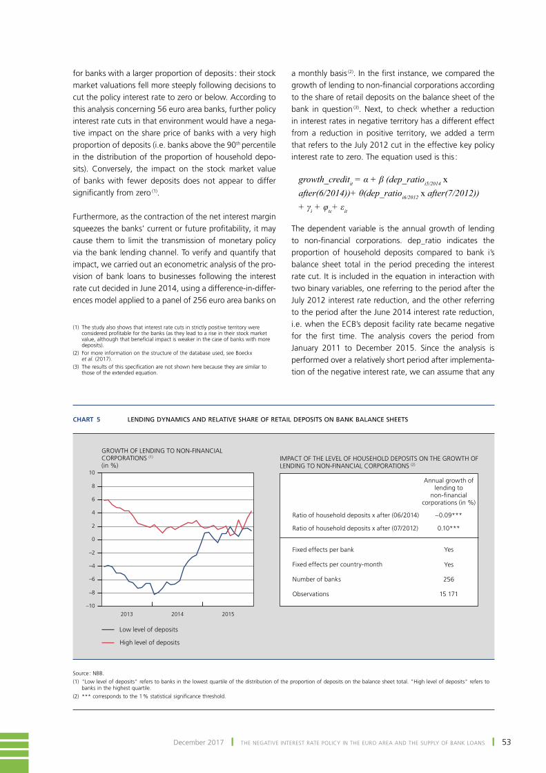
53December 2017 ❙ tHE NEgAtIvE INtERESt RAtE polIcY IN tHE EuRo AREA AND tHE SupplY of BANk loANS ❙
for banks with a larger proportion of deposits : their stock market valuations fell more steeply following decisions to cut the policy interest rate to zero or below. According to this analysis concerning 56 euro area banks, further policy interest rate cuts in that environment would have a nega‑tive impact on the share price of banks with a very high proportion of deposits (i.e. banks above the 90th percentile in the distribution of the proportion of household depo‑sits). Conversely, the impact on the stock market value of banks with fewer deposits does not appear to differ significantly from zero (1).
furthermore, as the contraction of the net interest margin squeezes the banks’ current or future profitability, it may cause them to limit the transmission of monetary policy via the bank lending channel. To verify and quantify that impact, we carried out an econometric analysis of the pro‑vision of bank loans to businesses following the interest rate cut decided in June 2014, using a difference-in-differ‑ences model applied to a panel of 256 euro area banks on
a monthly basis (2). In the first instance, we compared the growth of lending to non-financial corporations according to the share of retail deposits on the balance sheet of the bank in question (3). Next, to check whether a reduction in interest rates in negative territory has a different effect from a reduction in positive territory, we added a term that refers to the July 2012 cut in the effective key policy interest rate to zero. The equation used is this :
growth_creditit = α + β (dep_ratioi5/2014 x after(6/2014))+ θ(dep_ratioi6/2012 x after(7/2012)) + γi + φtc+ εit
The dependent variable is the annual growth of lending to non-financial corporations. dep_ratio indicates the proportion of household deposits compared to bank i’s balance sheet total in the period preceding the interest rate cut. It is included in the equation in interaction with two binary variables, one referring to the period after the July 2012 interest rate reduction, and the other referring to the period after the June 2014 interest rate reduction, i.e. when the ECB’s deposit facility rate became negative for the first time. The analysis covers the period from January 2011 to December 2015. Since the analysis is performed over a relatively short period after implementa‑tion of the negative interest rate, we can assume that any
(1) The study also shows that interest rate cuts in strictly positive territory were considered profitable for the banks (as they lead to a rise in their stock market value, although that beneficial impact is weaker in the case of banks with more deposits).
(2) for more information on the structure of the database used, see Boeckx et al. (2017).
(3) The results of this specification are not shown here because they are similar to those of the extended equation.
Chart 5 LENDING DYNAMICS AND RELATIVE SHARE OF RETAIL DEPOSITS ON BANK BALANCE SHEETS
2013 2014 2015
–10
–8
–6
–4
–2
0
2
4
6
8
10
Ratio of household deposits x after (06/2014)
Ratio of household deposits x after (07/2012)
Fixed effects per bank
Fixed effects per country-month
Number of banks
Observations
IMPACT OF THE LEVEL OF HOUSEHOLD DEPOSITS ON THE GROWTH OF LENDING TO NON-FINANCIAL CORPORATIONS (2)
Annual growth of lending to
non-financial corporations (in %)
–0.09***
0.10***
Yes
Yes
High level of deposits
Low level of deposits
256
15 171
GROWTH OF LENDING TO NON-FINANCIAL CORPORATIONS (1)
(in %)
Source : NBB.(1) "Low level of deposits" refers to banks in the lowest quartile of the distribution of the proportion of deposits on the balance sheet total. "High level of deposits" refers to
banks in the highest quartile.(2) *** corresponds to the 1 % statistical significance threshold.

54 ❙ tHE NEgAtIvE INtERESt RAtE polIcY IN tHE EuRo AREA AND tHE SupplY of BANk loANS ❙ NBB Economic Review
changes in the banks’ business model were fairly limited. In order to take account of the specific characteristics of the individual banks and the economic and financial situation at that time, we included fixed effects per bank and per country‑month.
The results show that a larger proportion of household deposits in relation to the assets implies a smaller increase in lending to non-financial corporations in the 18 months following the introduction of the negative interest rate. More specifically, each additional percentage point of household deposits (compared to the balance sheet to‑tal) causes a 9 basis point reduction in the year-on-year growth of lending to businesses. The impact of the July 2012 interest rate cut was the opposite, with a stronger rise in the growth of lending where household deposits formed a larger share of the balance sheet.
this conclusion is similar to that of Heider et al. (2017), who find that banks holding more deposits lend less to businesses after the implementation of a negative interest rate than banks with fewer deposits. They also find that the banks with a higher proportion of deposits concentrate their loans on riskier businesses : an increase in the ratio of deposits is associated with lending to busi‑nesses whose return on assets is relatively more volatile. unfortunately, our database does not enable us to analyse any possible effects on risk‑taking by banks.
the analyses presented here, based on difference‑in‑differences models, only reveal a relative effect resulting from comparison of the behaviour of individual banks. these models therefore do not indicate that the negative interest rate has any adverse effect – in absolute terms – on lending. Instead, they show that the greater the ratio of retail deposits on a bank’s balance sheet, the more slowly the bank’s lending will grow in relation to the average bank. that does not permit any conclusions regarding the effect of the negative interest rate on the average bank’s lending. Chart 5 shows that credit growth remained positive after the June 2014 interest rate cut, both for banks with a high ratio of deposits and for those with fewer deposits. However, section 5 will demonstrate that this is not necessarily due purely to the easing effect of the negative interest rate.
the impact of the volume of household deposits on banks’ profitability, and ultimately on lending, may also be influenced by the margin available to the banks for lowering the interest rate on their deposits at the time of the rate cut. That margin will determine how soon and to what degree the banks will have to contend with negative pressure on their net interest margin. However, we are not dealing with an absolute concept here : for
example, legal restrictions which vary from one country to another may impose different lower limits for certain deposit interest rates. that makes it very challenging to test this hypothesis.
4.2 composition and duration of bank assets
The economic lower bound of interest rates is also likely to depend on the composition and duration of banks’ as‑sets. It may be beneficial for the banks to hold assets with a longer duration, on which the interest income is less susceptible to interest rate changes. A portfolio of long‑term bonds or fixed-interest loans can guarantee the bank a stable interest income until the bonds or loans mature, implying that in the meantime they maintain a higher net interest margin (all other things being equal), since their funding costs are adjusted – albeit only partially – as a result of the interest rate cut.
In the case of loans, it is the rate fixation period rather than the loan duration that largely determines the speed of adjustment to the new level of interest rates. The reference rates for loans at variable interest are generally market interest rates which, as already mentioned, have responded strongly to the reductions in the policy interest rate, even in negative territory. This shows that variable-rate loans, and especially those on which the interest rate is revised after a relatively short time, can lead to a considerable loss of interest income on the banks’ existing portfolio.
The proportion of variable-rate loans varies greatly between the euro area countries, as each country has its own well-established practices or customs, especially as regards household mortgage loans. That disparity is reflected in dif‑ferences in the impact of key interest rate changes. Banks which mainly lend at fixed rates may also be affected by interest rate changes when refinancing the loans, although the effect is less automatic and systematic. However, if the refinancing process comes with a fee for the lender, the negative impact on the income of the bank concerned is partly mitigated (at least in the short term).
The volume and maturity of the fixed-income bonds in the portfolio of marketable securities also determine the sen‑sitivity of the bank’s profitability to the negative interest rate. thus, a larger proportion of bonds in the balance sheet total and a longer residual maturity are associated with a less detrimental impact on profitability, because the value of the securities held increases when the interest rate falls, and the rise is all the greater the longer their maturity. Conversely, if banks hold few bonds or have more short‑dated securities, the capital gains generated

55December 2017 ❙ tHE NEgAtIvE INtERESt RAtE polIcY IN tHE EuRo AREA AND tHE SupplY of BANk loANS ❙
by a reduction in interest rates will be smaller. Banks are then less able to offset future losses on their net interest margin if the change in their funding costs is only partial.
more generally, the proportion of marketable securities that banks hold seems to attenuate the adverse impact of the negative interest rate on the supply of loans to non‑financial corporations. If the same economic analysis as before is applied first to banks with a higher proportion of marketable assets (1) and then to those with a lower pro‑portion (the upper and lower quartiles of the distribution respectively), the results differ significantly. For banks with a large volume of marketable assets, the deposit ratio did not hamper the growth of lending to businesses in a period of negative interest rates (as the coefficient was considerably lower than for banks holding fewer negotiable assets, and was not significantly different from zero). In contrast, for banks with a small volume of marketable assets, the im‑pact of household deposits on growth escalates (–22 basis points as opposed to an average of –9 basis points). By attenuating the adverse effect of the negative interest rate on bank profitability, the rise in the value of securities also seems to temper its potential negative impact on lending.
In the end, the banks’ assets with the shortest maturity and the greatest sensitivity to interest rates are the excess liquidity that they deposit at the central bank in excess of their reserve requirements. A bank will incur losses on its excess reserves if the interest rate applied to them is lower than the marginal cost of their financing (Buiter and Rahbari, 2016). Although those losses are not confined to periods of negative interest rates, it is likely that, when the interest rate falls below zero, the marginal cost of funding will be relatively high for banks holding a large proportion of household deposits, owing to the rigidity of their remuneration. If banks hold a large volume of excess liquidity, that may therefore depress their interest income and – in the event of rigid funding costs – their profitabi-lity. However, there are several factors that influence the size of that impact.
First, although the weight of the excess liquidity in the balance sheet total of euro area banks has increased sub‑stantially since the beginning of 2015, it is still relatively low (6 % in August 2017), especially compared to the ratio of retail deposits (22 % on that same date). Thus, a reduction of less than 3 basis points in the household deposit interest rate would offset the loss of net interest income resulting from a 10 basis point reduction in the EcB deposit facility rate.
Chart 6 LENDING AT VARIABLE INTEREST RATES COMPARED TO LENDING AT FIXED RATES IN THE EURO AREA
0
10
20
30
40
50
60
70
80
90
2007 2009 2011 2013 2015 20170
1
2
3
4
5
6
7
DE BE FR NL EA EL LU IE AT IT ES PT FI
PROPORTION OF THE TOTAL OUTSTANDING LOANS TO HOUSEHOLDS AND NON-FINANCIAL CORPORATIONS GRANTED AT VARIABLE RATES IN MARCH 2014(in %)
INTEREST RATE ON OUTSTANDING LOANS TO HOUSEHOLDS AND NON-FINANCIAL CORPORATIONS (in %)
Countries where most loans are at variable rates
Countries where most loans are at fixed rates
Sources : ECB, own calculations.
(1) the sum of the debt instruments (issued by the public or the private sector, but other than by banks) and private sector shares (excluding banks) in proportion to the balance sheet total.

56 ❙ tHE NEgAtIvE INtERESt RAtE polIcY IN tHE EuRo AREA AND tHE SupplY of BANk loANS ❙ NBB Economic Review
Second, the strong rise in excess liquidity in recent years is the counterpart to the securities purchased by the Eurosystem under the App. In so far as those securities were held by the banks themselves, they generated capital gains for the banks when they were sold.
The third and final point is that the distribution of the excess liquidity between banks is an important factor for assessing the impact : if it is concentrated mainly on banks with a small ratio of retail deposits, the effect on the sector’s profitability should be very small (1).
4.3 Has the supply of bank loans suffered as a result of the negative interest rate ?
However, it must be said that neither the data so far nor the analyses mentioned here show any contractionary effect attributable to the negative interest rate in absolute terms, as defined by Brunnermeier and Koby (2017) (2). In general, the implementation of the nega‑tive interest rate policy in the euro area was accompa‑nied by an acceleration in lending and a steep decline in bank debit interest rates. Interest rates on loans fell by significantly more than the average reference interest rate on the interbank market (i.e. the rate at which banks can raise funding on that market) (ECB, 2017a). these positive developments are borne out by the banks’ answers to questions concerning the impact of the negative interest rate on lending, included in the quarterly bank lending survey in the euro area. Despite the adverse impact on net interest income, the nega‑tive interest rate seems to have had a positive impact on the volume of lending and helped to drive down debit interest rates (ECB, 2017c). At the same time, some euro area banks have focused more on activities generating fees and commissions in order to offset the fall in their net interest income (ECB, 2016b).
However, it is still difficult to identify the specific con‑tribution of the negative interest rate to the observed movement in debit interest rates and bank lending, as the EcB implemented other measures at the same time, such as forward guidance, asset purchase programmes, and targeted longer-term refinancing operations. The next section examines the interactions between the negative interest rate and those measures.
5. Interactions and complementarity between the negative interest rate policy and the other monetary policy measures
the effects and the transmission channels of the vari‑ous monetary policy measures adopted by the EcB since June 2014 interact and complement one another. The combination of those measures may therefore also have specific additional consequences for the banking sector’s profitability and for the transmission via the banks.
In general, the presence of a lower bound may inhibit the central bank’s ability to ease monetary policy fur‑ther (Goodfriend, 2016). The negative interest rate may therefore be regarded as a measure that reinforces the effect of both conventional and non‑standard monetary policy (Rostagno et al., 2016). Under conventional policy, reductions in the interest rate below zero may thus have a bigger impact on financial conditions than interest rate cuts in positive territory if they change the perception of the lower bound of key policy interest rates. In the context of the euro area, the negative interest rate thus amplified the effect of the forward guidance (Cœuré, 2016) : since interest rates are expected to remain low in the future, the reduction below zero in fact lowered future rate expecta‑tions, causing the rest of the yield curve – well beyond the short segment – to move downwards.
At the same time, some other EcB measures reinforce the effect on the yield curve of the interest rate cuts in nega‑tive territory, particularly the forward guidance and the asset purchase programme, the impact of which is more marked on the medium and long segments of the yield curve. Thus, apart from the downward shift caused by the interest rate cuts, the yield curve flattened out, and that may have varying effects on banks’ profitability. On the one hand, since the banks normally gain from a steeper yield curve, that may further dent their profitability, as the assets previously held are replaced with assets generating lower interest income, implying direct losses on the net interest margin unless the funding costs are adjusted to the same degree.
on the other hand, the simultaneous implementation of the various measures helps to reinforce the easing of financial conditions, and in so doing, to enhance the beneficial effect of the interest rate reduction on the euro area’s economy. Consequently, the aim of the measures – namely, to boost the economy and inflation – could be attained more quickly, thus reducing the period of time in which interest rates have to remain at very low levels, and hence the potentially adverse impact that a long period of negative interest rates may have on the banks.
(1) Baldo et al. (2017) show that the distribution of the liquidity depends partly on the banks' business models: investment banks and clearing institutions thus tend to accumulate more excess liquidity in relation to their balance sheet total. That suggests that excess liquidity does not present a risk for the transmission of monetary policy to bank lending.
(2) However, an analysis by Goldman Sachs Economic Research (Hazell and Pill, 2016) shows that the growth of lending to businesses declines following a reduction interest rates if those rates are at very low levels or below zero.
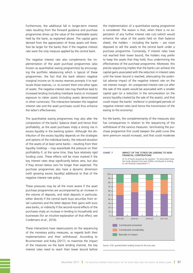
57December 2017 ❙ tHE NEgAtIvE INtERESt RAtE polIcY IN tHE EuRo AREA AND tHE SupplY of BANk loANS ❙
furthermore, the additional fall in longer‑term interest rates resulting from the forward guidance and purchase programmes drives up the value of the marketable assets held by the bank, as explained above. the capital gains derived from the appreciation of those assets will there‑fore be larger for the banks than if the negative interest rate were the only measure applied by the central bank.
the negative interest rate also complements the im‑plementation of the asset purchase programmes (also known as quantitative easing programmes) by encourag‑ing the portfolio rebalancing which is typical of these programmes : the fact that the bank obtains negative marginal income on its excess reserves prompts it to real‑locate those reserves, i.e. to convert them into other types of assets. the negative interest rate may therefore lead to increased lending (including interbank loans) or increased exposure to riskier assets (including assets denominated in other currencies). The interaction between the negative interest rate and the asset purchases could thus enhance the latter’s effectiveness.
The quantitative easing programmes may also alter the composition of the banks’ balance sheet and hence their profitability, as the asset purchases imply a strong rise in excess liquidity in the banking system. Although the dis‑tribution of the excess liquidity depends on the strategies and options of the individual banks, the reduced duration of the assets of at least some banks – resulting from their liquidity holdings – may exacerbate the pressure on their profitability if, at the same time, they face relatively rigid funding costs. These effects will be more marked if the key interest rates drop significantly below zero, but also if they remain below zero for longer than expected. The purchase programmes also have a dynamic dimension (with growing excess liquidity) additional to that of the negative interest rate policy.
these pressures may be all the more severe if the asset purchase programmes are accompanied by an increase in the volume of deposits, and retail deposits in particular, either directly if the central bank buys securities from re‑tail customers and the latter deposit their gains with euro area banks, or indirectly if the second‑round effects of the purchases imply an increase in lending to households and businesses (for an intuitive explanation of that effect, see cordemans et al., 2016).
These interactions have repercussions on the sequencing of the monetary policy measures, as regards both their implementation and their withdrawal. According to Brunnermeier and Koby (2017), to maximise the impact of the measures via the bank lending channel, the key interest rates need to reach their lower bound before
the implementation of a quantitative easing programme is considered. The reason is that, when there is no ex‑pectation of any further interest rate cuts (which would enhance the value of the assets held on their balance sheet), the holders – including the banks – are more disposed to sell the assets to the central bank under a purchase programme. conversely, if interest rates have not reached their lower bound, the holders may prefer to keep the assets that they hold, thus undermining the effectiveness of the purchase programme. moreover, this precise sequencing implies that the banks can achieve the capital gains associated with the reduction in interest rates until the lower bound is reached, attenuating the poten‑tial adverse impact of the negative interest rate on the net interest margin. An unexpected interest rate cut after the sale of the assets would be associated with a smaller capital gain (or a reduction in the remuneration on the excess liquidity created by the sale of the assets), and that could impair the banks’ resilience in prolonged periods of negative interest rates (and hence the transmission of the easing to the economy).
for the banks, the complementarity of the measures also has consequences in relation to the sequencing of the withdrawal of the various measures : terminating the pur‑chase programme first could steepen the yield curve (the term premium would increase), and that could moderate
Chart 7 IMPACT OF THE TLTROS ON LENDING TO NON-FINANCIAL CORPORATIONS
(in % of banks answering the question "To what extent have the funds obtained from past tltRos contributed to lending to non-financial corporations ?")
0
10
20
30
40
50
60
70
80
90
100
Contributed somewhat
Contributed considerably
Basically no impact
2015-Q3 2016-Q1 2016-Q3 2017-Q1
Source : ECB, quarterly Bank Lending Survey for the euro area.

58 ❙ tHE NEgAtIvE INtERESt RAtE polIcY IN tHE EuRo AREA AND tHE SupplY of BANk loANS ❙ NBB Economic Review
the potentially negative impact of a prolonged period of negative interest rates on the banks’ profitability, while keeping short-term interest rates at relatively low levels.
The complementarity between the negative interest rate and the TLTROs is more specific and more bank-centred. These operations, which aim to encourage bank lending to businesses, provide very cheap medium‑term funding for the participating banks (1) : they thus exert downward pressure on the banks’ funding costs (both directly, for those borrowing funds, and indirectly, by offering an additional source of funding competing with traditional sources such as bank bond issuance or interbank loans, and driving down their yields). More particularly, the second series of tltRos implemented since June 2016 offers funds for a period of up to four years at an interest rate potentially equal to the deposit facility rate. In October 2017, the liquidity created by the TLTROs amounted to € 758 billion, or 42 % of the excess liquidity in the euro area’s banking system, and 2.4 % of the banks’ balance sheet total.
By reducing the banks’ funding costs, the tltRos attenu‑ated the negative impact of the rigidity of deposit interest rates on the banks’ net interest margin, and therefore on lending. According to the responses of the quarterly bank lending survey in the euro area, the banks consider that the TLTROs boosted lending to non-financial corporations.
conclusion
In recent years, the negative interest rate policy, together with other non-standard monetary policy measures, has become an additional tool for central banks. Although its use is widespread, both to combat deflationary risks and (1) For more information on the TLTROs, see for instance ECB (2017d).
to control exchange rates, it has its limitations as regards monetary transmission via the banks.
Those limitations are due to the existence of a lower bound at around 0 % for retail deposit interest rates. This lower bound implies downward rigidity of the banks’ funding costs once the key interest rate has fallen too low, and especially if it drops below zero.
The downward rigidity of the banks’ funding costs may create downward pressure on their net interest margin, and ultimately constrain their ability to lend more to the economy. Also, the longer the period of negative interest rates, the greater the likelihood of contractionary effects on lending dynamics. However, the banks may also benefit from capital gains and the improvement in the macroeconomic conditions associated with monetary easing. thus, the ultimate effect of the negative interest rate on the banks’ profitability and on their lending will depend on the composition of the banks’ balance sheet.
furthermore, the negative interest rate policy in the euro area is not an isolated measure. the interactions and the effects of complementarity with other monetary policy measures may attenuate the potentially restrictive effect of a negative interest rate policy on the banks’ profitabi-lity and on their capacity to lend more. the combination of measures may also facilitate transmission, helping to achieve the monetary policy objectives more quickly and limit the length of time for which the negative interest rate is necessary. Developments in lending in the euro area since the implementation of the negative interest rate policy seem to indicate a smooth transmission via the banks.

59December 2017 ❙ tHE NEgAtIvE INtERESt RAtE polIcY IN tHE EuRo AREA AND tHE SupplY of BANk loANS ❙
Bibliography
Altavilla C., G. Carboni and R. Motto (2015), Asset Purchase Programmes and Financial Markets : Lessons from the Euro Area, EcB, Working paper Series 1864.
Ampudia M. and S. Van den Heuvel (2017), Monetary policy and bank equity values in a time of low interest rates (in preparation / October 2017 version ; SSRN : https : / / papers.ssrn.com / sol3 / papers.cfm ? abstract_id=2976372).
Arteta C., M. A. Kose, M. Stocker and T. Taskin (2016), Negative Interest Rate Policies : Sources and Implications, World Bank group, policy Research Working paper 7791.
Baldo l., B. Hallinger, c. Helmus, N. Herrala, D. martins, f. mohing, f. petroulakis, m. Resinek, o. Bergote, B. usciati and Y. Wang (2017), The distribution of excess liquidity in the euro area, EcB, occasional paper Series 200.
Barr M., B. Kasman and D. Mackie (2016), Negative Policy Rates : The Bound Is Lower Than You Think, j.p. morgan, Special Report, Economic Research, 9 February.
Bech M. and Malkhozov A. (2016), "How have central banks implemented negative policy rates ?", BIS Quarterly Review, March, 31-44.
Bernanke S. and M. Gertler (1995), "Inside the Black Box : The Credit Channel of Monetary Policy Transmission", Journal of Economic Perspectives, 9(4), 27-48.
Bindseil U. (2017), Negative interest rates and (other) non-conventional measures – Motivation and ECB experience, Presentation at the IMF-BoA conference on negative euro area rates, Tirana, Albania, 5 May.
Boeckx J., M. de Sola Perea and G. Peersman (2017), The Transmission Mechanism of Credit Support Policies in the Euro Area, cESifo Working paper Series 6442.
Borio C., L. Gambacorta and B. Hofmann (2015), The influence of monetary policy on bank profitability, BIS Working papers No. 514, october.
Borio C. and A. Zabai (2016), Unconventional monetary policies : a re-appraisal, BIS Working papers No. 570, july.
Brunnermeier M.K. and Y. Koby (2017), The Reversal Interest Rate : The Effective Lower Bound of Monetary Policy (in prep‑aration / July 2017 version ; https : / / scholar.princeton.edu / markus / publications / reversal-interest-rate-effective-lower- bound-monetary-policy).
Buiter, W. H. (2009), Negative Nominal Interest Rates : Three Ways to Overcome the Zero Lower Bound, NBER, Working paper 15118.
Buiter, W.H. and N. Panigirtzoglou (2003), "Overcoming the Zero Bound on Nominal Interest Rates with Negative Interest on Currency : Gesell’s Solution", Economic Journal, 113(490), 723-46.
Buiter, W.H. and E. Rahbari (2016), How Many Financial Sector Business Models Are Damaged By Low and Negative Rates ?, Citi Research, Global Economics Review, 20 June.
Claessens, S., N. Coleman and M. l. Donnelly (2017), Low-For-Long Interest Rates and Banks’ Interest Margins and Profitability : Cross-Country Evidence, International finance Discussion papers 1197.
Cœuré B. (2014), Life below zero : Learning about negative interest rates, Speech at the annual dinner of the EcB’s Money Market Contact Group, Frankfurt, Germany, 9 September.

60 ❙ tHE NEgAtIvE INtERESt RAtE polIcY IN tHE EuRo AREA AND tHE SupplY of BANk loANS ❙ NBB Economic Review
Cœuré B. (2016), Assessing the implications of negative interest rates, Speech at the Yale Financial Crisis Forum, New Haven, USA, 28 July.
Cordemans, N., M. Deroose, M. Kasongo Kashama and A. Stevens (2016), "The ABC of quantitative easing – Or the basics of asset purchases by central banks", NBB, Economic Review, June, 33-47.
De Backer B. and J. Wauters (2017), "The cyclical and structural determinants of the low interest rate environment", NBB, Economic Review, September, 73-92.
Deroose M. and A. Stevens (2017), "Low inflation in the euro area : causes and consequences", NBB, Economic Review, June, 117-134.
ECB (2016a), "Trends in the external financing structure of euro area non-financial corporations", Economic Bulletin, Issue 5, 29-32.
ECB (2016b), "Adapting bank business models : financial stability implications of greater reliance on fee and commission income", Financial Stability Review, November, 147‑157.
ECB (2017a), "MFI lending rates : pass-through in the time of non-standard monetary policy", Economic Bulletin, Issue 1, 40-63.
ECB (2017b), Sensitivity Analysis of IRRBB – Stress test 2017 Final results, october.
ECB (2017c), The euro area bank lending survey. Third quarter of 2017, october.
ECB (2017d), "The targeted longer-term refinancing operations : an overview of the take-up and their impact on bank intermediation", Economic Bulletin, Issue 3, 42-46.
Eser F., M. C. Amaro, S. Iacobelli and M. Rubens (2017), The use of the Eurosystem’s monetary policy instruments and operational framework since 2012, EcB, occasional paper Series 188.
IMF (2016), "Article IV Consultation, Euro Area Policies : Selected Issues Paper", Country Report, 16 / 220.
IMF (2017), Negative interest rate policies – Initial experiences and assessments, policy paper.
Genay H. and R. Podjasek (2014), What is the Impact of Low Interest Rate Environment on Bank Profitability ?, federal Reserve Bank of Chicago, Chicago Fed Letter 324.
Goodfriend, M. (2000), "Overcoming the Zero Bound on Interest Rate Policy", Journal of Money, Credit, and Banking, 32(4), Part 2, 1007-35.
Goodfriend, M (2016), The case for unencumbering interest rate policy at the zero lower bound, jackson Hole Economic Policy Symposium, Federal Reserve Bank of Kansas City, Jackson Hole, Wyoming, 26-27 August.
Hazell J. and H. Pill (2016), Monetary policy transmission : When rates are (very) low, the bank lending channel is weak, European Economic Analyst, Goldman Sachs Economic Research, 15 September.
Heider F., F. Saidi and G. Schepens (2017), Life Below Zero : Bank Lending Under Negative Policy Rates (SSRN : htt‑ps : / / ssrn.com / abstract=2788204).
Jobst A. and H. Lin (2016), Negative Interest Rate Policy (NIRP) : Implications for Monetary Transmission and Bank Profitability in the Euro Area, Imf, Working paper 16 / 172.

61December 2017 ❙ tHE NEgAtIvE INtERESt RAtE polIcY IN tHE EuRo AREA AND tHE SupplY of BANk loANS ❙
Kasongo Kashama M. (2014), "The how and why of a negative interest rate for the deposit facility", NBB, Economic Review, September, 107‑116.
Kimball M. (2013), How and Why to Eliminate the Zero Lower Bound : A Reader’s Guide, confessions of a Supply‑Side Liberal blog, 20 September.
Madashi C. and I. P. Nuevo (2017), The profitability of banks in a context of negative monetary policy rates : the cases of Sweden and Denmark, EcB, occasional paper Series 195.
McAndrews J. (2015), Negative Nominal Central Bank Policy Rates : Where Is the Lower Bound ?, Speech at the university of Wisconsin, Madison, USA, 8 May.
Panigirtzoglou N., N.Srivastava, J. Vakharia and M. Inkinen (2016), The unintended consequences of very negative rates, J.P. Morgan, Flows & Liquidity, Economic Research, 12 February.
Rahbari E., W. H. Buiter and C. Rojas (2016), Negative Policy Rates – What’s Next ? Who’s Next ?, citi Research, global Economics Review, 11 February.
Rogoff K. (2014), Costs and Benefits of Phasing Out Paper Currency, paper presented at the NBER macroeconomics Annual Conference, Harvard University, Massachusetts, USA, 11 April.
Rostagno M., U. Bindseil, A. Kamps, W. Lemke, T. Sugo and T. Vlassopoulos (2016), Breaking through the zero line. The ECB’s negative interest rate policy, Presentation at the Brookings Institution Conference on negative interest rates : Lessons learned… so far, Washington DC, USA, 6 June.
Woodford M. (2012), Methods of Policy Accommodation at the Interest-Rate Lower Bound, proceedings – Economic policy Symposium – jackson Hole, federal Reserve of kansas city, 185‑288.

63December 2017 ❙ toWARDS A NEW polIcY mIX IN tHE EuRo AREA ? ❙
Towards a new policy mix in the euro area ?
P. ButzenS. ChelioutN. CordemansE. De PrestW. MelynL. Van MeenselS. Van Parys
Introduction
Aiming for stable, non-inflationary economic growth that promotes full employment, macroeconomic policy has a crucial stabilising role to play in market econo‑mies. The recent global economic and financial crisis has not fundamentally challenged the existing con‑sensus, but merely brought into relief some of its weaknesses. Besides, in the current economic climate of moderate growth, subdued inflation and low inter‑est rates, monetary and fiscal policies need revisiting in terms of both their purpose and their functioning. The euro area is subject to highly specific conditions, as it has also pulled through a very instructive sovereign debt crisis.
This is the setting for this article’s incisive review of the macroeconomic policy mix in the euro area. Its first section discusses the pre-crisis macroeconomic consensus as well as lessons learned from the crisis. Section 2 summarises today’s macroeconomic situa‑tion and the third section the Eurosystem’s monetary policy framework. The fourth section investigates what would be the most appropriate fiscal policy in the cur‑rent circumstances, both in individual countries and in the euro area as a whole. Section 5 looks more closely at Germany’s specific role. The sixth section addresses the question of whether there is any need for a revised European policy framework, and the article ends on a number of conclusions.
1. The policy mix : fresh insights
1.1 the macroeconomic consensus prior to the financial crisis
market economies are intrinsically prone to economic cy‑cles, i.e. times of economic expansion and contraction, the length of which varies. The frequency and duration of such periods depend on random events of a varied nature, known as “shocks” in economic speak, including technological, financial or other innovations, geopolitical developments, weather conditions, public policy changes or even “animal spirits” (Keynes, 1936 ; Akerlof and Schiller, 2009). Such ani‑mal spirits are part and parcel of human nature and reflect upbeat or gloomy expectations influencing decisions made by economic agents.
The financial sector accelerates economic cycles (Bernanke et al., 1996), as lending for consumption or capital spend‑ing is typically underpinned by collateral and / or security. the values of such collateral tend to rise at times of opti‑mism and economic expansion, fostering credit allocation and supporting spending. conversely, collateral loses value when gloom sets in and economic activity con‑tracts. then, credit becomes scarcer and consumption and capital spending are squeezed. Even ignoring the wealth effect, which reflects the wealth impact of changes in consumption and savings, this interaction between the financial and real spheres of the economy can prompt, as

64 ❙ toWARDS A NEW polIcY mIX IN tHE EuRo AREA ? ❙ NBB Economic Review
the case may be, virtuous or vicious circles of economic expansion or contraction.
the variability of economic activity creates uncertainty and weighs on consumption and investment decisions, given that individuals are risk averse. What is more, economic activity typically also involves variable inflation and em‑ployment, entailing steep welfare costs. Unstable inflation depresses confidence and consumer purchasing power, while inflating risk premiums in the financial markets and causing interest rates to rise. As such, it makes it harder to take economic decisions and gets in the way of an optimal allocation of resources. unpredictable price level variability eventually results in a random redistribution of wealth and income between debtors and creditors, with the extreme case of a deflationary spiral – in which lower prices push up debt and the reverse – being particularly pernicious (see Fisher, 1933). Growing unemployment when economic activity slows does not just cause income losses, it also spells a loss in human capital.
Against this background, macroeconomic policy focuses on preventing and keeping to a minimum the undesirable effects of economic vicissitudes : as the consensus that has emerged since the early 1980s would have it, macroeco‑nomic policy should encourage stable, non-inflationary economic growth promoting full employment. Monetary and fiscal policies are two key instruments to help achieve this state of affairs.
Monetary policy ensures price stability
monetary policy regulates a country’s money supply and / or the price of money in the economy – with “mon‑ey” defined as the total means of payment – and aims to ensure price stability in the medium term, its best possible contribution to economic prosperity and job creation. Working on the principle of “divine coincidence”, a coun‑try’s central bank controls the output gap, i.e. the differ‑ence between real and potential production, by keeping
a close rein on inflation (Blanchard and Galí, 2007). This also promotes full employment.
The emphasis on the medium term is justified by the time lags in monetary policy transmission and the desire to keep to a minimum any output swings caused by exces‑sively active central bank behaviour. to eliminate any in‑flation bias, it is advisable to entrust monetary policy to a central bank independent of a country’s government, and to rule out any monetary financing of government debt.
Incidentally, price stability typically contributes to financial stability. By keeping at bay excessive inflation, it restricts the risks of contracts agreed in nominal terms, and, by warding off deflation, it prevents an increase in debt in real terms (Aucremanne and Ide, 2010). A central bank should keep an eye on trends in asset prices, but only in as much as price stability comes under threat. And it also acts as lender of last resort, stepping in with urgently needed cash when financial panic hits (1).
key policy rates are the traditional monetary policy instru‑ment of choice, used by central banks to steer money market rates and so influence financing conditions in the economy at large. monetary authorities implicitly observe the Taylor rule (Taylor, 1993) by responding to deviations in inflation from its targets and to deviations in output growth relative to its potential levels. To make an impact on real interest rates, which are deemed relevant to con‑sumption and investment decisions, the authorities adjust key policy rates more than proportionally so as to allow for variations in inflation.
Fiscal policy underpinned by automatic stabilisers
fiscal policy regulates government revenue and expendi‑ture in the economy and contributes to macroeconomic stabilisation chiefly through automatic stabilising mecha‑nisms. key stabilisers include taxes and social security benefits, as these of course smooth out fluctuations in economic activity.
In normal times – i.e. in a standard recession of relatively short length (2) – discretionary fiscal policy is not really the best way to go. In the real world, institutional limits and implementation delays reduce its efficacy and can even turn it procyclical. Besides, doubts arise over its implications due to uncertainties over the fiscal multiplier and potential Ricardian equivalence effects (3) (Blanchard et al., 2010). A final argument against discretionary fiscal policy is the leading role monetary policy is assigned to achieve macroeconomic stabilisation, obviating any sec‑ond instrument (4). And so, fiscal policy should exclusively focus on keeping public finances sustainable without
(1) This role was at the very heart of the inception of many central banks in the 19th and 20th centuries. In this capacity, they served both the banking industry and government, as both are closely linked and immediately exposed to default risks in the event of a crisis of confidence. Since these happen very rarely in the real world, central banks’ role as lender of last resort had become a dim memory in the advanced economies on the eve of the great recession.
(2) There is no consensus about a precise definition of a recession. America’s National Bureau of Economic Research (NBER) defines a recession as a significant decline in economic activity spread across the economy and lasting two or more quarters. Historically, recessions typically last about one year and involve a drop in production of less than 5%. If economic activity contracts more deeply and lasts longer, this may be referred to as a depression.
(3) This hypothesis suggests that the private sector will start saving more in response to fiscal expansion and higher government deficits, as firms and households assume that the government will raise taxes or cut benefits in the future. In its most extreme form, this theory implies that fiscal expansion does not boost the economy at all, just as fiscal contraction does not slow it down.
(4) This view has gained wide currency in academic circles and with central banks, but real-life discretionary measures are known to have been taken during “standard recessions” (Blanchard et al., 2010).

65December 2017 ❙ toWARDS A NEW polIcY mIX IN tHE EuRo AREA ? ❙
disrupting monetary policy in its essential task of ensuring price stability.
Many – though not all – agree that discretionary fiscal policy may have a stabilising macroeconomic role to play in the event of a liquidity trap (Keynes, 1936 ). A liquidity trap emerges after a major shock and when monetary policy can no longer boost prices or economic activity, as economic agents no longer respond to more abundant liquidity or key policy rates have hit bottom. Under these conditions, the fiscal multiplier is particularly high as the crowding-out effect (1) evaporates. this type of recession, incidentally, tends to persist beyond the time required for political decision‑making.
After the Great Depression of the 1930s, the liquidity trap was for a long time an intellectual oddity only found in school books. But japan’s experience from the mid‑1990s and the recession in the united States in the early 2000s sparked renewed interest in the subject (see Auerbach and Obstfeld, 2003 ; Eggertsson and Woodford, 2004).
The great moderation
By the mid-2000s, the framework described above was generally believed to have contributed to greater macro‑economic stability in the advanced economies. more stable economic growth and inflation, coupled with more moderate trends, had started in the early 1980s, a phenomenon referred to as the great moderation (see Bernanke, 2004).
Euro area : a consensus-matching framework
Based on the 1992 Maastricht Treaty, the institutional framework of the Economic and Monetary Union (EMU) largely reflected the pre-crisis macroeconomic consensus.
The common monetary policy was entrusted to an in‑dependent authority, the Eurosystem, whose mandate focuses on price stability. the EcB governing council’s monetary policy strategy specifies an inflation target for the euro area of “below, but close to, 2 % over the me‑dium term”. In normal times, the Eurosystem will tighten or relax its monetary policy stance by adjusting key policy rates up or down.
fiscal policy, by contrast, remained decentralised and the domain of national governments. that said, common rules apply, informed by the notion that governments should aim for fiscal equilibrium and give automatic stabi‑lisers free rein to cushion any shocks. Agreed in 1997, the Stability and Growth Pact (SGP) builds on the provisions in the maastricht treaty to impose maximum reference val‑ues for budget deficits and government debt (respectively, 3 % and 60 % of GDP) (2). Breaking down into a preventive and corrective arm, the pact is designed to ensure that countries in the EMU observe fiscal discipline, resulting in
Chart 1 DEVELOPMENTS AND VOLATILITY OF GDP GROWTH AND INFLATION IN ADVANCED ECONOMIES
1980
1982
1984
1986
1988
1990
1992
1994
1996
1998
2000
2002
2004
2006
–1
0
1
2
3
4
5
6
1980
1982
1984
1986
1988
1990
1992
1994
1996
1998
2000
2002
2004
2006
0
2
4
6
8
10
12
14
–0.5
0.0
0.5
1.0
1.5
2.0
2.5
3.0
0.0
0.5
1.0
1.5
2.0
2.5
3.0
3.5
Volatility of GDP growth (left-hand scale) Volatility of inflation (left-hand scale)
Inflation (right-hand scale)GDP growth (right-hand scale)
Source : IMF.
(1) A drop in private spending caused by the upward pressure on interest rates resulting from expansive fiscal policies.
(2) The nominal public deficit must not exceed 3 % of GDP, unless the deficit is declining considerably and continuously and is approaching the reference value, or unless the excess is exceptional and temporary and the deficit remains close to the reference value. the outstanding public debt must not exceed 60 % of GDP, or if it does so, it must approach that reference value at a satisfactory pace.

66 ❙ toWARDS A NEW polIcY mIX IN tHE EuRo AREA ? ❙ NBB Economic Review
improved coordination of policy measures, the soundness of public finances and prevention of spillover effects (1).
To ensure market discipline in addition to the fiscal-rules-based discipline, the treaty on the functioning of the European Union (TFEU) prohibits monetary financing of government debt (Article 123) and includes a “no-bail-out clause” (Article 125). The clause prohibits the European union and its member States from guaranteeing the com‑mitments of governments of other member States.
to give national governments an opportunity to respond more swiftly to idiosyncratic economic shocks despite a single monetary and currency policy, fiscal rules were re‑laxed slightly from 2005 on (2). Supranationally, however, the European institutional framework did not include a stabilising instrument – e.g. a lender of last resort or budgetary power.
1.2 lessons from the crisis
The 2007-10 global economic and financial crisis failed to produce a deep questioning of the prevailing general macroeconomic policy framework. There is no argument about its main planks of price stability and central bank independence. The sustainability of public finances has, for its part, received greater attention. that being said, the crisis did show up various weaknesses in the macro‑economic framework and, in the euro area, shone a stark light on the Emu’s incomplete institutional architecture in terms of supervision and assistance, which went fur‑ther than the flaws in the European budget framework (De Grauwe, 2013 ; Buti, 2016).
Macroeconomic framework : shortcomings
The first post-crisis finding is that price stability is a neces‑sary, but not a sufficient precondition for financial stability. greater macroeconomic stability during the “great moder‑ation” years has not prevented the emergence of financial imbalances : financial bubbles and property bubbles, exces‑sive debt of households and financial companies, etc. In fact, by putting downward pressure on interest rates, price stability may in fact have fuelled these developments as it created the conditions for riskier behaviour (Boeckx and Cordemans, 2017). The great recession also demonstrated the consequences of financial instability for monetary policy transmission and the real economy.
In fact, it became plain as day that macroprudential policy needed to take on board the stability of the financial system as a whole and prevent an accumulation of finan‑cial risks. many countries have introduced institutional
arrangements and tools to address the issue (IMF, 2016). Back on the agenda was the question of whether mon‑etary policy implementation should factor in risks to financial stability, although the debate has not yet been settled (see IMF, 2015).
Secondly, the financial crisis has also refocused minds on central banks’ crucial role as lender of last resort when liquidity in the markets dries up. It made abundantly clear that fiscal authorities in sovereign economies enjoy an implicit warranty in the monetary arena, as it is generally agreed that the sovereign debt crisis was exacerbated by the Eurosystem’s inability to take on the role of lender of last resort for euro area governments (Draghi, 2014).
In addition, the crisis threw into stark relief a third aspect : the limits to conventional monetary policies based on adjusting key policy rates. To ensure financial intermedia‑tion and solid monetary policy transmission, central banks have responded to the crisis by changing the make‑up of their balance sheets through qualitative easing. What’s more, central banks have relaxed their monetary policy even further by providing forward guidance on expected future developments in monetary policy. the crisis has also been instrumental in central banks mass‑buying of low-risk assets, a policy known as quantitative easing (see cordemans et al., 2016).
A fourth lesson taught by the crisis is that fiscal policy acts as a stabilising factor in a liquidity trap (3). this has been particularly visible in the united States and the united Kingdom, whereas euro area fiscal policy was more re‑stricted by the sovereign debt crisis (see below). Despite their delayed implementation, expansionary discretionary policies were also pursued in various countries due to the seriousness of the recession, its length and the constraints on monetary policy. Besides, fiscal multipliers were agreed to be higher – and positive – whenever key policy rates hit bottom (Eggertsson, 2011), meaning that higher govern‑ment spending translated into a higher than proportional increase in production in the economy. The financial crisis
(1) Specifically, any upward effects on euro area interest rates and inflation if caused by too expansive a fiscal policy. The temptation to pursue expansive fiscal policies is greater within a monetary union, as the central bank makes its monetary policy decisions based on average inflation. A country not pursuing sound fiscal policies could potentially benefit from lower real rates to boost its growth in the short term (Boeckx and Deroose, 2016).
(2) SGP requirements were generally eased. The emphasis was on strengthening the economic fundamentals and on the Pact’s flexibility. The reform modified both the preventive and the corrective arms. the main change to the preventive arm concerned the definition of the medium-term objective namely of a budget close to balance or in surplus. That objective was now expressed in structural terms, i.e. excluding the effects of the business cycle and one‑off factors. As for the Pact’s corrective procedures, there was significant easing of the definition of the exceptional circumstances in which a public deficit of over 3 % of GDP is not considered excessive.
(3) Some (Feldstein, 2016) even prefer addressing serious crises through fiscal rather than monetary policies. Arguably, fiscal policies do not entail the same risks to financial stability that attend some ‘unconventional’ monetary policy measures. By depressing risk‑free long rates, asset purchase programmes are said to encourage the search for yield and have a negative effect on bank profitability as they cause intermediation margins to shrink.

67December 2017 ❙ toWARDS A NEW polIcY mIX IN tHE EuRo AREA ? ❙
underlined how important it is to have fiscal room for ma‑noeuvre to address negative shocks, implying that debts should be reduced when business cycles are favourable.
lastly, the crisis has served to highlight potential interac‑tions between the two macroeconomic policy pillars. At times of recession, central banks use the monetary policy instrument to support the sustainability of public finances by easing financing conditions in the economy and by deploying asset purchase plans that typically focus on government paper. monetary policy, then, encourages fiscal recovery and the adoption of structural reforms. fiscal policy, in its turn, underpins price stability by sup‑porting aggregate demand. together, public spending and structural reforms contribute to potential growth and improve the efficiency of monetary policy by supporting real equilibrium interest rates (1).
Euro area construction defects
Membership of a monetary union potentially requires greater fiscal activism to stabilise national economies in the event of idiosyncratic shocks. the sovereign debt crisis that shook the euro area between early 2010 and the end of 2012 showed up major restrictions on national fiscal policy’s stabilising capability related to monetary union membership. Euro area member States contract debt obligations in a currency they have no control over : the fact that the Eurosystem is prohibited from engaging in monetary financing, coupled with the no-bail-out clause, makes them completely dependent on the financial mar‑kets and on market rules for funding. However, markets can be volatile and irrational, at times veering sharply away from macroeconomic fundamentals. This makes euro area countries extremely vulnerable to liquidity crises, which can easily degenerate into solvency crises.
Pressured by the markets and in the absence of adequate institutional euro area structures, some hard‑hit countries found themselves forced to adopt policies that were ex‑cessively restrictive and procyclical from a macroeconomic perspective (Orphanides, 2017). Their macroeconomic policy mix was dominated by the area’s common mon‑etary policy, which itself faced the lower bound of key policy rates (cordemans et al., 2016). This imbalance proved less than beneficial to both Member States and the euro area as a whole. De Grauwe (2013) argues that the monetary union as it was designed may well have exacerbated idiosyncratic shocks : countries hit the hard‑est plunged into a deflationary spiral.
The sovereign debt crisis also drew attention to the dis‑astrous consequences of banking sector troubles, as it weighs in heavily in the funding of the euro area economy
and the close ties between the industry and the govern‑ment sectors. The negative feedback loops between domestic sectors and government have caused financial markets to fracture along national lines and severely disrupted monetary policy transmission in the countries hardest hit. In the euro area, then, the crisis highlighted the implicit financial debt associated with the crucial role governments played in saving their countries’ banks (2).
lastly, the crisis in the euro area also underlined the importance of closer supervision of macroeconomic and financial imbalances, such as the property and credit bub‑bles that fed the troubles in the banking sector in various countries.
Government response
A range of measures proved crucial in addressing euro area shortcomings and their detrimental macroeconomic effects. first off, macroeconomic supervision and coordi‑nation of economic and fiscal policies in the EU were en‑hanced : the rules of the Stability and Growth Pact (SGP) (3)
were reviewed and supervision of imbalances was ex‑panded to other macroeconomic indicators than just pub‑lic finances, along with the introduction of the European Semester (4) and the treaty on Stability, coordination and Governance (TSCG) (5), etc.
A second set of measures was the introduction of Europe’s “firewalls” : the European Financial Stability Facility (EFSF) and the European financial Stabilisation mechanism (EFSM), followed by the European Stability Mechanism (ESM). This latter mechanism replaced the previous two in 2012 and led to the creation of an international finan‑cial institution authorised to raise money in the financial markets, so that the total emergency funding capacity reached € 700 billion. These resources may, under strict conditions, be drawn on to aid countries in need and rescue banks. Countries receiving such assistance were
(1) Real equilibrium rates pertain to interest rates that would apply in a normal output environment – i.e. when production matches its potential level – and that are in keeping with price stability. This theoretical rate is not constant over time and will change due to real factors that are a priori exogenous to monetary policy, e.g. an economy’s productivity. monetary policies are measured by the difference between real – i.e. adjusted for inflation – policy rates and real equilibrium rates (Boeckx et al., 2013).
(2) On the very eve of the crisis, various Member States subsequently most exposed to tensions had debt ratios that were not considered a problem. In 2008, Spain and Ireland, for instance, were looking at public debt as a percentage of GDP at around 40%. Setbacks in their banking sectors quickly deteriorated general government accounts.
(3) During the period running from 2011 to 2013, several reforms that widened and tightened up the European fiscal framework (Six Pack, Two Pack, Fiscal Compact) were approved. In 2015, however, the fiscal framework was relaxed as account is taken of the economic circumstances in the Member States when defining the efforts to be made under the preventive arm. for a detailed description of these reforms, see melyn et al. (2015).
(4) Annual cycle for the follow-up of and supervision of the economic policies of the European union and its member States.
(5) The TSCG – and the fiscal compact that is part of this Treaty – is an intergovernmental agreement between 25 EU Member States fostering convergence on the basis of strict rules. the treaty strengthens the implementation of the Sgp and enhances the supervision and coordination of economic policy.

68 ❙ toWARDS A NEW polIcY mIX IN tHE EuRo AREA ? ❙ NBB Economic Review
required to accelerate budget adjustments, but these would have likely been even more painful without such aid (Bénassy‑Quéré et al., 2016).
thirdly, the Eurosystem took on the role of lender of last resort for euro area governments. the governing council announced outright monetary transactions (OMTs) in the summer of 2012 and committed to buying, under certain conditions, unlimited amounts of government paper by way of these transactions, in response to the major and rapid deterioration of financing conditions in various Member States. These funding issues were not justified by the underlying macroeconomic and financial fundamentals, but they might have caused countries to crash out of the euro area and even threatened its very existence.
A fourth decision dating from 2012 was the creation of a banking union to break the negative spiral between national banking industries and their governments. As it stands, the banking union currently has two elements in place : a single supervisory mechanism (SSM) and a single resolution mechanism (SRM). The SSM provides uniform supervision of the euro area’s largest banks and is directed at a European level. the SRm’s objective is to resolve bankruptcies of troubled banks in an orderly manner, at the lowest possible cost to taxpayers (1) and the real economy. A third essential element of the new banking union, the European Deposit Insurance Scheme (EDIS), has yet to be created. Although the rules have been harmonised and despite the arguments in favour of a joint scheme (see Wolff, 2016), risk-sharing remains a very sensitive issue. for much the same reason, the resolution fund created to help banks in trouble is not backed by a supranational fiscal safety net.
finally, the European commission has proposed the es‑tablishment of a Capital Markets Union by 2019, with the general aim of bolstering the resilience of the European financial system. Integrating capital markets should en‑courage cross‑border risk‑sharing in the private sector and enhance funding and investment opportunities for both borrowers and savers.
taken together, these elements have steadily helped bring an end to the sovereign debt crisis from the summer of 2012, have facilitated more gradual adjustment and encouraged the economic recovery that got underway in 2013. Although the crisis has now run its course, the key question today is whether these measures taken to
prevent crises and absorb future shocks are indeed ad‑equate and sufficient.
Despite its increased flexibility, the Stability and Growth Pact still emphasises the sustainability of public finances and remains asymmetrical : countries exceeding their objectives are allowed to, but do not have to, boost their economies, with the pressure of adjustment invariably falling on deficit countries. What is more, the pact es‑pouses a strictly national approach, and fiscal policy for the Economic and Monetary Union as a whole is basically the sum of national policy measures. Some (for instance, De Grauwe, 2013) argue that this causes a deflationary distortion for the entire euro area.
many agree that the best possible macroeconomic sta‑bilisation, both at national and aggregate level, would require common fiscal capacity. Ever closer political union and budget integration would appear to guarantee the stability and continued existence of the monetary union. However, a stronger union raises important questions about democratic legitimacy. Any significant transfer of fiscal powers to the European level remains illusory at this stage.
2. macroeconomic situation today
Towards the end of 2012, the euro area embarked on an economic upturn on the back of a clear easing of the financial tensions caused by the sovereign debt crisis. GDP increased while the unemployment rate fell significantly, despite higher labour force participation. that being said, the unemployment rate has remained higher than it was before the crisis. the negative output gap has gradually narrowed and should fully close sometime in the course of 2018.
In 2017, economic growth generally accelerated and expanded across the various countries and sectors, and was primarily driven by domestic demand. Private con‑sumption picked up momentum on growing employment and increased net household wealth. Favourable financ‑ing conditions and improved access to credit supported capital spending, which also benefited from higher profit‑ability. global recovery fuelled exports and made up for the adverse effects of a stronger euro.
At the same time, the deflation risk evaporated, and inflation gradually climbed. After touching record lows in mid-2014 in the wake of lower energy and commodities prices, inflation edged up closer to the Eurosystem target and stayed at around 1.5 %. However, underlying infla‑tion dynamics were still weak and ultimate inflation rates
(1) The EU’s new resolution procedures set great store by internal strengthening (bail-in), i.e. the financial involvement in a bank’s rescue of its creditors and to a lesser degree also its debtors.

69December 2017 ❙ toWARDS A NEW polIcY mIX IN tHE EuRo AREA ? ❙
of below, but close to, 2 % in the medium term remained a distant dream. Wage growth is increasing but remains subdued.
Persistently low inflation levels would seem to point to unused capacity as well as reflecting modest wage rises
and higher intrinsic inflation persistence (ECB, 2017a). It would appear that inflation is converging to its target rate at a slower pace, as economic agents are more likely to factor in perceived inflation in their expectations. According to the September 2017 macroeconomic projec‑tions by Eurosystem staff, euro area inflation is likely to languish below target until at least the end of 2019.
3. Eurosystem monetary policy
the Eurosystem pursues an accommodating mon‑etary policy aimed at maintaining highly favourable financing conditions, with key policy rates at their lower bound and a major asset purchase programme underway. The Governing Council expected “key ECB interest rates to remain at their present levels for an extended period of time, and well past the horizon of the net asset purchases”. What is more, the EcB’s main refinancing operations and longer-term refinancing op‑erations will continue right through to the end of 2019 (and possibly beyond) in the shape of fixed rate tenders with full allotment.
Against a backdrop of increasingly robust and gener‑alised economic growth, and given the growing confi‑dence in a progressive convergence of inflation towards its target, the Eurosystem’s monetary policy has been gradually adjusted over the last months.
Since June 2017, no Governing Council press release has mentioned any possibility of lower key policy rates. What is more, in october, the council announced that the ECB’s monthly asset purchases would be scaled back to € 30 billion from January 2018, after hav‑ing been reduced from € 80 billion to € 60 billion in April 2017. The purchases were intended to continue “until the end of September 2018, or beyond, if neces‑sary, and in any case until the governing council sees a sustained adjustment in the path of inflation consist‑ent with its inflation aim”. Incidentally, the Council also reserves the right to increase the size of the asset purchase programme and / or extend it if the economic outlook takes a turn for the worse or if financial condi‑tions do not move in the direction of a lasting inflation adjustment.
Chart 2 MODERATE GROWTH ON SUBDUED INFLATION
2007
2008
2009
2010
2011
2012
2013
2014
2015
2016
2017
–6
–4
–2
0
2
4
6
7
8
9
10
11
12
13
2008
2009
2010
2011
2012
2013
2014
2015
2016
2017
2007
2008
2009
2010
2011
2012
2013
2014
2015
2016
2017
–1
0
1
2
3
4
5
J
PRODUCTION GAP
Underlying inflation (1)
Long-term inflation expectations (2)
Inflation
INFLATION
GDP growth (left-hand scale)
Unemployment (right-hand scale)
GDP & UNEMPLOYMENT
–3.0–2.5–2.0–1.5–1.0–0.50.00.51.01.52.02.53.0
Sources : EC, ECB(1) Inflation excluding food and energy.(2) 5-Year expectations from the ECB Survey of Professional Forecasters (SPF).

70 ❙ toWARDS A NEW polIcY mIX IN tHE EuRo AREA ? ❙ NBB Economic Review
Chart 3 EUROSYSTEM MONETARY POLICY
1 500
1 750
2 000
2 250
2 500
2 750
3 000
3 250
3 500
3 750
4 000
4 250
4 500
2012 2013 2014 2015 201720162012 2013 2014 2015 20172016
CONSOLIDATED BALANCE SHEET(EUR billion)
KEY INTEREST RATES(percentages)
–0.5
0.0
0.5
1.0
1.5
2.0
Marginal lending facility rate
Deposit facility rate
Central policy rate
Rate Eonia
Other
Covered bonds
Asset-backed securities
Sovereign bonds
Long-term refinancing operations
APP
Non-financial corporation bonds
Source : ECB.
Box 1 – What monetary policy to pursue in a low interest rate environment with low inflation ? (1)
An environment marked by low interest rates and subdued inflation is a threat to financial stability, as it encourages risk‑taking. Worse, it increases the chances of conventional monetary policy reaching its limits in the event of a negative shock. This is particularly the case when real equilibrium rates undergo a secular fall, reflecting lower productivity growth, higher savings, greater inequality and population ageing.
This begs the question as to what monetary policy adjustments are possible or even desirable to help overcome policy constraints and maintain its qualities as a stabilising force.
– One possibility in such an environment is to make more frequent use of certain non-conventional monetary policy instruments. Asset purchases, for instance, might help to improve monetary policy signals and to more carefully regulate the yield curve along targeted maturities. But asset purchases come with risks to financial stability. Most likely, forward guidance will be used more frequently in the future.
generally speaking, central banks could afford to run bigger balance sheets than they have in the past, to provide banks with more lending flexibility and still maintain an extensive range of safe and liquid assets. Irrespective
4(1) For more information, see De Backer and Wauters (2017).
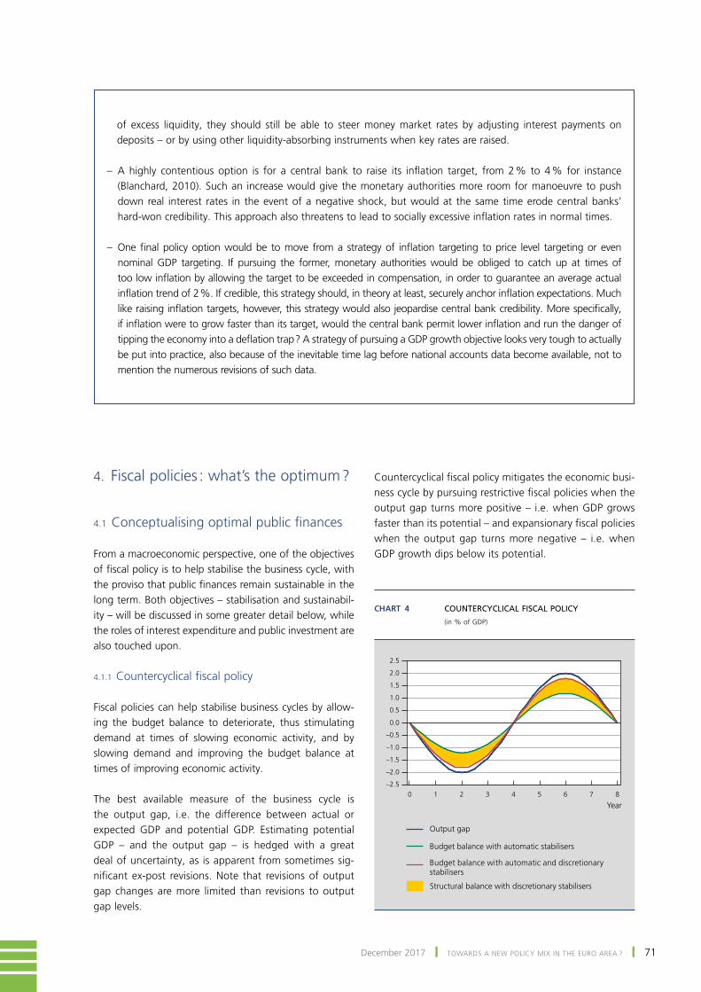
71December 2017 ❙ toWARDS A NEW polIcY mIX IN tHE EuRo AREA ? ❙
of excess liquidity, they should still be able to steer money market rates by adjusting interest payments on deposits – or by using other liquidity-absorbing instruments when key rates are raised.
– A highly contentious option is for a central bank to raise its inflation target, from 2 % to 4 % for instance (Blanchard, 2010). Such an increase would give the monetary authorities more room for manoeuvre to push down real interest rates in the event of a negative shock, but would at the same time erode central banks’ hard-won credibility. This approach also threatens to lead to socially excessive inflation rates in normal times.
– One final policy option would be to move from a strategy of inflation targeting to price level targeting or even nominal GDP targeting. If pursuing the former, monetary authorities would be obliged to catch up at times of too low inflation by allowing the target to be exceeded in compensation, in order to guarantee an average actual inflation trend of 2 %. If credible, this strategy should, in theory at least, securely anchor inflation expectations. Much like raising inflation targets, however, this strategy would also jeopardise central bank credibility. More specifically, if inflation were to grow faster than its target, would the central bank permit lower inflation and run the danger of tipping the economy into a deflation trap ? A strategy of pursuing a GDP growth objective looks very tough to actually be put into practice, also because of the inevitable time lag before national accounts data become available, not to mention the numerous revisions of such data.
4. Fiscal policies : what’s the optimum ?
4.1 Conceptualising optimal public finances
from a macroeconomic perspective, one of the objectives of fiscal policy is to help stabilise the business cycle, with the proviso that public finances remain sustainable in the long term. Both objectives – stabilisation and sustainabil‑ity – will be discussed in some greater detail below, while the roles of interest expenditure and public investment are also touched upon.
4.1.1 Countercyclical fiscal policy
Fiscal policies can help stabilise business cycles by allow‑ing the budget balance to deteriorate, thus stimulating demand at times of slowing economic activity, and by slowing demand and improving the budget balance at times of improving economic activity.
the best available measure of the business cycle is the output gap, i.e. the difference between actual or expected gDp and potential gDp. Estimating potential GDP – and the output gap – is hedged with a great deal of uncertainty, as is apparent from sometimes sig‑nificant ex-post revisions. Note that revisions of output gap changes are more limited than revisions to output gap levels.
Countercyclical fiscal policy mitigates the economic busi‑ness cycle by pursuing restrictive fiscal policies when the output gap turns more positive – i.e. when GDP grows faster than its potential – and expansionary fiscal policies when the output gap turns more negative – i.e. when GDP growth dips below its potential.
Chart 4 COUNTERCYCLICAL FISCAL POLICY
(in % of GDP)
0 1 2 3 4 5 6 7 8–2.5
–2.0
–1.5
–1.0
–0.5
0.0
0.5
1.0
1.5
2.0
2.5
Budget balance with automatic stabilisers
Budget balance with automatic and discretionary stabilisers
Output gap
Structural balance with discretionary stabilisers
Year

72 ❙ toWARDS A NEW polIcY mIX IN tHE EuRo AREA ? ❙ NBB Economic Review
Automatic stabilisers are eminently suitable instru‑ments to help stabilise business cycles, kicking into action without requiring discretionary government in‑tervention. Examples include tax revenues falling and unemployment benefit rising when economic activity slows. Automatic stabilisers may be complemented by discretionary countercyclical policies, which do require policy decisions, e.g. raising public consumption and in‑vestment or other spending, or cutting taxes when eco‑nomic demand weakens. In the European governance framework, stabilisation through automatic stabilisers has always been accepted.
A country’s fiscal multiplier captures the extent to which its fiscal policy is able to stabilise its business cycle. This multiplier will be higher at times of recession and if monetary policy is constrained in its pursuit of accom‑modating policies, as in the case of a liquidity trap, as described above. In addition, it has been demonstrated that a major negative demand shock can permanently affect economic activity, because initially cyclical unem‑ployment can turn partly structural, for example (the hysteresis effect). This can increase the need to introduce discretionary stabilising policy at times of a steep eco‑nomic slowdown.
If it is to have a lasting effect, countercyclical fis‑cal policies require symmetry, meaning that buffers must be created at times of a positive output gap to fund the fiscal stimulus when the output gap turns negative.
4.1.2 Sustainable public finances
Optimal fiscal policy also means that public finances must remain sustainable. that is to say, the government needs to remain solvent and able to meet its current debt com‑mitments. In formal terms, it must fulfil its intertemporal budget constraint, i.e. the value of government debt must equal the present value of future primary surpluses. The sustainability of public finances is determined by past financial commitments (the present debt ratio) and ex‑pected future liabilities (including the cost of population ageing) and economic growth.
Whereas stabilisation is a short‑term objective, the sus‑tainability of public finances is a longer-term concern. on average, then, the sustainability objective should be respected across a full business cycle, but cannot prevent public finances from temporarily deteriorating as the cycle worsens.
Chart 5 SUSTAINABLE PUBLIC FINANCES MEANS FURTHER FISCAL CONSOLIDATION FOR SOME COUNTRIES
(in % of GDP)
ES PT IT FR SI BE SK IE LV EE FI AT LT CY MT NL LU DE
–4
–3
–2
–1
0
1
2
–4
–3
–2
–1
0
1
2
Medium-term objective (MTO)
Structural balance in 2017
Consolidation effort still required to achieve MTO
Fiscal margin
Sources : EC, NBB.(1) For Greece, a new MTO has not yet been defined, since it is still subject to an assistance programme.

73December 2017 ❙ toWARDS A NEW polIcY mIX IN tHE EuRo AREA ? ❙
unlike stabilisation, sustainability is not a symmetrical goal. A country will do well to consolidate if it drifts too far away from its sustainability objective, but there is no such thing as consolidating too far in terms of this objective.
The need for fiscal consolidation may on occasion be con‑trary to the stabilisation objective, particularly in the event of an economic slowdown.
For fiscal purposes, the European Commission calculates a minimum medium-term objective (minimum MTO) for each individual country, which should guarantee the sus‑tainability of public finances if respected. This minimum mto is expressed in terms of a target structural balance, allowing for budgetary balance fluctuations as a result of automatic stabilisers. When calculating the minimum MTO, the Commission will factor in the required budget effort to reduce a country’s debt to 60 % of GDP if its debt ratio currently exceeds 60 %, the required budgetary bal‑ance to stabilise the debt ratio at 60 % of GDP, and a pre-financing by one-third of the expected costs of ageing by 2060. The Fiscal Compact subsequently stipulates that a euro area country’s minimum MTO should not be below a structural balance of –1 % of GDP if its debt level is below 60 % of GDP or below –0.5 % of GDP if its debt level is above 60 % of GDP. Member States may always commit to a stricter mto than the one suggested by the European commission. Belgium’s minimum mto, for instance, has been set at –0.5 % of GDP, but its federal government has posited a structural balance in its stability programme.
Sustainability conditions vary greatly for the euro area countries, with some needing to massively improve their budgetary balance, e.g. Spain, france, portugal, Italy, Slovenia and Belgium. other countries – germany, luxembourg, malta and the Netherlands – have already achieved or exceeded their mtos and are looking at a measure of fiscal margin.
4.1.3 the role of interest expenditure
What role does interest expenditure on government debt play relative to a fiscal policy’s macroeconomic objectives ? Is the optimum fiscal policy best defined in terms of the primary budgetary balance, ignoring interest expenditure developments and seeing interest expenditure changes as a bonus or a penalty ? Or should an optimum fiscal policy be defined in terms of the budgetary balance that takes interest expenditure into account ? Deciding the best course of action requires a closer look at the various pos‑sible factors informing interest expenditure developments.
Developments in interest expenditure on government debt depend on developments in implicit interest rates
Chart 6 PUBLIC INVESTMENT IS CURRENTLY VERY LOW IN SOME EUROPEAN COUNTRIES (FIXED CAPITAL INVESTMENT, 2016)
–2
–1
0
1
2
3
4
5
JJ
J
J
J J
JJ
J
J J
J
JJJ
SE FI LU DK NL FR AT UK EA BE DE IT ES IE PT
Gross fixed capital formation
p.m. 2000-2007 average
Net investment
Source : EC.
and the debt ratio. for a given debt structure, changes in implicit interest rates break down into three components. The first is a cyclical component tied in with a country’s monetary policy, reflecting inflation targets and the busi‑ness cycle, with accommodating monetary policies typi‑cally causing rates to fall. Second, a structural component reflects fundamental factors such as demographic trends and productivity growth, with lower potential growth making for lower interest rates, for example. The third component is a risk premium reflecting default risk, with a lower default risk causing rates to fall.
Different causes of falling (or rising) interest rates justify fiscal policy easing (or tightening) from a macroeconomic perspective. Accommodating monetary policy had better not be thwarted by restrictive fiscal policy, lower potential growth necessitates productive government spending, while a lower debt ratio or lower default risk creates mar‑gins that can be used. It is appropriate, then, to define op‑timum fiscal policy in terms of budgetary balance (includ‑ing interest expenditure). Under the current circumstances, this implies that interest income may be used and does not need to be saved up.
4.1.4 public investment
public investment and other public spending can strongly boost economic activity and an economy’s production

74 ❙ toWARDS A NEW polIcY mIX IN tHE EuRo AREA ? ❙ NBB Economic Review
4
Box 2 – Optimal fiscal policy rule
Based on the concept of an optimal fiscal policy from a macroeconomic perspective, we can postulate a rule for optimum fiscal policy, pulling together both stabilisation and sustainability objectives – which do not result in unanimous budget advice in all circumstances. For reasons set out above, this rule is defined in terms of the budgetary balance, which includes interest expenditure.
In terms of the sustainability objective, our rule postulates that the budgetary balance should at least be at a sustainable level (SUST) when the business cycle is neutral. This equals the outcome of the basic formula the European Commission uses to calculate a country’s minimum MTO, but without any limits and rounding subsequently applied by the Commission (1). For Belgium, this sustainability level works out at a budget deficit of 0.4 % of GDP. This level should basically be maintained across a full business cycle.
To stabilise the business cycle, the rule indicates that the budgetary balance may fluctuate around its sustainable level as a function of the output gap (OG). A negative output gap requires a lower and a positive output gap a higher balance. the degree of stabilisation is expressed by stabilisation parameter α. the value of α depends on the degree to which discretionary stabilisation is imposed in addition to automatic stabilisation, and therefore equals the sum of the automatic stabilisation parameter σ and discretionary stabilisation parameter δ. The value of σ typically varies by country, taking account of the semi-elasticity of the budget balance with respect to the output gap, as calculated by the Ec. to some extent, the choice of the level of stabilisation parameter α is arbitrary, and in the proposed rule it is put at one. the value of α is the same for all euro area countries, which implies that countries with relatively major automatic stabilisation (such as Belgium with σ at 0.61) require less discretionary stabilisation than those with less automatic stabilisation.
In sum, the optimum budgetary balance equals the total of the sustainability level plus the product of stabilisation parameter α and the output gap. the rule may be expressed in terms of nominal budgetary balance (BB) and structural balance (SB). As the structural balance neutralises the impact of the business cycle through automatic stabilisers, the stabilisation parameter for it reduces to the parameter for discretionary stabilisation (δ=α‑σ) :
BBt = SUST + α OGt opt
SBt = SUST + δ OGt opt
(1) Meaning that we only consider MTO 3 – which factors in the required fiscal effort to reduce a country’s debt to 60% of GDP, the fiscal balance needed to stabilise the debt ratio at 60% of GDP and a pre-financing of one-third of the expected costs of ageing by 2060 – and not MTO 1, which incorporates a safety margin relative to the 3% deficit limit, nor MTO 2, which imposes an absolute minimum of -0.5% and -1% of GDP respectively when the debt is lower or higher than 60% of GDP.
potential, and a country would be well advised to encour‑age such capital spending, particularly in current condi‑tions of low interest rates and low potential growth. However, in numerous euro area countries public invest‑ment is currently at low levels, for instance in Belgium and germany. And Ireland, portugal and the mediterranean countries, hit hard by the financial and economic crisis, have also made deep cuts in their public investment.
public investment in as much as it expands a country’s capital stock – i.e. if it exceeds depreciation – will contribute to higher gross government debt, but not to net government debt. more productive investment does not necessarily mean that public finances become less sustainable, and any evaluation of the sustainability objective may therefore consider the level of net public investment.

75December 2017 ❙ toWARDS A NEW polIcY mIX IN tHE EuRo AREA ? ❙
If the budgetary balance dips below the optimum balance, a sustainability problem arises. In this case the budgetary balance will need to change towards the optimum level, factoring in the change in the output gap which the optimum level is tied in with :
The speed of the return to the optimum level is an arbitrary choice. But the rule here posited proposes narrowing the differential between actual and optimum budgetary balance by one-quarter every year, or by 0.5 % of GDP if this one-quarter is below 0.5 % of GDP, until such time as the optimum level is achieved.
When the budgetary balance exceeds the optimum level, no sustainability problem exists. the proposed optimum budget rule does not prescribe a return to the optimum budgetary balance in such a case ; only changes in the business cycle need factoring in :
RULE FOR OPTIMUM FISCAL POLICY, SHOWN FOR NEGATIVE OUTPUT GAP
(in % of GDP)
0 1 2 3 4 5 6 7 8Year
No sustainability problem
Sustainability problem
positive output gap positive output gapnegative output gap
worsening reviving
Sustainable budgetary balance (SUST)
Change in structural balance for stabilisation objective
Change in structural balance for sustainability objective
–2.0
–1.5
–1.0
–0.5
0.0
0.5
Optimum structural balance (= SUST + δ OG)
ΔBBt = max[0.5;1/4 (BBt-1 – BBt-1 )] + α ΔOGtopt
ΔSBt = max[0.5;1/4 (SBt-1 – SBt-1 )] + δ ΔOGtopt
ΔBBt = α ΔOGt
ΔSBt = δ ΔOGt
4

76 ❙ toWARDS A NEW polIcY mIX IN tHE EuRo AREA ? ❙ NBB Economic Review
Countries that enjoy a fiscal margin on their sustainability objective are thus not encouraged to use it up : after all, the stabilisation objective is symmetrical, the sustainability objective is not.
The chart shows the proposed rule for an optimum fiscal policy in the event of a negative output gap and is expressed in terms of the structural balance. The structural balance’s optimum level goes down as the business cycle deteriorates and moves back up when economic activity revives. At times when the output gap is closed (in years 2 and 6 in the chart) the optimum structural balance typically equals the sustainable level (SUST), pegged at –0.5 % of gDp in the graph.
If the structural balance dips below the optimum level and the business cycle deteriorates (point bottom left), the stabilisation objective prescribes the adoption of a discretionary expansionary policy (green arrow) whereas the sustainability objective points to a discretionary restrictive policy (red arrow). Recommended policy is the sum of both and is either expansionary or restrictive depending on the extent of the consolidation problem. If the structural balance is below the optimum level and economic activity is on the up (point bottom right), both stabilisation and sustainability objectives prescribe a restrictive policy. Here too, recommended policy is the sum of both. If the structural balance is above optimum level (points above the blue line) there is no sustainability problem and only the stabilisation objective applies (see green arrows).
Finally, it is worth noting that the proposed fiscal rule is predicated on a number of key principles underpinning optimum fiscal policy, which have been translated into a simple formula. To some extent the choice of the values of the parameters and variables is arbitrary within these formulas, and might possibly be refined. Stabilisation parameter α, for one, could itself serve as a function of the output gap to allow for the increased effectiveness of stabilisation policies when economies slump. Sustainability level SUST could be adjusted in proportion to a country’s net public investment level, given its minor effect on sustainability. In terms of the business cycle measure, i.e. the output gap, the – frequently significant – ex-post revisions are a major issue. However, our rule-based fiscal recommendations primarily rely on changes in the output gap, which are less subject to revision.
4.2 Optimum fiscal policies for individual countries
4.2.1 Applying proposed rule
Determining individual countries’ optimum fiscal policy requires an adequate indicator that serves as a point of reference for the actual or expected budgetary outcomes.
Based on the proposed rule in box 2, individual euro area countries’ optimal fiscal policies are compared with actual or forecast budget outcomes, as the chart below does for the euro area’s six biggest economies. The optimum fiscal policy is expressed in terms of a change in the structural balance, with calculations based on output gap data as currently estimated – and therefore not on output gap projections at the time these budgets were drawn up. Exercise outcomes should be read on a year‑to‑year basis, and are not cumulative.
In 2007, before the onset of the crisis, Belgium, the Netherlands and France pursued expansionary fiscal
policies, whereas the proposed rule flags a need for sig‑nificant consolidation efforts to ensure the sustainability of their public finances. At the time, Germany, Italy and Spain, by contrast, did stick to fiscal policies that matched their sustainability objective.
At the time of the financial and economic crisis (2008-10) there was actually scope for discretionary expansion‑ary fiscal policies, but Belgium, France, the Netherlands and Spain allowed their budgetary balances to deterio‑rate further than the rule proposed. By contrast, Italy made only limited use of discretionary stimuli.
In the 2012-13 period, Germany, the Netherlands, Italy and Spain pursued very restrictive fiscal policies, whereas a dete‑riorating business cycle justified neutral to expansionary poli‑cies. It is worth noting here, with the benefit of hindsight, that the business cycle in Italy and Spain deteriorated much more sharply than was forecast when their budgets were drawn up. After all, if these countries had used the output gap projections at the time, the proposed rule would have advised restrictive fiscal policies for Spain and Italy.

77December 2017 ❙ toWARDS A NEW polIcY mIX IN tHE EuRo AREA ? ❙
Looking at 2017-18, Belgium, France, Italy and Spain should be pursuing much more of a consolidation effort than is expected to emerge on the basis of the European commission’s most recent outlook (2017 autumn projections), given the current uptick in the business cycle combined with a sustainability problem.
4.2.2 European budgetary framework recommendations compared with proposed rule
An interesting exercise is to compare 2017 and 2018 recommendations flowing from our proposed rule with country-specific recommendations emerging from the European budgetary framework.
In terms of their levels, recommendations for france and Belgium broadly fall in line with the proposed rule’s. However, the rule points to a more significant consolida‑tion for Spain and Italy, as the output gap in both coun‑tries is closing rapidly and they are also facing significant sustainability issues. All things considered, European
budgetary framework recommendations make a lot of sense right now and should be observed.
germany and the Netherlands have no sustainability problems and the commission has not issued any recom‑mendations for these countries. The proposed fiscal rule suggests that a slightly restrictive fiscal policy is the way to go for the Netherlands in 2017 and 2018, and for Germany in 2018, simply because their economic activity has been on the way up. After all, according to the fiscal rule, neither country is asked to use their margins towards the sustainability objective.
Although the recommendations under the Stability and Growth Pact currently make sense, there are key differences with the proposed rule for optimum fiscal policy. In terms of the optimum level of the budgetary balance, the rule also allows discretionary stabilisation on top of the automatic stabilisers ; the proposed rule is more relaxed in times of worsening business cycles and stricter when cycles are on the up. If a structural balance drops to below the optimum level, the SGP
Chart 7 OPTIMUM FISCAL POLICIES IN INDIVIDUAL COUNTRIES
(change in structural balance, in % of GDP)
XXXXXXXX
XXXX
2007
2008
2009
2010
2011
2012
2013
2014
2015
2016
2017
2018
XXX
X
XXXXXXXX
2007
2008
2009
2010
2011
2012
2013
2014
2015
2016
2017
2018
X
X
X
XX
XXXX
X
XX
2007
2008
2009
2010
2011
2012
2013
2014
2015
2016
2017
2018
XX
X
XXXXXXXX
X
2007
2008
2009
2010
2011
2012
2013
2014
2015
2016
2017
2018
2007
2008
2009
2010
2011
2012
2013
2014
2015
2016
2017
2018
X
XX
XX
XXXXXXX
2007
2008
2009
2010
2011
2012
2013
2014
2015
2016
2017
2018
–6–5–4–3–2–10123
4
X
XXXX
X
XXXXXX
BELGIUM GERMANY NETHERLANDS
FRANCE ITALY SPAIN
–3.0–2.5–2.0–1.5–1.0–0.50.00.51.01.52.0
–3.0–2.5–2.0–1.5–1.0–0.50.00.51.01.52.0
–3.0–2.5–2.0–1.5–1.0–0.50.00.51.01.52.0
–2.0–1.5–1.0–0.50.00.51.01.52.02.5
3.0
–3.0–2.5–2.0–1.5–1.0–0.50.00.51.01.52.0
Actual (or predicted)
Proposed budget rule
Sources : EC, ESCB, NBB.

78 ❙ toWARDS A NEW polIcY mIX IN tHE EuRo AREA ? ❙ NBB Economic Review
only permits no improvement in the structural bal‑ance in very exceptional circumstances, i.e. when the output gap falls below –4 % of GDP or when growth turns negative. In all other circumstances, countries are obliged to improve their structural balances or at least stay on an even keel. By contrast, the proposed rule does permit a deteriorating structural balance when business cycles turn down, even in the case of a sus‑tainability problem. that said, any improvement in the business cycle would impose a larger structural balance improvement on countries.
4.3 Optimum fiscal policy for the euro area as a whole
4.3.1 fiscal policy stance
Calculating the fiscal position of the euro area as a whole is a purely mechanical exercise, aggregating member States’ fiscal positions and not determining it directly. So, fiscal policy at euro area level is the result of discretion‑ary policies at national level. The euro area fiscal position
is shown here in the shape of the structural balance, as released by the European commission.
Fiscal policy for the euro area as a whole between 2010 and 2018 can be broken down into a number of sub-periods. In the period 2008-2010, the financial crisis and its subsequent economic recession caused steep deficits and rising debts in the wake of the countercyclical policies of the time, severely damaging the state of the euro area’s public finances. From 2011, the euro area countries started to reduce their deficits to improve the sustainability of pub‑lic finances. The procyclical fiscal approach at the time of the 2012-13 double dip was informed by an updated and tightened Stability and Growth Pact. With the benefit of hindsight, this period’s fiscal policy may be judged to have been too restrictive, with the fiscal consolidation carried out too soon, partly as a result of pressure from financial mar‑kets on some countries. The fiscal position of the euro area as a whole was largely neutral from 2014, in line with the cyclical state of affairs. Recent economic data is encourag‑ing, revealing strengthening growth and a closing output gap. This strongly improved business situation would sug‑gest a rather more restrictive fiscal policy.
Chart 8 RECOMMENDATIONS FROM EUROPEAN BUDGETARY FRAMEWORK CURRENTLY USEFUL
(change in structural balance, in % of GDP)
2017 2018 2017 2018
2017 20182017 20182017 2018
2017 2018
n. n. n. n.
BELGIUM GERMANY NETHERLANDS
SPAIN
0.0
0.2
0.4
0.6
0.8
1.0
0.0
0.2
0.4
0.6
0.8
1.0
0.0
0.2
0.4
0.6
0.8
1.0
1.2
1.4
1.6
0.0
0.2
0.4
0.6
0.8
1.0
1.2
1.4
1.6
0.0
0.2
0.4
0.6
0.8
1.0
1.2
1.4
1.6
Country-specific recommendations (EC ; Ecofin Council)
Proposed fiscal rule
0.0
0.2
0.4
0.6
0.8
1.0
FRANCE ITALY
Sources : EC, NBB.

79December 2017 ❙ toWARDS A NEW polIcY mIX IN tHE EuRo AREA ? ❙
In the past year, key international institutions made recom‑mendations on optimum fiscal policy for the euro area as a whole in 2017 and 2018 (1). For 2017, the Ecofin Council and the IMF counselled the euro area as a whole to steer a neutral policy course, taking into account cyclical con‑siderations and the sustainability of public finances in the long term. Note, however, that as late as an end-2016 publication, the European commission still espoused an ex‑pansionary fiscal policy (2) . For 2018, first-half publications by the European commission, the European fiscal council and the IMF continued to argue for a largely neutral fiscal policy. In a speech at the end of September, the director of the Imf’s European Department, poul thomsen, noted that the advice had been changed to a gradually restrictive policy : “With growth recovering quite strongly and output gaps narrowing fast, now is the time to rebuild fiscal space and place public debt on a firm downward trajectory. Gradual fiscal consolidation would help ensure that, when the next adverse shock hits, the euro zone is on a stronger footing and has the necessary buffers (3).”
Chart 9 FISCAL POLICY FOR THE EURO AREA AS A WHOLE
(in % of GDP)
X
X
X
XX X X X X
2010
2011
2012
20132014 2015 2016
–5
–4
–3
–2
–1
0
1
–4 –3 –2 –1 210
2017 r 2018 r
No sustainability problem
Sustainability problem
Output gap
Stru
ctur
al b
alan
ce
Actual (or predicted)
Optimum fiscal policy (1)
Is a more restrictive fiscal policy desirable ?
Sources : EC, NBB.(1) According to the proposed rule for optimal fiscal policy in box 2. This works out
as follows : a change in the output gap by 1 % of GDP will prompt a change in the structural balance by 0.44 % of GDP and a change in the nominal budgetary balance by 1 % of GDP through the automatic stabilisers (0.56 % of GDP) and a discretionary policy impulse (0.44 % of GDP) ; the proposed budget deficit for the medium term amounts to 0.5 % of GDP.
(1) Note that recommendations by the European Commission, the Ecofin Council and the European Fiscal Board all refer to the structural primary balance, whereas the Imf bases its recommendations on the structural budgetary balance.
(1) EC (2016b).(2) IMF (2017b).
This recap shows that the past year has seen the views of international institutions evolve on the issue of the appropriate fiscal policy, from a rather expansionary to a largely neutral fiscal policy, and more recently to a gradu‑ally restrictive one. the shift is attributable to an improved economic situation and outlook, allowing the output gap to close in 2018 and even become slightly positive. The recommendation to gradually adopt restrictive policies matches the findings set out previously.
4.3.2 Optimum fiscal policy for the euro area in current conditions
The optimum fiscal policy for the euro area as a whole does not necessarily equal the sum of optimum fiscal policies for the individual countries, for a number of rea‑sons. for one thing, only cyclical considerations come into play at the euro area level, not the sustainability of public finances, as the euro area itself does not have any public debt. Besides, the fiscal policy impact differs : fiscal mul‑tipliers, which reflect the impact of a budgetary stimulus on economic activity, are typically higher for the euro area as a whole than for individual countries, as a budgetary stimulus in the relatively more open individual economies in part “leaches away” in the shape of spillovers. This es‑sentially means that, at the level of the euro area, achiev‑ing the stabilisation objective requires a relatively smaller effort than the sum of the individual countries’ required efforts – from a stabilisation perspective, that is.
Having weighed up all these considerations, we propose calculating the optimum fiscal policy for the euro area as a whole by three pathways :
1. A GDP-weighted sum of the optimum change in the structural balance of the individual euro area coun‑tries, based on the proposed fiscal rule factoring in both stabilisation and sustainability objectives. the outcome reflects the overall state of play at euro area level if all individual countries pursued their optimum fiscal policies. For the euro area as a whole, this fis‑cal rule notes a structural balance improvement of 0.5-0.6 % of GDP.
2. A variation of the previous sum total, in which indi‑vidual countries enjoying fiscal margins – under the proposed rule and in terms of their sustainability ob‑jective – (partially) avail themselves of these margins, implying a symmetrical application of the individual countries’ sustainability objective. If countries without sustainability problems, such as germany and the Netherlands, actually used their fiscal margins, the sum for the euro area as a whole would be lower by around 0.2 percentage points of GDP.

80 ❙ toWARDS A NEW polIcY mIX IN tHE EuRo AREA ? ❙ NBB Economic Review
3. A third pathway is calculated as the GDP-weighted sum of the optimum change in the euro area coun‑tries’ structural balance, taking into account the stabi‑lisation objective only (and ignoring the sustainability objective). This throws up a slightly restrictive fiscal policy for the euro area as a whole, as explained by an improving business cycle. the recommended improve‑ment in the structural balance is slightly lower than in the second pathway.
All three sets of calculations arrive at an optimum fiscal policy which is restrictive for the euro area as a whole in both 2017 and 2018, but differ in the extent to which the structural balance should improve. this illustrates our earlier assertion of a difference between an optimum fis‑cal policy for the euro area as a whole (pathway 3 – pure stabilisation objective) and the sum of the optimum fiscal policies for the individual countries (pathway 1 – pro‑posed fiscal rule). The Five Presidents’ Report envisaged a European stabilisation mechanism to help bolster this central level to bridge these differences. this suggestion is discussed in section 6 of this article.
Finally, it is worth pointing out that our findings for the optimum fiscal policy in the euro area as a whole in 2017 and 2018 – which should be restrictive, on our
calculations – differ from policies as currently in place, which are still slightly expansionary.
5. Germany : the engine powering the euro area ?
Section 4 has shown that, if Germany used its budgetary margin, fiscal policy would be less restrictive in the euro area as a whole. There have been frequent calls for a more stimulating fiscal policy in Germany. In this context, over the past few years, Germany’s current account surplus has claimed centre stage in the debate over euro area economic policies and rebalancing. It was assumed that, by winding down its surplus by investing more, Germany would support activity in the other euro area countries, particularly those facing a demand shortfall – countries that had yet to close the output gap – that did not have any scope for more supportive fiscal policies.
Under the EU’s macroeconomic imbalance procedure (MIP), germany has been considered a member State displaying macroeconomic imbalances since 2014, in view of its signif‑icant and persistent current account surplus. In its July 2017 country-specific recommendations, the EU Council stated that germany’s persistently high current account surplus is
Chart 10 OPTIMUM FISCAL POLICY FOR THE EURO AREA
(in % of GDP)
2017 2018 2017 2018
CHANGE IN STRUCTURAL BALANCE CHANGE IN STRUCTURAL PRIMARY BALANCE
Proposed fiscal rule (1)
Proposed fiscal rule + use of fiscal margins (2)
Pure stabilisation objective (without sustainability objective)
0.0
0.1
0.2
0.3
0.4
0.5
0.6
0.7
0.0
0.1
0.2
0.3
0.4
0.5
0.6
0.7
Sources : EC, NBB.(1) Calculated as the GDP-weighted average of the euro area countries’ objectives, taking into account stabilisation and sustainability objectives.(2) As in 1 but with countries that enjoy fiscal margins – i.e. countries without sustainability issues – putting their margins (partly) towards expansionary fiscal policies
(by applying symmetrically the proposed fiscal rule on sustainability).

81December 2017 ❙ toWARDS A NEW polIcY mIX IN tHE EuRo AREA ? ❙
relevant beyond its own borders and that addressing the issue may influence the rebalancing perspectives of the rest of the euro area and the European union because more dynamic domestic demand in germany may help ease the deleveraging needs in heavily‑indebted member States.
5.1 germany’s high and persistent current account surplus reflects German economy’s savings surplus
There is no doubt : Germany has a very high current account surplus. In 2016, the surplus nudged 8.5 % of GDP, well in excess of the MIP-defined critical threshold of 6 % of GDP and the highest level currently recorded in the major advanced economies. Over the past few years, this increase has mostly been fed by a growing trade surplus (goods) – which stood at 8.7 % of GDP in 2016 – mostly with countries outside the euro area. There has been a shift in the geographic breakdown of Germany’s trade surplus from euro area countries to countries outside the euro area. Germany likewise booked a revenue surplus, and IMF (2017d) calculations put the implicit return on
Germany’s foreign assets at about 0.5 of a percentage point ahead of that on its foreign liabilities.
In addition to its competitive export‑oriented manufacturing industry, Germany’s external surplus also reflects the econo‑my’s significant domestic savings surplus. In the past couple of years, households and firms have been recording a net lending surplus, while the government’s borrowing require‑ment was cleared in the aftermath of the financial crisis.
Households’ financing surplus is the biggest component in germany’s savings surplus. It has shrunk slightly since 2010, as private consumption and spending on residential build‑ings has picked up. german households’ savings ratio is high (one of the highest among OECD countries) and reflects de‑mographic factors. concerns over the population’s ageing, which is happening more rapidly in Germany than in most other major economies, persuaded german households to save to keep their standard of living in retirement. the uptick in the savings ratio after the turn of the century coincided with a time in which major reforms of the country’s public pension system were decided and in which average pension replacement rates fell. moreover, additional private pension
Chart 11 CURRENT ACCOUNT AND LENDING BALANCES IN GERMANY
(in % of GDP)
1996
1998
2000
2002
2004
2006
2008
2010
2012
2014
2016
–10
–5
0
5
10
15
1996
1998
2000
2002
2004
2006
2008
2010
2012
2014
2016
–10
–5
0
5
10
15
Goods
Services
Revenues
Transfers
Total : current account
Government
Corporations
Households
Total relative to rest of the world
CURRENT ACCOUNT LENDING BALANCES BY SECTOR
Source : EC.

82 ❙ toWARDS A NEW polIcY mIX IN tHE EuRo AREA ? ❙ NBB Economic Review
schemes had become more attractive for tax purposes with the so‑called Riester scheme starting up in 2002.
Furthermore, non-financial corporations have been record‑ing a steep upturn in their funding surplus after 2000, which may well be down to a confluence of country-specific factors. Wage restraint and labour market reforms (Hartz) tempered wage bills, and Germany’s corporations would not appear to be committing all of these extra funds to raising their domestic capital stock but to have also put some of that money towards reducing their reliance on external funding. As a result, German corporations, which had already boasted low debt ratios compared with the rest of the euro area, have reduced their debt further still.
germany’s current account surplus in general and the sav‑ings surplus of its non-financial corporations in particular are also linked to direct foreign investment by german corporations in the shape of offshoring (parts of) their pro‑duction to Eastern Europe and other emerging countries. Adding to germany’s competitiveness, this move has pro‑ductivity‑enhancing effects, especially by substituting do‑mestic manufactured goods with cheaper intermediate im‑ports, while the threat of relocation abroad may well have reined in wage trends in export-oriented manufacturing.
germany’s integration in global value chains is increasingly considered a fundamental feature of the german economy, and the country’s stock of gross foreign direct investment (FDI) has advanced fairly rapidly. Within the euro area, a large proportion of its fDI has ended up in luxembourg and increasingly also in the Netherlands, as well as in Belgium, France, Austria, Italy and Spain, while German FDI was limited in Greece and Portugal. Outside the euro area, the United Kingdom, Switzerland and Eastern European nations such as poland, the czech Republic and Hungary are important host countries. Expressed as a percentage of the host countries’ gDp, germany’s fDI presence is strongest in most of its neighbouring countries in the euro area (Luxembourg, the Netherlands, Austria and Belgium) and in Eastern Europe (Hungary, czech Republic, Slovakia and Poland). In relation to the size of these economies, its presence is less important in france, Italy and the euro area countries hardest hit by the crisis (Spain, Portugal, Greece). the country’s strong representation in its Eastern European neighbours reflects its expansion into the global value chains in those countries.
Research has shown that FDI typically complements do‑mestic investment : FDI is reported to have positive effects on domestic investment activity. However, in the case of Germany findings are mixed and there is some evidence that german fDI serves as a substitute for domestic in‑vestment in the long term (Herzer D. and m. Schrooten,
2007). The proximity of lower-wage countries in Central and Eastern Europe is reported to have played an impor‑tant role in this.
5.2 Is investment too low in Germany ?
Aside from the export‑oriented manufacturing indus‑try, a reduced public sector borrowing requirement, high household savings ratios and corporate germany’s competitiveness, the country’s current account surplus – reflected in its economy’s savings surplus – is often also
Chart 12 INVESTMENT BY SECTOR IN GERMANY
(in % of GDP)
2002
2003
2004
2005
2006
2007
2008
2009
2010
2011
2012
2013
2014
2015
2002
2003
2004
2005
2006
2007
2008
2009
2010
2011
2012
2013
2014
2015
2002
2003
2004
2005
2006
2007
2008
2009
2010
2011
2012
2013
2014
2015
BUSINESS INVESTMENT
PUBLIC INVESTMENT
HOUSEHOLDS
10.0
10.5
11.0
11.5
12.0
12.5
13.0
13.5
0.0
0.5
1.0
1.5
2.0
2.5
3.0
3.5
4.0
4.5
3.0
4.0
5.0
6.0
7.0
8.0
9.0
Germany Euro area excluding Germany
Source : EC.

83December 2017 ❙ toWARDS A NEW polIcY mIX IN tHE EuRo AREA ? ❙
ascribed to (domestic) investment spending, which is con‑sidered to be merely moderate.
When we break down this investment spending by sector (households, corporations and government), we find that german household spending on residential property as a percentage of gDp has been higher on average than in the other euro area countries in the past few years. Granted, the german construction industry languished in the dol‑drums for years (until about 2009), having overheated after German unification, but since then investment in residential buildings has really taken off. Some sources (Dahl j. and m. Góralczyk, 2017) claim there is still a shortage of housing and housebuilding is expected to stay robust.
germany’s business investment ratio, by contrast, still lags a little behind the rest of the euro area. that said, it is worth remembering that – as noted above – FDI by german corporations may to some extent prove a substi‑tute for domestic investment in the long term. german non-financial corporations using a proportion of their re‑sources to strengthen their positions in global value chains could consequently partly explain their lacklustre domestic investment activity shown up by certain measures.
finally, germany’s public investment ratio turns out to fall short of government investment in other euro area coun‑tries. Coupled with the finding that post-crisis investment picked up rather slowly in the German sector for other build‑ings and structures (including infrastructure), this tallies with the conclusions of the in-depth review (IDR) by the European Commission in its 2017 MIP that investment in transport, en‑ergy and telecoms infrastructure has run into delays and that recent efforts to facilitate and encourage public investment have so far had limited effects. In addition, the perceived quality of German railways, waterways and aviation infra‑structure would also seem to have suffered.
Some sources suggest that germany’s subdued public investment is due not so much to a lack of political will or funding, but that other detracting factors come into play, such as capacity shortages and the complexity of proce‑dures, rules governing major infrastructure works and financial relations in the public sector (1). Country-specific
conditions also hamper international comparisons. german authorities have argued that german public investment is underestimated, as the statistical perim‑eter for germany’s public sector is different from that in other countries. factoring in investment projects currently funded by the government as well as public procurement and measures taken to address capacity issues, public investment may be expected to rise in the years ahead.
All told, a range of fundamental factors may have con‑spired to create germany’s considerable balance of pay‑ments surplus, but international institutions such as the Imf and the European commission reckon that these factors are not enough to fully explain the current account surplus – a not insignificant proportion remains unexplained. This unexplained component is likely due to other country‑specific factors, such as Germany’s integration in global value chains, which encourages the competitiveness of the german economy (2), but is hard to capture in the usual economic models. Research suggests that germany using its available fiscal policy margin would only have a modest impact in getting its current account surplus down (3).
5.3 Who benefits from budgetary stimulus in Germany ?
In the debate about a possible role for greater german investment dynamics in economically reviving and rebal‑ancing the euro area, the question arises as to what the extent and geographical breakdown would be of such a policy’s impact on the other euro area countries.
Recent years have seen a growing interest in the spillover effects of budgetary policies, after the crisis, its subsequent recovery programmes and budgetary consolidation had demonstrated their importance. However, the outcomes of economic research into this phenomenon vary greatly (4), depending on the type of transmission mechanism studied (trade, financial markets, confidence effects), the character‑istics of the countries facing budgetary shocks, the monetary policy response (and its effects on the exchange rate), the fis‑cal policy breakdown (higher multiplier deriving from public investment than from tax cuts), possible changes in multipli‑ers across the cycle (higher for strongly negative output gap), separate or coordinated shock, how the shock is funded, budgetary stimulus coupled with austerity in the medium term, fixed or floating exchange rates – the list goes on.
for the euro area, too, research has produced a variety of outcomes. the importance of the monetary policy re‑sponse is often highlighted : the effects recorded under unchanged monetary policy that has reached the zero lower bound (ZLB) for key policy rates drop off sharply (or
(1) Council of the European Union (2017),“Council Recommendation of 11 July 2017 on the 2017 National Reform programme of germany and delivering a Council opinion on the 2017 Stability Programme of Germany” (2017/C 261/05), Official Journal of the European Union, C261/18, 9/8/2017, consideration 8; IMF (2017d), “Germany 2017 Article IV consultation – Staff report”, IMF Country Report 17/192, July 2017; Deutsche Bank (2017), Focus Germany, 6 April.
(2) ECB (2017), “The impact of global value chain participation on current account imbalances,” Economic Bulletin Issue 2, p.68 and p.81.
(3) See IMF (2017d), “Germany 2017 Article IV consultation – Staff report”, IMF Country Report 17/192, July, Box 1.; Kollmann R., M. Ratto, W. Roeger, J. in ‘t Veld and L. Vogel. (2014), “What drives the German current account? And how does it affect other EU member states?”, European Economy, Economic papers 516, April, p. 25.
(4) For a literature review, see Attinasi M-G., M. Lalik and I.Vetlov (2017), Fiscal spillovers in the euro area, a model-based analysis, EcB Working paper Series 2040, march.

84 ❙ toWARDS A NEW polIcY mIX IN tHE EuRo AREA ? ❙ NBB Economic Review
even turn negative) if monetary policy responds to higher growth and inflation.
A number of studies have pointed up the unequal distri‑bution of spillover effects across the different euro area countries, with the differences typically explained by the intensity of trade links. Researchers often conclude that the bulk of the effect of additional public investment in germany may be expected to be felt in its neighbouring countries – and particularly the small and medium‑sized ones – while its impact should be muted on countries further afield and not directly on Germany’s borders (1).
By extension, important information can be gleaned from an overview of added value derived from trading partners and incorporated in german investment, shedding light on the potential geographical distribution of direct trading effects of an expansion in investment spending in germany. Data are available in the oEcD’s trade in value‑added indicators. the value added content generated by the respective trading partners is expressed in proportion to their total value added.
As the chart reveals, the direct trading effects of invest‑ment in germany on its European trading partners’ economic activity would indeed be highest for a num‑ber of small to medium‑sized countries in the proxim‑ity of germany, both inside and outside the euro area, specifically the Czech Republic, Austria, Luxembourg, Switzerland and Hungary. Broadly speaking, value added
creation in German investment would appear relatively important to those countries with which Germany has forged global value chains. the impact looks smaller on euro area countries whose economic activity might ben‑efit most from additional support.
All-in all, a German budgetary expansion would not cur‑rently appear appropriate in terms of the business cycle. In fact, an expansionary fiscal policy would contribute relatively little to a reduction in the country’s current ac‑count surplus. Even so, focused public investment in in‑frastructure might still be favourable for potential growth in germany.
6. Does the European policy framework require adjusting ?
6.1 A more active role for fiscal policy in the policy mix
The foundations of the European budgetary framework were laid with the Maastricht Treaty and the Stability and Growth Pact (SGP), which implements the require‑ments of the treaty regarding budgetary surveillance. the budgetary framework supports and coordinates Member States’ fiscal policies. As noted in section 1 of this article, the framework chiefly focuses on the sustainability of public finances and assigns only a limited role to fiscal pol‑icy in stabilising the business cycle through the operation of automatic stabilisers. The framework breaks down into a preventive arm, which aims to prevent unsustainable budgetary situations, and a corrective arm, which imposes corrective measures for Member States struggling with major problems in their public finances (2).
The current set-up begs the question of how fiscal policy could play a more active role in the policy mix, in particular at times of deep recession and monetary policy limita‑tions. A number of adjustments have already been made, while others have been proposed.
A first such adjustment to have euro area countries’ fiscal policies take greater account of cyclical factors came at the beginning of 2015, when a new matrix was launched to determine required structural balance improvements in the Sgp’s preventive arm. When identifying improvement
(1) See Deutsche Bundesbank (2016), The international spillover effects of an expansion of public investment in germany, Monthly Report, August ; Cwik, T. and V. Wieland (2010), Keynesian government spending multipliers and spillovers in the euro area, ECB Working Paper 1267, November ; Beetsma R., M. Giuliodori and F. Klaassen (2005), Trade spillovers of fiscal policy in the European Union : a panel analysis, DNB Working paper 52, August.
(2) For an extensive overview of the European budgetary framework, see Melyn W., L. Van Meensel and S. Van Parys (2015).
Chart 13 VALUE ADDED CONTENT OF GERMANY’S GROSS FIXED CAPITAL FORMATION (1) ORIGINATING FROM EUROPEAN TRADING PARTNERS
(by country of origin, all sectors, in % of total value added of country of origin, averages for 2007-2011)
CZ AT LU CH
HU
BG LV SK PL RO SI EE HR SE LT BE
DK FI PT ES IT EL FR NL
CY IE UK IS
NO
0.0
0.5
1.0
1.5
2.0
2.5
3.0
Source : OECD.(1) No distinction in gross fixed capital formation by government and private sector.

85December 2017 ❙ toWARDS A NEW polIcY mIX IN tHE EuRo AREA ? ❙
requirements, the new matrix now does (more) factor in economic conditions, with a greater effort imposed in favourable business cycles than when economic times are bad. Another adjustment already in place was the creation of the European fiscal Board and its role. Set up in October 2015, the Board is to ensure improved compli‑ance with fiscal rules and a more robust coordination of national fiscal policies. In this latter capacity, the European Fiscal Board has been tasked with assessing the appropri‑ate fiscal policy course, at both national level and in the euro area. In October 2016, the European Commission appointed its chair and four members, and the council released its first report on 20 June 2017, which chiefly consisted of an assessment of appropriate future fiscal policy for the euro area.
one further adjustment of Sgp rules might be to change the approach to public investment and encourage a more favourable treatment of such expenditure. the current framework already has some clauses stimulating public investment, but any Sgp reforms should be the right time to urge a change to considering depreciation on investment instead of gross investment expenditure when determining the budgetary balance in the preven‑tive arm. Such a shift would imply that the government’s overall balance is adjusted for net investment, and in this way, an investment boost would not be hindered (1). In the current environment, this would appear an obvi‑ous way to stimulate public investment – low in quite a few countries. The basic rules of the European budget‑ary framework, such as the deficit limit of 3 % of GDP and the debt rule included in the corrective arm of the SGP, would not be changed, however. In this way, the budgetary responsibility and the sustainability of public finances in the long term would still be guaranteed. It would also seem advisable to seriously consider the crea‑tion of a European stabilisation mechanism, in keeping with the proposals in the Five Presidents’ Report.
6.2 Is there a need for a European stabilisation mechanism ?
In view of past shocks, it appears essential that the euro area would now have access to adequately robust instru‑ments to absorb such shocks and enhance its resilience without endangering the sustainability of public finances.
Even already resilient economies boasting sufficiently flexible labour markets and healthy public finances have no guarantees that all risks could be eliminated and that all shocks could be smoothly reduced. Some economic shocks may simply cut too deep to be handled solely on the interface of national automatic stabilisers and a cen‑tralised monetary policy.
A European stabilisation mechanism (2) might be con‑sidered to complement the stabilising role of national budgets and monetary policy, especially insofar as the Stability and Growth Pact is focused on the objective of sustainability, as markets may sometimes behave ir‑rationally and given the dilemma of implementing at a national level an adequate fiscal policy set up for the broader euro area. Such a mechanism might be defined as a policy aiming at smoothing national economic cycles by means of “automatic” and “certain” – that is, known beforehand – transfers between Member States, which would also improve the countercyclical fiscal stance of the euro area.
Quite a bit of thinking has already gone into the crea‑tion of such a mechanism, envisaging common insurance mechanisms, or even resources funded by member States’ contributions. Such funds would factor in where countries are in their economic cycles and would be set up in such a way that transfers are automatically activated at times of recession. A vital precondition for any such mechanism would be that it does not fuel moral hazard or create permanent transfers, does not throw up any obstacles to necessary adjustments and does not prevent structural measures meant to address the deeper causes of the mac‑roeconomic imbalances that still exist in some countries.
overall, three options come on the fore (3) :
i) A European Investment Protection Scheme could kick in during an economic downturn – as evidenced by a negative output gap – by providing support for specific investment priorities already planned up front, such as infrastructure development, invest‑ment in education and skills, or in specific types of public investment (frequently the first item in na‑tional budgets to be cut).
ii) A European Unemployment Reinsurance Scheme, which, unlike funds using the output gap as refer‑ence variable, would be based on unemployment levels (immediately observable). Given widely dif‑ferent national labour market institutions and initial unemployment levels, these mechanisms would have to complement national unemployment benefits.
(1) Melyn W., R. Schoonackers, P. Stinglhamber and L. Van Meensel (2016). (2) more generally, such mechanism of solidarity should necessarily go hand in hand
with the reduction of risks, more particularly an established fiscal discipline and a convergence of national policies towards the best practices. Moreover, there are other channels, but these are either not yet fully developed – e.g. the capital markets union – or likely to be largely affected by crises, as evidenced by bank lending drying up in some countries and the fragmentation that has hindered monetary policy transmission in the past.
(3) See EC (2017a), amongst others.

86 ❙ toWARDS A NEW polIcY mIX IN tHE EuRo AREA ? ❙ NBB Economic Review
iii) A “rainy day fund” could collect regular contributions, with disbursements made on a discretionary basis in the event of shocks. Such payments would neverthe‑less stay limited to the accumulated contributions. the fund’s capacity might therefore be too small in case of a major shock.
conclusions
A key lesson from the financial and economic crisis is that the various policy instruments – and particularly monetary and fiscal policies – should be complementary to achieve the desired results. An active fiscal policy, for one, might prove useful in the event of a very deep recession or when monetary policy runs into limitations.
These observations have led us to investigate what would be an optimum fiscal policy. Clearly, fiscal policies pursued in some euro area countries and in the euro area as a whole in the 2012-13 crisis were too restrictive.
In the period after that and to date, the euro area as a whole has been on a more neutral policy course, which has proven appropriate. It would appear, though, that most euro area countries should pursue rather more re‑strictive fiscal policies in 2018, as economic activity gains momentum, output gaps are closing and the sustainabil‑ity of public finances needs to be guaranteed.
Germany enjoys some fiscal margin, but a budgetary ex‑pansion would not currently appear desirable for business cycle reasons and its impact on euro area countries where economic activity would benefit the most from additional support would be small anyway. By contrast, focused public investment in infrastructure, would be a sensible way to bolster growth potential.
lastly, a European stabilisation mechanism should be considered under certain circumstances to make sure that optimum fiscal policy in the euro area as a whole, where only the stabilisation function comes into play, matches optimum policies in the individual countries.

87December 2017 ❙ toWARDS A NEW polIcY mIX IN tHE EuRo AREA ? ❙
Bibliography
Ademmer E., C. Boeing-Reicher, J. Boysen-Hogrefe, K.-J. Gern, U. Stolzenburg (2016), Euro-area fiscal stance : definition, implementation and democratic legitimacy, provided at the request of the Economic and Monetary Affairs Committee of the European parliament, july.
Akerlof G. and R. Shiller (2009), Animal Spirits. How Human Psychology Drives the Economy, and Why It Matters For Global Capitalism, princeton university press, princeton.
Attinasi M-G., M. Lalik and I. Vetlov (2017), Fiscal spillovers in the euro area, a model-based analysis, EcB, Working paper Series 2040, march.
Aucremanne L. and S. Ide (2010), “Lessons from the crisis : monetary policy and financial stability”, NBB, Economic Review, September, 7‑20.
Auerbach A. and M. Obsfeld (2003), The case for open-market purchases in a liquidity trap, NBER, Working Paper 9814, July.
Auerbach A., Y. Gorodnichenko (2012), “Fiscal multipliers in recession and expansion”, in Alesina A. and F. Giavazzi (eds.), Fiscal policy after the financial crisis, Chicago, University of Chicago Press, 63-98.
Banco de España (2017), “Spillover effects of national fiscal policy in the euro area”, Box 4.1 in Annual Report 2016.
Bankowski K. and M. Ferdinandusse (2017), Euro area fiscal stance, EcB, occasional paper 182, january.
Beetsma R., M. Giuliodori and F. Klaassen (2005), Trade spillovers of fiscal policy in the European Union : a panel analysis, DNB Working paper 52, August.
Belke A. and T. Osowski (2016), Measuring fiscal spillovers in EMU and beyond : A Global VAR approach, cEpS Working Document 428, December.
Bénassy-Quéré A. and Cimadomo J. (2006), Changing patterns of domestic and cross-border fiscal policy multipliers in Europe and the US, cEpII Working papers, 2006‑24, December.
Bénassy-Quéré A. (2016), Euro-area fiscal stance : definition, implementation and democratic legitimacy, provided at the request of the Economic and Monetary Affairs Committee of the European Parliament, July.
Bénassy-Quéré A., X. Ragot and G. Wolff (2016), Which fiscal union for the euro area ?, Bruegel policy Contribution 2016 / 05, February.
Bernanke, B., M. Gertler and S. Gilchrist (1996), “The Financial Accelerator and the Flight to Quality”, Review of Economics and Statistics, Symposium on Developments in Business Cycles Research, 78 :1, February, 1-15.
Bernanke, B. (2004), The Great Moderation, Remarks at the meetings of the Eastern Economic Association, Washington, DC, 20 February.
Blanchard O. and J. Gali (2007), “Real Rigidities and the New Keynesian Model”, Journal of Money, Credit and Banking, Proceedings of the Conference on Quantitative Evidence on Price Determination, February, 35-66.
Blanchard O., G. Dell’Ariccia and P. Mauro (2010), “Rethinking macroeconomic policy”, Journal of Money, Credit and Banking, 42, 199‑215.
Blanchard O., C.J. Erceg and J. Lindé (2015), Jump starting the euro area recovery : would a rise in core fiscal spending help the periphery ?, NBER, Working paper 21426, july.

88 ❙ toWARDS A NEW polIcY mIX IN tHE EuRo AREA ? ❙ NBB Economic Review
BNP Paribas (2017), “Allemagne, les infrastructures menacées”, Eco Week, 24 February.
Boeckx J., N. Cordemans and M. Dossche (2013), “Causes and implications of the low level of the risk-free interest rate”, NBB, Economic Review, September, 63-88.
Boeckx J. and M. Deroose (2016), Monetary and fiscal policy in the euro area : independent but connected, NBB, Economic Review, September, 7‑26.
Boeckx, J. and N. Cordemans (2017), “Monetary Policy in the wake of the Great Recession”, Reflets et perspectives de la vie économique, 56, De Boeck Supérieur.
Botev J., J. Fournier and A. Mourougane (2016), A Re-assessment of Fiscal Space in OECD Countries, oEcD, Economics Department Working Paper 1352, November.
Buti, M. (2016), “What future for rules-based fiscal policy ?”, in Progress and Confusion – The State of Macroeconomic Policy, ed. Blanchard O., R. Raghuram, K. Rogoff, and L.H. Summers, MIT Press, Cambridge, Massachusetts, 183-195.
Capital Economics (2017), “German investment set for strong growth”, European Economics Update, 20 September.
Council of the European Union (2017), “Council Recommendation of 11 July 2017 on the 2017 National Reform programme of germany and delivering a council opinion on the 2017 Stability programme of germany”, Official Journal of the European Union, 9 August.
Cordemans N., M. Deroose, M. Kasongo Kashama and A. Stevens (2016), “The ABC of quantitative easing or the basics of central bank asset purchases”, NBB, Economic Review, june, 29‑41.
Cwik T. and V. Wieland (2010), Keynesian government spending multipliers and spillovers in the Euro area, EcB, Working paper Series 1267, November.
Dahl J. and M. Góralczyk (2017), “Recent supply and demand developments in the German housing market”, European Economy Economic Brief 025, may.
De Jong J., M. Ferdinandusse, J. Funda, I. Vetlov (2017), The effect of public investment in Europe : a model-based as-sessment, EcB, Working paper Series 2021, february.
De Backer B., J. Wauters (2017), “The cyclical and structural determinants of the low interest rate environment”, NBB, Economic Review, September.
De Grauwe P. (2013), Design Failures in the Eurozone : Can they be fixed ?, lEQS paper 57, february.
Deutsche Bank (2017), Focus Germany, 6 April.
Deutsche Bundesbank (2011), “Germany’s external position against the background of increasing economic policy sur‑veillance”, Monthly Report, october.
Deutsche Bundesbank (2016), “The international spillover effects of an expansion of public investment in Germany”, Monthly Report, August.
Draghi M. (2014), Unemployment in the Euro Area, Address at the federal Reserve Bank of kansas city jackson Hole Symposium, 22 August.
Dullien, S. (2012), A European unemployment insurance as a stabilization device – Selected issues, paper prepared for Eu‑level economic stabilisers seminar, European commission, Directorate‑general Employment, Social Affairs & Inclusion.

89December 2017 ❙ toWARDS A NEW polIcY mIX IN tHE EuRo AREA ? ❙
EC (2014a), “Cross-border spillovers in the euro area”, Quarterly Report on the Euro Area, 13(4), 7-22.
EC (2014b), Macroeconomic imbalances Germany 2014, European Economy – occasional papers 174, march.
EC (2015), Report on Public Finances in EMU 2015, Institutional paper 14, December.
EC (2016a), The 2016 Stability and Convergence Programmes, An Overview and Implications for the Euro Area Fiscal Stance, Institutional Paper 34, September.
EC (2016b), Towards a positive fiscal stance for the euro area, communication from the commission to the European Parliament, the Council, the European Economic and Social Committee and the Committee of the Regions, 16 November.
EC (2016c), “The policy mix, when monetary policy is constrained at the zero lower bound”, Quarterly Report on the Euro Area, 15(3), 19-28.
EC (2016d), Report on Public Finances in EMU 2016, Institutional paper 45, December.
EC (2016e), Specifications on the implementation of the Stability and Growth Pact and guidelines on the format and content of Stability and Convergence Programmes, 5 July.
EC (2017a), Reflection paper on the deepening of the Economic and Monetary Union, COM(2017) 291, 31 May.
EC (2017b), Vade Mecum on the Stability and Growth Pact, 2017 Edition, Institutional Paper 052, March.
EC (2017c), The euro area fiscal stance and the policy mix : challenges and trade-offs, presentation at EIU, 2 March.
EC (2017d), An Overview of the 2017 Stability and Convergence Programmes and an Assessment of the Euro Area Fiscal Stance for 2018, Institutional paper 059, july.
EC (2017e), Country Report Germany 2017 including an In-Depth Review on the prevention and correction of macro-economic imbalances, staff working document, 22 February.
ECB (2012), “The role of fiscal multipliers in the current consolidation debate”, Monthly Bulletin, December, 82‑85.
ECB (2016a), “Public investment in Europe”, Economic Bulletin, Issue 2, 75‑88.
ECB (2016b), “The euro area fiscal stance”, Economic Bulletin, Issue 4, 68‑87.
ECB (2017), “The impact of global value chain participation on current account balances”, Economic Bulletin, Issue 2, 68‑82.
Eggertsson G. and M. Woodford. (2004), Optimal Monetary and Fiscal Policy in a Liquidity Trap, NBER, Working paper 10840.
EU (2017), « Council Recommendation of 21 March 2017 on the economic policy of the euro area », Official Journal of the European Union, 24 March.
European Fiscal Board (2017), Assessment of the prospective fiscal stance appropriate for the euro area, 20 June.
European Parliament (2017), The euro area fiscal stance, briefing, 23 January.
European Council (2017), Council recommendation on the economic policy of the euro area, 21 March.

90 ❙ toWARDS A NEW polIcY mIX IN tHE EuRo AREA ? ❙ NBB Economic Review
Eyraud L., V. Gaspar and T. Poghosyan (2017), Fiscal Politics in the Euro Area, Imf Working paper 17 / 18, january.
Fatas A. and L.H. Summers (2016), The permanent effects of fiscal consolidations, NBER, Working Paper 22374.
Feldstein M. (2016), “The future of fiscal policy, in progress and confusion”, in The State of Macroeconomic Policy, ed. o. Blanchard, Rajan R., Rogoff k., and Summers l.H., mIt press, cambridge, massachusetts, pp. 177‑181.
Fisher, I. (1933), “The Debt-Deflation Theory of Great Depressions”, Econometrica, 4, 337-357.
Giavazzi F. (2016), Euro-area fiscal stance : definition, implementation and democratic legitimacy, Provided at the request of the Economic and monetary Affairs committee of the European parliament, September.
Hebous S. and T. Zimmerman (2013), “Estimating the effects of coordinated fiscal actions in the euro area”, European Economic Review, 58, 110‑121.
Herzer D. and M. Schrooten (2007), “Outward FDI and domestic investment in two industrialized countries”, Economics Letters, 99, 139-143.
IMF (2013), “Multi-country report, German-Central European supply chain-cluster report”, IMF Country Report 13 / 263, August.
IMF (2015), Monetary Policy and financial stability financial Stability, Staff policy Report, August.
IMF (2016), Euro Area Policies, Staff Report for the 2016 Article IV Consultation with Member Countries, july.
IMF (2017a), Euro Area Policies, Staff Report for the 2017 Article IV Consultation with Member Countries, july.
IMF (2017b), The Euro Zone : What’s Next, speech by Poul Thomsen, Director of the European Department, 28 September.
IMF (2017c), 2017 External Sector Report, policy paper, july.
IMF (2017d), “Germany 2017 Article IV Consultation—Staff Report”, IMF Country Report 17 / 192, july.
IMF (2017e), “Germany, Selected issues”, IMF Country Report 17 / 193, July.
IMF (2017f), World Economic Outlook, october.
In ‘t Veld J. (2013), Fiscal consolidations and spillovers in the Euro area periphery and core, European Economy – Economic papers 506, october.
In ‘t Veld J. (2016), “Public Investment Stimulus in Surplus Countries and their Euro Area Spillovers”, European Commission Economic Brief 016, August.
Juncker, J.-C. (2017), Speech on the state of the Union 2017, given to the European parliament, Strasbourg, 13 September.
Keynes J.-M. (1936), The General Theory of Employment, Interest and Money, macmillan, london.
Kolerus C., I Koske and F. Hüfner (2012), Selected aspects of household savings in Germany, evidence from micro-data, oEcD Economics Department Working papers 999, November.
Kollmann R., M. Ratto, W. Roeger, J. in ‘t Veld and L. Vogel (2014), What drives the German current account ? And how does it affect other EU member states ?, European Economy – Economic papers 516, April.

91December 2017 ❙ toWARDS A NEW polIcY mIX IN tHE EuRo AREA ? ❙
Melyn W., L. Van Meensel and S. Van Parys (2015), “European governance framework for public finances : presentation and evaluation”, NBB, Economic Review, September, 73-99.
Melyn W., R. Schoonackers, P. Stinglhamber, L. Van Meensel (2016), “Should government investment be promoted ?” NBB, Economic Review, September, 99-113.
Melyn W., L. Van Meensel, S. Van Parys (2016), “The sustainability of public finances in the context of population age‑ing”, NBB, Economic Review, December, 87-103.
Mourre G., C. Astarita, S. Prince (2014), Adjusting the budget balance for the business cycle : the EU methodology, European Commission, Economic Papers 536, November.
National Institute of Economic Research (NIER) (2008), The NIER’s Conceptual Framework for Fiscal Policy, occasional Studies 16, march.
OECD (2016), “Making public finances more growth and equity-friendly”, OECD Economic Surveys : Euro Area, june.
OECD (2017a), Economic Outlook, may.
OECD (2017b), Germany – Economic forecast summary, june.
Orphanides, A. (2017), The Fiscal-Monetary Policy Mix in the Euro Area : Challenges at the Zero Lower Bound, European commission, Discussion paper 060, july.
Poghosyan T. (2017), Cross-country spillovers of fiscal consolidations in the Euro area, Imf Working paper 17‑140.
Taylor J. (1993), “Discretion Versus Policy Rules in Practice”, Carnegie-Rochester Conference Series on Public Policy , 39, 195 –214.
Turrini, A. (2008), Fiscal policy and the cycle in the Euro Area : The role of government revenue and expenditure, European Commission, Economic Papers 323, May.
Viñals, J. (2016), “Monetary policy in the future – Introduction to the monetary policy section”, in Progress and Confusion : The State of Macroeconomic Policy, ed. Blanchard o., R. Rajan, k. Rogoff, and l.H. Summers, mIt press, cambridge, massachusetts, 121‑127.

93December 2017 ❙ UP OR OUT ? PORTRAIT OF YOUNG HIGH-GROWTH FIRMS IN BELGIUM ❙
Up or out ? Portrait of young high-growth firms in Belgium
J. De MulderH. GodefroidC. Swartenbroekx (*)
Introduction
In a context of limited growth potential, it is important to understand the factors that encourage or encumber the rapid expansion of young enterprises, and in particular those that facilitate the emergence of what is referred to in the literature as “gazelles”, or young firms that post high growth rates during their first years of existence. these gazelles are in fact often frontrunners in using new technologies and / or putting new business models in place and their performance makes a significant contribu‑tion to job creation. Helping young businesses to flourish can also have positive spillover effects for the Belgian economy as a whole. This article analyses the charac‑teristics of young firms’ development in Belgium (up to their fifth year of activity). To this end, different sources of microeconomic data are used.
The article is divided into four main parts. The first one reviews some of the literature devoted to growth of young businesses and compares the situation in Belgium with that in other European countries on the basis of the figures available. The second part gives a definition of a young high-growth firm for the purposes of this article and sets out the method used. the third part maps young businesses that record rapid growth, inter alia by looking at their geographic location and by breaking them down by branch of activity. the fourth part outlines several no‑table features of these enterprises, especially as regards
their national and international trade relations, as well as their structure in terms of employment. the article is wrapped up with the main conclusions and a series of policy recommendations.
1. Literature review
1.1 Small and young high-growth enterprises
According to Gibrat (1931), the (employment) growth of a firm is a random, unpredictable phenomenon, and therefore not related to its initial size (or its age). If this is the case, it makes little sense to attempt to determine the characteristics of high-growth firms. Nevertheless, several later research papers suggest that this “Gibrat’s law” does not apply to small and / or young enterprises.
The first empirical analyses carried out by Birch (1979 and 1981) pointed up the more than proportional role that small firms play in job creation in the United States (in other words, it is not the large well-established firms that are the main source of new jobs). Since then, analyses concentrating on the growth dynamics of firms have been widened to other countries and characteristics. For instance, Haltiwanger et al. (2013) underlined that it is young firms in particular that contribute a great deal to net job creation : the inverse relationship between size and net employment growth is attributable to the fact that these young firms generally tend to be small. When
(*) The authors would like to thank E. Dhyne for his expertise in the use and analysis of microeconomic databases.
94 ❙ UP OR OUT ? PORTRAIT OF YOUNG HIGH-GROWTH FIRMS IN BELGIUM ❙ NBB Economic Review
they survive, their growth rates exceed those of well-established firms. Their probability of exit is also higher, just as the resultant job destruction rate is proportionally higher and effectively means that these young businesses have to grow in order to survive (up or out).
International analyses carried out by various authors show that the demographic features of high-growth firms are related to their age, their size, or even the branch in which they operate. Despite the wide range of definitions of a high-growth firm, research work aimed at characterising them converges on four points : they refer to a small num‑ber of firms ; they were at the origin of most job creation in developed countries ; they tend to be young and are not over‑represented in the technology branches, as might have been expected, but can actually be found across all branches of the economy (Coad and Moreno, 2015). In fact, whatever definition is selected to describe the sub-population of high-growth firms, it tends to be the knowledge-intensive firms that are over-represented in it in comparison to those with high technology content, suggesting in itself that it is mainly the level of human capital that matters in the emergence of these enterprises (Daunfeldt, Elert and Johansson, 2015). Analyses covering several different periods have also pointed up the dif‑ficulty for these firms to keep up this high rate of growth in the long run (Daunfeldt and Halvarsson, 2014). All this makes the introduction of targeted economic support policies rather delicate, given the difficulty of identifying ex ante a high-growth enterprise, the phenomenon itself being highly uncertain by its very nature (Hölzl, 2016).
1.2 Situation in Belgium
There is no one definition of a young high-growth firm or gazelle. At international level, however, wide use is made of the definition established by Eurostat and the OECD (OECD, 2007), referring to an enterprise up to five years old with ten or more employees at the beginning of the observation period and posting an average annualised growth in terms of employment or turnover greater than 20 % per annum over a period of three years. Additionally and based on the same criteria, a young moderate‑growth firm is an enterprise which has an average annu‑alised growth rate of between 10 and 20 %.
It is worth noting that employment and turnover do not necessarily move in the same proportions and simply may reflect different growth profiles, as the increase in business activity can be accompanied by productivity gains. for example, a rise in sales may precede a more or less proportional recovery in employment, or a firm with rapidly expanding turnover can adopt innovations
(whether they are technical, managerial or organisational) that reduce the job content of the expansion of its activity (Davidsson et al., 2005).
In 2014, high-growth firms (measured on the basis of employment and with no age limit) in Belgium ac‑counted for 8 % of all companies employing more than ten employees (compared with 9.2 % for the EU as a whole) and 0.4 % of the total population of firms (Mignon, 2017). Just under one-third of these firms are young businesses. So, high growth is not solely the pre‑serve of young firms.
Besides, high growth does not always reflect internal growth, but may also result from merger or acquisi‑tion operations. A study by the federal planning Bureau (Dumont et al., 2017) revealed that, during the period running from 2002 to 2014, on average 4.7 % of all high-growth firms in Belgium had been involved in a merger or acquisition in the three years preceding the observation year. And among these, 0.23 % concerned young high-growth firms as targets and 0.25 % as young ‘‘acquir‑ing” firms. Young high-growth firms’ expansion through acquisition therefore concerns only a very low percentage of the population of young enterprises.
1.3 International prospects
the in‑depth comparative study of entrepreneurial dy‑namics in different countries that the oEcD has carried out (criscuolo et al., 2014) confirms that it is not so much small enterprises as young firms (less than five years old) that are more than proportionally involved in the dynam‑ics of employment growth. In this respect, young firms make their contribution, on the one hand, by creating jobs when they enter the market and by destroying jobs in the event of failure (extensive margin), and, on the other hand, through the process of job creation / destruction in companies in the normal course of business (intensive margin). The net sum of these flows is positive for compa‑nies less than five years old. The OECD analysis (Criscuolo et al., 2014 and Calvino et al., 2015), covering a sample of 18 countries, suggest that young firms are net job crea‑tors (they take up on average 17 % of jobs but account for 41 % of all jobs created). During the economic and financial crisis, new enterprises were more badly hit than well established companies. Between 2002 and 2011, their share in total employment fell back from 1.8 to 1.2 %. This vulnerability is important, given that young enterprises are behind net job creation, just as they sup‑port productivity growth and are involved in the diffusion of innovation throughout the economic fabric (Dumont and Kegels, 2016).
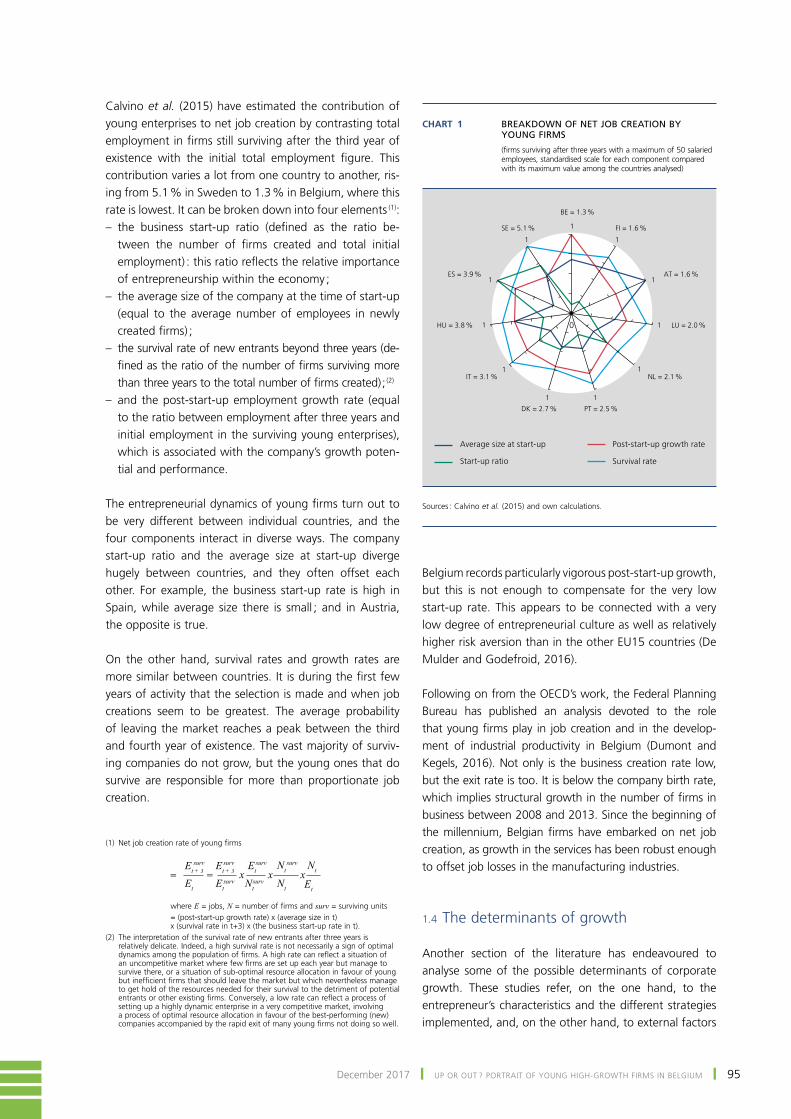
95December 2017 ❙ UP OR OUT ? PORTRAIT OF YOUNG HIGH-GROWTH FIRMS IN BELGIUM ❙
calvino et al. (2015) have estimated the contribution of young enterprises to net job creation by contrasting total employment in firms still surviving after the third year of existence with the initial total employment figure. This contribution varies a lot from one country to another, ris‑ing from 5.1 % in Sweden to 1.3 % in Belgium, where this rate is lowest. It can be broken down into four elements (1):– the business start-up ratio (defined as the ratio be‑
tween the number of firms created and total initial employment) : this ratio reflects the relative importance of entrepreneurship within the economy ;
– the average size of the company at the time of start‑up (equal to the average number of employees in newly created firms) ;
– the survival rate of new entrants beyond three years (de‑fined as the ratio of the number of firms surviving more than three years to the total number of firms created) ; (2)
– and the post-start-up employment growth rate (equal to the ratio between employment after three years and initial employment in the surviving young enterprises), which is associated with the company’s growth poten‑tial and performance.
The entrepreneurial dynamics of young firms turn out to be very different between individual countries, and the four components interact in diverse ways. The company start‑up ratio and the average size at start‑up diverge hugely between countries, and they often offset each other. for example, the business start‑up rate is high in Spain, while average size there is small ; and in Austria, the opposite is true.
On the other hand, survival rates and growth rates are more similar between countries. It is during the first few years of activity that the selection is made and when job creations seem to be greatest. the average probability of leaving the market reaches a peak between the third and fourth year of existence. the vast majority of surviv‑ing companies do not grow, but the young ones that do survive are responsible for more than proportionate job creation.
Belgium records particularly vigorous post-start-up growth, but this is not enough to compensate for the very low start-up rate. This appears to be connected with a very low degree of entrepreneurial culture as well as relatively higher risk aversion than in the other EU15 countries (De Mulder and Godefroid, 2016).
Following on from the OECD’s work, the Federal Planning Bureau has published an analysis devoted to the role that young firms play in job creation and in the develop‑ment of industrial productivity in Belgium (Dumont and Kegels, 2016). Not only is the business creation rate low, but the exit rate is too. It is below the company birth rate, which implies structural growth in the number of firms in business between 2008 and 2013. Since the beginning of the millennium, Belgian firms have embarked on net job creation, as growth in the services has been robust enough to offset job losses in the manufacturing industries.
1.4 The determinants of growth
Another section of the literature has endeavoured to analyse some of the possible determinants of corporate growth. These studies refer, on the one hand, to the entrepreneur’s characteristics and the different strategies implemented, and, on the other hand, to external factors
(1) Net job creation rate of young firms
where E = jobs, N = number of firms and surv = surviving units = (post-start-up growth rate) x (average size in t)
x (survival rate in t+3) x (the business start-up rate in t).(2) The interpretation of the survival rate of new entrants after three years is
relatively delicate. Indeed, a high survival rate is not necessarily a sign of optimal dynamics among the population of firms. A high rate can reflect a situation of an uncompetitive market where few firms are set up each year but manage to survive there, or a situation of sub‑optimal resource allocation in favour of young but inefficient firms that should leave the market but which nevertheless manage to get hold of the resources needed for their survival to the detriment of potential entrants or other existing firms. Conversely, a low rate can reflect a process of setting up a highly dynamic enterprise in a very competitive market, involving a process of optimal resource allocation in favour of the best-performing (new) companies accompanied by the rapid exit of many young firms not doing so well.
EtEt Et
surv
surv Nt Nt
Nt Nt
surv
surv surv surv
= x x xEt + 3 Et + 3 Et=
Chart 1 BREAKDOWN OF NET JOB CREATION BY YOUNG FIRMS
(firms surviving after three years with a maximum of 50 salaried employees, standardised scale for each component compared with its maximum value among the countries analysed)
1
1
1
1
1
11
1
1
1
1
0
Average size at start-up Post-start-up growth rate
Start-up ratio Survival rate
Country = net job creation in % of total employment
BE = 1.3 %
FI = 1.6 %
AT = 1.6 %
LU = 2.0 %
NL = 2.1 %
PT = 2.5 %DK = 2.7 %
IT = 3.1 %
HU = 3.8 %
ES = 3.9 %
SE = 5.1 %
Sources : Calvino et al. (2015) and own calculations.

96 ❙ UP OR OUT ? PORTRAIT OF YOUNG HIGH-GROWTH FIRMS IN BELGIUM ❙ NBB Economic Review
such as the business environment and the regulatory framework.
As for the entrepreneur’s abilities, a majority of studies have stressed the positive influence of motivation, level of education, managerial experience and the number of founders. By contrast, setting up a company after a period of unemployment tends to have a negative impact on growth. By contrast, other factors, like the gender, age or ethnic origin of the entrepreneur, do not seem to have any significant effect on the company’s performance. The adoption of a proactive, innovative and not risk averse entrepreneurial orientation is also favourable to growth (Storey, 1994. In : Davidsson et al., 2005).
The (high) growth that some companies enjoy may also be positively influenced by many different factors. As far as innovation is concerned, companies that in‑novate register a growth rate (in terms of employment and sales) double that of firms which do not innovate (Nesta, 2009). But this does not mean that there are more high-growth firms in innovating branches. An innovation strategy is not enough in itself : it has to translate into new products, while, in the case of process innovation, the impact on employment has not been determined (OECD, 2010). However, most analyses point to a positive relationship between product innovation, sales and rise in employment in high-growth enterprises (Coad and Moreno, 2015).
Adoption of an export strategy is relevant for a firm lo‑cated in a small country because it boosts the size of its market and its growth prospects. The impact on growth nevertheless depends on resources that can be mobilised to get established on an international scale, which can prove to be rather difficult for young firms in view of their (small) size and limited resources (they are less diversified). Combined with the strong(er) competition faced on the international plane, this encourages a strategy of dif‑ferentiation, which in turn leads them to focus on goods and services that meet the specific expectations of clients (Davidsson et al., 2005).
conclusion of partnership agreements and, more glob‑ally, involvement in networking, whether just within the branch itself or with clients, suppliers, distributors (in the case of international expansion) or research centres, may reinforce the resilience of high-growth enterprises (OECD, 2010).
Access to funding is also often cited as being a brake on the creation and development of a new activity / business. Young firms are frequently confronted with problems of moral hazard and adverse selection owing to the
asymmetry of information about them on the capital markets (no credit history) and the lack of collateral for securing loans (calvino et al., 2016).
While the rise of young businesses is partly dependent on the founders’ entrepreneurial capacity, the busi‑ness environment in which they are expanding and any potential obstacles that they will have to face also influence their growth dynamics. In this regard, differ‑ences between entrepreneurial dynamics also have to be set against domestic policies that apply to young firms and the regulatory framework governing them. this applies, for instance, to conditions for access to the market for goods and services, financing or withdrawal from the market (related to bankruptcy laws). Calvino et al. (2016) make a distinction between the effect of these domestic policies on new businesses and the im‑pact they have on established companies. for example, very young firms (with less than two years of activity under their belt) are systematically influenced more by the domestic economic context and by the regulatory framework than mature firms are. In fact, as they are smaller, they are less able than large firms to influence their environment.
2. Young high-growth firms in Belgium
2.1 Definition
the next part of the article highlights the results of the analysis of Belgian business data that we carried out. The findings concerning the number of young high-growth firms as well as their specific features are of course largely dependent on the definition used. If it is too wide, the number of companies qualifying would be too high and it would be pointless to try and highlight certain distinctive features. Conversely, too strict a defi‑nition would only take into account an extremely small number of enterprises, whose characteristics may not be truly representative.
In this regard, Eurostat and the oEcD’s approach to the subject (see above) has been chosen as the starting point. this approach nevertheless has some shortcom‑ings when used for the purposes of our analysis. Firms that start out small (with less than ten workers) can thus never be labelled as young high-growth firms. This point is a major limitation, especially for Belgium, which is a nation of SMEs. The authors therefore felt it would be useful to adapt and supplement this definition (see Annex 1 for a more detailed discussion of the methodol‑ogy used).

97December 2017 ❙ UP OR OUT ? PORTRAIT OF YOUNG HIGH-GROWTH FIRMS IN BELGIUM ❙
In this article, firms are considered to be gazelles, that is, they are regarded as young high-growth firms :
– on the basis of employment :• if they employ at least ten workers at the beginning of
the observation period and register annualised growth of employment greater than 20 % over a period of three years during their first five years in business ;
• or if they employ less than ten workers at the begin‑ning of the observation period and raise their staff numbers by at least seven employees over a period of three years during their first five years in business ;
or
– on the basis of turnover :• if they post a turnover of at least a € 2 million at the be‑
ginning of the observation period and record annualised growth of turnover greater than 20 % over a period of three years during their first five years in business ;
• or if they post a turnover of less than € 2 million at the beginning of the observation period and record an increase in their turnover of at least a € 1.4 million over a period of three years during their first five years in business.
This definition makes it possible to identify companies with different growth profiles (increase in turnover, rise in employment, or both of them going up at the same time) with a view to measuring any high growth. It relies on the same criteria for increase in employment as that for turno‑ver. These criteria are consistent with each other both in the case of firms that have only just reached the thresholds used (ten workers or a € 2 million turnover) and those that fall under them : the required expansion of seven members of staff or a turnover of € 1.4 million over a period of three years actually corresponds to the absolute increase implic‑itly required of companies attaining the fixed threshold.
to be able to assess the results and characteristics of young high-growth firms, these are first of all compared with the findings for young firms whose growth is said to be moderate. this corresponds to an annual increase of 10 to 20 % (or its equivalent) in employment or turnover, by using the same methodology. In addition, a second reference group is composed of all other young enter‑prises. These two control groups thus cover firms that are the same age as gazelles but which have posted lower growth. A third and final reference group includes mature firms, i.e. those that are at least ten years older than the young firms in question, covering all growth profiles.
The database covers all Belgian firms that filed their an‑nual accounts with the National Bank of Belgium over the
period running from 1996 to 2014. As the observation period spans the first five years of their existence, these companies were set up between 1995 and 2009. The annual accounts data have been combined with informa‑tion on these firms’ international trade flows found in the foreign trade statistics.
the analysis only concerns so‑called “autonomous” enterprises, and not those belonging to a multinational or a Belgian group, as their performance is more likely to be due to the possibility of transferring sales and / or employment between companies in the same group than to their own intrinsic characteristics. Moreover, it is concentrated on private sector firms. For this reason, non‑market services have been left out of the database. In view of their specific nature, agriculture, production and distribution of electricity, gas and water, as well as financial activities have not been taken into considera‑tion either.
2.2 findings
Almost 180 000 of the 215 000 autonomous companies established between 1995 and 2009 were still in activity five years later (i.e. roughly 83 %). Among these were a total of 6 133 gazelles, that is, 3.4 % of firms still in business. In addition, 6 % of this population posted moderate growth. So, average annual growth was less than 10 % for 91 % of young firms that had survived after five years.
Analysis of the date on an annual basis reveals that just over 14 000 autonomous companies on average have been formed each year over the period under review. While the trend had originally been upward – approximately 11 600 companies were founded in 1995, compared with 17 800 in 2007 –, the economic crisis subsequently brought the numbers down. On an annual basis, among the firms that were set up between 1995 and 2009 (and that were still trading after five years), on average 400 per year registered high growth rates.
Roughly half of the 6 133 gazelles have reached the required development stage in terms of workforce. In this respect, it turns out that young high-growth enter‑prises thus also create a lot of jobs. And 82 % of them have qualified just by increasing their turnover (1). this higher proportion depends on several different factors, such as the achievement of productivity gains. the fact that employment can only be gradually adjusted, unlike
(1) If the sum of the two proportions comes to more than 100 %, it is because some of the companies have registered the required growth rates in terms of both employment and turnover.

98 ❙ UP OR OUT ? PORTRAIT OF YOUNG HIGH-GROWTH FIRMS IN BELGIUM ❙ NBB Economic Review
turnover, has a role to play here too : in effect, the work‑force is often only expanded when sufficient business activity has been generated to enable them to take on one extra worker.
Roughly 29 % of the gazelles identified had initially ex‑ceeded the thresholds (or one of the thresholds). No less than 83 % of high-growth enterprises were selected on the basis of criteria applied below the thresholds (1). As expected, these results highlight the huge importance of small enterprises in the Belgian economy, and therefore the value of widening the criteria with a view to measur‑ing the high growth of young firms, which has made it possible to obtain a much more representative panel of gazelles.
3. mapping the gazelles
In order to draw a map of high-growth firms, some of their features have been analysed and compared with those of two other types of young firms and mature firms. The results obtained are merely descriptive. As no
adjustment has been made for other factors having an influence, it cannot be assumed that the bilateral consist‑ency obtained points up any direct link between the vari‑ables in question and the rapid growth of a company, so it is not possible to conclude that there is any causality.
3.1 Where are they based ?
first of all, the geographical location of the gazelles has been established. The regional breakdown revealed that, over the whole period analysed, 61 % of them had their head office in Flanders, compared with 24 % in Wallonia and 15 % in Brussels.
To move on to a more accurate analysis, the data were examined at local municipality level, with the objective of determining whether there were more gazelles in given economic zones (clusters). Logically, a (high-growth) firm has more chances of being set up in a big‑ger municipality. for the purposes of adjustments seek‑ing to take this factor into account, the total number of high-growth firms per municipality was compared with the working-age population (18-64 years). In the first place, the findings indicate that it is in Flanders and Brussels (and around them) that the most high-growth firms are created. The Antwerp (with its port) and
Chart 2 YOUNG FIRMS IN BELGIUM: BUSINESS CREATIONS, SURVIVAL AFTER FIVE YEARS AND GROWTH PROFILE
(autonomous firms set up between 1995 and 2009)
1995 1996 1997 1998 1999 2000 2001 2002 2003 2004 2005 2006 2007 2008 2009
0
2 500
5 000
7 500
10 000
12 500
15 000
17 500
20 000
Gazelles
Young moderate-growth firms
Number of business creations
Other young firms
Source : NBB.
(1) Once again, overlaps are possible, for example when firms that did not reach the thresholds at the beginning of the first sub-period of three years exceed these lower limits (or one of them) the following year – that is, at the beginning of the second sub‑period.
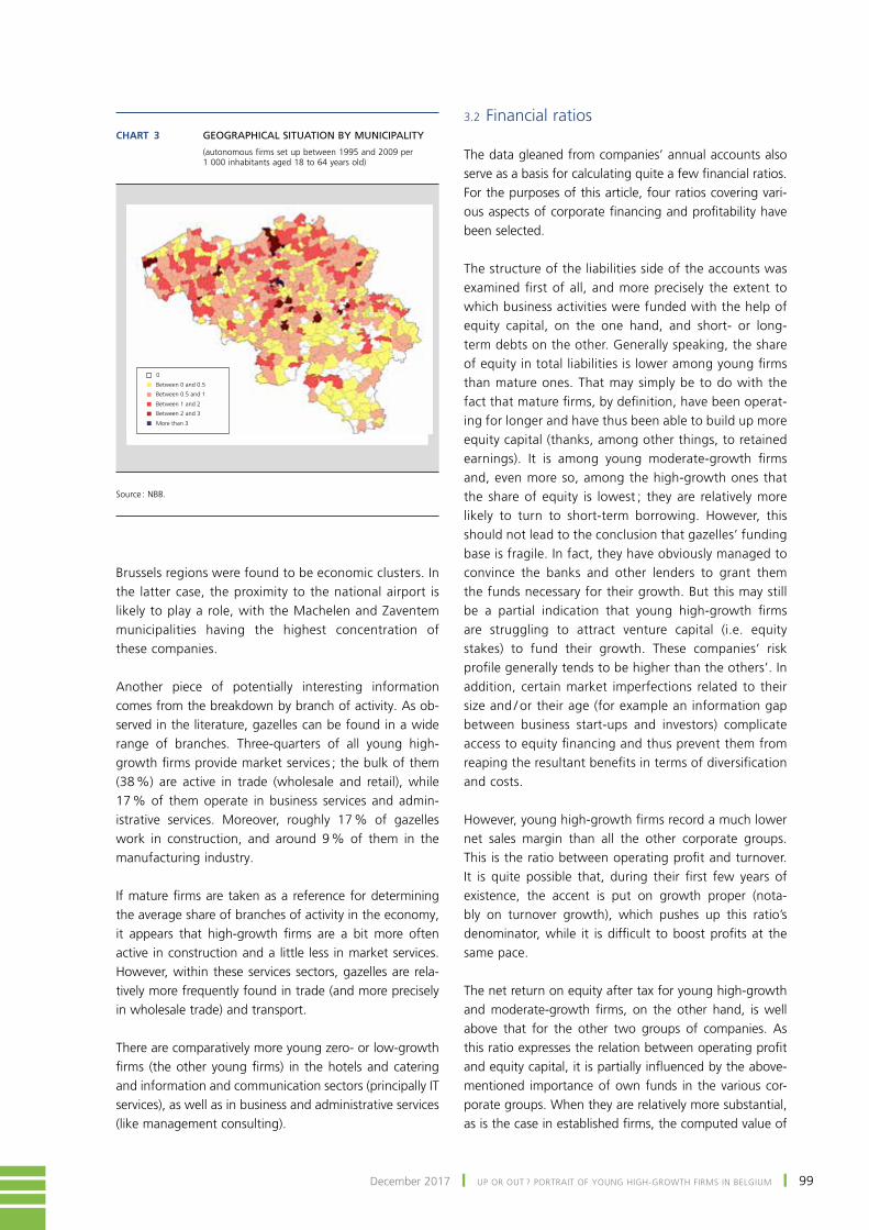
99December 2017 ❙ UP OR OUT ? PORTRAIT OF YOUNG HIGH-GROWTH FIRMS IN BELGIUM ❙
Brussels regions were found to be economic clusters. In the latter case, the proximity to the national airport is likely to play a role, with the Machelen and Zaventem municipalities having the highest concentration of these companies.
Another piece of potentially interesting information comes from the breakdown by branch of activity. As ob‑served in the literature, gazelles can be found in a wide range of branches. Three-quarters of all young high-growth firms provide market services ; the bulk of them (38 %) are active in trade (wholesale and retail), while 17 % of them operate in business services and admin‑istrative services. Moreover, roughly 17 % of gazelles work in construction, and around 9 % of them in the manufacturing industry.
If mature firms are taken as a reference for determining the average share of branches of activity in the economy, it appears that high-growth firms are a bit more often active in construction and a little less in market services. However, within these services sectors, gazelles are rela‑tively more frequently found in trade (and more precisely in wholesale trade) and transport.
There are comparatively more young zero- or low-growth firms (the other young firms) in the hotels and catering and information and communication sectors (principally It services), as well as in business and administrative services (like management consulting).
3.2 financial ratios
the data gleaned from companies’ annual accounts also serve as a basis for calculating quite a few financial ratios. for the purposes of this article, four ratios covering vari‑ous aspects of corporate financing and profitability have been selected.
The structure of the liabilities side of the accounts was examined first of all, and more precisely the extent to which business activities were funded with the help of equity capital, on the one hand, and short- or long-term debts on the other. generally speaking, the share of equity in total liabilities is lower among young firms than mature ones. That may simply be to do with the fact that mature firms, by definition, have been operat‑ing for longer and have thus been able to build up more equity capital (thanks, among other things, to retained earnings). It is among young moderate-growth firms and, even more so, among the high-growth ones that the share of equity is lowest ; they are relatively more likely to turn to short-term borrowing. However, this should not lead to the conclusion that gazelles’ funding base is fragile. In fact, they have obviously managed to convince the banks and other lenders to grant them the funds necessary for their growth. But this may still be a partial indication that young high-growth firms are struggling to attract venture capital (i.e. equity stakes) to fund their growth. These companies’ risk profile generally tends to be higher than the others’. In addition, certain market imperfections related to their size and / or their age (for example an information gap between business start-ups and investors) complicate access to equity financing and thus prevent them from reaping the resultant benefits in terms of diversification and costs.
However, young high-growth firms record a much lower net sales margin than all the other corporate groups. This is the ratio between operating profit and turnover. It is quite possible that, during their first few years of existence, the accent is put on growth proper (nota‑bly on turnover growth), which pushes up this ratio’s denominator, while it is difficult to boost profits at the same pace.
The net return on equity after tax for young high-growth and moderate-growth firms, on the other hand, is well above that for the other two groups of companies. As this ratio expresses the relation between operating profit and equity capital, it is partially influenced by the above-mentioned importance of own funds in the various cor‑porate groups. When they are relatively more substantial, as is the case in established firms, the computed value of
Chart 3 GEOGRAPHICAL SITUATION BY MUNICIPALITY
(autonomous firms set up between 1995 and 2009 per 1 000 inhabitants aged 18 to 64 years old)
0
Between 0 and 0.5
Between 0.5 and 1
Between 1 and 2
Between 2 and 3
More than 3
Source : NBB.

100 ❙ UP OR OUT ? PORTRAIT OF YOUNG HIGH-GROWTH FIRMS IN BELGIUM ❙ NBB Economic Review
the ratio falls ; and when own funds are limited, as they are for gazelles, the ratio goes up.
Lastly, liquidity in the strict sense, which relates short-term liquid assets (1) to debts payable within one year, is slightly higher in mature firms than in young firms. It is mainly in young high-growth and moderate-growth firms that this ratio is lower, because, as they tend to resort more to short-term debts to finance their business activity.
3.3 Situation after ten years
Although this article is focused on the development of companies over their first five years of activity, it is also interesting to see how they fare after that. There is always a possibility that some companies’ growth is so fast at the outset that it subsequently tapers off to virtually nothing, for instance, or even enters negative territory, or that some of them do not record any solid growth for several years. to check this, the behaviour of different groups of companies, broken down according to their growth rate over the first five years, have been examined over the next five years. To avoid any recession-related bias to the con‑clusions, only results up to the year 2007 have been taken into account. So this analysis only concerns companies set up between 1995 and 1997.
the survival rate after ten years gives an initial indication. That of firms posting high or moderate growth during the first five years (respectively between 74 and 79 %) is a lot higher than that of other young firms (66 %).
Furthermore, it is also possible to establish the growth profile of firms that have survived by applying exactly the same method as that used to break down the sample of
Chart 4 COMPOSITION OF LIABILITIES
(in % of the total, autonomous firms set up between 1995 and 2009, during their fifth year of activity)
1000 10 20 30 40 50 60 70 80 90
Mature firms
Others
Moderate-growth
Gazelles
Equity Short-term debt Long-term debt
Youngfirms
Source : NBB.
(1) This refers to liquid assets, cash investments and receivables within one year.
Chart 5 GROWTH PROFILE OF YOUNG FIRMS AFTER FIVE AND TEN YEARS
(in % of the total, autonomous firms set up between 1995 and 1997 (1))
0
10
20
30
40
50
60
70
80
90
100
Gazelles Young moderate-growthfirms
Other youngfirms
Gazelles
Young moderate-growth firms
Other young firms
Status after 5 years
Status after 10 years
Source : NBB.(1) The sample used has been scaled down to avoid any bias in the results from
the 2008 recession.

101December 2017 ❙ UP OR OUT ? PORTRAIT OF YOUNG HIGH-GROWTH FIRMS IN BELGIUM ❙
companies during their first five years of existence (1). of course, gazelles cannot be expected to continue to regis‑ter robust growth rates indefinitely : the higher the initial rate, the bigger the increase required in absolute terms to obtain the same growth rate. Thus, quite independently of their performance in the first five years, the majority of young firms are classed in the ‘other firms’ group – those whose annual average growth is less than 10 % – over the following five years. Likewise, among young firms that were also considered to be gazelles after five years, their expansion tapers off considerably : just over half of them no longer achieve the 10 % and roughly one-quarter still enjoy moderate growth. However, around 20 % of them manage to leap up to their initial growth rate of more than 20 %. They are thus clearly ahead of those firms that recorded moderate growth during their first five years of existence and are even well ahead of other young firms. In this last group, around 94 % continue to register a growth rate under 10 % ; a low initial growth rate therefore only very rarely turns into high growth. By contrast, among the firms whose growth rates were only moderate during the first five years, some 10 % moved up into the group of high-growth firms. Obviously, some businesses are not able to generate growth before several years of activity.
4. levers for development
As mentioned before, there is no one single model lead‑ing to high growth. Whether it is measured by increase in turnover or rise in employment, it actually depends on a multitude of idiosyncratic factors. moreover, it is not easy to establish a causality link between high growth and one or several firm-specific characteristics. For instance, invest‑ment projects carried out can generate a big rise in turnover making it possible to finance other investment projects.
Nevertheless, there are some common features of devel‑opment among gazelles that can be emphasised. under certain conditions, these factors are likely to make a posi‑tive contribution to their expansion over the first few years of activity and therefore turn into growth levers. With this in mind, four of them have been assessed, namely integra‑tion into the domestic production network, international expansion, level of human capital and investment. All these elements are set out in the following sections.
As the objective is to provide structural information on young high-growth firms in Belgium, the results concern enterprises set up between 1995 and 2009. On a random
basis, absence of some data has obliged us to reduce the analysis time frame.
We have chosen to examine our findings on the basis of the median rather than the average so as to prevent them from being influenced by outliers. For all the factors under consideration, statistical tests were carried out to compare the median figures for all the various sub-populations sur‑veyed (see Annex 2). All these tests produce the conclu‑sion that the median gazelle is significantly different from the median low- or negative-growth firm (other young firms), and is so right from the outset. This is also the case in comparison to the median young moderate-growth firm, except, for certain particular years of activity, when it comes to the number of suppliers, professional clients as well as amounts invested in intangible assets. Unless otherwise mentioned, the medians referred to in the rest of the article are statistically different from standard sig‑nificance thresholds.
4.1 Integration into the domestic production network
One first characteristic able to influence companies’ performance (see Dhyne and Duprez, 2015 and 2017) is their integration into the domestic production network. There are two indicators for measuring this. The first is the median number of professional clients. this shoots up considerably in the first few years of activity for young high-growth and moderate-growth firms. More precisely, in the case of these two groups of companies, the median number of professional clients more than doubles between the first and the fifth year of existence. Conversely, for young firms posting a low or negative growth rate, the median number of professional clients does not rise and actually remains below that for other groups over the entire period. It seems quite logical that a firm which grows strongly enjoys an increase in its client numbers. But it does tell us something about the mode of growth in these businesses. A firm can in fact inflate its turnover by stepping up sales to its existing clients or by enlarging its customer portfolio. It appears that investing in building up its customer portfolio is an essential stage in any company’s first few years of exist‑ence. This observation was also made by Foster et al. (2014) for the United States.
the second indicator for integration into the domestic production network is the median number of suppliers. this gives information about the degree of sophistication of the products developed in the companies. A greater number of suppliers may actually be a sign of wider di‑versification of inputs needed for production, frequently
(1) Thus, growth in employment and turnover growth are again taken into consideration for the two sub-periods of three years.
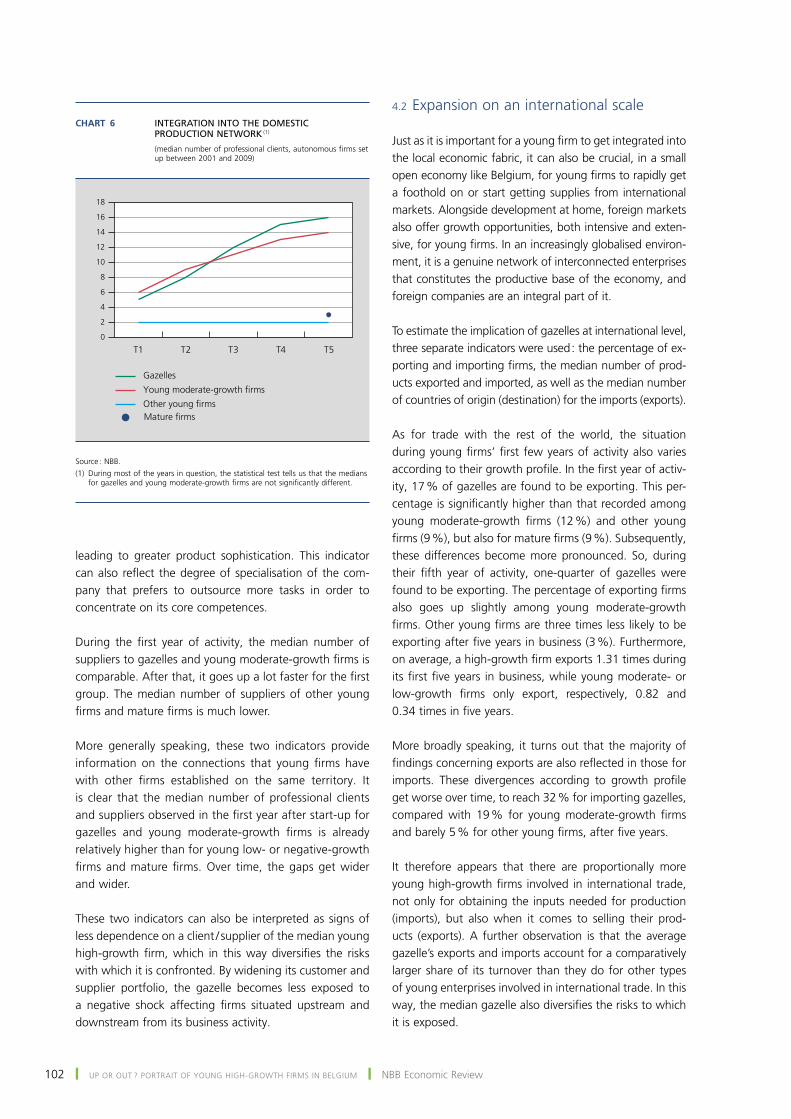
102 ❙ UP OR OUT ? PORTRAIT OF YOUNG HIGH-GROWTH FIRMS IN BELGIUM ❙ NBB Economic Review
leading to greater product sophistication. this indicator can also reflect the degree of specialisation of the com‑pany that prefers to outsource more tasks in order to concentrate on its core competences.
During the first year of activity, the median number of suppliers to gazelles and young moderate-growth firms is comparable. After that, it goes up a lot faster for the first group. the median number of suppliers of other young firms and mature firms is much lower.
More generally speaking, these two indicators provide information on the connections that young firms have with other firms established on the same territory. It is clear that the median number of professional clients and suppliers observed in the first year after start-up for gazelles and young moderate-growth firms is already relatively higher than for young low- or negative-growth firms and mature firms. Over time, the gaps get wider and wider.
These two indicators can also be interpreted as signs of less dependence on a client / supplier of the median young high-growth firm, which in this way diversifies the risks with which it is confronted. By widening its customer and supplier portfolio, the gazelle becomes less exposed to a negative shock affecting firms situated upstream and downstream from its business activity.
4.2 Expansion on an international scale
Just as it is important for a young firm to get integrated into the local economic fabric, it can also be crucial, in a small open economy like Belgium, for young firms to rapidly get a foothold on or start getting supplies from international markets. Alongside development at home, foreign markets also offer growth opportunities, both intensive and exten‑sive, for young firms. In an increasingly globalised environ‑ment, it is a genuine network of interconnected enterprises that constitutes the productive base of the economy, and foreign companies are an integral part of it.
to estimate the implication of gazelles at international level, three separate indicators were used : the percentage of ex‑porting and importing firms, the median number of prod‑ucts exported and imported, as well as the median number of countries of origin (destination) for the imports (exports).
As for trade with the rest of the world, the situation during young firms’ first few years of activity also varies according to their growth profile. In the first year of activ‑ity, 17 % of gazelles are found to be exporting. This per‑centage is significantly higher than that recorded among young moderate-growth firms (12 %) and other young firms (9 %), but also for mature firms (9 %). Subsequently, these differences become more pronounced. So, during their fifth year of activity, one-quarter of gazelles were found to be exporting. The percentage of exporting firms also goes up slightly among young moderate-growth firms. Other young firms are three times less likely to be exporting after five years in business (3 %). Furthermore, on average, a high-growth firm exports 1.31 times during its first five years in business, while young moderate- or low-growth firms only export, respectively, 0.82 and 0.34 times in five years.
more broadly speaking, it turns out that the majority of findings concerning exports are also reflected in those for imports. These divergences according to growth profile get worse over time, to reach 32 % for importing gazelles, compared with 19 % for young moderate-growth firms and barely 5 % for other young firms, after five years.
It therefore appears that there are proportionally more young high-growth firms involved in international trade, not only for obtaining the inputs needed for production (imports), but also when it comes to selling their prod‑ucts (exports). A further observation is that the average gazelle’s exports and imports account for a comparatively larger share of its turnover than they do for other types of young enterprises involved in international trade. In this way, the median gazelle also diversifies the risks to which it is exposed.
Chart 6 INTEGRATION INTO THE DOMESTIC PRODUCTION NETWORK (1)
(median number of professional clients, autonomous firms set up between 2001 and 2009)
T1 T2 T3 T4 T50
2
4
6
8
10
12
14
16
18
Young moderate-growth firms
Other young firms
Gazelles
Mature firms
Source : NBB.(1) During most of the years in question, the statistical test tells us that the medians
for gazelles and young moderate-growth firms are not significantly different.

103December 2017 ❙ UP OR OUT ? PORTRAIT OF YOUNG HIGH-GROWTH FIRMS IN BELGIUM ❙
one further point can be added to the mix to help char‑acterise the deeper integration of gazelles in international trade. the analysis of the median number of products exported after five years shows that exporting gazelles export more products (4) than young moderate- (3) or low-growth (2) exporting firms. The results for the median exporting gazelle after five years are higher than those for the median exporting mature firm.
On the import side of the equation, there seems to be even greater product diversification, in particular for importing gazelles, in the case of which the median number of products imported is 7. this median is higher than those recorded for mature importing firms (5) and for young moderate- (5) or low-to-negative-growth (2) importing firms.
It seems that the greater specialisation of the median gazelle has not just to do with a high number of do‑mestic suppliers, but it is also due to a larger number of imported products when the firm decides to source its supplies from global markets. When gazelles develop their international operations, their sales abroad also start to diversify more.
Likewise, the median number of countries of origin of imports or destination of exports varies according to
the growth profile of young enterprises. Thus, when it exports, the median gazelle sends its goods to a larger number of countries (3). This indicator is yet another example of the relatively more diversified nature of trade between gazelles and the rest of the world. This also goes for imports.
4.3 Structure of the workforce
A third source of growth for a company can also stem from the actual structure of its staff. As mentioned earlier, high-growth firms are very often active in knowledge-intensive branches. Therefore, a company’s staff skills structure should have some influence on its performance (1). Since the analysis of this dimension relied on gathering data available in the social balance sheets, and in view of the limited amount of informa‑tion, we were obliged to restrict the analysis to the period 2007-2009.
According to our data, one-fifth of all gazelles em‑ploy highly‑skilled staff (2) right from the start of their
Chart 7 INTEGRATION INTO INTERNATIONAL TRADE
(autonomous firms set up between 1995 and 2009)
T1 T2 T3 T4 T50
5
10
15
20
25
30
0
1
2
3
4
5
Young moderate-growth firms
Other young firms
Gazelles
Mature firms
Gazelles Moderate growth Others Mature firms
Number of destination countries
Number of products
EXPORTING COMPANIES(in % of the total, by category)
MEDIAN NUMBER OF EXPORTED PRODUCTS AND OF EXPORTSDESTINATION COUNTRIES
(1)
Young firms
Source : NBB.(1) After five years for young firms and after at least 15 years for mature firms.
(1) Other characteristics of the workforce were also analysed (gender, type of contract, etc.), but no significant difference between the median firms from our various groups of companies could be found for these other dimensions.
(2) to be considered as highly‑skilled, an employee must have a higher education diploma.

104 ❙ UP OR OUT ? PORTRAIT OF YOUNG HIGH-GROWTH FIRMS IN BELGIUM ❙ NBB Economic Review
business activities. this share is higher than in young moderate-growth firms (13 %) and low- or negative-growth firms (4 %). As they expand, this percentage will go up for gazelles and young moderate-growth firms. After five years in business, 37 % of gazelles em‑ploy highly-skilled staff, compared with 23 % of young moderate-growth firms and barely 5 % of low- or negative-growth firms. One-tenth of mature firms take on this type of staff.
4.4 Investment
Along with having a sufficiently skilled workforce, it is also important for young firms to invest with a view to expanding their production capacity and their innovative nature. They will thus be able to rapidly reach the tech‑nological efficiency frontier and not fall back in this area vis‑à‑vis their competitors. that could actually penalise them and jeopardise their short‑term survival.
Business investment can be grouped into two main, but quite distinct, categories : investment in tangible assets, on the one hand, and investment in intangible assets, on the other hand. The first category covers, inter alia, all necessary machinery and equipment for production operations. the second one is an approximation that can take the innovative nature of firms into consideration.
Investment in intangible assets is in fact partly composed of investment in R&D.
It appears that almost all young firms invest in tangible as‑sets during their first years of development. For instance, in their fifth year of business activity, more than 90 % of young firms have made this type of investment.
However, this finding is not nearly so clear-cut when it comes to investment in intangible assets. When they start out, the percentage of young firms investing in intangible assets proves to be quite comparable (about 33 %), what‑ever their growth profile. It is afterwards, as they start expanding, that the proportions start to diverge.
The share of young high-growth firms investing in intan‑gible assets increases to reach 40 % during the fifth year. this percentage is very close to that registered for young moderate-growth firms. Over the same period, barely only one-quarter or so of young low- or negative-growth firms invest in intangible assets, a level close to that for mature firms. Over the first five years of activity, almost one in every two young high-growth or moderate-growth firms invests in intangible assets at least for one year, compared with only one-third of other young firms and mature firms. What is more, on average, gazelles and young moderate-growth firms invest in intangible assets 1.75 times over the first five years, while the least-performing young enterprises only invest 1 and a half times in five years on average.
Breaking the findings down by growth profile of young firms, differences are also observed in terms of median amounts invested. Although the level of gazelles’ invest‑ment in intangible assets is relatively lower when they start out, the median amounts invested rise sharply over time and, after a few years, overtake those recorded by other categories of young firms. As far as tangible as‑sets are concerned, and compared with other groups of young firms, gazelles tend to invest more right from the start of their business activities, and the sums invested go up faster.
4.5 multivariate analysis
the analysis of determinants described in sections 4.1 to 4.4 was limited to a purely bivariate analysis of the link between each factor and the companies’ performance. these factors are nevertheless relatively correlated. To see whether the relationships observed between the variables are robust, we also carried out a multivariate analysis. the objective of this analysis is to test the influence of each lever on the probability of a
Chart 8 STAFF SKILLS
(percentage share of firms employing highly-skilled staff (1), autonomous firms set up between 2007 and 2009)
T1 T2 T3 T4 T5
0
5
10
15
20
25
30
35
40
Young moderate-growth firms
Other young firms
Gazelles
Mature firms
Source : NBB.(1) to be considered as highly‑skilled, an employee must have a higher education
diploma.

105December 2017 ❙ UP OR OUT ? PORTRAIT OF YOUNG HIGH-GROWTH FIRMS IN BELGIUM ❙
young enterprise, at the time it is set up, of surviving for at least five years and making quite a lot of progress over these five years. In order to do so, on the basis of young enterprises' initial characteristics (1), we esti‑mated their probabilities of (a) disappearing, (b) surviv‑ing for five years while posting low or negative growth, (c) surviving for five years posting moderate growth (d) surviving for five years by becoming a gazelle. The analysis sample is limited to only those companies set up between 2003 and 2009, a period for which infor‑mation is available for most of the determinants, with the exception of skills level.
this study reveals that, apart from the number of suppliers for which the coefficient is not statistically significant, the various factors analysed all increase a young firm’s probability of survival and its performance potential over the first five years of activity. So, it appears that greater integration into the domestic production network, involvement in interna‑tional trade (as young importing, exporting or both import‑ing and exporting firms) as well as investment in tangible and intangible assets are factors that are mutually reinforcing rather than having a common dimension. While corporate growth depends on many idiosyncratic factors, the levers for development pointed up in this article seem to play a positive role in creating an ecosystem that significantly encourages high growth in practice.
conclusion
Young autonomous gazelles account for a very small share of young enterprises in Belgium (roughly 3 %). This percentage proves to be quite stable over time. gazelles are active in many different branches of activity and are mostly concentrated in Brussels and flanders. In this regard, there is a trend towards clustering of young high-growth firms around the port of Antwerp as well as Brussels National Airport.
Overall, young high-growth firms have less recourse to equity capital, expressed as a percentage of all liabilities, than more mature companies. their net sales margin is a lot smaller, but the net profitability of their own funds after tax is distinctly higher. Their liquidity ratio in the strict sense is lower. These findings are partly to do with these companies' own specific growth characteristics ; it would thus be rather premature to draw any definite conclusions from them about these young firms’ capitalisation and their financial situation, for instance.
The survival rate of young high-growth firms is higher after five years. Experiencing a spurt of high growth
Chart 9 INVESTMENT IN INTANGIBLE ASSETS
(autonomous firms set up between 1995 and 2009)
T1 T2 T3 T4 T50
5
10
15
20
25
30
35
40
45
50
0
5
10
15
20
25
30
35
Young moderate-growth firms
Other young firms
Gazelles
Mature firms
Gazelles Moderate-growth Other Mature firms (2)
T1
SHARE OF FIRMS (1) INVESTING IN INTANGIBLE ASSETS(in % of the total, by category)
MEDIAN INVESTMENT IN INTANGIBLES (2)
(in € thousands)
Young firms
T2 T3 T4 T5
Source : NBB.(1) The statistical test shows that the medians for gazelles and young moderate-growth firms are not significantly different in T3.(2) The observations for mature firms relate to their median investment between at least their 11th and their 15th years of activity.
(1) By making the future development of a firm conditional upon a whole range of characteristics, at the time it is set up, the return effects of the company's growth on these characteristics can be avoided.

106 ❙ UP OR OUT ? PORTRAIT OF YOUNG HIGH-GROWTH FIRMS IN BELGIUM ❙ NBB Economic Review
between the first and the fifth year of activity raises the probability of going through a second one between the sixth and tenth year in business.
There is no single model leading to high growth. It actu‑ally depends on many idiosyncratic factors. under certain conditions, some factors are nevertheless likely to make a positive contribution to the development of young firms, although the analysis does not enable any conclusions to be drawn about causality. Moreover, a multivariate analysis suggests that the various factors examined are all positively and significantly correlated to the probability of a newly established company posting robust growth during its first five years of existence. It therefore seems
that they are mutually reinforcing rather than having a common dimension.
first of all, it appears that the median gazelle often has more professional clients and suppliers within Belgium, right from the start of its activities, and their numbers go up as the company expands. It is therefore better integrated into the domestic production network. A higher number of suppli‑ers is also a sign of wider diversification of inputs and, by extension, greater product specialisation. In contrast to other categories of firms, gazelles are found to have more trade links with the rest of the world. And relatively more of them export and import. They are also more diversified, in terms of number of destinations / origins and products traded. the development of extensive margins may therefore be a source of growth. Going beyond their international orientation, which gathers momentum over time, gazelles thus tend to fill out their production network more and seem to resort to subcontracting more often. All these different elements can serve to make the median gazelle less dependent on one particular client or supplier, which in turn diversifies the risks to which it may be exposed. Next, right from the start of their business activities, one-fifth of all gazelles employ highly‑skilled staff. this percentage is higher than for the other categories of firms, and it rises further in the first few years of activity. Lastly, the median gazelle tends to invest more in tangible and intangible assets, and the sums invested go up sharply during the first few years of activity.
The analysis also enables us to draw some policy recom‑mendations. It is of utmost importance to stimulate all the levers that encourage growth. This argument is substanti‑ated by international comparisons that show gazelles play a major role in terms of job creation.
to this end, it is important to encourage business crea‑tion, an entrepreneurial culture and innovative behav‑iour, so as to enable ideas with good growth prospects to flourish. More broadly, this approach must encourage risk-taking and reduce the fear of failure as well as the stigma it carries. the emphasis should be on policies for training young people, and young entrepreneurs in particular, with a view to giving them the tools and at‑titudes that are indispensable for launching their projects successfully.
Young firms should be encouraged to go international and measures to boost intangible investment as well as access to venture capital need to be put in place. In this regard, the recent extension of the so‑called tax shelter for business start-ups to growing SMEs enables wider ac‑cess to funding for these small businesses. moreover, an efficient regulatory framework adapted to new business requirements is also essential here.
Table 1 DETERMINANTS OF YOUNG FIRMS’ GROWTH (1)
(ordered probit, autonomous firms set up between 2003 and 2009)
Explanatory variables
Coefficients (2)
Standard deviation
Number of employees (in log) . . . . . 0.086*** (0.021)
Integration into the domestic production network (in log)
Number of clients . . . . . . . . . . . . . . 0.112*** (0.017)
Number of suppliers . . . . . . . . . . . −0.025 (0.019)
Place in international trade
Only exporting . . . . . . . . . . . . . . . . 0.478*** (0.146)
Only importing . . . . . . . . . . . . . . . . 0.276*** (0.106)
Exporting and importing . . . . . . . . 0.381*** (0.104)
Investment (in log)
In tangible assets . . . . . . . . . . . . . . 0.021*** (0.003)
In intangible assets . . . . . . . . . . . . . 0.013*** (0.004)
Estimated threshold (3)
of survival . . . . . . . . . . . . . . . . . . . . −0.758
of moderate growth . . . . . . . . . . . 1.399
of high growth . . . . . . . . . . . . . . . . 1.765
Annual binaries . . . . . . . . . . . . . . . . . . Yes
Sectoral binaries . . . . . . . . . . . . . . . . . Yes
R² . . . . . . . . . . . . . . . . . . . . . . . . . . . . . 0.0585
Number of observations . . . . . . . . . . 7 887
Source : own calculations.(1) In view of the small amount of data available, the workforce skills level is not
included in this regression.(2) A positive coefficient indicates a higher probability of a young firm surviving and
posting high growth in its first years of activity. The coefficients ***, ** and * are significant at the respective thresholds of 1, 5 and 10 %.
(3) Multiplying the various coefficients by the data available in each of the firms surveyed gives a total figure for each firm in our sample. The thresholds presented indicate which value a firm must reach in order to survive and be able to move up into a group of enterprises with a higher growth profile.

107December 2017 ❙ UP OR OUT ? PORTRAIT OF YOUNG HIGH-GROWTH FIRMS IN BELGIUM ❙
In view of the huge spectrum of growth determinants for young firms, there is a need to strike the right bal‑ance between support measures and to make sure they are complementary. If this is the case, these elements could contribute to an efficient allocation of resources which, quite apart from the increase in productivity that it generates, is also a precondition for a lasting recov‑ery, inclusive growth and the prosperity of the Belgian economy as a whole.

108 ❙ UP OR OUT ? PORTRAIT OF YOUNG HIGH-GROWTH FIRMS IN BELGIUM ❙ NBB Economic Review
Annex 1
Definitions used to measure high growth and their application
Eurostat and the OECD define young high-growth firms or gazelles as : “All enterprises up to five years old with aver‑age annualised growth greater than 20 % per annum over a three years period, and with ten or more employees at the beginning of the observation period” (OECD, 2007). This growth may concern employment or turnover.
However, this definition by Eurostat / OECD comes up against a series of limitations. For this reason, it was deemed ap‑propriate to adapt and supplement this definition for the purposes of the analysis of Belgian data.
One first restriction is related to the fact that, according to the Eurostat / OECD approach, the start-up size is only meas‑ured by employment (with ten or more employees at the beginning of the observation period), even if it turns out that the companies achieve their growth in the form of a sharp rise in sales. Firms that record vigorous growth in their turno‑ver without resorting intensively to manpower when they start out can therefore never be considered as being high-growth. So, it would be more consistent to only take into account any minimum initial employment if the high growth is achieved in this way, and, by analogy, use a condition of minimum initial turnover if growth is based on sales turnover.
Putting a figure on an initial minimum turnover is rather a delicate matter, however. If this minimum threshold is set too low, the required growth (of 20 % a year) will be equivalent to a rather modest absolute growth in turnover, so that (too) many young firms will qualify as being high-growth. But if it is set too high, only a very small number of young firms will be able to meet the required turnover growth (very high in absolute figures), so that a whole host of high-growth firms will not be identified as such. To get an objective view of this choice, we have examined the distribution, on the one hand, of initial employment and, on the other hand, turnover of young firms at the start of their business activity in Belgium over the period between 1995 and 2009. The minimum threshold of ten employees used by Eurostat / OECD turns out to correspond roughly to the 95th percentile. This is why the initial turnover figure chosen is in line with this same percentile in our definition, that is, roughly € 2 million in rounded figures.
A second limitation to the international approach concerns more specifically the threshold setting. Belgium is in fact a country of small enterprises. The Eurostat / OECD definition implies that 95 % of new firms will in any case never be able to qualify as high-growth firms, even if they post vigorous growth rates, as they employ less than ten people at the start of their business activity. Likewise, after this adaptation, 95 % of new companies will not be taken into account if only those enterprises that immediately achieve a turnover of at least € 2 million can be included. By strictly applying such thresholds, firms that start out small(er), and which subsequently post sharp and rapid growth (in employment or turnover), would then be left out of the analysis.
We have therefore sought to add criteria that also make it possible to identify as high-growth companies those firms that employ less than ten workers or have a turnover of less than € 2 million when they start out in business. In these cases, it is better not to use criteria based on percentage changes, where such growth rates turn out to be mathemati‑cally higher (1). This is the reason why we have used criteria that take into account the absolute change in staff numbers or turnover. This change must be more than or equal to the absolute change implicitly required for a firm reaching the pivotal employment or turnover values. In the case of a firm employing ten workers to start with, growth of 20 % over three years implies that employment reaches a rounded number of 17 people and, for a company initially achieving a turnover of € 2 million that figure rises to (approximately) € 3.4 million. This is why our panel of young high-growth firms was extended to those that had less than ten people at the outset, but whose employment rose by at least seven workers over a period of three years. Young enterprises that initially achieve a turnover of less than € 2 million will also be considered as gazelles if, over a period of three years, they register a global increase in their turnover of € 1.4 million.
Young firms posting slightly lower growth (moderate growth), just like other young firms, serve as a reference group for high-growth firms. A group of mature firms also plays a role as a reference group ; that is, all companies (whatever
(1) The shift from one to two employees implies a rise of 100 %, while this sort of firm is not intuitively considered as being high-growth.

109December 2017 ❙ UP OR OUT ? PORTRAIT OF YOUNG HIGH-GROWTH FIRMS IN BELGIUM ❙
their growth rate) that are at least ten years older than young firms. This age difference of ten years aims to avoid young firms being directly considered as mature firms at the end of their fifth year of existence, and thus being automatically included in the comparison with companies that are hardly any younger.
In short, the criteria used in this article can be summed up as follows :
In view of the definition selected, only companies that are still in business five years after their establishment can be taken into account. For the purposes of isolating features specific to high-growth firms and, possibly, to make some policy recommendations, it is also pertinent not to include in the analysis companies that have already gone out of busi‑ness during the five-year period.
This is why all firms that have been in business for at least five years are taken into consideration ; the growth criterion selected nevertheless refers to two sub-periods of three years. So, a firm can be considered as high-growth if, dur‑ing one of the two sub-periods of three years (or both the sub-periods), it registers sufficient growth in employment or turnover. If t0 is the year of establishment (1), it refers to growth during the periods t1 – t4 and t2 – t5. Thus, a firm set up in 2005 will be qualified as a gazelle if employment and / or turnover show the required growth rate over the period between 2006 and 2009 and / or between 2007 and 2010. This growth is determined in absolute terms or in relative terms, depending on whether employment / turnover falls, respectively in t1, or in t2, below or above the established thresholds.
The database comprises information covering the period running from 1996 to 2014 and concerns Belgian companies that file their annual accounts with the National Bank of Belgium. These findings are combined with international trade data based on External trade Statistics.
The analysis focuses on private sector firms. This is why the NACE branches O-U (non-market services) are left out of the database. In view of their specific features, companies in branches A-B (agriculture, forestry, fisheries, extractive industries), D-E (production and distribution of electricity, gas, water, etc.) and K (financial activities) are also left out.
BREAKDOWN OF YOUNG FIRMS BY THEIR GROWTH RATE : CRITERIA USED
High growth (gazelles)
Moderate growth
Other
Employment (E)
if
Et ≥ 10 employees . . . . . . . .Et + 3
Et
3
− 1 ≥ 20 % 10 % ≤ Et + 3
Et
3
− 1 < 20 %Et + 3
Et
3
− 1 < 10 %
Et < 10 employees . . . . . . . . Et + 3 − Et ≥ 7 3 ≤ Et + 3 − Et < 7 Et + 3 − Et < 3
Turnover (T)
if
Tt ≥ € 2 000 000 . . . . . . . . .Tt + 3
Tt
3
− 1 ≥ 20 % 10 % ≤ Tt + 3
Tt
3
− 1 < 20 %Tt + 3
Tt
3
− 1 < 10 %
Tt < € 2 000 000 . . . . . . . . . Tt + 3 − Tt ≥ € 1 400 000 € 600 000 ≤ Tt + 3 − Tt < € 1 400 000 Tt + 3 − Tt < € 600 000
Source : NBB.Note : where t = the first and second year available.
(1) The year of establishment does not serve as a reference, since most of the time it concerns only part of a year – unless the company was set up on 1 January – which would bias the comparison over time.

110 ❙ UP OR OUT ? PORTRAIT OF YOUNG HIGH-GROWTH FIRMS IN BELGIUM ❙ NBB Economic Review
lastly, companies that belong to a multinational or a Belgian group are also left out of the analysis. Quite apart from their own characteristics, these companies’ performance can be linked to the fact that sales and / or employment can be shifted from one company to another within the same group. As a result, any analysis of the specific features of these young firms could be widely biased. For this reason, it seemed more useful to concentrate the analysis on young ‘autono‑mous’ firms. A company is considered to be part of a group if at least 10 % of its capital is held by another company or if it holds a stake of at least 10 % of the capital of another firm itself.
Basic data from the annual accounts do not always cover a (full) calendar year. For this reason, if necessary, they have been annualised so as to obtain the data that systematically concern the 12-month period between 1 January and 31 December of a given year, which enables comparisons between companies and from one year to another. Furthermore, when the time series for a particular company was not complete, the data were also subjected to a linear interpolation, as long as the missing period was no longer than two years.

111December 2017 ❙ UP OR OUT ? PORTRAIT OF YOUNG HIGH-GROWTH FIRMS IN BELGIUM ❙
Annex 2
SIGNIFICANCE TESTS ON DIFFERENCE BETWEEN MEDIANS
(H0 : median for gazelle = median for other group, H1 : median for gazelle ≠ median for other group ; autonomous firms set up between 1995 and 2009, over the first five years of activity)
Variables
Significance threshold for testing the difference in medians for gazelles against :
T1
T2
T3
T4
T5
Number of suppliers Young moderate‑growth firms . . . . . . . . . . 0.126 0.027 0.000 0.000 0.000
Other young firms . . . . . . . . . . . . . . . . . . . 0.000 0.000 0.000 0.000 0.000
Mature firms . . . . . . . . . . . . . . . . . . . . . . . . 0.000 0.000 0.000 0.000 0.000
Number of professional clients
Young moderate‑growth firms . . . . . . . . . . 0.000 0.307 0.078 0.003 0.110
Other young firms . . . . . . . . . . . . . . . . . . . 0.000 0.000 0.000 0.000 0.000
Mature firms . . . . . . . . . . . . . . . . . . . . . . . . 0.122 0.000 0.000 0.000 0.000
Number of products exported
Young moderate‑growth firms . . . . . . . . . . 0.000 0.000 0.000 0.000 0.000
Other young firms . . . . . . . . . . . . . . . . . . . 0.000 0.000 0.000 0.000 0.000
Mature firms . . . . . . . . . . . . . . . . . . . . . . . . 0.000 0.000 0.000 0.000 0.000
Number of destinations for exports
Young moderate‑growth firms . . . . . . . . . . 0.000 0.000 0.000 0.000 0.000
Other young firms . . . . . . . . . . . . . . . . . . . 0.000 0.000 0.000 0.000 0.000
Mature firms . . . . . . . . . . . . . . . . . . . . . . . . 0.000 0.000 0.000 0.000 0.000
Number of products imported
Young moderate‑growth firms . . . . . . . . . . 0.000 0.000 0.000 0.000 0.000
Other young firms . . . . . . . . . . . . . . . . . . . 0.000 0.000 0.000 0.000 0.000
Mature firms . . . . . . . . . . . . . . . . . . . . . . . . 0.000 0.000 0.000 0.000 0.000
Number of countries of origin for imports
Young moderate‑growth firms . . . . . . . . . . 0.000 0.000 0.000 0.000 0.000
Other young firms . . . . . . . . . . . . . . . . . . . 0.000 0.000 0.000 0.000 0.000
Mature firms . . . . . . . . . . . . . . . . . . . . . . . . 0.000 0.000 0.000 0.000 0.000
Amounts invested in tangible assets
Young moderate‑growth firms . . . . . . . . . . 0.006 0.000 0.000 0.000 0.000
Other young firms . . . . . . . . . . . . . . . . . . . 0.000 0.000 0.000 0.000 0.000
Mature firms . . . . . . . . . . . . . . . . . . . . . . . . 0.000 0.000 0.000 0.958 0.000
Amounts invested in intangible assets
Young moderate‑growth firms . . . . . . . . . . 0.000 0.052 0.617 0.073 0.044
Other young firms . . . . . . . . . . . . . . . . . . . 0.002 0.000 0.000 0.000 0.000
Mature firms . . . . . . . . . . . . . . . . . . . . . . . . 0.000 0.000 0.000 0.000 0.000
Source : NBB.Note : The figures in the table represent the thresholds below which the median for gazelles can be considered to be significantly different from the median for the other group
of firms examined. In most cases, the median for gazelles is higher than that for the other groups ; when this is not the case, the thresholds are indicated in italics.

112 ❙ UP OR OUT ? PORTRAIT OF YOUNG HIGH-GROWTH FIRMS IN BELGIUM ❙ NBB Economic Review
Bibliography
Audretsch D. B. (2012), Determinants of High-Growth Entrepreneurship, Report prepared for the oEcD / DBA International Workshop on “High-growth firms : local policies and local determinants”, Copenhagen, 28 March.
Birch D. (1979), The Job Generation Process, MIT Program on Neighborhood and Regional Change, 302.
Birch D. (1981), “Who Creates Jobs ?”, The Public Interest, 65, 3-14.
Bravo-Biosca A., C. Criscuolo and C. Menon (2013), What Drives the Dynamics of Business Growth ?, oEcD Science, technology and Industry policy papers No. 1, oEcD publishing, paris.
Calvino F., C. Criscuolo and C. Menon (2015), Cross-country evidence on start-up dynamics, oEcD Science, technology and Industry Working Papers 2015 / 06, OECD Publishing, Paris.
Calvino F., C. Criscuolo and C. Menon (2016), No Country for Young Firms ? : Start-up Dynamics and National Policies, oEcD Science, technology and Industry policy papers No. 29, oEcD publishing, paris.
Coad A. and F. Moreno (2015), High-Growth Firms : Stylized Facts and Conflicting Results, SpRu Working paper Series, SWPS 2015-05, February.
Coad A., S. Daunfeldt, W. Hölzl, D. Johansson and P. Nightingale (2014), “High-growth firms : introduction to the special section”, Industrial and Corporate Change, 23(1), 91-112.
Coad A. and P. Nightingale (2014), “Muppets and gazelles : political and methodological biases in entrepreneurship research”, Industrial and Corporate Change, 23(1), 113-143.
Criscuolo C., P. Gal and C. Menon (2014), The Dynamics of Employment Growth : New Evidence from 18 Countries, oEcD Science, technology and Industry policy papers No. 14, oEcD publishing, paris.
Daunfeldt S., D. Halvarsson and D. Johansson (2015), A cautionary note on using the Eurostat-OECD definition of high-growth firms, mimeo.
Daunfeldt S., N. Elert and D. Johansson (2015), Are High-Growth Firms Overrepresented in High-Tech Industries ?, IfN Working paper No. 1062.
Daunfeldt S. and D. Halvarsson (2015), “Are high-growth firms one-hit wonders ? Evidence from Sweden”, Small Business Economics, February, 44(2), 361-383.
Davidsson P., L. Achtenhagen and L. Naldi (2005), “Research on Small Firm Growth : A Review”, European Institute of Small Business.
De Mulder J. and H. Godefroid (2016), “How to stimulate entrepreneurship in Belgium ?”, NBB, Economic Review, September, 63-80.
Dhyne E. and C. Duprez (2015), “Has the crisis altered the Belgian economy’s DNA ?”, NBB, Economic Review, September, 29‑40.
Dhyne E. and C. Duprez (2017), “The world is a village… The integration of Belgian firms into the world economy”, NBB, Economic Review, September, 25-36.
Dumont M. and C. Kegels (2016), Young Firms and Industry Dynamics in Belgium, federal planning Bureau, Working paper 6‑16.

113December 2017 ❙ UP OR OUT ? PORTRAIT OF YOUNG HIGH-GROWTH FIRMS IN BELGIUM ❙
Dumont M., C. Kegels, H. Spinnewyn and D. Verwerft (2017), “The role of mergers and acquisitions in employment dynamics in Belgium”, in : Business Dynamics and Productivity, oEcD publishing, paris, 59‑82.
Foster L., J. Haltiwanger and S. Syverson (2014), The Slow Growth of New Plants : Learning about Demand ?, NBER Working Paper No. 17853.
Gibrat R. (1931), Les inégalités économiques : applications, aux inégalités des richesses, à la concentration des entre-prises, aux populations des villes, aux statistiques des familles, etc., d’une loi nouvelle : la loi de l’effet proportionnel, paris, librairie du Recueil Sirey.
Haltiwanger J., R. S. Jarmin and J. Miranda (2013), “Who Creates Jobs ? Small Versus Large Versus Young”, The Review of Economics and Statistics, XCV(2).
Hölzl W. (2016), “High growth firms in Europe”, in : Science, Research and Innovation performance of the EU. A contri-bution to the Open Innovation Open Science Open to the World Agenda.
Mignon S. (2017), “Quelles sont les caractéristiques des entreprises belges à forte croissance ?”, Carrefour de l’Économie, 2017(12).
NESTA (2009), The vital 6 per cent. How high-growth innovative businesses generate prosperity and jobs.
OECD (2007), Eurostat-OECD Manual on Business Demography Statistics.
OECD (2010), High-Growth Enterprises. What Governments Can Do to Make a Difference, oEcD Studies on SmEs and Entrepreneurship, oEcD publishing, paris.
Storey D. J. (1994), Understanding the Small Business Sector, Routledge, london, uk.
UWE (2017), Étude sur la situation de l’entreprise – Thème 2017 : croissance des entreprises.

115December 2017 ❙ REcENt DEvElopmENtS IN tHE fINANcIAl SItuAtIoN of fIRmS ❙
Recent developments in the financial situation of firms
P. HeuseD. Vivet
Introduction
Each year, in the December issue of the Economic Review, the Bank describes the developments reflected in the annual accounts of non-financial corporations. By the autumn, the Central Balance Sheet Office already has a representative sample of annual accounts for the previous year. the conclusions based on that sample can therefore be extrapolated to the population as a whole.
This year, the analysis was particularly difficult because of the transposition into Belgian law of Directive 2013 / 34 / EU on the annual financial statements, consolidated financial statements and related reports of certain types of under‑takings. The new provisions make a number of changes, including significant revision of the concepts of large and small undertakings within the meaning of the Company code and introducing the concept of a micro‑company. they also modify the content of the annual accounts and the accounting treatment of certain items such as research costs and exceptional results. Applicable to financial years from 1 January 2016 onwards, these new rules imply an unprecedented break in the series of central Balance Sheet Office data, causing various problems of interpretation and comparability. on the occasion of these changes, the population studied was totally revised, as were the analysis procedures. The first part of this article deals with these various methodological aspects. As every year, the second part presents the aggregate picture concerning the main items of the operating account. the third part assesses the financial situation of the firms on the basis of such factors as their profitability and solvency ratios. The fourth part looks into the participation links between firms as indicated by the information in the annual accounts.
1. methodological aspects
1.1 Impact of the Eu Directive on financial statements
The Law and the Royal Decree of 18 December 2015 transposed into Belgian law Directive 2013 / 34 / EU of the European Parliament and of the Council of 26 June 2013 on the annual financial statements, consolidated financial state‑ments and related reports of certain types of undertakings. The new regulations apply to financial years starting after 31 December 2015. Their main implications are discussed below.
New size criteria and new annual accounts formats were introduced. A firm is now considered small – and can there‑fore use an abbreviated format – if on the closing date of the last financial year it does not exceed one of the following limits :– annual average number of employees : 50 FTE (1) ;– turnover (excluding VAT) : € 9 000 000 (against € 7 300 000
previously) ;– balance sheet total : € 4 500 000 (against € 3 650 000
previously).
The Law also introduces the concept of "micro-companies", a concept which did not exist before. Micro-companies are small firms – according to the size criteria mentioned above –
(1) The threshold of 100 FTE which automatically implied submission of full-format accounts even if the turnover criteria and balance sheet total were not exceeded has been dropped. the concept of the number of employees has also been extended to take account of company employees working abroad.

116 ❙ REcENt DEvElopmENtS IN tHE fINANcIAl SItuAtIoN of fIRmS ❙ NBB Economic Review
which are not linked to any subsidiary or parent company and do not exceed more than one of the following limits :– annual average number of employees : 10 FTE ;– turnover (excluding VAT) : € 700 000 ;– balance sheet total : € 350 000 (1).
Micro-companies can use a special format, the "micro" model, to file their annual accounts. That model comprises a balance sheet and a profit and loss account which are the same as in the abbreviated model, but with a smaller annex.
As in the past, firms which do not meet the criteria applicable to small companies have to file accounts in the full format. It should be noted that companies listed on the stock market have to use the full‑format model regardless of their size.
Furthermore, while the size criteria previously had to be calculated on a consolidated basis for firms belonging to a group, the new legislation specifies that the criteria now apply on an individual basis, except for parent companies and companies forming a consortium (whose size must still be measured on a consolidated basis).
the appearance of micro‑companies and the change in the size criteria imply a break in the data series, and consequently problems of interpretation and compara‑bility. In particular, there are significant revisions to the concepts of large and small firms within the meaning of the company code. Apart from the adjustment of the thresholds, their application at the level of each legal entity rather than at consolidated level significantly alters the scope of the financial analysis according to size. The financial mechanisms operating within groups of firms in fact have marked repercussions on the accounting position
of companies : among other things, they affect the capital, intra‑group claims and debts, the structure and stability of the profit and loss account, and the cash flow (notably via cash pooling).
Table 1 presents the changes in the type of format filed by companies following introduction of the new models at the Central Balance Sheet Office at the beginning of April 2017. We find that 83 % of companies which had filed full-format accounts for 2015 did the same for 2016.that proportion could change in the future as it is likely that not all firms have already adjusted to the new regula‑tions. The changes were much greater in regard to the number of abbreviated format accounts, since more than half of them switched to a microformat in 2016 (2). It must be remembered that, in practice, and as was already the case previously, it is generally impossible to check whether firms respect the size criteria, owing to the complexity of the parameters to be considered and the non‑availability of certain key data such as turnover, which is not reported in the vast majority of abbreviated and micro formats.
Finally, the new legislation changes the presentation and / or recording of various items. one of the most notable changes is that the profit and loss account no longer includes a section on the exceptional result : from now on, exceptional elements have to be broken down within the operating result and the financial result, as non-recurring income and charges. The new Law also reserves different treatment for research costs and development costs : the former have to be written off during the year, while the latter can still be capitalised. The impact of this last change is assessed in section 2.3.
1.2 population studied
on the occasion of the break in the series mentioned above, the population studied and the analysis procedures
(1) for details of the rules on application of these criteria, see opinion of the Accounting Standards Board of 13 April 2016 (CNC 2016 / 3).
(2) As regards companies which did not file accounts for 2015 but did do so for 2016, by far the majority were new start-ups
Table 1 CHANGE IN THE TYPE OF FORMAT FILED BY FIRMS
(companies filing their 2016 accounts after 15 April 2017)
Format filed for 2015
Format filed for 2016
Full format
Abbreviated format
Microformat
Full format . . . . . . . . . . . . . . . . . . . . . . . . . . . . . . . . . . . . . . . . . . . . . . 15 150 2 923 94
Abbreviated format . . . . . . . . . . . . . . . . . . . . . . . . . . . . . . . . . . . . . . 552 117 220 123 036
No accounts filed . . . . . . . . . . . . . . . . . . . . . . . . . . . . . . . . . . . . . . . . 328 10 713 3 823
Source: NBB.

117December 2017 ❙ REcENt DEvElopmENtS IN tHE fINANcIAl SItuAtIoN of fIRmS ❙
were totally revised. The population studied now broadly corresponds to companies in the non-financial sector (S11) as defined by the National Accounts Institute.
However, certain categories of firms are excluded from this group. the main exclusion concerns public enterprises, as the financial analysis principles normally applied to private companies cannot be directly transposed to them in the great majority of cases : except in a few cases, these companies are not active on normal competitive markets and are distinguished by a series of specific characteristics relating to such matters as regulation, pricing, funding method (subsidies) and company object. Most of them are public utility companies in a (natural) monopoly situation, such as public transport companies, network distribution companies (electricity, gas, water, etc.) and companies managing public infrastructures (airports, ports, etc.) : they also include public enterprises of a social character or those acting in the public interest, such as social housing companies, nursing homes, care homes, economic development agencies, environmental management companies, etc. Almost all these companies (of which there are several hundred) were thus excluded from the analysis on the basis of the list of public entities drawn up by the National Accounts Institute. Only public enterprises active on sufficiently competitive markets were retained in the population, such as Proximus group companies.
The population was filtered further to eliminate as many holding companies and treasury centres as possible : these companies were identified on the basis of the share of their balance sheet represented by financial fixed assets and intra-group claims. Finally, some companies with a specific legal form were excluded, as were those in the process of judicial winding-up.
The population thus defined comprises just under 333 000 sets of annual accounts for the 2015 financial year, i.e. the last complete financial year.
1.3 constant sample
As every year, the annual accounts relating to the last financial year studied – in this case 2016 – were not all available at the time of the analysis. that is because a considerable number of sets of annual accounts are filed late or fail the arithmetical and logical checks conducted by the Central Balance Sheet Office. The data relating to 2016 are therefore estimated on the basis of a con-s tant sample. The sample comprises firms which filed annual accounts covering a 12-month financial year for both 2015 and 2016. The method involves extrapolating
the 2016 results according to the changes seen within the sample, which are presumed to be representative of the changes affecting the population as a whole. As verified in previous editions of this article, that assumption is largely borne out : in the majority of cases, the extra-polations give a good indication of the direction and scale of the real movements.
This year’s sample was drawn on 11 September 2016. It comprises 256 502 sets of annual accounts, or 75.2 % of the total number of sets of accounts filed for the 2015 financial year. Measured in terms of value added, the rate of representativeness comes to 82.3 %. While the representativeness is similar to that of previous samples in terms of the number of firms, it is slightly lower in terms of value added. that is due to an increase in the number of annual accounts failing the central Balance Sheet Office checks (particularly as a result of problems in interpreting the new legislation) or filed in PDF format (which implies manual entry at the Central Balance Sheet Office and lengthens the processing time).
2. Aggregate developments in the operating account
2.1 Economic situation in 2016
In line with the two preceding years, economic growth remained moderate in 2016 : over the year as a whole, the volume of GDP grew by 1.5 % (compared to 1.4 % in both 2015 and 2014). Economic growth therefore proved to be firmly anchored, despite the repercussions of the terrorist attacks which affected the tourism sector, hotels and restaurants. Business confidence was clearly rising throughout the year. The Bank’s 2016 Annual Report and the economic projections published in another article in this Economic Review give a detailed account of the eco‑nomic climate prevailing in Belgium.
Against that backdrop, the decline in the number of bankruptcies recorded in 2014 (–8.6 %) and in 2015 (–9.1 %) continued over 2016 as a whole, although the pace was slower (–6.1 %) (1). At the end of these three consecutive years of decline, the number of bank‑ruptcies in 2016 reached its lowest level since 2009. However, it should be noted that the year-on-year change in 2016 masks a turnaround during the year,
(1) It must be remembered that there is a negative correlation between the quarterly growth of bankruptcies and GDP growth, with a coefficient of –0.47 over the period 2001-2017. The introduction of a time lag of one or two quarters between the two variables results in a less marked correlation (–0.35 with a time lag of one quarter, –0.21 with a time lag of two quarters).

118 ❙ REcENt DEvElopmENtS IN tHE fINANcIAl SItuAtIoN of fIRmS ❙ NBB Economic Review
as the number of bankruptcies began rising again from the third quarter of 2016. This increased vulnerability is very largely attributable to Brussels firms, and more especially those active in the hotel and catering sector, construction, business services, trade and transport. the
March 2016 terrorist attacks and various problems con‑cerning urban planning are often invoked to explain this rise in vulnerability in the capital. In contrast, the increase in bankruptcies was very small in the Flemish Region and the Walloon Region.
It must also be said that various factors may distort the bankruptcy statistics as indicated by the data reported by the commercial courts to the crossroads Bank for Enterprises. for instance, the conditions for applying the Law on Continuity of Enterprises were tightened up in 2013 and 2015, leading to a steep fall in the number of debt moratoriums granted by the commercial courts and, in all probability, triggering the bankruptcy of firms which would previously have qualified for a moratorium. Similarly, internal organisational aspects in the commer‑cial courts may cause bottlenecks followed by catching up in the processing of the data submitted to the crossroads Bank for Enterprises.
2.2 Aggregate developments in the operating account
In the economic environment described above, the total value added created by non-financial corporations, i.e. the difference between sales revenues and the cost of goods and services provided by third parties, increased by 4.8 % at current prices in 2016 (see table 2). However, it must
Chart 1 NUMBER OF BUSINESS BANKRUPTCIES IN BELGIUM (1)
(percentage changes compared to the corresponding quarter of the previous year)
2003
2005
2007
2009
2011
2013
2015
2017
–20
–15
–10
–5
0
5
10
15
20
2003
2005
2007
2009
2011
2013
2015
2017
–20
–15
–10
–5
0
5
10
15
20
2003
2005
2007
2009
2011
2013
2015
2017
–20
–15
–10
–5
0
5
10
15
20
Source : FPS Economy, SMEs, Self-employed and Energy, own calculations.(1) Data smoothed by a three-quarters-centred moving average.
Table 2 DEVELOPMENTS IN THE MAIN AGGREGATES OF THE OPERATING ACCOUNT
(at current prices)
Percentage changes compared to the previous year
€ million
Percentages of
value added
2011
2012
2013
2014
2015
2016 e
2016 e
2016 e
Value added . . . . . . . . . . . . . . . . . . . . . . . . . . . . . . 4.3 0.9 1.5 1.8 3.2 4.8 178 648 100.0
Staff costs . . . . . . . . . . . . . . . . . . . . . . . . . . . . . . (−) 5.2 2.8 1.8 1.1 1.1 2.5 97 810 54.7
Other cash operatingexpenses (1) . . . . . . . . . . . . . . . . . . . . . . . . . . . . . . (−) 7.4 2.3 0.5 -0.2 4.3 6.7 9 593 5.4
Gross operating result . . . . . . . . . . . . . . . . . . . . . 2.6 -2.2 1.3 3.1 6.3 8.0 71 246 39.9
Depreciation and write-downs (2) . . . . . . . . . . . (−) 5.5 3.5 2.4 2.4 0.1 13.0 35 084 19.6
Other non-cash operating expenses (3) . . . . . . . . . . . . . . . . . . . . . . . . . . . . (−) –14.1 12.0 4.4 -35.3 26.0 18.1 1 138 0.6
Net operating result . . . . . . . . . . . . . . . . . . . . . . . 0.8 -7.9 0.0 5.4 12.3 3.1 35 024 19.6
Source : NBB.(1) Mainly operating taxes and charges.(2) On tangible and intangible fixed assets and start-up costs (item 630).(3) Write-downs on inventories, orders in progress and trade receivables, plus contingency provisions.

119December 2017 ❙ REcENt DEvElopmENtS IN tHE fINANcIAl SItuAtIoN of fIRmS ❙
be pointed out that the aggregate changes in the profit and loss account are increasingly distorted by one‑off operations in a small number of firms, belonging in most cases to multinational groups. Examples may include the reorganisation of commercial transactions or the method of invoicing fellow group companies based abroad. Although such operations do not generally affect the economic reality of activity, they may cause considerable variations in the operating ac‑count of the Belgian companies concerned. That was the case in 2016, a year in which significant operations of this type affected the results of the pharmaceuticals industry. If that branch is excluded from the analysis, the total value added grew by 3.3 % in 2016, a rate comparable to that in 2015.
the value added that a business generates enables it to cover its operating expenses and make an operating profit on the excess. Taking all firms together, staff costs – which represent the major part of the operating expenses – increased by 2.5 % in 2016. That rise was due mainly to the expansion of employment, up by 1.8 % in full-time equivalents, by far the biggest increase in the past five years. After having more or less stagnated in 2015, hourly labour costs in the pri‑vate sector declined in 2016, owing to new reductions in employers’ contributions effective from 1 January and 1 April, the deferred effects of the index jump on certain sectoral indexation mechanisms, and the modest rise in negotiated pay increases.
After taking account of the residual cash operating expenses (1), the gross operating result was up by 8.0 % in 2016, a further improvement compared to previous years. Excluding the pharmaceuticals industry, the increase came to 4.2 %. Overall, this new rise in the gross operating result reflects an expansion of activity combined with cost moderation, particularly as regards wages and commodities. Although commodity prices did edge upwards during 2016, they are still well below the average for preceding years, when they had fallen steeply.
After staff costs, the main operating expenses are depreciation and write-downs on tangible and intan‑gible fixed assets, and start-up costs. While the rate of increase in these costs had fallen steadily since 2011, dropping to virtually zero in 2015, it jumped to 13 % in 2016. However, this development, which
considerably depresses the net operating result, is hardly significant since it largely reflects the changes in the method of recording research costs, discussed below.
2.3 Recording of research costs and impact on the result
Up to 2016, subject to certain conditions, Belgian law al‑lowed businesses to capitalise research and development (R&D) costs incurred during the year as intangible fixed assets, and then to write them off gradually. However, pursuant to Directive 2013 / 34 / EU, which aims to har‑monise the structure and content of annual accounts at European level, it is now only permissible to capitalise the development costs.
According to the Belgian Accounting Standards Board (2), the research phase corresponds to "all original work systematically conducted in the hope of gaining an un‑derstanding and new scientific or technical knowledge", while the development phase concerns "the actual im‑plementation of designs or studies for the production of materials, appliances, products, processes, systems or services which are new or considerably improved, by using discoveries made or knowledge acquired, before the start of commercial production". The development phase is therefore certain and specific in character, whereas the research phase is not.
In Belgium, certain tax provisions aim to promote R&D in companies (3). the use of these schemes is connected with the existence of fixed assets in the accounting state‑ments of the firms concerned, and hence the capitalisa‑tion of these R&D expenses. Since research costs can no longer be recorded as assets, the transposition into Belgian law of the EU Directive was accompanied by spe‑cial accounting treatment for these costs. All expenditure incurred in respect of research during a financial year beginning after 31 December 2015 and recorded as in‑tangible fixed assets must be written off immediately and in full : the amount of the investment and the – identical – amount of the amortisation are both shown in the ad hoc annex. At the end of the financial year, as the net book value of the intangible asset in question is zero, it is not included in the balance sheet. It should be noted that research costs incurred in previous years qualify for a transitional arrangement : they can continue to be shown under the assets and remain subject to the amortisation rules previously in force. Development costs can still be capitalised and written off over the life of the intangible fixed asset created. The maximum period for writing off these assets is now ten years, compared to the previous five-year limit.
(1) mainly operating taxes and charges(2) See Opinion of the Accounting Standards Board of 10 October 2012
(CNC 2012 / 13).(3) More specifically, this is the deduction for investment in environment-friendly
R&D and the tax credit for R&D.
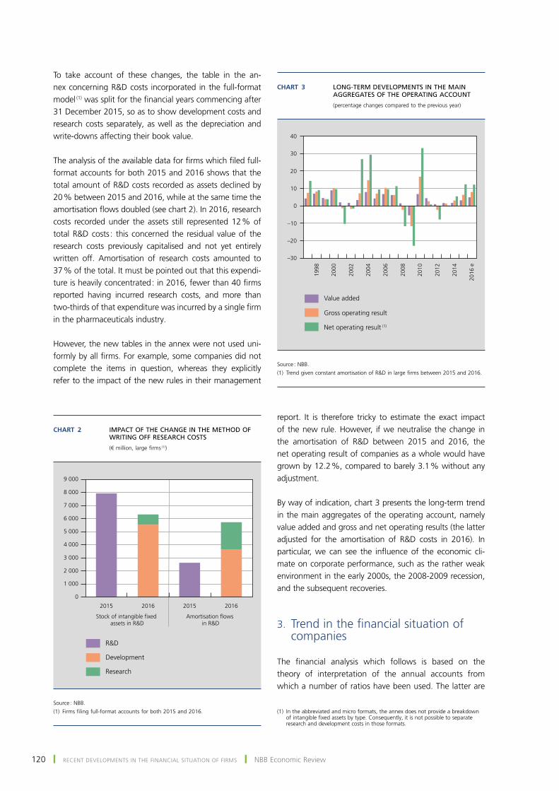
120 ❙ REcENt DEvElopmENtS IN tHE fINANcIAl SItuAtIoN of fIRmS ❙ NBB Economic Review
to take account of these changes, the table in the an‑nex concerning R&D costs incorporated in the full‑format model (1) was split for the financial years commencing after 31 December 2015, so as to show development costs and research costs separately, as well as the depreciation and write-downs affecting their book value.
The analysis of the available data for firms which filed full-format accounts for both 2015 and 2016 shows that the total amount of R&D costs recorded as assets declined by 20 % between 2015 and 2016, while at the same time the amortisation flows doubled (see chart 2). In 2016, research costs recorded under the assets still represented 12 % of total R&D costs : this concerned the residual value of the research costs previously capitalised and not yet entirely written off. Amortisation of research costs amounted to 37 % of the total. It must be pointed out that this expendi‑ture is heavily concentrated : in 2016, fewer than 40 firms reported having incurred research costs, and more than two-thirds of that expenditure was incurred by a single firm in the pharmaceuticals industry.
However, the new tables in the annex were not used uni‑formly by all firms. For example, some companies did not complete the items in question, whereas they explicitly refer to the impact of the new rules in their management
report. It is therefore tricky to estimate the exact impact of the new rule. However, if we neutralise the change in the amortisation of R&D between 2015 and 2016, the net operating result of companies as a whole would have grown by 12.2 %, compared to barely 3.1 % without any adjustment.
By way of indication, chart 3 presents the long-term trend in the main aggregates of the operating account, namely value added and gross and net operating results (the latter adjusted for the amortisation of R&D costs in 2016). In particular, we can see the influence of the economic cli‑mate on corporate performance, such as the rather weak environment in the early 2000s, the 2008-2009 recession, and the subsequent recoveries.
3. Trend in the financial situation of companies
The financial analysis which follows is based on the theory of interpretation of the annual accounts from which a number of ratios have been used. The latter are
(1) In the abbreviated and micro formats, the annex does not provide a breakdown of intangible fixed assets by type. Consequently, it is not possible to separate research and development costs in those formats.
Chart 2 IMPACT OF THE CHANGE IN THE METHOD OF WRITING OFF RESEARCH COSTS
(€ million, large firms (1))
2015 2016 2015 2016
R&D
Development
Research
Stock of intangible fixed assets in R&D
Amortisation flows in R&D
0
1 000
2 000
3 000
4 000
5 000
6 000
7 000
8 000
9 000
Source : NBB.(1) Firms filing full-format accounts for both 2015 and 2016.
Chart 3 LONG-TERM DEVELOPMENTS IN THE MAIN AGGREGATES OF THE OPERATING ACCOUNT
(percentage changes compared to the previous year)
1998
2000
2002
2004
2006
2008
2010
2012
2014
–30
–20
–10
0
10
20
30
40
2016
e
Value added
Gross operating result
Net operating result (1)
Source : NBB.(1) Trend given constant amortisation of R&D in large firms between 2015 and 2016.

121December 2017 ❙ REcENt DEvElopmENtS IN tHE fINANcIAl SItuAtIoN of fIRmS ❙
defined in detail in Annex 1. The ratios are presented mainly in the form of globalisations and medians. the globalisation of a ratio divides the sum of the numerators of all companies by the sum of their denominators. the median is the central value in an ordered distribution : for a given ratio, 50 % of companies will have a ratio which is above the median and 50 % will have a ratio below it. The two measures are complementary because they meet different needs. By taking account of the weight of each observation in the numerator and the denominator, the globalisation mainly reflects the situation of the largest firms. Conversely, the median reflects the trend for the whole distribution as it is influenced equally by all firms, regardless of their size.
3.1 Profitability
In this article, profitability is studied according to four ratios (see chart 4) : the margin on sales (calculated for large firms only), the return on the operating assets, the return on the total assets and the return on equity.
the return on sales is traditionally measured by the net margin on sales. That provides an indication of the firm’s ability to make a profit on its sale proceeds after deducting all the operating costs, excluding financial and exceptional items and taxes. Since the change in the operating result which appears in the numerator is distorted in 2016 by the modification of the accounting rules on the amortisation of research costs, we also show the gross indicator which reports the operating profit before non-cash expenses. the return on the operating assets compares the recurring operating result (1) with the short- and long-term operating assets. this ratio expresses the commercial performance in relation to the balance sheet items directly allocated to operating activities. the return on the total assets, or economic return, measures the net result before tax and financing costs in relation to the whole of the resources used, i.e. the total assets. The profit is considered before taxes and financial charges so as to be unaffected by the tax system and the financing policy. The ratio can be cal‑culated excluding exceptional – or non‑recurring – results if the focus is on the normal business result. the return on equity, or financial return, divides the profit after tax by the total equity. It indicates the return that shareholders obtain from the activities of the business.
the ratios for the sales margin and the return on the operat‑ing assets, which have the operating result as the numera‑tor, both assess the commercial performance of firms, one on the scale of large companies only and the other for all firms. While the levels of these two indicators are differ-ent, they display a similar trend. In the globalised data,
the 2008-2009 recession led to a fall in the ratios, which subsequently stabilised between 2011 and 2014 at well be‑low their pre-crisis levels. A recovery which began in 2015 was confirmed in 2016 thanks to falling commodity prices – despite a dip followed by a revival during 2016 – and a favourable exchange rate against the uS dollar combined with a reduction in labour costs. Nevertheless, the median indicators present a less favourable picture for the past two years : for example, the ratio measuring the gross return on the operating assets regained a level comparable to the pre-crisis figure from 2010, but has hardly changed since then, showing that all firms did not benefit equally from the recent improvement in the economic environment.
the ratios for the return on total assets and the return on equity (2) broaden the performance concept considered by including the financial and exceptional results. They, too, exhibit similar profiles, although the second is more volatile than the first since the result is compared to a lower denominator. The rate of return on the total assets in globalised terms has dropped by around 3 percentage points below the pre-crisis levels, hovering around 5 % since 2013. Over the long term, part of the decline is due to the influence of the exceptional results, which made a substantial contribution towards supporting corporate profitability in the pre-crisis years – up to 1.7 percentage points in 2005 – whereas that contribution has been fairly modest since 2013. It should be noted that the median ratios, whether or not they include the exceptional results, have been remarkably stable over time – with a standard deviation of just 0.2 percentage point over the past fifteen years – and that the divergences between the globalised and median series (which were very large in the first ten years of the period under review) have since been totally eliminated, as the values recorded have been in the region of 5 % since 2013, whichever concept is used.
Although they show profitability in different forms, the ratios which have just been discussed are (very) closely correlated : after winsorisation at percentiles 5 and 95 (an essential process owing to some extreme values) (3), the correlation coefficients fall between +0.53 and +0.94 de‑pending on the pairs of ratios considered. By way of indi‑cation, chart 5 shows two examples of scatter plots for a random sample of 1 000 sets of annual accounts. Apart from the clearly positive correlation, this chart reveals
(1) Transposition of Directive 2013 / 34 / EU led to reallocation of the exceptional elements between operating income / expenditure and financial income / expenditure in the profit and loss account. These non-recurring elements relating to operating or financing activities nevertheless appear under a specific item so that it is still possible to separate them from the recurring elements, which are the only ones taken into consideration here.
(2) Annex 3 presents a sectoral breakdown of the results obtained for the return on equity ratio.
(3) Reminder : winsorisation at percentiles 5 and 95 means that values below percentile 5 are set at percentile 5, while values above percentile 95 are set at percentile 95.

122 ❙ REcENt DEvElopmENtS IN tHE fINANcIAl SItuAtIoN of fIRmS ❙ NBB Economic Review
certain specific features. For instance, in the vast majority of cases, the net margin on sales is, as one would expect, lower than the gross margin : however, a very few firms do record a higher net margin, due to withdrawals from provi‑sions and / or write-downs. The impact of winsorisation is also evident, particularly for the return on equity which, after
that process, shows a minimum of –66 % and a maximum of +88 %. This ratio is particularly prone to abnormal values, mainly on account of its denominator, which may be very slightly positive as a result of losses carried forward (1).
Chart 4 PROFITABILITY (1)
(in % : all firms, unless otherwise stated)
2002
2004
2006
2008
2010
2012
2014
0
1
2
3
4
5
6
7
8
9
10
2002
2004
2006
2008
2010
2012
2014
0
1
2
3
4
5
6
7
8
9
10
2002
2004
2006
2008
2010
2012
2014
0
2
4
6
8
10
12
14
16
2002
2004
2006
2008
2010
2012
2014
0
2
4
6
8
10
12
14
16
Gross margin
MARGIN ON SALES (1)
2016
e
Globalised values Globalised values
Median values Median values
Net margin Total
NET RETURN ON TOTAL ASSETS BEFORE TAX AND FINANCIAL CHARGES
2016
e
Globalised values Globalised values
Median values Median values
Total excluding exceptional results
Gross return
NET RETURN ON OPERATING ASSETS (1)
2016
e
Globalised values Globalised values
Median values Median values
Net return Total
NET RETURN ON EQUITY AFTER TAX20
16 e
Globalised values Globalised values
Median values Median values
Total excluding exceptional results
Source : NBB.(1) The margin on sales ratios are calculated only for large firms. The gross concepts are calculated before deduction of depreciation, write-downs and contingency provisions in
the numerator, while the net concepts are calculated after deduction of those expenses.
(1) The ratio is not calculated in the case of negative equity.

123December 2017 ❙ REcENt DEvElopmENtS IN tHE fINANcIAl SItuAtIoN of fIRmS ❙
3.2 Solvency
Solvency indicates the ability of firms to meet their short‑ and long‑term liabilities. the main measurement of solvency is the degree of financial independence, i.e. the ratio between the equity and the total liabilities. An alter‑native way of measuring solvency is via the degree of self-financing : here, the numerator comprises only the reserves and results carried forward, while the denominator is unchanged. This ratio reflects the firm’s past profitability, its policy on the allocation of the results and, indirectly, its age. By nature, the trend in the degree of self-financing mirrors that in the degree of financial independence because the reserves represent a substantial part of the equity.
As chart 6 shows, the degree of financial independence has clearly improved over the past 15 years, both for large firms – whose ratios are normally higher – and for SmEs (1). During the second half of the 2000s, the long-term tendency was reinforced by the introduction of the tax allowance for risk capital ("notional interest"). That allowance attracted a massive inflow of foreign capital into Belgium, which primarily benefited very large companies, especially in the "head office activities" branch, which is excluded from this analysis because the social object of these undertakings is primarily financial. However, the phasing-in of restrictions on the allowance combined with the fall in interest rates significantly reduced the scheme’s attraction in recent years. That is reflected in particular in
the globalised ratio for large firms, in decline since 2013, notably as a result of a number of large‑scale reductions in capital. In contrast, in the SmEs, the globalised ratio has stabilised at a high level in recent years, while the median ratio has displayed a marked increase, indicating a funda‑mental trend affecting most of these firms.
The picture concerning median values in SMEs was greatly influenced by the changes made in recent years in the tax treatment of liquidation surpluses. It should be remembered that the liquidation surplus broadly corresponds to the re‑tained earnings that a company accumulates and which are allocated to the owners in the event of liquidation. Those surpluses are regarded as dividends and are therefore subject to withholding tax. The tax rate applicable here used to be 10 %, but was increased to 25 % in October 2014, then 27 % in January 2016 and 30 % in January 2017.
In order to give companies time to adjust, the government introduced a transitional measure at the time of the 2014 increase, allowing companies – regardless of size – to remain eligible for the 10 % rate if they incorporated in their capital (2) the taxed reserves formed by no later than
Chart 5 SCATTER PLOTS OF PROFITABILITY RATIOS
(2015)
–80
–60
–40
–20
0
20
40
60
–40 –20 800 20 40 60
–40
–30
–20
–10
0
10
20
30
40
50
–80 –60 –40 –20 806040200 100
Net
mar
gin
on s
ales
Gross margin on salesN
et re
turn
on
tota
l ass
ets
Net return on equity
Source : NBB.
(1) Annex 4 presents a sectoral breakdown of the results obtained for the degree of financial independence.
(2) Under the transitional arrangement in Article 537 of the Income Tax Code, dividends corresponding to the reduction in the taxed reserves, of which the amount received was immediately added to the company capital and retained for a specified period (four years in the case of small firms, eight for large firms) still qualified for the reduced rate of 10 %.

124 ❙ REcENt DEvElopmENtS IN tHE fINANcIAl SItuAtIoN of fIRmS ❙ NBB Economic Review
31 March 2013, provided that this contribution is main‑tained for a minimum period. In many firms, this measure led to amounts placed in reserve being transferred to the company capital, influencing their degree of self-financing in 2013 and 2014.
The Programme Law of 19 December 2014 then per‑petuated the temporary measure, but only for small firms and in a slightly different form (1). Since the 2014 financial year, those firms have been allowed to allocate all or part of their profit after tax to a special reserve, called the "liquidation reserve", on which there is an immediate levy of 10 % (2). that reserve can be paid out with no additional levy in the event of liquidation : if it is paid out in the form of dividends before liquidation, a re‑duced rate of withholding tax applies to those dividends. The reduction is particularly large if the liquidation re‑serve is retained in the business for five years, since the withholding tax rate is then 5 % instead of 17 % other‑wise (3). A large number of SmEs evidently opted for the liquidation reserve scheme in 2015 and 2016, causing a sharp rise in the reserves – to the detriment of the pay‑ment of dividends – and hence an increase in the self‑financing and financial independence ratios. It is possible that new structural changes may be seen in the coming years, if firms opt for early distribution of these liquida‑tion reserves in the form of dividends. the forthcoming reform of corporation tax will doubtless also influence firms’ behaviour (4).
Finally, it must be said that while the medians and glo‑balised data indicate that solvency is tending to improve, examination of the whole distribution tempers that finding. Chart 7, which shows the whole distribution of financial independence in the form of box plots, reveals particularly wide variations in the solvency position of firms : by way of indication, in 2016, the 9th decile of financial independence stood at 88 % while the figure for the 1st decile was –29 %. The chart also shows that the solvency gains applied mainly to the most solvent population strata : while the 3rd quartile gained 9 points between 2002 and 2016, the 1st quartile only saw a 2 point increase. The 1st decile lost 13 points over the same period, indicating that a significant section of the popula‑tion lost ground, in contrast to the majority upward trend. Note that 17 % of firms have negative equity, which is a significant financial warning light. However, some of the
(1) According to the Law’s explanatory memorandum, it was decided to keep this alternative arrangement "in response to complaints from many self-employed persons pursuing their activities in the form of a company who expected to be able to pay out their reserves on liquidation at a rate of 10 % in the future". See the draft Programme Law of 28 November 2014 (parliamentary paper DOC 54 0672 / 001, Belgian Chamber of Representatives).
(2) This scheme came into force from the 2014 financial year. A catch-up measure was also introduced for earnings retained in the business and relating to the 2012 and 2013 financial years ; allowing firms to add those earnings to the liquidation reserve too.
(3) Originally, this tax rate stood at 15 %. It was increased to 17 % for reserves formed during a taxable period concerning the 2017 tax year or an earlier year, and to 20 % for reserves relating to the 2018 tax year at the earliest.
(4) According to government statements, the corporate tax reform, among other measures, will lower the rate of tax on companies, cutting the nominal rate from 33 % to 29 % from January 2018, then to 25 % from the following year. The rate applicable to SMEs will actually be 20 % for the first € 100 000.
Chart 6 SOLVENCY
(in %)
2002
2004
2006
2008
2010
2012
2014
25
30
35
40
45
50
2002
2004
2006
2008
2010
2012
2014
0
5
10
15
20
25
Large firms
DEGREE OF FINANCIAL INDEPENDENCE
2016
e
Globalised values Globalised values
Median values Median values
SMEs
2016
e
DEGREE OF SELF-FINANCING
Source : NBB.
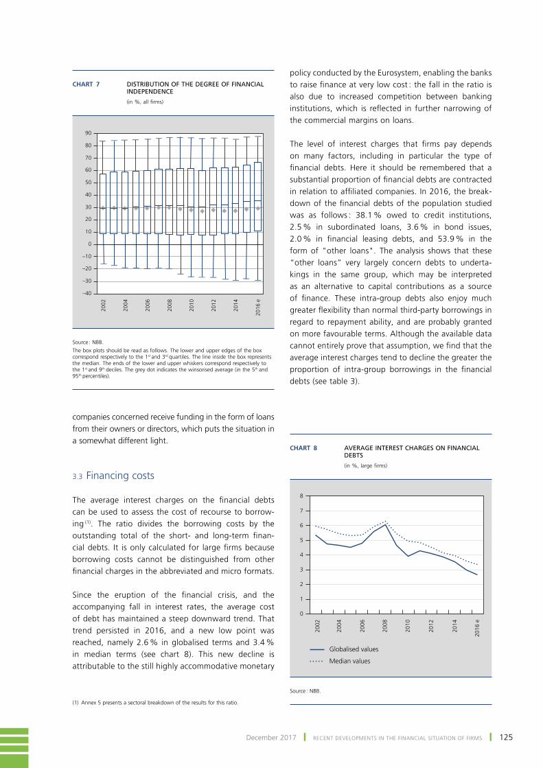
125December 2017 ❙ REcENt DEvElopmENtS IN tHE fINANcIAl SItuAtIoN of fIRmS ❙
companies concerned receive funding in the form of loans from their owners or directors, which puts the situation in a somewhat different light.
3.3 financing costs
The average interest charges on the financial debts can be used to assess the cost of recourse to borrow-ing (1). The ratio divides the borrowing costs by the outstanding total of the short- and long-term finan‑cial debts. It is only calculated for large firms because borrowing costs cannot be distinguished from other financial charges in the abbreviated and micro formats.
Since the eruption of the financial crisis, and the accompanying fall in interest rates, the average cost of debt has maintained a steep downward trend. That trend persisted in 2016, and a new low point was reached, namely 2.6 % in globalised terms and 3.4 % in median terms (see chart 8). This new decline is attributable to the still highly accommodative monetary
policy conducted by the Eurosystem, enabling the banks to raise finance at very low cost : the fall in the ratio is also due to increased competition between banking institutions, which is reflected in further narrowing of the commercial margins on loans.
The level of interest charges that firms pay depends on many factors, including in particular the type of financial debts. Here it should be remembered that a substantial proportion of financial debts are contracted in relation to affiliated companies. In 2016, the break‑down of the financial debts of the population studied was as follows : 38.1 % owed to credit institutions, 2.5 % in subordinated loans, 3.6 % in bond issues, 2.0 % in financial leasing debts, and 53.9 % in the form of "other loans". The analysis shows that these “other loans” very largely concern debts to underta‑kings in the same group, which may be interpreted as an alternative to capital contributions as a source of finance. These intra-group debts also enjoy much greater flexibility than normal third-party borrowings in regard to repayment ability, and are probably granted on more favourable terms. Although the available data cannot entirely prove that assumption, we find that the average interest charges tend to decline the greater the proportion of intra-group borrowings in the financial debts (see table 3).
Chart 7 DISTRIBUTION OF THE DEGREE OF FINANCIAL INDEPENDENCE
(in %, all firms)
— — — — — — —— — — — — — — —
— — — — — — — — — — — — — — —
2002
2004
2006
2008
2010
2012
2014
–40
–30
–20
–10
0
10
20
30
40
50
60
70
80
90
2016
e
Source : NBB.The box plots should be read as follows. The lower and upper edges of the box correspond respectively to the 1st and 3rd quartiles. The line inside the box represents the median. The ends of the lower and upper whiskers correspond respectively to the 1st and 9th deciles. The grey dot indicates the winsorised average (in the 5th and 95th percentiles).
(1) Annex 5 presents a sectoral breakdown of the results for this ratio.
Chart 8 AVERAGE INTEREST CHARGES ON FINANCIAL DEBTS
(in %, large firms)
2002
2004
2006
2008
2010
2012
2014
0
1
2
3
4
5
6
7
8
Globalised values
Median values
2016
e
Source : NBB.
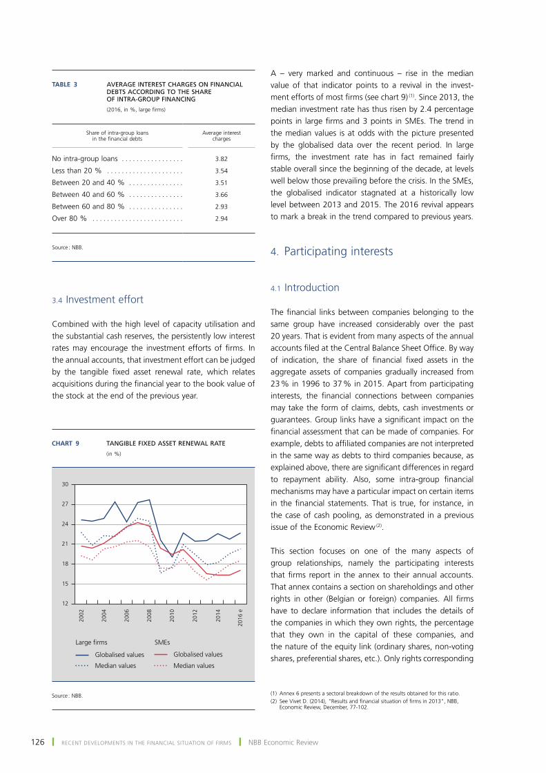
126 ❙ REcENt DEvElopmENtS IN tHE fINANcIAl SItuAtIoN of fIRmS ❙ NBB Economic Review
3.4 Investment effort
Combined with the high level of capacity utilisation and the substantial cash reserves, the persistently low interest rates may encourage the investment efforts of firms. In the annual accounts, that investment effort can be judged by the tangible fixed asset renewal rate, which relates acquisitions during the financial year to the book value of the stock at the end of the previous year.
A – very marked and continuous – rise in the median value of that indicator points to a revival in the invest‑ment efforts of most firms (see chart 9) (1). Since 2013, the median investment rate has thus risen by 2.4 percentage points in large firms and 3 points in SMEs. The trend in the median values is at odds with the picture presented by the globalised data over the recent period. In large firms, the investment rate has in fact remained fairly stable overall since the beginning of the decade, at levels well below those prevailing before the crisis. In the SMEs, the globalised indicator stagnated at a historically low level between 2013 and 2015. The 2016 revival appears to mark a break in the trend compared to previous years.
4. participating interests
4.1 Introduction
The financial links between companies belonging to the same group have increased considerably over the past 20 years. That is evident from many aspects of the annual accounts filed at the Central Balance Sheet Office. By way of indication, the share of financial fixed assets in the aggregate assets of companies gradually increased from 23 % in 1996 to 37 % in 2015. Apart from participating interests, the financial connections between companies may take the form of claims, debts, cash investments or guarantees. Group links have a significant impact on the financial assessment that can be made of companies. For example, debts to affiliated companies are not interpreted in the same way as debts to third companies because, as explained above, there are significant differences in regard to repayment ability. Also, some intra-group financial mechanisms may have a particular impact on certain items in the financial statements. That is true, for instance, in the case of cash pooling, as demonstrated in a previous issue of the Economic Review (2).
this section focuses on one of the many aspects of group relationships, namely the participating interests that firms report in the annex to their annual accounts. that annex contains a section on shareholdings and other rights in other (Belgian or foreign) companies. All firms have to declare information that includes the details of the companies in which they own rights, the percentage that they own in the capital of these companies, and the nature of the equity link (ordinary shares, non-voting shares, preferential shares, etc.). Only rights corresponding
Table 3 AVERAGE INTEREST CHARGES ON FINANCIAL DEBTS ACCORDING TO THE SHARE OF INTRA-GROUP FINANCING
(2016, in %, large firms)
Share of intra-group loans in the financial debts
Average interest charges
No intra-group loans . . . . . . . . . . . . . . . . . 3.82
Less than 20 % . . . . . . . . . . . . . . . . . . . . . 3.54
Between 20 and 40 % . . . . . . . . . . . . . . . 3.51
Between 40 and 60 % . . . . . . . . . . . . . . . 3.66
Between 60 and 80 % . . . . . . . . . . . . . . . 2.93
Over 80 % . . . . . . . . . . . . . . . . . . . . . . . . . 2.94
Source : NBB.
(1) Annex 6 presents a sectoral breakdown of the results obtained for this ratio.(2) See Vivet D. (2014), "Results and financial situation of firms in 2013", NBB,
Economic Review, December, 77-102.
Chart 9 TANGIBLE FIXED ASSET RENEWAL RATE
(in %)
2002
2004
2006
2008
2010
2012
2014
12
15
18
21
24
27
30
Large firms
2016
e
Globalised values Globalised values
Median values Median values
SMEs
Source : NBB.

127December 2017 ❙ REcENt DEvElopmENtS IN tHE fINANcIAl SItuAtIoN of fIRmS ❙
to at least 10 % of the company’s subscribed capital are deemed to be declared.
To obtain an overall view of the data collected by the Central Balance Sheet Office, the results presented in this section cover all firms filing annual accounts, i.e. commercial companies filing accounts in standardised formats, but also banks, insurance companies, NpIs and foundations. this set is therefore larger than the population studied in the preceding sections of the article.
Unlike the other items in the financial statements, the data on shareholdings do not really lend them‑selves to quality checks by the Central Balance Sheet Office. Before the actual analysis, a lengthy exploratory exercise was therefore conducted on the gross data. Overall, while some imperfections were found, they were confined to a small number of cases so that the results can be considered generally reliable.
one of the checks conducted during the exploratory phase concerned consistency between the annex on shareholdings and the corresponding asset items, i.e. the financial fixed as‑sets but also occasionally cash investments. It was found that 97 % of companies declaring shareholdings in the annex also reported corresponding assets on the balance sheet. Moreover, there was generally an explanation for the occa‑sional divergence. For instance, total write-downs may be re‑corded on financial fixed assets (e.g. if the company in which a stake is held has gone bankrupt or into liquidation), so that the net book value of the shares is zero. moreover, in theory, the concept of a participating interest is based primarily on the power to exercise control over the undertaking. While that control is usually associated with a shareholding, it may also be exercised in other ways, e.g. if a company has the power to appoint the directors or to exercise decisive influ‑ence over the management of a third undertaking.
4.2 long‑term trends
During the 20 years under review (1), the number of participating interest links more than doubled, from 36 570 in 1996 to 79 258 in 2015 (see chart 10). For 2015, the breakdown of the links is as follows ac‑cording to the type of annual accounts of the owner company : 30 202 links were declared in the full-format model, 46 876 in the abbreviated formats and 2 180 in other types of annual accounts (mainly filed by banks, insurers, NPIs and foundations).
Chart 10 NUMBER OF SHAREHOLDING LINKS BY TYPE OF ACCOUNTS FORMAT FILED BY THE INVESTOR UNDERTAKING
1997
1999
2001
2003
2005
2007
2009
2011
2013
2015
Full format
Abbreviated format
Other (1)
0
10 000
20 000
30 000
40 000
50 000
60 000
70 000
80 000
90 000
79 258
36 570
Source : NBB.(1) Mainly annual accounts filed by banks, insurers, NPIs and foundations.
The number of firms with at least one shareholding link also displayed an upward trend over the last 20 years as a whole, reaching 95 018 in 2015 (see chart 11).
Chart 11 NUMBER OF COMPANIES WITH AT LEAST ONE SHAREHOLDING LINK
1997
1999
2001
2003
2005
2007
2009
2011
2013
2015
Exclusively investee companies
Combined investor and investee companies
Exclusively investor companies
0
20 000
40 000
60 000
80 000
100 000 95 018
44 069
Source : NBB.(1) The period studied covers the financial years from 1996 to 2015, as 2016 was
not complete when this article went to press.

128 ❙ REcENt DEvElopmENtS IN tHE fINANcIAl SItuAtIoN of fIRmS ❙ NBB Economic Review
That figure can be broken down into 30 391 firms that were purely investors, 55 653 that were purely inves‑tees, and 8 974 that were both investors and investees. It should be noted that while the number of investor companies is considered exhaustive – since we have infor‑mation on all entities operating in Belgium – that is not the case for investee companies, as the database cannot identify the Belgian companies in which foreign counter‑parties own a stake.
While group relationships have developed consistently in absolute terms, we must point out that over the same period many firms were set up and, taking all formats together, the number of annual accounts filed by companies at the Central Balance Sheet Office increased considerably, from 215 065 in 1996 to 405 633 in 2015. The question was therefore whether, in proportionate terms, there are more group links nowadays than in the past. As is evident from table 4, the proportion of companies with at least one shareholding link has indeed increased over time, but to a relatively lesser degree : it edged upwards from 12.1 % in 1996 to 15.2 % in 2015 in the case of abbreviated formats, and from 64.1 to 71.2 % for full formats. Those proportions are likely to change in the future, following implementation of the EU Directive (see above). Another point is that, in the case of the abbreviated formats, the analysis is distorted by the fact that the central Balance Sheet Office collects annual accounts from all Belgian firms operating in the form of a company : in practice, that in‑cludes a very large number of small companies which are unlikely to have participating interests, such as companies set up by self-employed workers.
Overall, this growth of connections between firms reflects the general trend towards an increase in the number of le‑gal structures, as firms have become more inclined to cre‑ate separate companies for each function or activity. While that trend has concerned all branches of activity, it has
been driven in particular by numerous companies set up in spheres which are, by nature, conducive to participating interests. This primarily concerns "business and other management consultancy activities" (NACE-BEL 70 220), a branch which includes companies whose object is to take part in the management of other businesses (1). It also concerns "head office activities" (NACE-BEL 70 100), comprising mainly holding companies or those performing financial functions inside groups of companies (in-house banks, cash-pooling companies, etc.). In addition, the real estate sector has likewise influenced the trend via the development of companies intended to operate and rent out properties : these real estate companies are generally firms in which other companies have a partici‑pating interest, whereas most companies in the other two branches hold participating interests themselves.
4.3 characteristics of shareholding links in 2015
Of the approximately 80 000 links identified in 2015, 66 % concerned companies based in Flanders, 18 % related to firms with their head office in Wallonia, and 17 % concerned firms based in Brussels. The Brussels companies have a participating interest profile which is clearly different from that of firms based in Flanders or Wallonia : the latter tend to have intra‑regional links – in flanders, both partners are based in the Flemish Region in 76 % of cases, while the figure for Wallonia is 70 % – whereas Brussels-based firms invest more outside their Region, and in particular abroad (see table 5). Thus, more than a third of the stakes owned by Brussels firms concern rights acquired in foreign under‑takings, while that proportion is around 20 % if the owner company is flemish or from Wallonia. this peculiarity is partly due to the Brussels economic fabric, comprising numerous head offices of international undertakings.
the foreign investee companies can also be broken down by country (2). As table 6 shows, these foreign companies originate primarily from the countries bordering on Belgium, i.e. France (6 %), the Netherlands (4 %), Luxembourg (2 %) and Germany (1 %). Then comes a wide variety of countries : altogether, Belgian companies owned participating interests in more than 177 countries in 2015, representing the great majority of countries in the world (the UN recognises just under 200 countries).
Table 4 PERCENTAGE OF COMPANIES WITH AT LEAST ONE SHAREHOLDING LINK, BY TYPE OF FORMAT FILED
(in %)
Financial year
Abbreviated formats
Full formats
1996 . . . . . . . . . . . . . . . . . . . 12.1 64.1
2015 . . . . . . . . . . . . . . . . . . . 15.2 71.2
Change (in percentage points) . . . . . +3.1 +7.0
Source : NBB.
(1) On the subject of management companies, see for example Herve L. (2012), Les sociétés de management en 2012, Pacioli n° 345, IPCF-BIBF, and Mormont H. (1999), La société de management et la jurisprudence des juridictions sociales, pacioli n° 52, Ipcf‑BIBf.
(2) Reminder : apart from a few exceptions, the investor companies are all incorporated under Belgian law.

129December 2017 ❙ REcENt DEvElopmENtS IN tHE fINANcIAl SItuAtIoN of fIRmS ❙
Another aspect of the shareholding links concerns their intensity. that can be measured, for instance, by the direct participation rate declared by the investor firms. To avoid double counting, we disregarded any declared indirect links (which reflect the additional control that a firm may exercise over a third company via its subsidiaries). It must be stressed that the direct participation rate does not give a perfect picture of the intensity of the links between firms. It can in fact be zero (as in the case of 2 % of links) if the firm does not own any shares in the third company but exercises indirect control via its subsidiaries (1). Also, if the
investor firm holds corporate rights of varying types (a situ‑ation that only concerns a small number of participating interests), it states various percentages for the same stake, making interpretation difficult.
A stake of at least 10 % in the investee equity implies a presumption of a participating interest, which is why – un‑less there is evidence to the contrary – once that threshold
Table 5 BREAKDOWN OF PARTICIPATING INTERESTS ACCORDING TO INVESTOR AND INVESTEE COMPANIES’ LOCATION
(in %)
Location of the investor company
Location of the investee company
Belgium
Abroad
Total
of which:
Flanders
Wallonia
Brussels
Flanders . . . . . . . . . . . . . . . . . . . . . 80.6 75.6 2.5 2.5 19.4 100
Wallonia . . . . . . . . . . . . . . . . . . . . 79.3 3.8 70.3 5.2 20.7 100
Brussels . . . . . . . . . . . . . . . . . . . . . 64.7 9.9 7.1 47.6 35.3 100
Belgium . . . . . . . . . . . . . . . . . . . . 79.0 10.6 52.7 15.7 21.0 100
Source : NBB.
(1) In many cases where the direct rate is missing, the reporting companies mention an indirect equity link, which exceeds 50 % in more than a third of cases.
Table 6 GEOGRAPHICAL BREAKDOWN OF INVESTEE COMPANIES
Country
Number of companies
Country
Number of companies
Country
Number of companies
Belgium . . . . . . . . . . . . . . . . . 49 031 Czech Republic . . . . . . . . . . . 201 Ireland . . . . . . . . . . . . . . . . . . 94
France . . . . . . . . . . . . . . . . . . 3 687 Brazil . . . . . . . . . . . . . . . . . . . 166 Bulgaria . . . . . . . . . . . . . . . . . 84
Netherlands . . . . . . . . . . . . . . 2 342 India . . . . . . . . . . . . . . . . . . . . 163 South Africa . . . . . . . . . . . . . 84
Luxembourg . . . . . . . . . . . . . 1 182 Portugal . . . . . . . . . . . . . . . . . 154 Denmark . . . . . . . . . . . . . . . . 80
Germany . . . . . . . . . . . . . . . . 761 Turkey . . . . . . . . . . . . . . . . . . 154 Austria . . . . . . . . . . . . . . . . . . 74
United States . . . . . . . . . . . . 641 Slovakia . . . . . . . . . . . . . . . . . 144 Greece . . . . . . . . . . . . . . . . . . 67
United Kingdom . . . . . . . . . . 583 Russia . . . . . . . . . . . . . . . . . . . 140 Japan . . . . . . . . . . . . . . . . . . . 65
Spain . . . . . . . . . . . . . . . . . . . 510 Hungary . . . . . . . . . . . . . . . . . 133 Cyprus . . . . . . . . . . . . . . . . . . 63
Poland . . . . . . . . . . . . . . . . . . 431 Sweden . . . . . . . . . . . . . . . . . 130 United Arab Emirates . . . . . . 58
Italy . . . . . . . . . . . . . . . . . . . . 389 Canada . . . . . . . . . . . . . . . . . 118 Argentina . . . . . . . . . . . . . . . 57
Hong Kong . . . . . . . . . . . . . . 323 Singapore . . . . . . . . . . . . . . . 107 Chile . . . . . . . . . . . . . . . . . . . . 57
Romania . . . . . . . . . . . . . . . . 248 Morocco . . . . . . . . . . . . . . . . 106 D.R. of Congo . . . . . . . . . . . 53
Switzerland . . . . . . . . . . . . . . 244 Australia . . . . . . . . . . . . . . . . 99 Ukraine . . . . . . . . . . . . . . . . . 52
China . . . . . . . . . . . . . . . . . . . 233 Mexico . . . . . . . . . . . . . . . . . . 98 Rest of the world . . . . . . . . . 1 156
Source : NBB.

130 ❙ REcENt DEvElopmENtS IN tHE fINANcIAl SItuAtIoN of fIRmS ❙ NBB Economic Review
is passed, a participating interest is mentioned in the ad- hoc annex.
If the investor company holds more than 50 % of the capi‑tal in another company, the latter is regarded de facto as a subsidiary. The Royal Decree of 12 September 1983 de-s cribes a subsidiary as "any other undertaking if the first undertaking is able, in fact or in law, to exercise decisive influence over the appointment of at least half of the directors of the second undertaking or over its manage‑ment policy, either by virtue of agreements or as a result of participating interests held in the second undertaking by the first, or indirectly via its direct or indirect subsidia ries". This means that, in practice, a firm may be classed as a subsidiary below the 50 % threshold if power of control is demonstrated. From the industrial point of view, it may make sense to acquire a majority stake in order to squeeze out a competitor, to ensure a supplier’s loyalty, to extend the customer base via a local player or to acquire technol-ogy needed to develop the business. From the financial point of view, a majority stake means control over the distribution of the profits made.
The Company Code describes an affiliated company as "any company other than a subsidiary in which another company holds a participating interest and can exert significant influence over its policy". That "significant" influence is presumed where the voting rights attached to
that participating interest represent 20 % or more of the capital of the investee company.
Chart 12 shows that most of the participating interests mentioned by firms in their annual accounts concern the parent-subsidiary relationships : 63 % of the links in fact relate to a stake of more than 50 % in the corporate rights. It should be noted that in almost half of cases, the participation rate is actually between 90 and 100 %. More generally, around 80 % of the links recorded exceed the 20 % threshold beyond which a "significant" influence is presumed to be exercised by the investor company. furthermore, it is evident that the shareholding links are closer if the investee company is foreign, since 73 % of the participating interests in companies based outside Belgian territory refer to subsidiaries in the legal sense, whereas the figure is 61 % for holdings in Belgian firms. We can conclude that companies which invest abroad are keener to exert a decisive influence over the investee company.
Finally, the sectoral breakdown of investor companies shows that a large proportion of them come under head offices, management companies and financial activities (see chart 13). That is logical, since those branches of activity primarily imply stakes in other companies. It should be pointed out that companies in these branches generally employ few workers and create relatively
Chart 12 INTENSITY OF THE DIRECT SHAREHOLDING LINK
(in %)
12 %
25 %
17 %
46 %
13 %
18 %
43 %
9 %
18 %
15 %
58 %26 %
ALL PARTICIPATING INTERESTS
Majority stakes :
PARTICIPATING INTERESTS IN BELGIAN COMPANIES
PARTICIPATING INTERESTS IN FOREIGN COMPANIES
Less than 10 %
From 10 to 50 %
From 50 to 90 %
90 % or more
Source : NBB.

131December 2017 ❙ REcENt DEvElopmENtS IN tHE fINANcIAl SItuAtIoN of fIRmS ❙
little value added since they are usually set up for legal, financial or tax reasons.
conversely, the investee companies are much more often found in the traditional branches of the Belgian economy (such as industry, trade, construction, etc.) and they also employ far more staff, on average. It should be noted that the annual accounts of many large commercial or industrial firms nowadays exhibit a hybrid character, with assets con‑sisting mainly of financial fixed assets, on the one hand, and a profit and loss account which is still largely determined by the operating result (and hence by production activities).
4.4 Groups of firms
As stated above, the basic data come from the annual accounts of the investor companies, which declare the companies in which they hold participating interests, i.e. the investee companies. It should be remembered that the annual accounts do not contain any usable data on the shareholders of the company filing the accounts. One of the aims of this study was therefore to cross-check the initial data in order to identify any investor company shareholders in the other annual accounts so as ultimately to reconstruct groups of firms.
For example, if we have the annual accounts of companies A, D, E and F for which the data on participating interests are as follows :
– Annual accounts of company A : A → B ("A declares a stake in B")
A → c– Annual accounts of company D : D → A– Annual accounts of company E : E → D
E → A– Annual accounts of company F : F → c
By combining the data from these four sets of annual accounts we can deduce the diagram shown below, indicating the links. Among other things, this tells us about any firms owning the original investor companies (i.e. A, D, E and F) and the indirect links (e.g. the link between E and B which passes via A).
AB
CF
D
E
By extending this logic to all the annual accounts and levels of participating interest, it was possible, via a number of IT processes, to reconstruct groups of firms. For each firm, the group comprises all the companies in a chain of participating interests leading up or down to the firm, i.e. the companies with a direct or indirect ownership link with the firm, either upstream or down‑stream. If we look at the example of the above dia‑gram, this means that group A comprises firms B, C, D and E. Conversely, firm F is not part of group A because it does not figure in a chain of links leading up or down
Chart 13 SECTORAL BREAKDOWN OF FIRMS WITH AT LEAST ONE SHAREHOLDING LINK
19.2 %
17.9 %
4.3 %
15.7 %3.7 %
5.1 %
12.1 %
9.1 %
3.9 %1.8 %
7.1 %
Head offices and holding companies
Management consultancy
Finance, banking and insurance
Other business services
EXCLUSIVELY INVESTOR COMPANIES
Manufacturing industry
Construction
Trade
Real estate
Transport and storage
Information and communication
Other
2.0 %3.3 %3.8 %
12.3 %
9.9 %
11.4 %
23.7 %
11.3 %
4.3 %
4.3 %
13.6 %
EXCLUSIVELY INVESTEE COMPANIES
12.9 %
7.6 %
7.3 %
10.8 %
10.4 %8.4 %
16.4 %
10.6 %
5.0 %
3.9 %6.7 %
COMBINED INVESTOR AND INVESTEE COMPANIES
Source : NBB.

132 ❙ REcENt DEvElopmENtS IN tHE fINANcIAl SItuAtIoN of fIRmS ❙ NBB Economic Review
to A. By the same logic, group c does include f, just as it does A, D and E, whereas B is excluded.
one of the aspects investigated concerns the size of the groups thus formed. For a given firm, the group size was defined as the total number of firms upstream and / or downstream. The threshold defining whether or not participating interests are taken into consideration has a significant influence on group size : if we set the threshold at 0 %, i.e. if we take account of all the participating interests recorded, we obtain bigger groups than if we set the threshold at 50 %, for example. However, a 50 % threshold gives us more cohesive groups as the firms are connected by majority stakes from one end of chain of holdings to the other.
Table 7 presents the breakdown of the firms according to the size of their group, for four different thresholds : 0, 10, 20 and 50 %. For example, at the 20 % threshold, 53 752 firms are connected either upstream or down‑stream with one other firm by a direct link extending to 20 % or more. Conversely, 13 firms form part of a group of more than 200 firms. The main conclusion to be drawn from the table is that the vast majority of companies belong to small groups, while a minority form part of large groups. It should be noted that this conclusion concerns the data available from the Central Balance Sheet Office, which are
by nature incomplete. for one thing, they do not contain any information on stakes held by foreign companies in Belgian companies. Also, while we know the stakes held by Belgian companies in foreign companies, the chain ends at that stage, whereas those foreign companies may in turn hold stakes in other companies. These two points explain why the large groups identified are mainly Belgian.
4.5 participating interests and risk of default
This section discusses some first findings on the link between group relationships and financial risk. The analysis is based on the identification of failing companies : a company is considered to be failing if it is subject to bankruptcy proceedings within three years after the closing date of its annual accounts (1). the analysis concerned the annual accounts for the 2013 financial year, and hence failures occurring in 2014, 2015 and 2016. The default rates seen on that basis can be interpreted as an estimate of the risk of bankruptcy within three years.
Chart 14 presents the observed default rates according to the characteristics of the groups of firms as defined above. the main conclusion is that, all other things being equal, (a) the default risk is considerably lower for com‑panies forming part of a group, especially in the case of investor companies, and (b) the default risk declines as the group size increases. these conclusions are valid for the great majority of branches in the economy. Admittedly, the differences in the rates may seem minor at first sight, owing to the low percentage of bankruptcies recorded each year in Belgium (2). Nonetheless, the rate drops by more than half between individual firms (2.35 %) and investor companies (1.03 %), for example. Similarly, the rate is close to zero for groups comprising more than ten companies.
The group variables were also tested in the multivariate environment of the financial health indicator used by the Central Balance Sheet Office in its company files. Those first tests showed that the addition of such variables to the existing model improves its predictive quality. More detailed studies are therefore needed on this subject.
Table 7 BREAKDOWN OF FIRMS ACCORDING TO THE SIZE OF THEIR GROUP
(number of firms ; firms with at least one shareholding link in 2015)
Total number of firms upstream and / or downstream
Threshold
0 %
10 %
20 %
50 %
0 . . . . . . . . . . . . . . . . . . . . . 0 5 218 9 235 23 679
1 . . . . . . . . . . . . . . . . . . . . . 54 384 54 172 53 752 49 523
2 . . . . . . . . . . . . . . . . . . . . . 16 467 16 257 15 770 12 397
3 . . . . . . . . . . . . . . . . . . . . . 7 789 6 944 6 362 4 252
4 . . . . . . . . . . . . . . . . . . . . . 4 341 3 856 3 444 1 909
5 . . . . . . . . . . . . . . . . . . . . . 2 586 2 160 1 831 982
From 6 to 10 . . . . . . . . . . 5 429 4 100 3 107 1 495
From 11 to 20 . . . . . . . . . 2 631 1 592 1 028 537
From 21 to 50 . . . . . . . . . 1 091 555 407 211
From 51 to 100 . . . . . . . . 183 118 56 27
From 101 to 200 . . . . . . . 75 28 13 3
Over 200 . . . . . . . . . . . . . . 42 18 13 3
Total . . . . . . . . . . . . . . . . . 95 018 95 018 95 018 95 018
Source : NBB.
(1) This is the definition used in developing the financial health indicator included in the Central Balance Sheet Office company files.
(2) It is a peculiarity of most risk analyses that they only predict uncommon events.

133December 2017 ❙ REcENt DEvElopmENtS IN tHE fINANcIAl SItuAtIoN of fIRmS ❙
conclusion
The transposition into Belgian law of the EU Directive on fi‑nancial statements had a significant impact on the statistical interpretation of the annual accounts. The new provisions lead among other things to a considerable reform of the concepts of large and small firms within the meaning of the Company Code : they also modify the content of the annual accounts and the accounting treatment of certain items, such as research costs and exceptional results. these new provisions applicable to financial years commencing after 31 December 2015 create an unprecedented break in the Central Balance Sheet Office data series.
Some general lessons can still be drawn from the annual accounts relating to 2016. If we neutralise the impact of the change in the method of amortising research costs and the influence of certain one-off operations by multinationals which have no effect on real economic activity, the growth of the aggregate operating result was very stable in 2016, in both gross and net terms. That stability reflects an economic environment which combines mo derate activity growth with a favou rable trend in the main costs that firms incur (notably wages and commodity purchases). Overall, profitability also remained fairly stable in 2016 : while most of the profitability ratios were up slightly in globalised terms, there was hardly any improvement in the distribution measurements.
As regards solvency, a marked rise in the median ratios of SmEs has been the main feature in recent years. this
fundamental trend was evidently due to the changes in the tax treatment of liquidation surpluses, encouraging small firms to retain their taxed profits in house, first in the form of company capital and then in the form of special "liqui‑dation" reserves. While the main solvency figures reflect a steady improvement, it must be remembered that 17 % of the firms considered are in a negative equity situation, and that is an important financial warning light. The bank‑ruptcy statistics also point to renewed vulnerability in recent months : after three years of decline, the number of bank‑ruptcies began rising again from the third quarter of 2016.
In accordance with the trend evident since the eruption of the financial crisis, interest charges dropped further in 2016, in the context of a still highly accommoda‑tive monetary policy. Combined with the high level of capacity utilisation and the substantial cash reserves, the persistently low interest rates may encourage firms to invest. In that regard, it seems that the tangible fixed asset renewal rate of most firms, though still sig‑nificantly below the levels prevailing before the 2008-2009 recession, has been tending to pick up for several years now.
The last part of the article sheds light on the equity relationships between firms as declared in the annex to their annual accounts. Among the main conclusions derived from that analysis, we find that shareholding links are generally close : in almost two-thirds of cases, majority stakes are held. We also find that group
Chart 14 DEFAULT RISK ACCORDING TO PARTICIPATING INTERESTS
(default rate recorded at three years for companies filing annual accounts relating to the 2013 financial year)
0 0 1 2 3 4 5Individualcompanies(no link)
Exclusivelyinvestee
companies
Exclusivelyinvestor
companies
Combinedinvestee and
investorcompanies
0.0
0.5
1.0
1.5
2.0
2.5
(no links)
(links <
20 %)
6 to 10 11 to 20 Over20
COMPANY CHARACTERISTICS GROUP SIZE (AT THE 20 % THRESHOLD)
0.0
0.5
1.0
1.5
2.0
2.5
Source : NBB.

134 ❙ REcENt DEvElopmENtS IN tHE fINANcIAl SItuAtIoN of fIRmS ❙ NBB Economic Review
relationships have intensified over the past 20 years, reflecting a general trend towards a multiplicity of legal structures, as firms have become more inclined to cre‑ate separate companies for each function or activity. While that trend has concerned all branches of activity, it has been driven in particular by numerous companies set up in spheres which are, by nature, conducive to participating interests. This primarily concerns "man‑agement" companies, as well as head offices and holding companies. the companies in these branches generally employ few workers and create relatively little value added, because they are usually set up for legal, financial or tax reasons. Conversely, in the traditional branches of the Belgian economy (such as industry, trade, construction, etc.), investor companies employ far more staff, on average. It should be noted that the annual accounts of many large commercial or industrial
firms nowadays exhibit a hybrid character, with assets consisting mainly of financial fixed assets but a profit and loss account which is still largely determined by the operating result (and hence by production activities).
By combining the original data declared by firms, the analysis also enables us to reconstruct groups of companies. In particular, this work shows that the great majority of companies with participating interests belong to very small groups, while a minority of firms are part of very large groups. Finally, some initial find‑ings are discussed regarding the relationship between participating interests and financial risks. In this respect, we find that the risk of bankruptcy is significantly lower for companies forming part of a group, especially in the case of investor companies, and that this risk tends to decline as group size increases.

135December 2017 ❙ REcENt DEvElopmENtS IN tHE fINANcIAl SItuAtIoN of fIRmS ❙
Annexes
Annex 1 DEFINITION OF THE FINANCIAL RATIOS
Item numbers allocated
In the full format
In the abbreviated format (1)
1. Gross margin on sales
Numerator (2) (N) . . . . . . . . . . . . . . . . . . . . . . . . . . . . . . . 9901 + 630 + 631 / 4 + 635 / 7 9901 + 630 + 631 / 4 + 635 / 7
Numerator (3) (N) . . . . . . . . . . . . . . . . . . . . . . . . . . . . . . . 9901 − 76 A + 66 A + 630 + 631 / 4 + 635 / 8
9901 − 76 A + 66 A + 630 + 631 / 4 + 635 / 8
Denominator (D) . . . . . . . . . . . . . . . . . . . . . . . . . . . . . . . 70 + 74 − 740 70
Condition for calculation of the ratio :
Simplified format : D > 0
2. Net margin on sales
Numerator (2) (N) . . . . . . . . . . . . . . . . . . . . . . . . . . . . . . . 9901 + 9125 9901 + 9125
Numerator (3) (N) . . . . . . . . . . . . . . . . . . . . . . . . . . . . . . . 9901 − 76 A + 66 A + 9125 9901 − 76 A + 66 A + 9125
Denominator (D) . . . . . . . . . . . . . . . . . . . . . . . . . . . . . . . 70 + 74 − 740 70
Condition for calculation of the ratio :
Simplified format : D > 0
3. Gross return on operating assets
Numerator (2) (N) . . . . . . . . . . . . . . . . . . . . . . . . . . . . . . . 9901 + 630 + 631 / 4 + 635 / 7 9901 + 630 + 631 / 4 + 635 / 7
Numerator (3) (N) . . . . . . . . . . . . . . . . . . . . . . . . . . . . . . . 9901 − 76 A + 66 A + 630 + 631 / 4 + 635 / 8
9901 − 76 A + 66 A + 630 + 631 / 4 + 635 / 8
Denominator (D) . . . . . . . . . . . . . . . . . . . . . . . . . . . . . . . 20 + 21 + 22 / 27 + 3 + 40 / 41 + 490 / 1
20 + 21 + 22 / 27 + 3 + 40 / 41 + 490 / 1
Conditions for calculation of the ratio :
12‑month financial year
D > 0 (4)
4. Net return on operating assets
Numerator (2) (N) . . . . . . . . . . . . . . . . . . . . . . . . . . . . . . . 9901 9901
Numerator (3) (N) . . . . . . . . . . . . . . . . . . . . . . . . . . . . . . . 9901 − 76 A + 66 A 9901
Denominator (D) . . . . . . . . . . . . . . . . . . . . . . . . . . . . . . . 20 + 21 + 22 / 27 + 3 + 40 / 41 + 490 / 1
20 + 21 + 22 / 27 + 3 + 40 / 41 + 490 / 1
Conditions for calculation of the ratio :
12‑month financial year
D > 0 (4)
5. Net return on total assets before tax and financial charges
Numerator (2) (N) . . . . . . . . . . . . . . . . . . . . . . . . . . . . . . . 9904 + 650 + 653 − 9126 + 9134
9904 + 65 − 9126 + 67 / 77
Numerator (3) (N) . . . . . . . . . . . . . . . . . . . . . . . . . . . . . . . 9904 + 650 + 653 − 9126 + 9134
9904 + 65 − 67 / 77
Denominator (D) . . . . . . . . . . . . . . . . . . . . . . . . . . . . . . . 20 / 58 20 / 58
Condition for calculation of the ratio :
12‑month financial year
(1) The formulas indicated for financial years commencing after 31 December 2015 are also valid for the micro format.(2) Financial years commencing before 1 January 2016.(3) Financial years commencing after 31 December 2015.(4) Condition valid for calculating the median but not the globalised figure.

136 ❙ REcENt DEvElopmENtS IN tHE fINANcIAl SItuAtIoN of fIRmS ❙ NBB Economic Review
Annex 1 DEFINITION OF THE FINANCIAL RATIOS (continued 1)
Item numbers allocated
In the full format
In the abbreviated format (1)
6. Net return on total assets before tax and financial charges, excluding exceptional results
Numerator (2) (N) . . . . . . . . . . . . . . . . . . . . . . . . . . . . . . . 9904 + 650 + 653 − 9126 + 9134 − 76 + 66
9904 + 65 − 9126 + 67 / 77 − 76 + 66
Numerator (3) (N) . . . . . . . . . . . . . . . . . . . . . . . . . . . . . . .
9904 + 650 + 653 − 9126 + 9134 − 76 A − 76 B + 66 A + 66 B
9904 + 65 + 67 / 77 − 76 A − 76 B + 66 A + 66 B
Denominator (D) . . . . . . . . . . . . . . . . . . . . . . . . . . . . . . . 20 / 58 20 / 58
Conditions for calculation of the ratio :
12‑month financial year
7. Net return on equity
Numerator (N) . . . . . . . . . . . . . . . . . . . . . . . . . . . . . . . . . 9904 9904
Denominator (D) . . . . . . . . . . . . . . . . . . . . . . . . . . . . . . . 10 / 15 10 / 15
Conditions for calculation of the ratio :
12‑month financial year
D > 0 (4)
8. Net return on equity, excluding exceptional results
Numerator (2) (N) . . . . . . . . . . . . . . . . . . . . . . . . . . . . . . . 9904 − 76 + 66 9904 − 76 + 66
Numerator (3) (N) . . . . . . . . . . . . . . . . . . . . . . . . . . . . . . . 9904 − 76 A − 76 B + 66 A + 66 B
9904 − 76 A − 76 B + 66 A + 66 B
Denominator (D) . . . . . . . . . . . . . . . . . . . . . . . . . . . . . . . 10 / 15 10 / 15
Conditions for calculation of the ratio :
12‑month financial year
D > 0 (4)
9. Degree of financial independence
Numerator (N) . . . . . . . . . . . . . . . . . . . . . . . . . . . . . . . . . 10 / 15 10 / 15
Denominator (D) . . . . . . . . . . . . . . . . . . . . . . . . . . . . . . . 10 / 49 10 / 49
10. Degree of self-financing
Numerator (N) . . . . . . . . . . . . . . . . . . . . . . . . . . . . . . . . . 13 + 14 13 + 14
Denominator (D) . . . . . . . . . . . . . . . . . . . . . . . . . . . . . . . 10 / 49 10 / 49
11. Average interest charges on financial debts
Numerator (2) (N) . . . . . . . . . . . . . . . . . . . . . . . . . . . . . . . 650 65 − 9125 − 9126
Numerator (3) (N) . . . . . . . . . . . . . . . . . . . . . . . . . . . . . . . 650 65
Denominator (D) . . . . . . . . . . . . . . . . . . . . . . . . . . . . . . . 170 / 4 + 8801 + 43 170 / 4 + 42 + 43
Condition for calculation of the ratio :
12‑month financial year
(1) The formulas indicated for financial years commencing after 31 December 2015 are also valid for the micro format.(2) Financial years commencing before 1 January 2016.(3) Financial years commencing after 31 December 2015.(4) Condition valid for calculating the median but not the globalised figure.

137December 2017 ❙ REcENt DEvElopmENtS IN tHE fINANcIAl SItuAtIoN of fIRmS ❙
Annex 1 DEFINITION OF THE FINANCIAL RATIOS (continued 2)
Item numbers allocated
In the full format
In the abbreviated format (1)
12. Tangible fixed asset renewal rate
Numerator (N) . . . . . . . . . . . . . . . . . . . . . . . . . . . . . . . . . 8169 + 8229 − 8299 8169 + 8229 − 8299
Denominator (D) . . . . . . . . . . . . . . . . . . . . . . . . . . . . . . . 8199 P + 8259 P − 8329 P 8199 P + 8259 P − 8329 P
Conditions for calculation of the ratio :
12‑month financial year
N > 0 (4)
(1) The formulas indicated for financial years commencing after 31 December 2015 are also valid for the micro format.(2) Financial years commencing before 1 January 2016.(3) Financial years commencing after 31 December 2015.(4) Condition valid for calculating the median but not the globalised figure.

138 ❙ REcENt DEvElopmENtS IN tHE fINANcIAl SItuAtIoN of fIRmS ❙ NBB Economic Review
Annex 2 SECTORAL GROUPINGS
NACE‑BEL 2008 divisions
Manufacturing industry . . . . . . . . . . . . . . . . . . . . . . . . . . . . . . . . . . . . . . . . . . . . . . . . . . . . . . . . . . . . . . . . . 10‑33
Construction . . . . . . . . . . . . . . . . . . . . . . . . . . . . . . . . . . . . . . . . . . . . . . . . . . . . . . . . . . . . . . . . . . . . . . . . . . 41‑43
Energy, water supply and waste . . . . . . . . . . . . . . . . . . . . . . . . . . . . . . . . . . . . . . . . . . . . . . . . . . . . . . . . . 35‑39
Wholesale trade (1) . . . . . . . . . . . . . . . . . . . . . . . . . . . . . . . . . . . . . . . . . . . . . . . . . . . . . . . . . . . . . . . . . . . . . 46
Retail trade (1) . . . . . . . . . . . . . . . . . . . . . . . . . . . . . . . . . . . . . . . . . . . . . . . . . . . . . . . . . . . . . . . . . . . . . . . . . . 47
Transportation and storage . . . . . . . . . . . . . . . . . . . . . . . . . . . . . . . . . . . . . . . . . . . . . . . . . . . . . . . . . . . . . . 49‑53
Accommodation and food service activities . . . . . . . . . . . . . . . . . . . . . . . . . . . . . . . . . . . . . . . . . . . . . . . . 55‑56
Information and communication . . . . . . . . . . . . . . . . . . . . . . . . . . . . . . . . . . . . . . . . . . . . . . . . . . . . . . . . . 58‑63
Real estate activities . . . . . . . . . . . . . . . . . . . . . . . . . . . . . . . . . . . . . . . . . . . . . . . . . . . . . . . . . . . . . . . . . . . . 68
Business services (2) . . . . . . . . . . . . . . . . . . . . . . . . . . . . . . . . . . . . . . . . . . . . . . . . . . . . . . . . . . . . . . . . . . . . . 69‑82
(1) Excluding trade in motor vehicles.(2) Excluding head office activities (NACE‑BEL 70 100).

139December 2017 ❙ REcENt DEvElopmENtS IN tHE fINANcIAl SItuAtIoN of fIRmS ❙
An
nex
3
RET
UR
N O
N E
QU
ITY
BY
BR
AN
CH
OF
AC
TIV
ITY
(in %
, gl
obal
ised
dat
a)
2002
2003
2004
2005
2006
2007
2008
2009
2010
2011
2012
2013
2014
2015
2016
e
Tota
l .
....
....
....
....
....
....
....
....
....
....
.1.
39.
910
.214
.713
.614
.47.
89.
510
.07.
67.
25.
76.
87.
07.
5
of w
hich
:
Man
ufac
turin
g in
dust
ry .
....
....
....
....
....
..4.
27.
810
.919
.814
.816
.59.
713
.313
.38.
710
.74.
97.
09.
79.
3
Con
stru
ctio
n .
....
....
....
....
....
....
....
...
4.6
7.7
9.7
11.3
15.1
15.2
10.2
9.7
9.5
10.5
8.5
7.8
7.7
9.6
7.3
Ener
gy,
wat
er s
uppl
y an
d w
aste
..
....
....
....
.19
.622
.113
.315
.717
.111
.84.
710
.06.
05.
41.
2−1.6
3.8
−1.2
−1.4
Who
lesa
le t
rade
(1)
....
....
....
....
....
....
...
4.0
9.2
13.4
13.6
14.9
13.0
6.8
9.5
7.7
6.5
6.5
5.5
8.9
5.6
6.0
Reta
il tr
ade
(1) .
....
....
....
....
....
....
....
...
4.1
6.4
11.6
9.2
7.6
14.0
8.8
15.5
9.7
10.2
8.8
9.7
4.3
9.8
11.9
Tran
spor
tatio
n an
d st
orag
e ..
....
....
....
....
..−0.6
4.5
16.6
20.9
11.5
14.5
18.0
2.3
10.1
−2.4
6.3
5.9
6.9
10.3
7.7
Acc
omm
odat
ion
and
food
ser
vice
act
iviti
es .
....
.−2.9
−1.7
−9.5
−0.7
11.5
6.5
0.9
−1.7
3.6
3.5
−1.0
1.9
4.3
2.1
7.0
Info
rmat
ion
and
com
mun
icat
ion
...
....
....
....
−44.0
21.0
9.9
13.2
15.6
14.2
3.5
10.4
18.3
14.4
15.1
11.9
14.0
14.0
7.5
Real
est
ate
activ
ities
...
....
....
....
....
....
...
1.9
2.7
4.7
5.5
8.1
9.1
5.0
4.1
6.5
4.4
4.5
5.7
4.6
5.0
5.9
Busi
ness
ser
vice
s (2)
....
....
....
....
....
....
...
4.8
6.8
8.4
12.3
13.6
18.6
6.8
9.2
9.4
9.5
6.7
8.4
8.3
7.1
9.7
Sour
ce :
NBB
.(1
) Ex
clud
ing
trad
e in
mot
or v
ehic
les.
(2)
Excl
udin
g he
ad o
ffic
e ac
tiviti
es (
NA
CE-
BEL
70 1
00).

140 ❙ REcENt DEvElopmENtS IN tHE fINANcIAl SItuAtIoN of fIRmS ❙ NBB Economic Review
An
nex
4
DEG
REE
OF
FIN
AN
CIA
L IN
DEP
END
ENC
E, B
Y B
RA
NC
H O
F A
CTI
VIT
Y
(in %
, gl
obal
ised
dat
a)
2002
2003
2004
2005
2006
2007
2008
2009
2010
2011
2012
2013
2014
2015
2016
e
Tota
l .
....
....
....
....
....
....
....
....
....
....
.36
.434
.634
.335
.737
.237
.836
.938
.439
.141
.642
.442
.542
.742
.040
.6
of w
hich
:
Man
ufac
turin
g in
dust
ry .
....
....
....
....
....
..34
.534
.332
.234
.037
.237
.636
.439
.739
.041
.042
.942
.742
.538
.837
.3
Con
stru
ctio
n .
....
....
....
....
....
....
....
...
29.2
31.0
32.9
32.8
33.5
33.0
34.5
32.4
32.4
31.5
34.4
35.5
35.5
35.4
36.7
Ener
gy,
wat
er s
uppl
y an
d w
aste
..
....
....
....
.43
.234
.333
.432
.634
.826
.228
.728
.832
.347
.744
.744
.547
.449
.844
.1
Who
lesa
le t
rade
(1)
....
....
....
....
....
....
...
27.0
28.3
30.1
30.6
34.0
35.2
36.8
38.7
44.3
45.0
42.5
42.9
42.3
44.1
44.3
Reta
il tr
ade
(1) .
....
....
....
....
....
....
....
...
34.9
31.4
37.9
37.8
36.8
35.3
34.2
36.1
34.8
35.3
36.5
36.7
36.9
35.9
36.2
Tran
spor
tatio
n an
d st
orag
e ..
....
....
....
....
..24
.025
.824
.334
.134
.234
.935
.735
.935
.334
.235
.835
.432
.533
.634
.4
Acc
omm
odat
ion
and
food
ser
vice
act
iviti
es .
....
.22
.324
.827
.926
.132
.728
.839
.434
.733
.933
.933
.735
.038
.239
.641
.7
Info
rmat
ion
and
com
mun
icat
ion
...
....
....
....
44.6
45.4
43.8
44.4
33.2
33.2
31.7
26.8
29.3
29.0
29.2
28.4
29.1
29.3
32.8
Real
est
ate
activ
ities
...
....
....
....
....
....
...
36.4
34.2
32.6
31.8
34.4
40.7
36.9
35.3
37.7
39.2
40.8
41.1
40.5
41.2
41.2
Busi
ness
ser
vice
s (2)
....
....
....
....
....
....
...
45.0
34.7
36.3
38.1
38.3
42.8
37.0
46.7
43.3
46.0
47.6
47.3
47.9
48.3
44.7
Sour
ce :
NBB
.(1
) Ex
clud
ing
trad
e in
mot
or v
ehic
les.
(2)
Excl
udin
g he
ad o
ffic
e ac
tiviti
es (
NA
CE-
BEL
70 1
00).
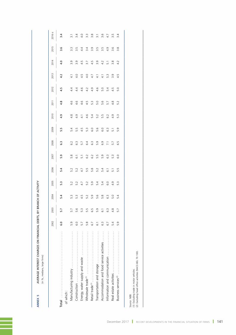
141December 2017 ❙ REcENt DEvElopmENtS IN tHE fINANcIAl SItuAtIoN of fIRmS ❙
An
nex
5
AV
ERA
GE
INTE
RES
T C
HA
RG
ES O
N F
INA
NC
IAL
DEB
TS,
BY
BR
AN
CH
OF
AC
TIV
ITY
(in %
, m
edia
ns,
larg
e fir
ms)
2002
2003
2004
2005
2006
2007
2008
2009
2010
2011
2012
2013
2014
2015
2016
e
Tota
l .
....
....
....
....
....
....
....
....
....
....
.6.
05.
75.
45.
35.
45.
96.
35.
54.
94.
84.
54.
24.
03.
63.
4
of w
hich
:
Man
ufac
turin
g in
dust
ry .
....
....
....
....
....
..5.
95.
75.
35.
25.
25.
86.
25.
44.
84.
64.
44.
13.
93.
33.
1
Con
stru
ctio
n .
....
....
....
....
....
....
....
...
6.0
5.6
5.3
5.2
5.2
6.1
6.3
5.5
4.9
4.6
4.4
4.0
3.9
3.5
3.4
Ener
gy,
wat
er s
uppl
y an
d w
aste
..
....
....
....
.5.
75.
34.
54.
74.
75.
15.
74.
54.
14.
64.
64.
54.
54.
44.
0
Who
lesa
le t
rade
(1)
....
....
....
....
....
....
...
5.8
5.5
5.2
5.2
5.5
6.2
6.4
5.3
4.6
4.5
4.2
4.0
3.7
3.4
3.3
Reta
il tr
ade
(1) .
....
....
....
....
....
....
....
...
6.7
6.5
5.9
5.9
5.8
6.2
6.3
6.0
5.4
5.3
4.9
4.7
4.5
3.9
3.8
Tran
spor
tatio
n an
d st
orag
e ..
....
....
....
....
..6.
15.
95.
65.
45.
25.
55.
95.
65.
25.
04.
64.
13.
93.
53.
1
Acc
omm
odat
ion
and
food
ser
vice
act
iviti
es .
....
.6.
36.
15.
85.
45.
45.
96.
96.
05.
55.
65.
04.
14.
23.
53.
6
Info
rmat
ion
and
com
mun
icat
ion
...
....
....
....
6.7
6.3
6.3
6.0
6.1
6.3
7.1
6.3
6.2
5.7
5.4
5.3
5.1
4.9
4.7
Real
est
ate
activ
ities
...
....
....
....
....
....
...
5.4
4.8
5.0
4.9
5.1
5.3
5.7
5.1
4.9
4.8
4.5
3.9
3.8
3.6
3.5
Busi
ness
ser
vice
s (2)
....
....
....
....
....
....
...
5.9
5.7
5.4
5.3
5.5
6.0
6.5
5.9
5.3
5.2
5.0
4.5
4.2
3.8
3.4
Sour
ce :
NBB
.(1
) Ex
clud
ing
trad
e in
mot
or v
ehic
les.
(2)
Excl
udin
g he
ad o
ffic
e ac
tiviti
es (
NA
CE-
BEL
70 1
00).

142 ❙ REcENt DEvElopmENtS IN tHE fINANcIAl SItuAtIoN of fIRmS ❙ NBB Economic Review
An
nex
6
TAN
GIB
LE F
IXED
ASS
ET R
ENEW
AL
RA
TE B
Y B
RA
NC
H O
F A
CTI
VIT
Y
(in %
, gl
obal
ised
dat
a)
2002
2003
2004
2005
2006
2007
2008
2009
2010
2011
2012
2013
2014
2015
2016
e
Tota
l .
....
....
....
....
....
....
....
....
....
....
.23
.222
.823
.325
.324
.126
.026
.121
.219
.321
.620
.219
.419
.819
.420
.2
of w
hich
:
Man
ufac
turin
g in
dust
ry .
....
....
....
....
....
..24
.624
.023
.423
.324
.427
.526
.421
.420
.021
.823
.521
.823
.424
.925
.0
Con
stru
ctio
n .
....
....
....
....
....
....
....
...
25.7
23.7
22.2
24.7
27.2
31.8
31.2
27.0
21.6
25.8
20.9
19.1
19.1
19.6
18.7
Ener
gy,
wat
er s
uppl
y an
d w
aste
..
....
....
....
.11
.210
.415
.716
.311
.413
.117
.925
.718
.315
.915
.016
.210
.711
.416
.7
Who
lesa
le t
rade
(1)
....
....
....
....
....
....
...
31.4
26.8
27.8
28.1
31.2
30.8
28.5
22.4
22.4
24.6
22.8
21.7
21.5
20.5
21.8
Reta
il tr
ade
(1) .
....
....
....
....
....
....
....
...
28.0
24.6
25.2
25.7
25.9
26.4
25.6
22.7
22.4
31.8
22.5
20.4
21.2
21.5
22.0
Tran
spor
tatio
n an
d st
orag
e ..
....
....
....
....
..26
.422
.726
.949
.923
.426
.926
.320
.519
.117
.214
.616
.322
.218
.819
.9
Acc
omm
odat
ion
and
food
ser
vice
act
iviti
es .
....
.15
.914
.216
.016
.017
.321
.121
.315
.316
.015
.215
.612
.913
.513
.715
.6
Info
rmat
ion
and
com
mun
icat
ion
...
....
....
....
21.8
20.0
22.0
26.3
26.8
25.6
32.8
21.3
18.8
24.8
24.7
27.5
27.5
24.4
23.9
Real
est
ate
activ
ities
...
....
....
....
....
....
...
10.5
12.8
12.3
12.3
12.5
12.9
15.5
11.9
10.9
11.7
11.7
11.3
12.5
10.9
11.5
Busi
ness
ser
vice
s (2)
....
....
....
....
....
....
...
29.1
30.1
31.9
30.5
30.6
32.0
31.7
26.0
26.4
33.4
29.8
26.1
25.5
26.0
27.6
Sour
ce :
NBB
.(1
) Ex
clud
ing
trad
e in
mot
or v
ehic
les.
(2)
Excl
udin
g he
ad o
ffic
e ac
tiviti
es (
NA
CE-
BEL
70 1
00).

December 2017 ❙ ABStRActS fRom tHE WoRkINg pApERS SERIES ❙ 143
Abstracts from the Working papers series
328. Firm heterogeneity and aggregate business services exports : Micro evidence from Belgium, France, Germany and Spain, by A. Ariu, E. Biewen, S. Blank, G. Guillaume, M.J. Gonzales, Ph. Meinen, D. Mirza, C. Martin, P. Tello, September 2017
The paper uses detailed micro data on service exports at the firm-destination-service level to analyse the role of firm heterogeneity in shaping aggregate service exports in Belgium, France, Germany and Spain from 2003 to 2007. The authors decompose the level and the growth of aggregate service exports into different trade margins paying special attention to firm heterogeneity within countries. They find that the weak export growth of France is at least partly due to poor performance by small exporters. By contrast, small exporters are the most dynamic contributors to the aggregate exports of Belgium, Germany and Spain. Their results highlight the importance of firm heterogeneity in understanding aggregate export growth.
329. The interconnections between services and goods trade at the firm-level, by A. Ariu, H. Breinlichz, G. Corcosx, G. Mion, October 2017
In the paper the authors study how international trade in goods and services interact at the firm level. Using a rich dataset on Belgian firms during the period 1995-2005, they show that : i) firms are much more likely to source services and goods inputs from the same origin country rather than from different ones ; ii) increases in barriers to imports of goods reduce firm-level imports of services from the same market, and conversely. They build upon a discrete-choice model of goods and services input sourcing that can reproduce these facts to design our econometric strategy. the results suggest that a liberalization of service trade has direct and sizable effects on goods trade and vice‑versa. moreover, sourcing goods and services from the same origin brings substantial complementarities to both.
330. Why do manufacturing firms produce services ? Evidence for the servitization paradox in Belgium, by P. Blanchard, C. Fuss, C. Mathieu, November 2017
The increasing role of services in GDP results from the growing share of service industries, but also from the fact that firms produce services along with goods. The paper investigates the determinants of service provision by manufacturing firms. First, it develops a model of differentiated products with, on the demand side, complementarities between the firm’s goods and services, and, on the supply side, rivalry in the allocation of expertise between the production of goods and the provision of services. Second, it provides an econometric assessment of the determinants of servitization for manufacturing firms, using a fractional Probit model with heterogeneity, controlling for endogeneity with respect to unobserved firm characteristics. Both the theoretical model and empirical estimates point to a non-linear relationship between servitization and firm productivity. The relationship is further shaped by the sector environment as well as intrinsic characteristics of the goods and services supplied.

December 2017 ❙ coNvENtIoNAl SIgNS ❙ 145
conventional signs
% per cente.g. exempli gratia (for example)etc. et ceterai.e. id est (that is)p.m. pro memoria

December 2017 ❙ lISt of ABBREvIAtIoNS ❙ 147
list of abbreviations
Countries or regions
Be BelgiumDe Germanyee estoniaIe IrelandeL Greecees spainFR FranceIt ItalyCY CyprusLt LithuaniaLV LatviaLU LuxembourgMt MaltanL netherlandsAt AustriaPt PortugalsI sloveniasK slovakiaFI Finland
eA euro area
BG BulgariaCZ Czech RepublicDK DenmarkHR CroatiaHU HungaryPL PolandRo Romaniase swedenUK United Kingdom
eU european UnioneU15 european Union, excluding countries that joined after 2003

148 ❙ lISt of ABBREvIAtIoNS ❙ NBB Economic Review
CH switzerlandIs IcelandJP Japanno norwayUs United states
other abbreviations
APP Asset purchase programme
BB Budgetary balance
CnC Commission des normes comptables (Accounting standards Board)CPB Central Planning Bureau (the netherlands)
DGs Directorate General statistics
eC european CommissioneCB european Central BankeDIs european Deposit Insurance schemeeFsF european Financial stability FacilityeFsM european Financial stabilisation MechanismeMU economic and Monetary Unioneonia euro overnight Index AverageesA european system of Accounts esCB european system of Central BanksesM european stability Mechanism
FDI Foreign direct investmentFPB Federal Planning BureauFPs Federal Public serviceFte Full-time equivalent
GDP Gross domestic product
HICP Harmonised index of consumer prices
IDR In-depth reviewIMF International Monetary Fund
MIP Macroeconomic imbalance procedureMto Medium-term objective
nACe nomenclature of economic activities in the european CommunitynACe-BeL nomenclature of economic activities in the european Community – Belgian
versionnAI national Accounts InstitutenBB national Bank of BelgiumnBeR national Bureau of economic ResearchnCPI national consumer price indexneo national employment officenPI non-profit institution

December 2017 ❙ lISt of ABBREvIAtIoNS ❙ 149
oeCD organisation for economic Cooperation and DevelopmentoG output gapoMt outright monetary transactionsoPeC organisation of the Petroleum exporting Countries
R&D Research and development
sB structural balancesGP stability and Growth Pacts&P standard and Poor’ssMe small and medium-sized enterprisesoWALFIn société Wallonne de Financement et de Garantie des Petites et Moyennes
entreprisessPF survey of Professional ForecasterssRIW société Régionale d’Investissement de WalloniesRM single resolution mechanismssM single supervisory mechanismsUst sustainable budgetary balance
tFeU treaty on the Functioning of the european UniontLtRo targeted longer-term refinancing operationstPF total factor productivitytsCG treaty on stability, Coordination and Governance
Un United nations
VAt Value added tax
ZLB Zero lower bound

E N T R E P R I S E
ECOONDERNEMING
DYNAMIQUEDYNAMISCHE
BRUXELLESENVIRONNEMENT
LEEFMILIEUBRUSSEL
label n. 2008/132/3
National Bank of Belgiumlimited liability companyRLP Brussels – Company number : 0203.201.340Registered office : boulevard de Berlaimont 14 – BE - 1000 Brusselswww.nbb.be
publisher
jan Smetsgovernor
National Bank of BelgiumBoulevard de Berlaimont 14 – BE ‑ 1000 Brussels
contact for the publication
pierre crevitsHead of general Secretariat and communication
Tel. +32 2 221 30 [email protected]
© Illustrations : National Bank of Belgium
Cover and layout : NBB AG – Prepress & Image
published in february 2018


