57
Economics 173 Business Statistics Lectures 15 - 18 Summer, 2001 Professor J. Petry
| Date post: | 13-Dec-2015 |
| Category: |
Documents |
| Upload: | bruno-cunningham |
| View: | 215 times |
| Download: | 1 times |
Economics 173Business Statistics
Lectures 15 - 18
Summer, 2001
Professor J. Petry

Simple Linear Regression Simple Linear Regression and Correlationand Correlation
Chapter 17

17.1 Introduction
• In this chapter we employ Regression Analysisto examine the relationship among quantitative variables.
• The technique is used to predict the value of one variable (the dependent variable - y)based on the value of other variables (independent variables x1, x2,…xk.)

17.2 The Model
• The first order linear model
y = dependent variablex = independent variable0 = y-intercept1 = slope of the line = error variable
xy 10 xy 10
x
y
0 Run
Rise = Rise/Run
0 and 1 are unknown,therefore, are estimated from the data.

17.3 Estimating the Coefficients
• The estimates are determined by – drawing a sample from the population of interest,– calculating sample statistics.– producing a straight line that cuts into the data.
The question is:Which straight line fits best?
x
y

3
3
The best line is the one that minimizes the sum of squared vertical differences between the points and the line.
41
1
4
(1,2)
2
2
(2,4)
(3,1.5)
Sum of squared differences = (2 - 1)2 + (4 - 2)2 + (1.5 - 3)2 +
(4,3.2)
(3.2 - 4)2 = 6.89Sum of squared differences = (2 -2.5)2 + (4 - 2.5)2 + (1.5 - 2.5)2 + (3.2 - 2.5)2 = 3.99
2.5
Let us compare two linesThe second line is horizontal
The smaller the sum of squared differencesthe better the fit of the line to the data.

To calculate the estimates of the coefficientsthat minimize the differences between the data points and the line, use the formulas:
xbyb
xnx
yxnyx
s
YXb
i
ii
x
10
2221
),cov(
xbyb
xnx
yxnyx
s
YXb
i
ii
x
10
2221
),cov(
The regression equation that estimatesthe equation of the first order linear modelis:
xbby 10 xbby 10
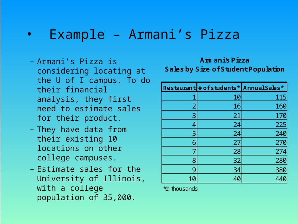
• Example – Armani’s Pizza
– Armani’s Pizza is considering locating at the U of I campus. To do their financial analysis, they first need to estimate sales for their product.
– They have data from their existing 10 locations on other college campuses.
– Estimate sales for the University of Illinois, with a college population of 35,000.
Armani's PizzaSales by Size of Student Population
Restaurant # of students* Annual Sales*
1 10 1152 16 1603 21 1704 24 2255 24 2406 27 2707 28 2748 32 2809 34 380
10 40 440
*in thousands
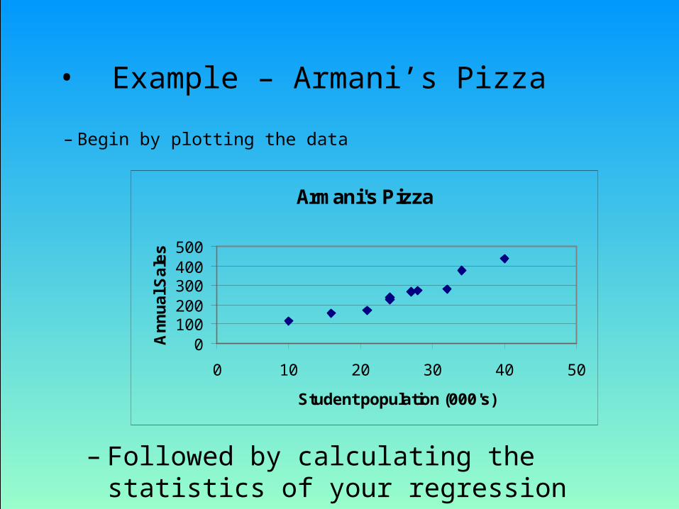
• Example – Armani’s Pizza
– Begin by plotting the data
Armani's Pizza
0100200300400500
0 10 20 30 40 50
Student population (000's)
An
nu
al S
ale
s
– Followed by calculating the statistics of your regression
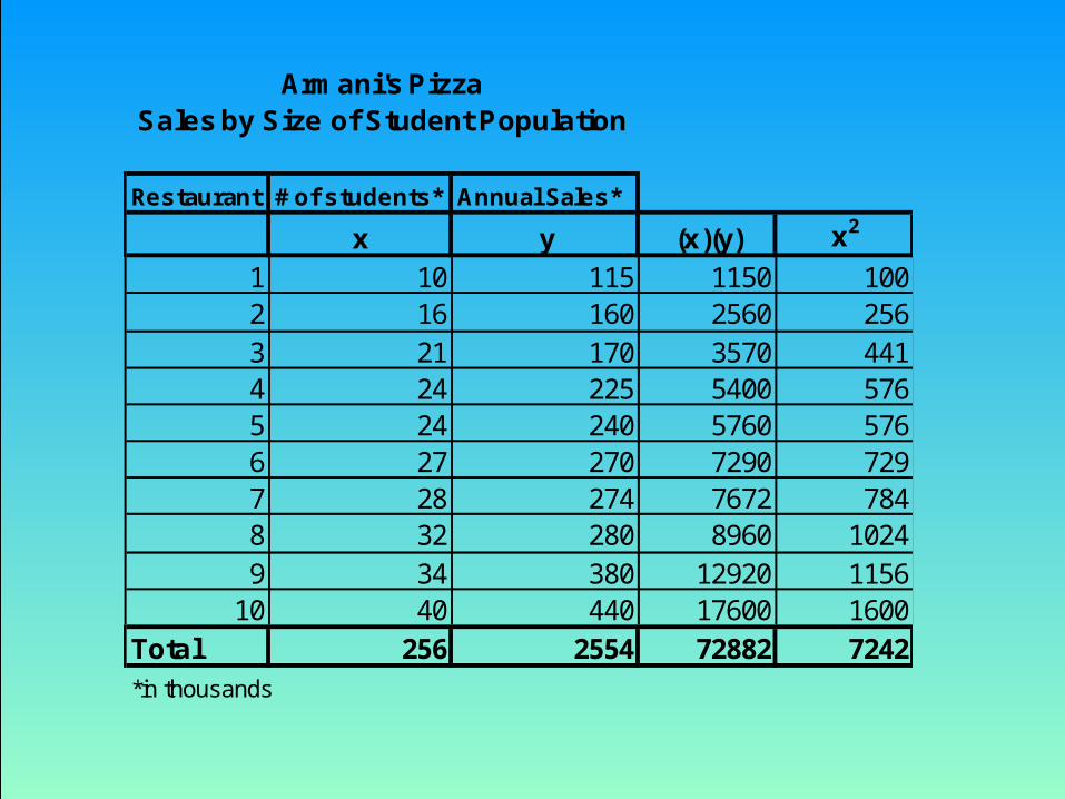
Armani's PizzaSales by Size of Student Population
Restaurant # of students* Annual Sales*
x y (x)(y) x2
1 10 115 1150 1002 16 160 2560 2563 21 170 3570 4414 24 225 5400 5765 24 240 5760 5766 27 270 7290 7297 28 274 7672 7848 32 280 8960 10249 34 380 12920 1156
10 40 440 17600 1600Total 256 2554 72882 7242
*in thousands
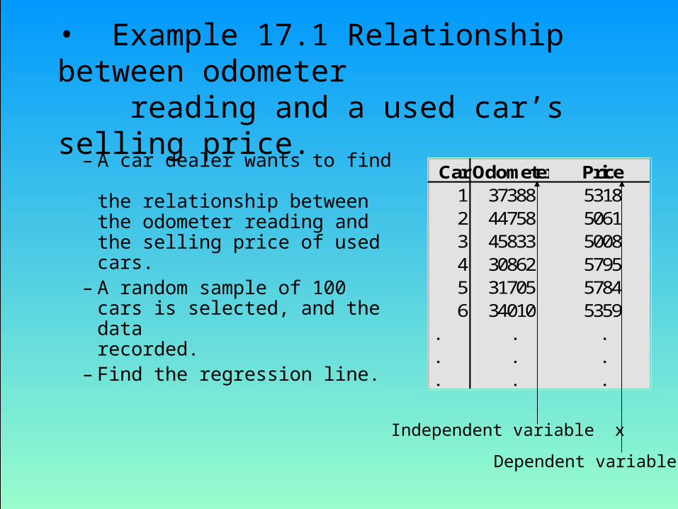
• Example 17.1 Relationship between odometer reading and a used car’s selling price.
– A car dealer wants to find the relationship between the odometer reading and the selling price of used cars.
– A random sample of 100 cars is selected, and the data recorded.
– Find the regression line.
Car Odometer Price1 37388 53182 44758 50613 45833 50084 30862 57955 31705 57846 34010 5359
. . .
. . .
. . .
Independent variable x
Dependent variable y

• Solution– Solving by hand
• To calculate b0 and b1 we need to calculate several statistics first;
;41.411,5y
;45.009,36x
256,356,11
))((),cov(
688,528,431
)( 22
n
yyxxYX
n
xxs
ii
ix
where n = 100.
533,6)45.009,36)(0312.(41.5411xbyb
0312.688,528,43256,356,1
s
)Y,Xcov(b
10
2x
1
x0312.533,6xbby 10
4500
5000
5500
6000
19000 29000 39000 49000
OdometerP
rice
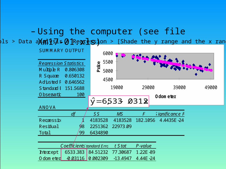
– Using the computer (see file Xm17-01.xls)
SUMMARY OUTPUT
Regression StatisticsMultiple R 0.806308R Square 0.650132Adjusted R Square0.646562Standard Error151.5688Observations 100
ANOVAdf SS MS F Significance F
Regression 1 4183528 4183528 182.1056 4.4435E-24Residual 98 2251362 22973.09Total 99 6434890
CoefficientsStandard Error t Stat P-valueIntercept 6533.383 84.51232 77.30687 1.22E-89Odometer -0.03116 0.002309 -13.4947 4.44E-24
x0312.533,6y
Tools > Data analysis > Regression > [Shade the y range and the x range] > OK
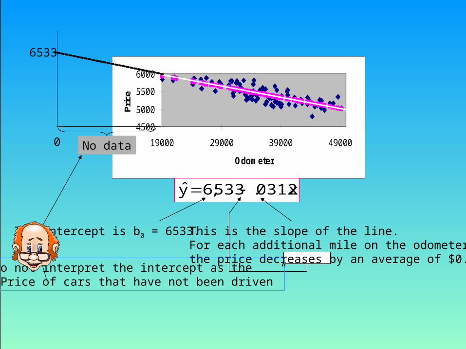
This is the slope of the line.For each additional mile on the odometer,the price decreases by an average of $0.0312
4500
5000
5500
6000
19000 29000 39000 49000
Odometer
Pric
e
x0312.533,6y
The intercept is b0 = 6533.
6533
0 No data
Do not interpret the intercept as the “Price of cars that have not been driven”

17.4 Error Variable: Required Conditions
• The error is a critical part of the regression model.• Four requirements involving the distribution of must
be satisfied.– The probability distribution of is normal.– The mean of is zero: E() = 0.– The standard deviation of is for all values of x.– The set of errors associated with different values of y are
all independent.
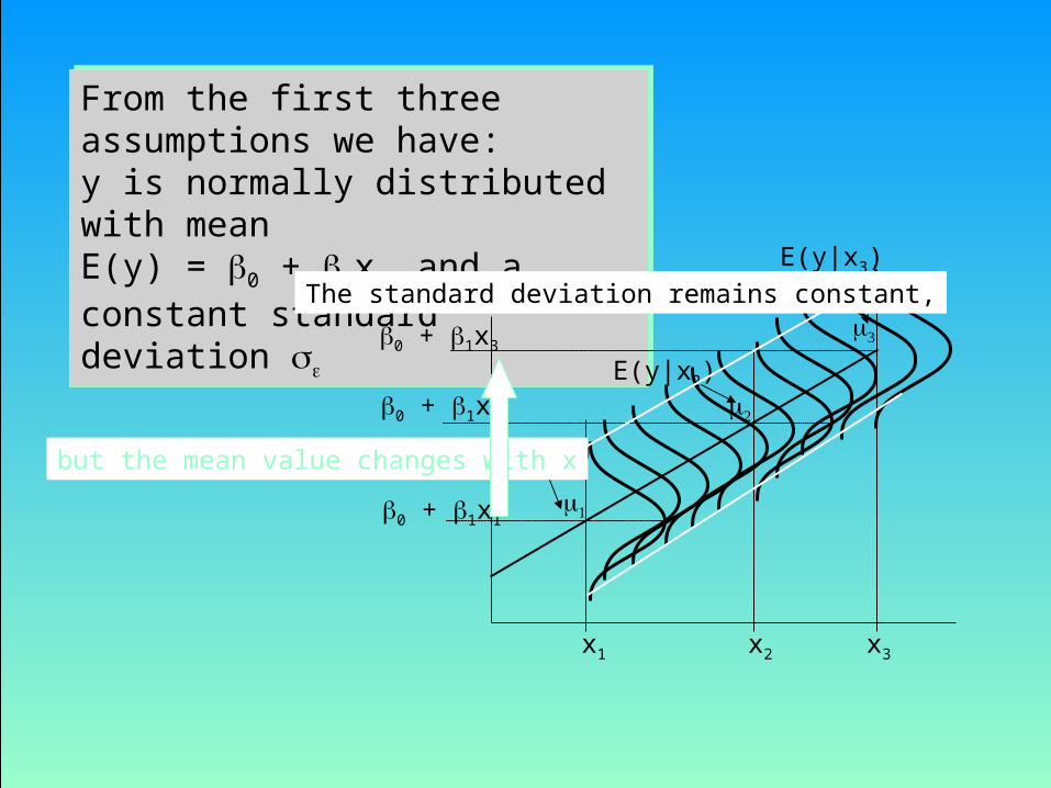
From the first three assumptions we have:y is normally distributed with meanE(y) = 0 + 1x, and a constant standard deviation
From the first three assumptions we have:y is normally distributed with meanE(y) = 0 + 1x, and a constant standard deviation
0 + 1x1
0 + 1x2
0 + 1x3
E(y|x2)
E(y|x3)
x1 x2 x3
E(y|x1)
The standard deviation remains constant,
but the mean value changes with x

17.5 Assessing the Model
• The least squares method will produce a regression line whether or not there is a linear relationship between x and y.
• Consequently, it is important to assess how well the linear model fits the data.
• Several methods are used to assess the model:– Testing and/or estimating the coefficients.– Using descriptive measurements.
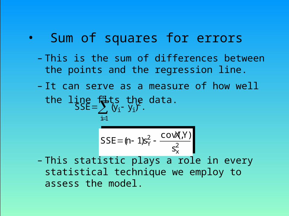
– This is the sum of differences between the points and the regression line.
– It can serve as a measure of how well the line fits the data.
– This statistic plays a role in every statistical technique we employ to assess the model.
2x
2Y
s
)Y,Xcov(s)1n(SSE
2x
2Y
s
)Y,Xcov(s)1n(SSE
.)yy(SSEn
1i
2ii
• Sum of squares for errors
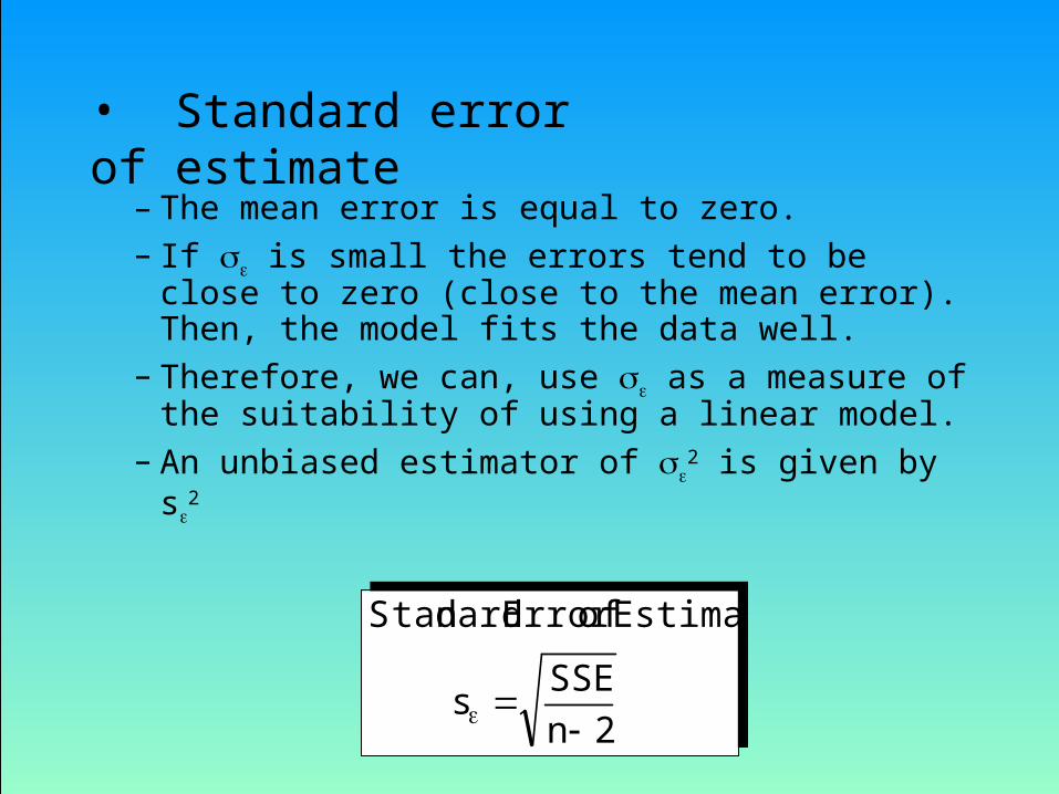
– The mean error is equal to zero.– If is small the errors tend to be close to zero
(close to the mean error). Then, the model fits the data well.
– Therefore, we can, use as a measure of the suitability of using a linear model.
– An unbiased estimator of 2 is given by s
2
2nSSE
s
EstimateofErrordardtanS
2nSSE
s
EstimateofErrordardtanS
• Standard error of estimate

• Example 17.2– Calculate the standard error of estimate for example
17.1, and describe what does it tell you about the model fit?
• Solution
6.15198
363,251,2
2
,
363,252,2688,528,43
)256,356,1()999,64(99
),cov()1(
999,6499
890,434,6
1
)ˆ(
2
22
22
n
SSEs
Thus
s
YXsnSSE
n
yys
xY
iiY
Calculated before
It is hard to assess the model based on s even when compared with the mean value of y.
4.411,5y,6.151s
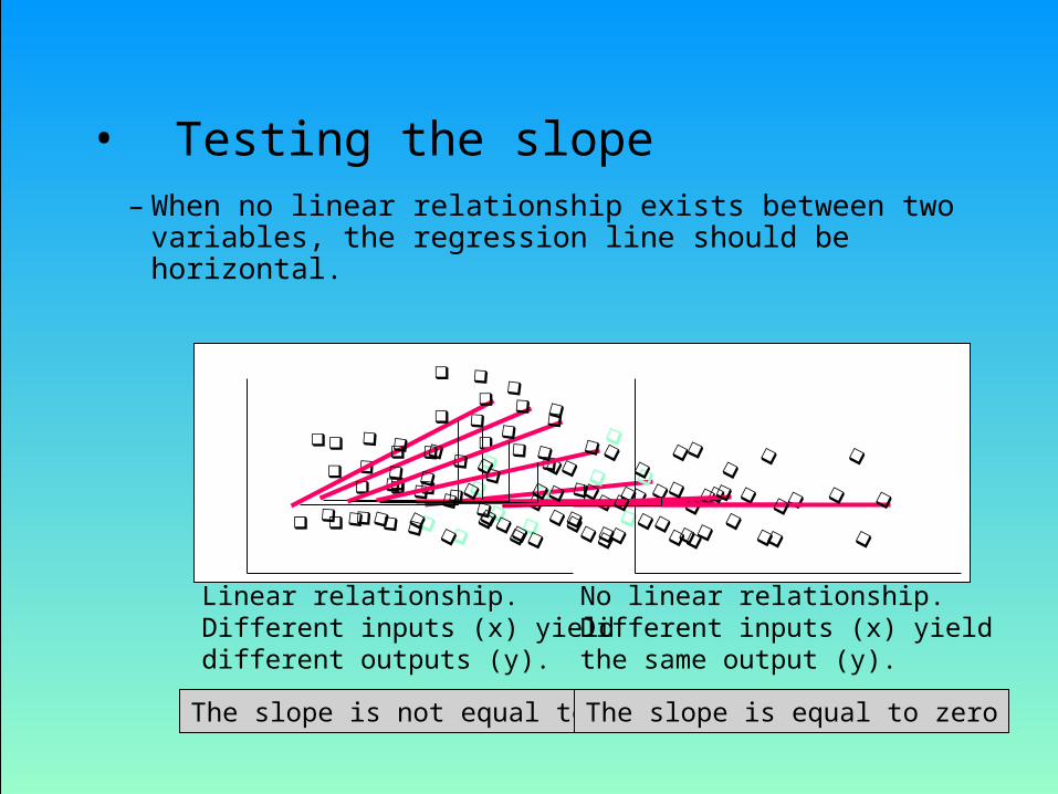
• Testing the slope– When no linear relationship exists between two
variables, the regression line should be horizontal.
Linear relationship.Different inputs (x) yielddifferent outputs (y).
No linear relationship.Different inputs (x) yieldthe same output (y).
The slope is not equal to zero The slope is equal to zero

• We can draw inference about 1 from b1 by testingH0: 1 = 0
H1: 1 = 0 (or < 0,or > 0)– The test statistic is
– If the error variable is normally distributed, the statistic is Student t distribution with d.f. = n-2.
1b
11
sb
t
1b
11
sb
t
The standard error of b1.
2x
bs)1n(
ss
1
2x
bs)1n(
ss
1
where

• Solution– Solving by hand– To compute “t” we need the values of b1 and sb1.
49.1300231
0312
00231.688,528,43)(99(
6.151
)1(
312.
1
1
11
2
1
..
s
bt
sn
ss
b
b
x
b
– Using the computerCoefficients Standard Error t Stat P-value
Intercept 6533.383035 84.51232199 77.30687 1.22E-89Odometer -0.031157739 0.002308896 -13.4947 4.44E-24
There is overwhelming evidence to inferthat the odometer reading affects the auction selling price.

• Example– Evaluate the model used in the Armani’s Pizza example by
testing the value of the slope. You are given:
0722.1)1(
89425.10
2
1
1
x
bsn
ss
b

• Coefficient of determination
– When we want to measure the strength of the linear relationship, we use the coefficient of determination.
SST
SSR
SST
SSERor
ss
YXR
yx
1)],[cov( 2
22
22
SST
SSR
SST
SSERor
ss
YXR
yx
1)],[cov( 2
22
22

– To understand the significance of this coefficient note:
Overall variability in y
The regression model
Remains, in part, unexplained The error
Explained in part by

x1 x2
y1
y2
y
Two data points (x1,y1) and (x2,y2) of a certain sample are shown.
22
21 )yy()yy( 2
22
1 )yy()yy( 222
211 )yy()yy(
Total variation in y = Variation explained by the regression line)
+ Unexplained variation (error)

• R2 measures the proportion of the variation in y that is explained by the variation in x.
SST
SSR
SST
SSESST
SST
SSER
12
Variation in y (SST) = SSR + SSE
• R2 takes on any value between zero and one.R2 = 1: Perfect match between the line and the data points.R2 = 0: There are no linear relationship between x and y.
Regression StatisticsMultiple R 0.8063R Square 0.6501
Adjusted R Square 0.6466Standard Error 151.57Observations 100
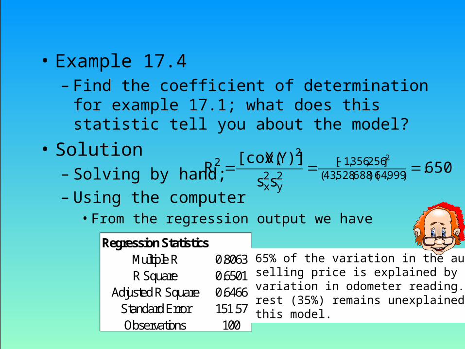
• Example 17.4– Find the coefficient of determination for example 17.1;
what does this statistic tell you about the model?• Solution
– Solving by hand;– Using the computer
• From the regression output we have
6501.ss
)]Y,X[cov(R )999,64)(688,528,43(
]256,356,1[2y
2x
22 2
65% of the variation in the auctionselling price is explained by the variation in odometer reading. Therest (35%) remains unexplained bythis model.

• Example– Find the coefficient of determination for the Armani’s
Pizza example; what does this statistic tell you about the model? You are given values of SSR = 81702.499, and SSE = 6331.901. Regression Statistics
Multiple R 0.963366334R Square 0.928074693Adjusted R Square 0.91908403Standard Error 28.13339035
SUMMARY OUTPUT Observations 10
ANOVAdf SS MS F Significance F
Regression 1 81702.49878 81702.49878 103.2264983 7.5384E-06Residual 8 6331.90122 791.4876525Total 9 88034.4
Coefficients Standard Error t Stat P-value Lower 95% Upper 95%Intercept -23.49273678 28.85565265 -0.814146783 0.439120548 -90.0340341 43.04856X Variable 1 10.89424753 1.072263792 10.16004421 7.53839E-06 8.42160119 13.36689
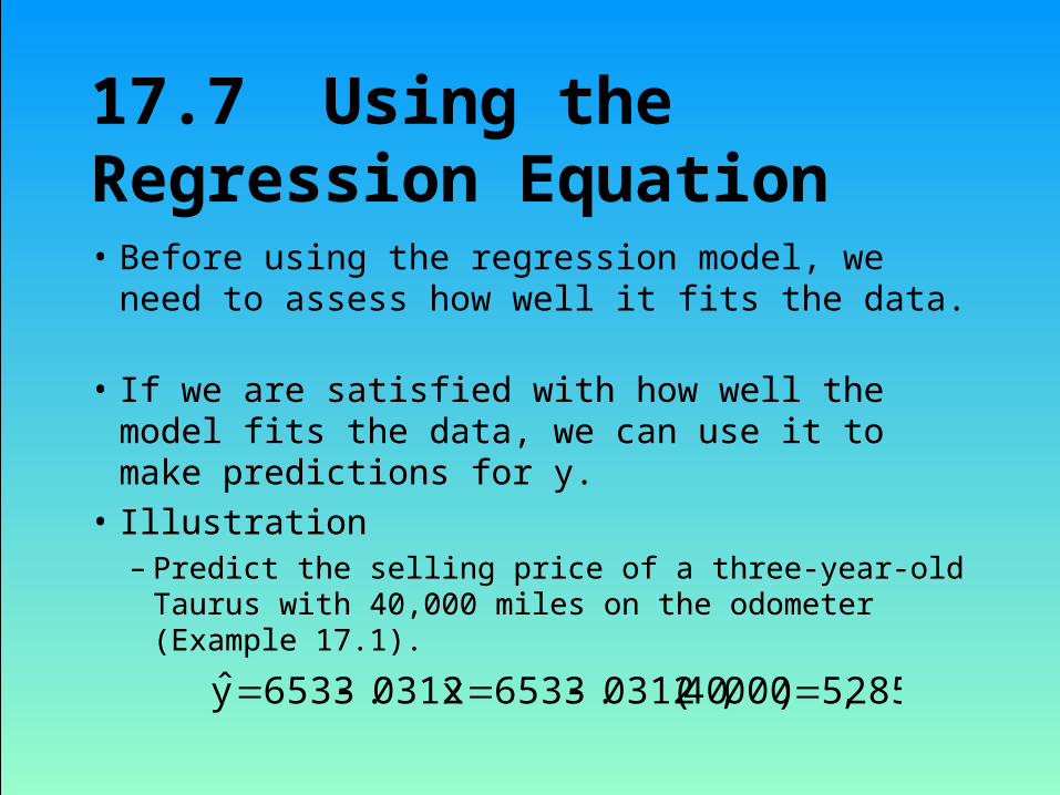
17.7 Using the Regression Equation
• If we are satisfied with how well the model fits the data, we can use it to make predictions for y.
• Illustration– Predict the selling price of a three-year-old Taurus
with 40,000 miles on the odometer (Example 17.1).285,5)000,40(0312.6533x0312.6533y
• Before using the regression model, we need to assess how well it fits the data.
• If we are satisfied with how well the model fits the data, we can use it to make predictions for y.
• Illustration– Predict the selling price of a three-year-old Taurus
with 40,000 miles on the odometer (Example 17.1).

• Prediction interval and confidence interval
– Two intervals can be used to discover how closely the predicted value will match the true value of y.
• Prediction interval - for a particular value of y,• Confidence interval - for the expected value of y.
– The confidence interval– The confidence interval
2
i
2g
2)xx(
)xx(
n1
sty
2
i
2g
2)xx(
)xx(
n1
sty
– The prediction interval– The prediction interval
2
i
2g
2)xx(
)xx(
n1
1sty
2
i
2g
2)xx(
)xx(
n1
1sty
The prediction interval is wider than the confidence interval

• Example 17.6 interval estimates for the car auction price
– Provide an interval estimate for the bidding price on a Ford Taurus with 40,000 miles on the odometer.
– Solution• The dealer would like to predict the price of a single car
• The prediction interval(95%) =
2
i
2g
2)xx(
)xx(
n1
1sty
303285,5160,340,309,4
)009,36000,40(
100
11)6.151(984.1)]40000(0312.6533[
2
t.025,98

– The car dealer wants to bid on a lot of 250 Ford Tauruses, where each car has been driven for about 40,000 miles.
– Solution• The dealer needs to estimate the mean price per car.
• The confidence interval (95%) =
2
2
2 )(
)(1ˆ
xx
xx
nsty
i
g
35285,5160,340,309,4
)009,36000,40(100
1)6.151(984.1)]40000(0312.6533[
2
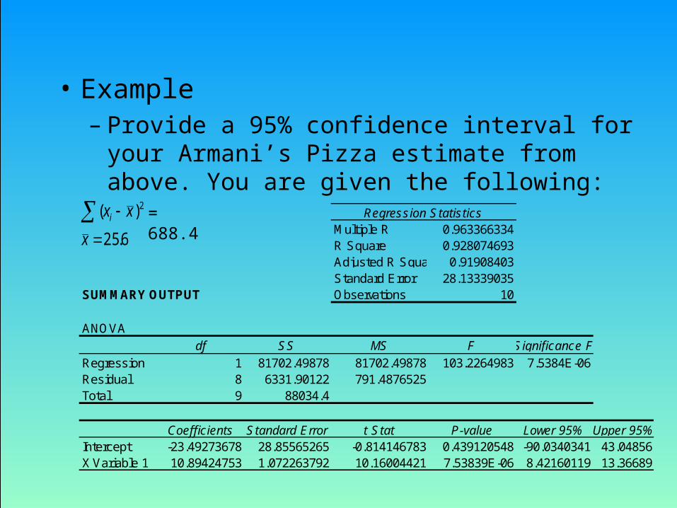
• Example– Provide a 95% confidence interval for your Armani’s
Pizza estimate from above. You are given the following:
Regression StatisticsMultiple R 0.963366334R Square 0.928074693Adjusted R Square 0.91908403Standard Error 28.13339035
SUMMARY OUTPUT Observations 10
ANOVAdf SS MS F Significance F
Regression 1 81702.49878 81702.49878 103.2264983 7.5384E-06Residual 8 6331.90122 791.4876525Total 9 88034.4
Coefficients Standard Error t Stat P-value Lower 95% Upper 95%Intercept -23.49273678 28.85565265 -0.814146783 0.439120548 -90.0340341 43.04856X Variable 1 10.89424753 1.072263792 10.16004421 7.53839E-06 8.42160119 13.36689
6.25
)( 2
x
xxi = 688.4

17.8 Coefficient of correlation
• The coefficient of correlation is used to measure the strength of association between two variables.
• The coefficient values range between -1 and 1.– If r = -1 (negative association) or r = +1 (positive
association) every point falls on the regression line.– If r = 0 there is no linear pattern.
• The coefficient can be used to test for linear relationship between two variables.

• Testing the coefficient of correlation– When there are no linear relationship between two
variables, = 0.– The hypotheses are:
H0: = 0H1: = 0
– The test statistic is:
yx
2
ss)Y,Xcov(
rbycalculated
ncorrelatiooftcoefficiensampletheisrwherer1
2nrt
The statistic is Student t distributedwith d.f. = n - 2, provided the variables are bivariate normally distributed.
X
Y

• Example 17.7 Testing for linear relationship
– Test the coefficient of correlation to determine if linear relationship exists in the data of example 17.1.
• Solution– We test H0: = 0
H1: 0.– Solving by hand:
• The rejection region is|t| > t/2,n-2 = t.025,98 = 1.984 or so.
• The sample coefficient of correlation r=cov(X,Y)/sxsy=-.806
The value of the t statistic is
Conclusion: There is sufficientevidence at = 5% to infer thatthere are linear relationshipbetween the two variables.
49.13r1
2nrt
2

• Example– Test at the 5% significance level whether a linear
relationship exists between student population and pizza sales at the University of Illinois.
– How do these results compare to your test of b1?

Project I: Finance Application• Project simulates the job of professional portfolio managers.• Your job is to advise high net-worth clients on investment decisions. This often involves “educating” the client.• Client is Medical Doctor, with little financial expertise, but serious cash ($1,000,000). • The stock market has declined significantly over the last year or so, and she believes now is the time to get in.• She gives you five stocks and asks which one she should invest in. How do you respond?

Project I: Finance ApplicationThe project is divided into three parts
1. Calculate mean, standard deviation and beta for each asset.– gather 5 years of historical monthly returns for your team’s five companies, the S&P 500 total return index and the 3-month constant maturity Treasury bill. Put in table and explain to client.
2. Illustrate benefits of diversification with concrete example. – You are provided with average annual returns and standard deviations for the S&P 500 and the 3-month T-bill. You create a portfolio with these two instruments weighted differently to illustrate the impact on risk (standard deviation).
3. Analyze impact of correlations on diversification.– Create table of correlation coefficients between all assets, and explain. Select asset pair with r closest to –1. Explain. – Adjust graph in 2 with r = 1, and –1 instead of 0. Explain.
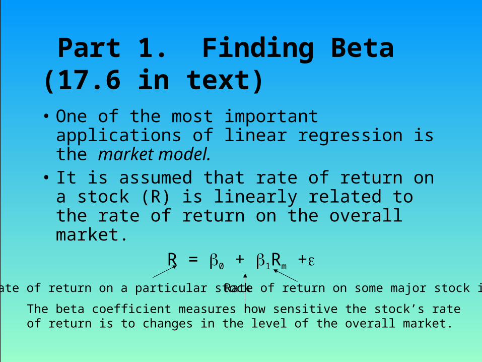
Part 1. Finding Beta (17.6 in text)
• One of the most important applications of linear regression is the market model.
• It is assumed that rate of return on a stock (R) is linearly related to the rate of return on the overall market.
R = 0 + 1Rm +
Rate of return on a particular stock Rate of return on some major stock index
The beta coefficient measures how sensitive the stock’s rate of return is to changes in the level of the overall market.
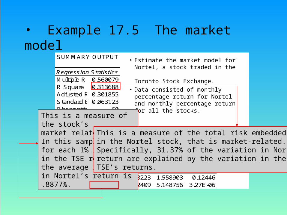
• Example 17.5 The market modelSUMMARY OUTPUT
Regression StatisticsMultiple R 0.560079R Square 0.313688Adjusted R Square0.301855Standard Error0.063123Observations 60
ANOVAdf SS MS F Significance F
Regression 1 0.10563 0.10563 26.50969 3.27E-06Residual 58 0.231105 0.003985Total 59 0.336734
CoefficientsStandard Error t Stat P-valueIntercept 0.012818 0.008223 1.558903 0.12446TSE 0.887691 0.172409 5.148756 3.27E-06
• Estimate the market model for Nortel, a stock traded in the Toronto Stock Exchange.
• Data consisted of monthly percentage return for Nortel and monthly percentage returnfor all the stocks.
This is a measure of the stock’smarket related risk. In this sample, for each 1% increase in the TSE return, the average increase in Nortel’s return is .8877%.
This is a measure of the total risk embeddedin the Nortel stock, that is market-related.Specifically, 31.37% of the variation in Nortel’sreturn are explained by the variation in the TSE’s returns.

Part 2. Diversification (Ex 6.8, sect 6.7)Investment portfolio diversification– An investor has decided to invest equal amounts of money
in two investments.
– Find the expected return on the portfolio– If = 1, .5, 0 find the standard deviation of the portfolio.
Mean returnStandard dev.Investment 1 15% 25%Investment 2 27% 40%
Mean returnStandard dev.Investment 1 15% 25%Investment 2 27% 40%
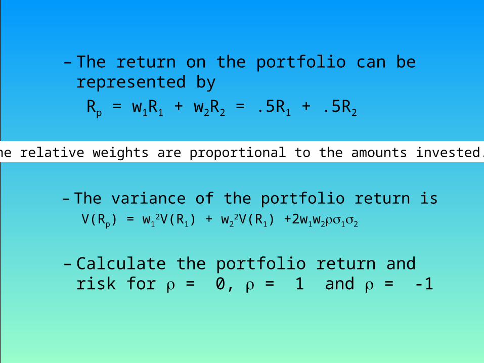
– The return on the portfolio can be represented by Rp = w1R1 + w2R2 = .5R1 + .5R2
The relative weights are proportional to the amounts invested.
– The variance of the portfolio return isV(Rp) = w1
2V(R1) + w22V(R1) +2w1w212
– Calculate the portfolio return and risk for = 0, = 1 and = -1
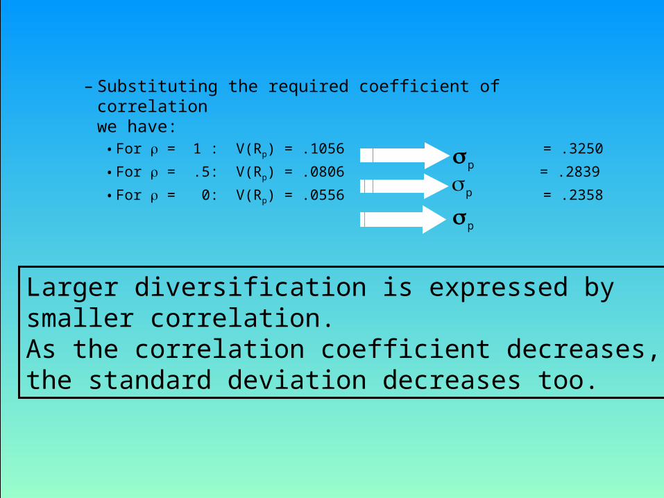
– Substituting the required coefficient of correlationwe have:
• For = 1 : V(Rp) = .1056 = .3250
• For = .5: V(Rp) = .0806 = .2839
• For = 0: V(Rp) = .0556 = .2358
Larger diversification is expressed bysmaller correlation.As the correlation coefficient decreases,the standard deviation decreases too.
pp
p

Benefits of DiversificationInvestment Proportion Portfolio
Bonds Stocks Expected Return Standard Deviation0% 100% 17.0% 25.0%
20% 80% 15.6% 20.1%40% 60% 14.2% 15.7%60% 40% 12.8% 12.3%80% 20% 11.4% 10.8%
100% 0% 10.0% 12.0%
Investment Opportunity Set
0.0%
2.0%
4.0%
6.0%
8.0%
10.0%
12.0%
14.0%
16.0%
18.0%
0.0% 5.0% 10.0% 15.0% 20.0% 25.0% 30.0%
Risk
Re
turn

17.9 Regression Diagnostics - I
• The three conditions required for the validity of the regression analysis are:– the error variable is normally distributed.– the error variance is constant for all values of x.– The errors are independent of each other.
• How can we diagnose violations of these conditions?

• Residual Analysis
– Examining the residuals (or standardized residuals), we can identify violations of the required conditions
– Example 17.1 - continued• Nonnormality.
– Use Excel to obtain the standardized residual histogram.– Examine the histogram and look for a bell shaped diagram with
mean close to zero.
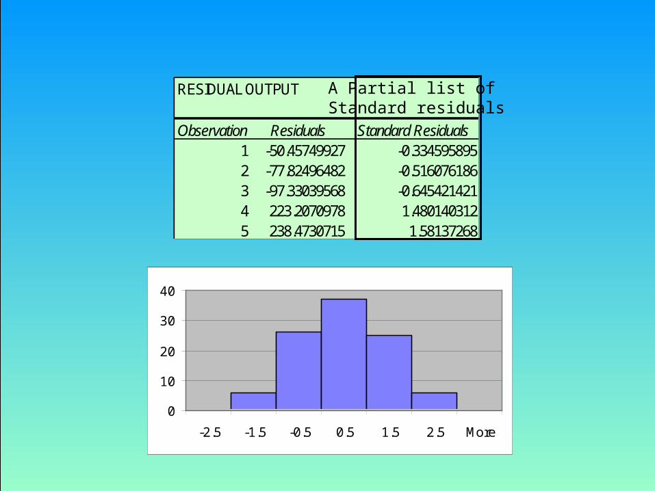
RESIDUAL OUTPUT
Observation Residuals Standard Residuals1 -50.45749927 -0.3345958952 -77.82496482 -0.5160761863 -97.33039568 -0.6454214214 223.2070978 1.4801403125 238.4730715 1.58137268
0
10
20
30
40
-2.5 -1.5 -0.5 0.5 1.5 2.5 More
A Partial list ofStandard residuals

• Heteroscedasticity
– When the requirement of a constant variance is violated we have heteroscedasticity.
+ + ++
+ ++
++
+
+
+
+
+
+
+
+
+
+
++
+
+
+
The spread increases with y
y
Residualy
+
+++
+
++
+
++
+
+++
+
+
+
+
+
++
+
+
+
+
+
+
++
+
++
+
+
+
+
+
+
+
+
+
+
++
+
+
+
y
Residualy
+
++
+
+++
+
+
+
+
+
++
+
++
+
+
+
++
+
++
+
++
++
+
+
+
+
++
+
++
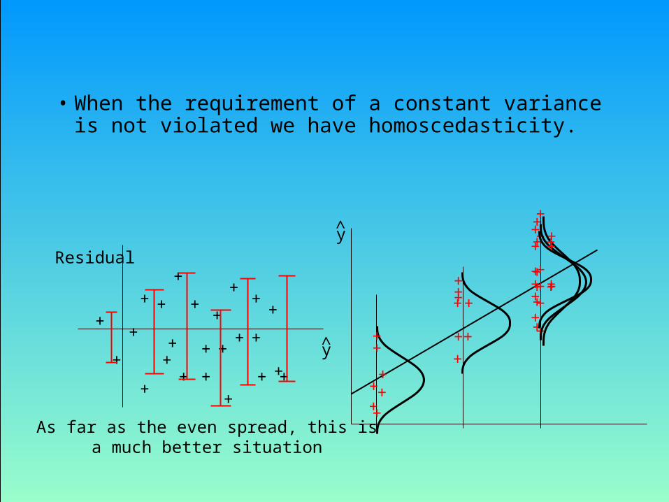
As far as the even spread, this isa much better situation
• When the requirement of a constant variance is not violated we have homoscedasticity.
• Nonindependence of error variables
– A time series is constituted if data were collected over time.
– Examining the residuals over time, no pattern should be observed if the errors are independent.
– When a pattern is detected, the errors are said to be autocorrelated.
– Autocorrelation can be detected by graphing the residuals against time.

+
+++ +
++
++
+ +
++ + +
+
++ +
+
+
+
+
+
+Time
Residual Residual
Time+
+
+
Patterns in the appearance of the residuals over time indicates that autocorrelation exists.
Note the runs of positive residuals,replaced by runs of negative residuals
Note the oscillating behavior of the residuals around zero.
0 0

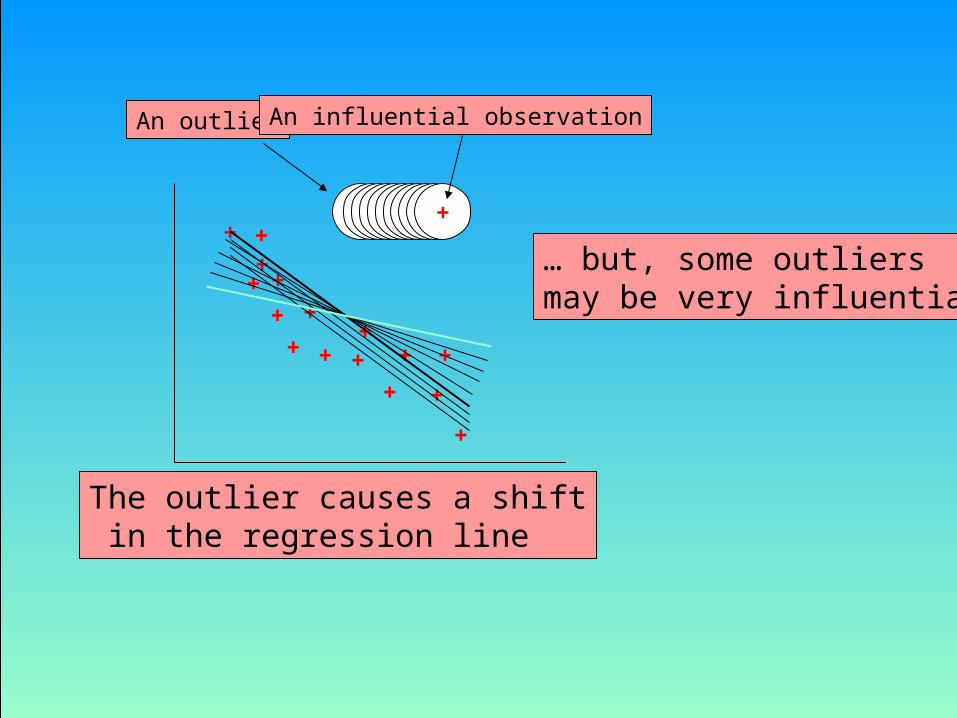
• Outliers
– An outlier is an observation that is unusually small or large.
– Several possibilities need to be investigated when an outlier is observed:
• There was an error in recording the value.• The point does not belong in the sample.• The observation is valid.
– Identify outliers from the scatter diagram.– It is customary to suspect an observation is an outlier if
its |standard residual| > 2
+
+
+
+
+ +
+ + ++
+
+
+
+
+
+
+
The outlier causes a shift in the regression line
… but, some outliers may be very influential
++++++++++
An outlier An influential observation
• Procedure for regression diagnostics
– Develop a model that has a theoretical basis.– Gather data for the two variables in the model.– Draw the scatter diagram to determine whether a
linear model appears to be appropriate.– Check the required conditions for the errors.– Assess the model fit.– If the model fits the data, use the regression
equation.


