28
Economics 20 - Prof. An derson 1 Multiple Regression Analysis y = 0 + 1 x 1 + 2 x 2 + . . . k x k + u 1. Estimation
| Date post: | 14-Dec-2015 |
| Category: |
Documents |
| Upload: | ean-goodger |
| View: | 219 times |
| Download: | 0 times |

Economics 20 - Prof. Anderson 1
Multiple Regression Analysis
y = 0 + 1x1 + 2x2 + . . . kxk + u
1. Estimation
Economics 20 - Prof. Anderson 2
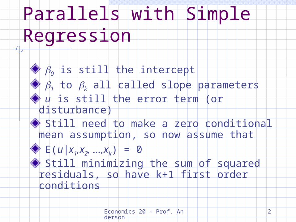
Parallels with Simple Regression
0 is still the intercept
1 to k all called slope parameters u is still the error term (or disturbance) Still need to make a zero conditional mean assumption, so now assume that
E(u|x1,x2, …,xk) = 0 Still minimizing the sum of squared residuals, so have k+1 first order conditions

Economics 20 - Prof. Anderson 3
Interpreting Multiple Regression
tioninterpreta a
has each is that ,ˆˆ
thatimplies fixed ,..., holding so
,ˆ...ˆˆˆ
so ,ˆ...ˆˆˆˆ
11
2
2211
22110
ribus ceteris pa
xy
xx
xxxy
xxxy
k
kk
kk
Economics 20 - Prof. Anderson 4
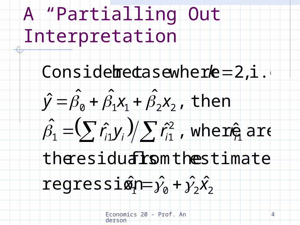
A “Partialling Out” Interpretation
2201
12111
22110
ˆˆˆˆ regression
estimated thefrom residuals the
are ˆ where,ˆˆˆ
then ,ˆˆˆˆ
i.e. ,2 wherecase heConsider t
xx
rryr
xxy
k
iiii

Economics 20 - Prof. Anderson 5
“Partialling Out” continued
Previous equation implies that regressing y on x1 and x2 gives same effect of x1 as regressing y on residuals from a regression of x1 on x2
This means only the part of xi1 that is uncorrelated with xi2 is being related to yi so we’re estimating the effect of x1 on y after x2 has been “partialled out”
Economics 20 - Prof. Anderson 6
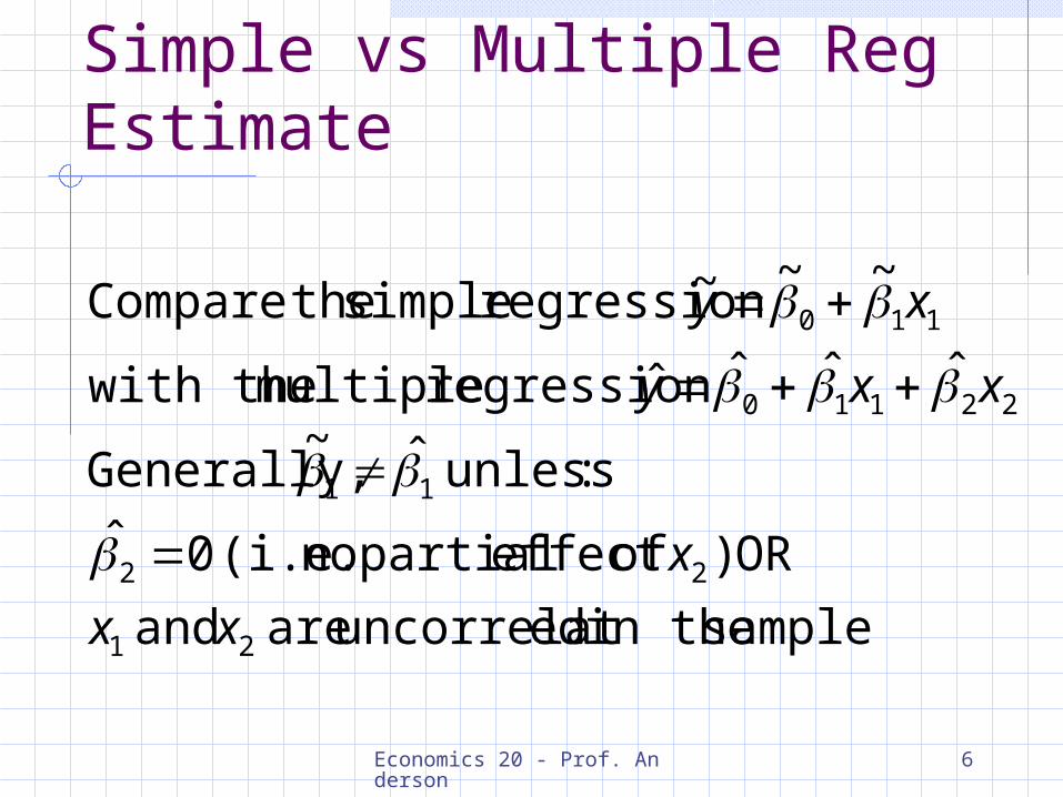
Simple vs Multiple Reg Estimate
sample in the eduncorrelat are and
OR ) ofeffect partial no (i.e. 0ˆ
:unless ˆ~ Generally,
ˆˆˆˆ regression multiple with the
~~~ regression simple theCompare
21
22
11
22110
110
xx
x
xxy
xy

Economics 20 - Prof. Anderson 7
Goodness-of-Fit
SSR SSE SSTThen
(SSR) squares of sum residual theis ˆ
(SSE) squares of sum explained theis ˆ
(SST) squares of sum total theis
:following thedefine then Weˆˆ
part, dunexplainean and part, explainedan of up
made being asn observatioeach ofcan think We
2
2
2
i
i
i
iii
u
yy
yy
uyy
Economics 20 - Prof. Anderson 8
Goodness-of-Fit (continued)
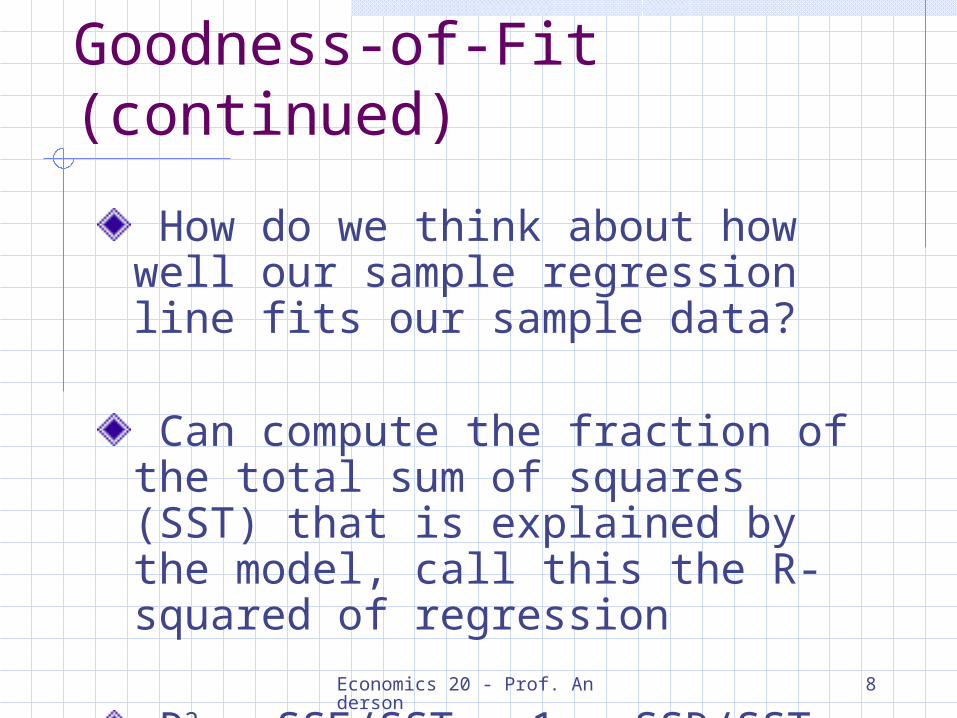
How do we think about how well our sample regression line fits our sample data?
Can compute the fraction of the total sum of squares (SST) that is explained by the model, call this the R-squared of regression
R2 = SSE/SST = 1 – SSR/SST

Economics 20 - Prof. Anderson 9
Goodness-of-Fit (continued)
22
2
2
2
ˆˆ
ˆˆ
ˆ values theand actual the
betweent coefficienn correlatio squared the
toequal being as of think alsocan We
yyyy
yyyyR
yy
R
ii
ii
ii
Economics 20 - Prof. Anderson 10
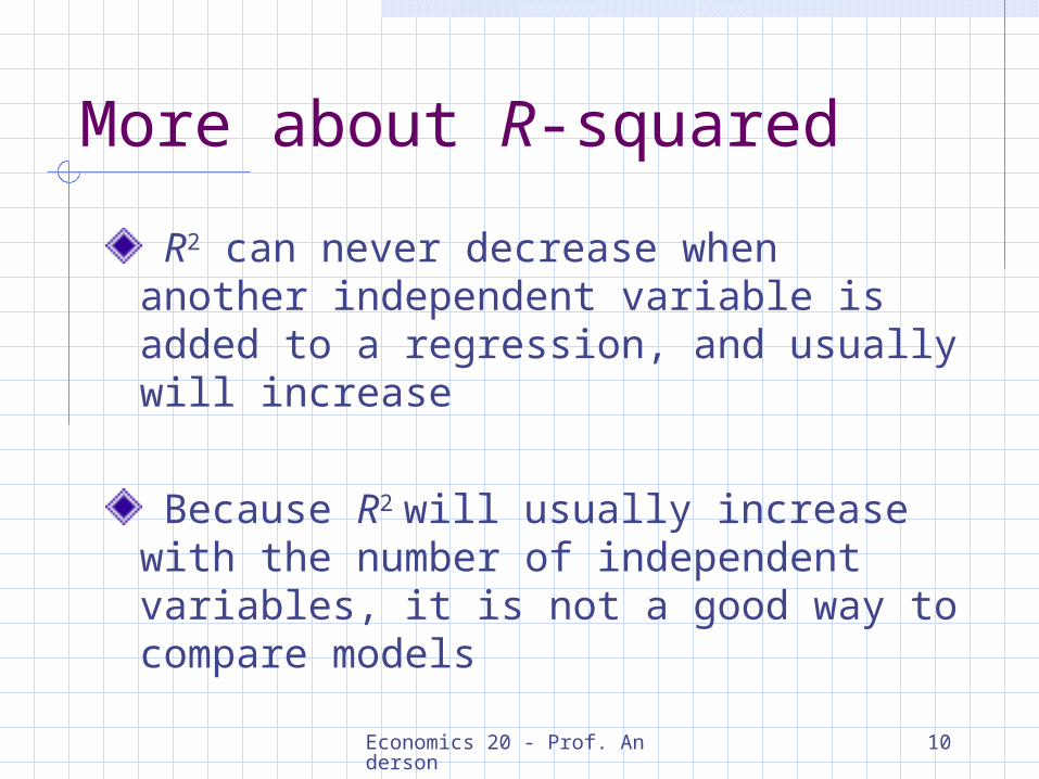
More about R-squared
R2 can never decrease when another independent variable is added to a regression, and usually will increase
Because R2 will usually increase with the number of independent variables, it is not a good way to compare models
Economics 20 - Prof. Anderson 11
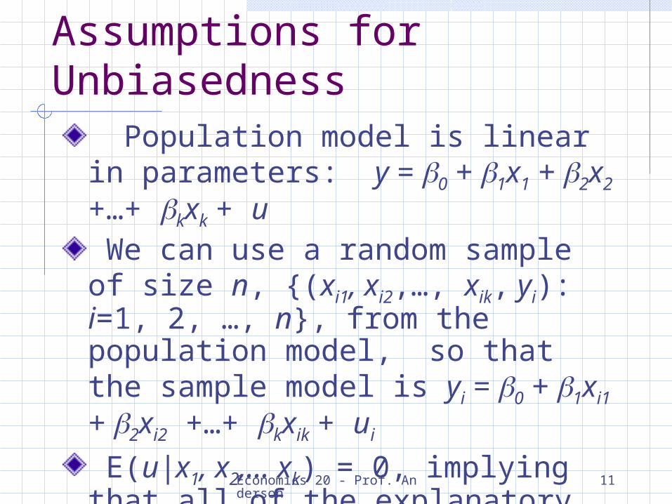
Assumptions for Unbiasedness Population model is linear in parameters: y = 0 + 1x1 + 2x2 +…+ kxk + u We can use a random sample of size n, {(xi1, xi2,…, xik, yi): i=1, 2, …, n}, from the population model, so that the sample model is yi = 0 + 1xi1 + 2xi2 +…+ kxik + ui
E(u|x1, x2,… xk) = 0, implying that all of the explanatory variables are exogenous None of the x’s is constant, and there are no exact linear relationships among them

Economics 20 - Prof. Anderson 12
Too Many or Too Few Variables
What happens if we include variables in our specification that don’t belong? There is no effect on our parameter estimate, and OLS remains unbiased
What if we exclude a variable from our specification that does belong? OLS will usually be biased
Economics 20 - Prof. Anderson 13
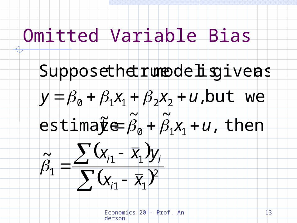
Omitted Variable Bias
211
111
110
22110
~
then,~~~ estimate
but we ,
asgiven is model true theSuppose
xx
yxx
uxy
uxxy
i
ii
Economics 20 - Prof. Anderson 14
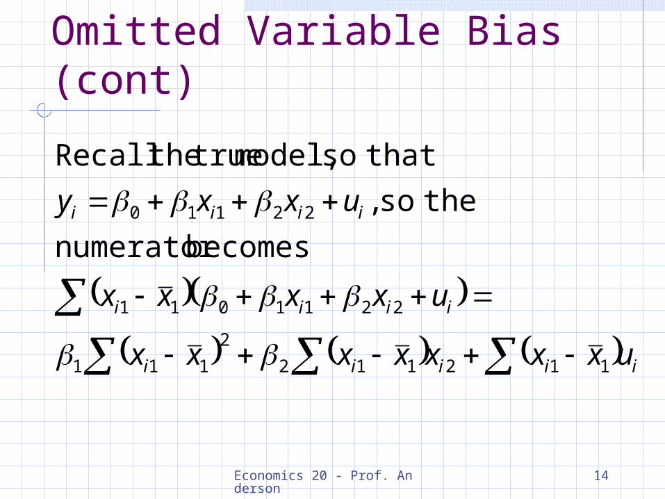
Omitted Variable Bias (cont)
iiiii
iiii
iiii
uxxxxxxx
uxxxx
uxxy
112112
2
111
2211011
22110
becomesnumerator
theso ,
thatso model, true theRecall

Economics 20 - Prof. Anderson 15
Omitted Variable Bias (cont)
211
211211
211
11
211
21121
~
have wensexpectatio taking0,)E( since
~
xx
xxxE
u
xx
uxx
xx
xxx
i
ii
i
i
ii
i
ii
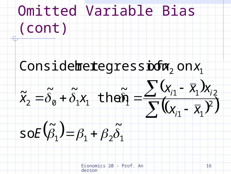
Economics 20 - Prof. Anderson 16
Omitted Variable Bias (cont)
1211
211
21111102
12
~~ so
~ then
~~~
on of regression heConsider t
E
xx
xxxxx
xx
i
ii

Economics 20 - Prof. Anderson 17
Summary of Direction of Bias
Corr(x1, x2) > 0 Corr(x1, x2) < 0
2 > 0 Positive bias Negative bias
2 < 0 Negative bias Positive bias
Economics 20 - Prof. Anderson 18
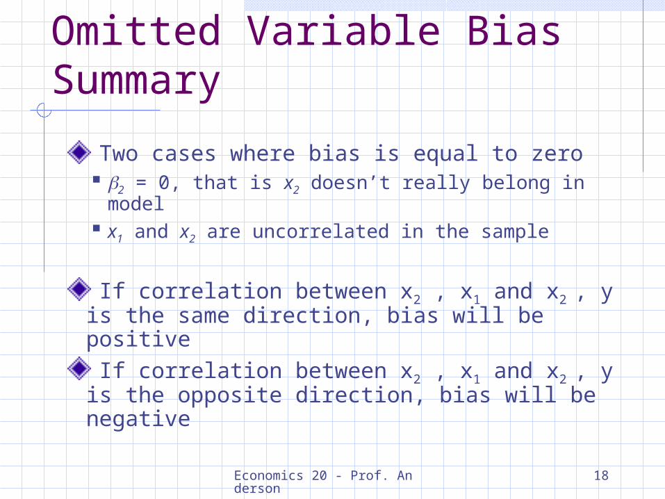
Omitted Variable Bias Summary
Two cases where bias is equal to zero 2 = 0, that is x2 doesn’t really belong in model x1 and x2 are uncorrelated in the sample
If correlation between x2 , x1 and x2 , y is the same direction, bias will be positive
If correlation between x2 , x1 and x2 , y is the opposite direction, bias will be negative
Economics 20 - Prof. Anderson 19
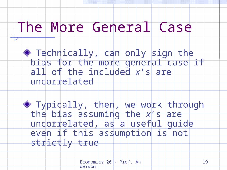
The More General Case
Technically, can only sign the bias for the more general case if all of the included x’s are uncorrelated
Typically, then, we work through the bias assuming the x’s are uncorrelated, as a useful guide even if this assumption is not strictly true

Economics 20 - Prof. Anderson 20
Variance of the OLS Estimators
Now we know that the sampling distribution of our estimate is centered around the true parameter Want to think about how spread out this distribution is Much easier to think about this variance under an additional assumption, so
Assume Var(u|x1, x2,…, xk) = 2 (Homoskedasticity)
Economics 20 - Prof. Anderson 21
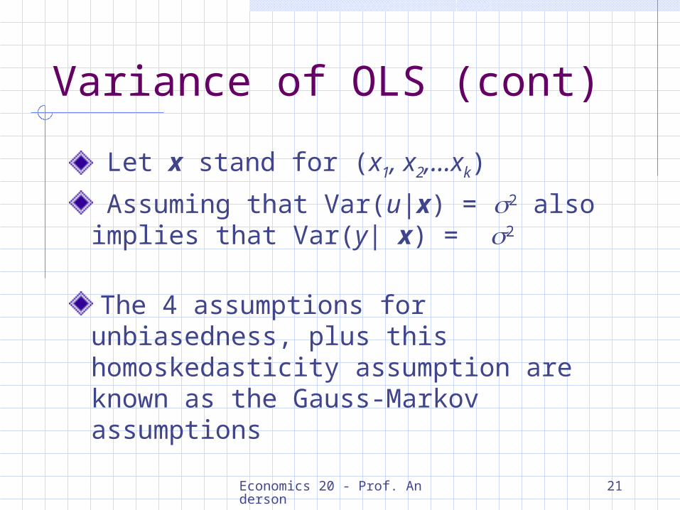
Variance of OLS (cont)
Let x stand for (x1, x2,…xk)
Assuming that Var(u|x) = 2 also implies that Var(y| x) = 2
The 4 assumptions for unbiasedness, plus this homoskedasticity assumption are known as the Gauss-Markov assumptions
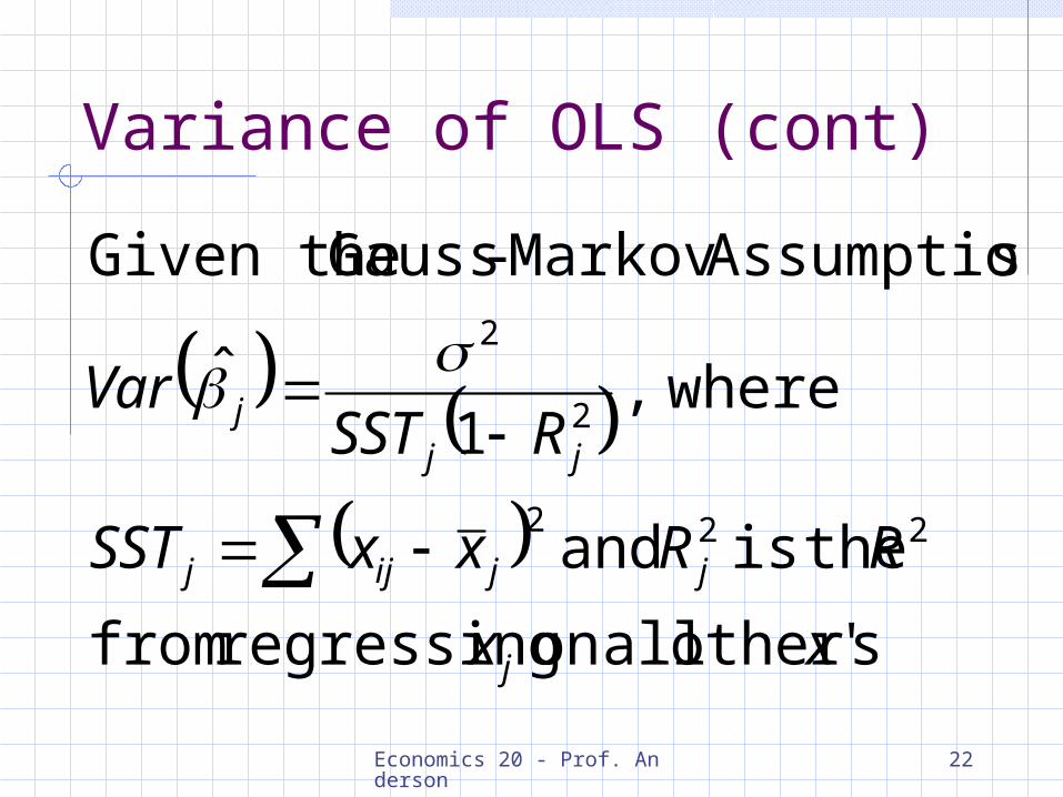
Economics 20 - Prof. Anderson 22
Variance of OLS (cont)
s'other allon regressing from
theis and
where,1
ˆ
sAssumption Markov-Gauss Given the
222
2
2
xx
RRxxSST
RSSTVar
j
jjijj
jjj
Economics 20 - Prof. Anderson 23
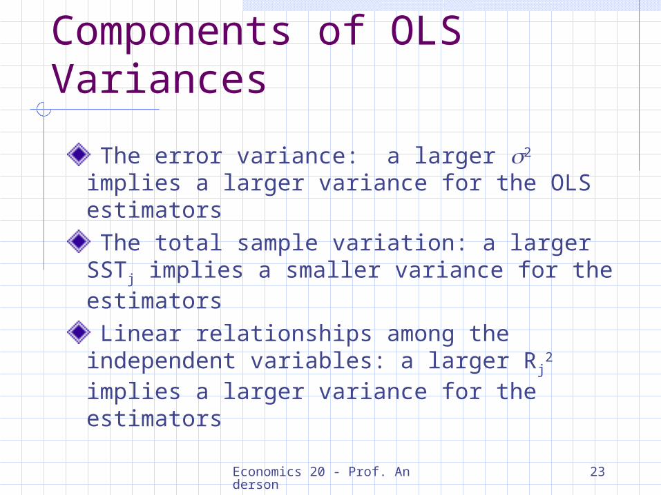
Components of OLS Variances
The error variance: a larger 2 implies a larger variance for the OLS estimators
The total sample variation: a larger SSTj implies a smaller variance for the estimators
Linear relationships among the independent variables: a larger Rj
2 implies a larger variance for the estimators
Economics 20 - Prof. Anderson 24
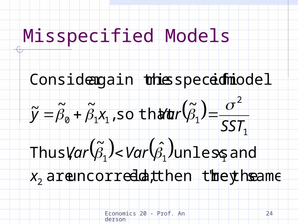
Misspecified Models
same there' then theyed,uncorrelat are
and unless ˆ~ Thus,
~ that so ,
~~~
model edmisspecifi again theConsider
2
111
1
2
1110
x
xVarVar
SSTVarxy

Economics 20 - Prof. Anderson 25
Misspecified Models (cont)
While the variance of the estimator is smaller for the misspecified model, unless 2 = 0 the misspecified model is biased
As the sample size grows, the variance of each estimator shrinks to zero, making the variance difference less important
Economics 20 - Prof. Anderson 26
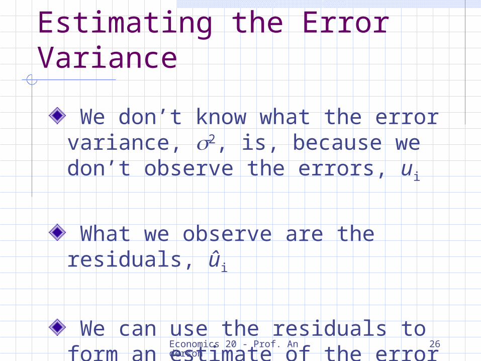
Estimating the Error Variance
We don’t know what the error variance, 2, is, because we don’t observe the errors, ui
What we observe are the residuals, ûi
We can use the residuals to form an estimate of the error variance

Economics 20 - Prof. Anderson 27
Error Variance Estimate (cont)
212
22
1ˆˆ thus,
1ˆˆ
jjj
i
RSSTse
dfSSRknu
df = n – (k + 1), or df = n – k – 1 df (i.e. degrees of freedom) is the (number of observations) – (number of estimated parameters)
Economics 20 - Prof. Anderson 28
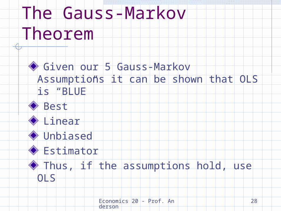
The Gauss-Markov Theorem
Given our 5 Gauss-Markov Assumptions it can be shown that OLS is “BLUE”
Best
Linear
Unbiased
Estimator
Thus, if the assumptions hold, use OLS


![ROOM ESSENCE No.417 Light Furniture K K-134NV K K ......ROOM ESSENCE No.417 Light Furniture K K-134NV K K-1340R ¥ 12,500 (Ëéfl]) WOO x cm X 120 x 80 KK-140GY 185818 KK-140NV 186211](https://static.documents.pub/doc/80x56/60ff5ab6e7dbf06e7d5abd9d/room-essence-no417-light-furniture-k-k-134nv-k-k-room-essence-no417-light.jpg)

![k|x/L lgodfjnL, @)&! · -6_ æk|x/L cltl/Qm cfo'QmÆ eGgfn] dxfgu/Lo k|x/L cGtu{t sfo{/t k|x/L gfoj dxflg/LIfs ;Demg' k5{ . -7_ æk|x/L cfo'QmÆ eGgfn] dxfgu/Lo k|x/L sfof{nosf] k|d'v](https://static.documents.pub/doc/80x56/6077828ea38c8056df0a6097/kxl-lgodfjnl-6-kxl-cltlqm-cfoqm-eggfn-dxfgulo-kxl-cgtut.jpg)


